Cache Telepathy: Leveraging Shared Resource Attacks to Learn DNN Architectures

Abstract

Deep Neural Networks (DNNs) are fast becoming ubiquitous for their ability to attain good accuracy in various machine learning tasks. A DNN’s architecture (i.e., its hyper-parameters) broadly determines the DNN’s accuracy and performance, and is often confidential. Attacking a DNN in the cloud to obtain its architecture can potentially provide major commercial value. Further, attaining a DNN’s architecture facilitates other, existing DNN attacks.

This paper presents Cache Telepathy: a fast and accurate mechanism to steal a DNN’s architecture using the cache side channel. Our attack is based on the insight that DNN inference relies heavily on tiled GEMM (Generalized Matrix Multiply), and that DNN architecture parameters determine the number of GEMM calls and the dimensions of the matrices used in the GEMM functions. Such information can be leaked through the cache side channel.

This paper uses Prime+Probe and Flush+Reload to attack VGG and ResNet DNNs running OpenBLAS and Intel MKL libraries. Our attack is effective in helping obtain the architectures by very substantially reducing the search space of target DNN architectures. For example, for VGG using OpenBLAS, it reduces the search space from more than $10^{35}$ architectures to just 16.

1 Introduction

For the past several years, Deep Neural Networks (DNNs) have increased in popularity thanks to their ability to attain high accuracy and performance in a multitude of machine learning tasks — e.g., image and speech recognition [1, 2], scene generation [3], and game playing [4]. An emerging framework that provides end-to-end infrastructure for using DNNs is Machine Learning as a Service (MLaaS) [5, 6]. In MLaaS, trusted clients submit DNNs or training data to MLaaS service providers (e.g., an Amazon or Google datacenter). Service providers host the DNNs, and allow remote untrusted users to submit queries to the DNNs for a fee.

Despite its promise, MLaaS provides new ways to undermine the privacy of the hosted DNNs. An adversary may be able to learn details of the hosted DNNs beyond the official query API. For example, an adversary may try to learn the DNN’s architecture (i.e., its hyper-parameters). These are the parameters that give the network its shape, such as the number and types of layers, the number of neurons per layer, and the connections between layers.

The architecture of a DNN broadly determines the DNN’s accuracy and performance. For this reason, obtaining it often has high commercial value. In addition, it generally takes a large amount of time and resources to try to obtain it by tuning hyper-parameters through training. Further, once a DNN’s architecture is known, other attacks are possible, such as the model extraction attack [7] (which obtains the weights of the DNN’s edges), and the membership inference attack [8],[9] (which determines whether a input was used to train the DNN).

Yet, stealing a DNN’s architecture is challenging. First, DNNs have a multitude of hyper-parameters, which makes brute-force guesswork unfeasible. Further, the DNN design space has been growing with time, which is further aggravating the adversary’s task.

This paper proves that despite the large search space, attackers can quickly and accurately recover DNN architectures in the MLaaS setting using the cache size channel. Our insight is that DNN inference relies heavily on tiled GEMM (Generalized Matrix Multiply), and that DNN architecture parameters determine the number of GEMM calls and the dimensions of the matrices used in the GEMM functions. Such information can be leaked through the cache side channel.

We present an attack that we call Cache Telepathy. It is the first cache side channel attack on modern DNNs. It targets DNN inference on general-purpose processors, which are widely used for inference in existing MLaaS platforms, such as Facebook’s [10] and Amazon’s [11].

We demonstrate our attack by implementing it on a state-of-the-art platform. We use Prime+Probe and Flush+Reload to attack the VGG and ResNet DNNs running OpenBLAS and Intel MKL libraries. Our attack is effective at helping obtain the architectures by very substantially reducing the search space of target DNN architectures. For example, for VGG using OpenBLAS, it reduces the search space from more than $10^{35}$ architectures to just 16.

This paper makes the following contributions:

1. It provides a detailed analysis of the mapping of DNN hyper-parameters to the number of GEMM calls and their arguments.

2. It implements the first cache-based side channel attack to extract DNN architectures on general purpose processors.

3. It evaluates the attack on VGG and ResNet DNNs running OpenBLAS and Intel MKL libraries.

2 Background

2.1 Deep Neural Networks

Deep Neural Networks (DNNs) are a class of ML algorithms that use a cascade of multiple layers of nonlinear processing units for feature extraction and transformation [12]. There are several major types of DNNs in use today, two popular types being fully-connected neural networks (or multi-layer perceptrons) and convolutional neural networks (CNNs).

DNN Architecture

The architecture of a DNN, also called the hyper-parameters, gives the network its shape. DNN hyper-parameters considered in this paper are:

1. Total number of layers.

2. Layer types, such as fully-connected, convolutional, or pooling layer.

3. Connections between layers, including sequential and non-sequential connections such as shortcuts and branches. Non-sequential connections exist in recent DNNs, such as ResNet [2]. For example, a shortcut consists of summing up the output of two different layers and using the result as input for a later layer.

4. Hyper-parameters for each layer. For a fully-connected layer, this is the number of neurons in that layer. For a convolutional layer, this is the number of filters, the filter size, and the striding size.

5. The activation function in each layer, e.g., relu and sigmoid.

DNN Weights

The DNN weights, also called parameters, specify operands to multiply-accumulates (MACCs) in the nested function. In a fully-connected layer, each edge out of a neuron is a MACC with a weight; in a convolutional layer, each filter is a sliding window that computes dot products over input neurons.

DNN Usage

DNNs usage is two distinct phases: training and inference. In training, the DNN designer starts with a network architecture and a training set of labeled inputs, and tries to find the DNN weights to minimize mis-prediction error. Training is generally performed offline on GPUs and takes a relatively long time to finish, typically hours or days [10],[13]. In inference, the trained model is deployed and used to make real-time predictions on new inputs. For good responsiveness, inference is generally performed on CPUs [10],[11]. Hyper-parameter tuning [14],[15] is the process of searching for the ideal DNN architecture. It requires training multiple DNNs with different architectures on the same data set. The DNN architecture search space may be large, meaning overall training takes significantly longer than the time to train a single DNN architecture.

2.2 Prior Privacy Attacks Need Architecture

To gain insight into the importance of DNN architectures, we discuss prior DNN privacy attacks [7, 8, 9, 16]. There are three types of such attacks, each with a different goal. All of them require knowing the victim’s DNN architecture. In the following, we refer to the victim’s network as the oracle network, its architecture as the oracle DNN architecture, and its training data set as the oracle training data set. In the model extraction attack [7], the attacker tries to obtain the weights of the oracle network. Although this attack is referred to as a “black-box” attack, it assumes that the attacker knows the oracle DNN architecture at the start. The attacker creates a synthetic data set, requests the classification results from the oracle network, and uses such results to train a network that uses the oracle architecture. The membership inference attack [8],[9] aims to infer the composition of the oracle training data set. This attack also requires knowledge of the oracle DNN architecture. The attacker creates multiple synthetic data sets and trains multiple networks that use the oracle architecture. Then, he runs the inference algorithm on these networks with some inputs in their training sets and some not in their training sets. He then compares the results and learns the output patterns of data in the training sets. He then uses this information to analyze the outputs of the oracle network running the inference algorithm on some inputs, and identifies those inputs that were in the oracle training data set. The hyper-parameter stealing attack [16] steals the loss function and regularization term used in ML algorithms, including DNN training and inference. This attack also relies on knowing the oracle DNN architecture. During the attack, the attacker leverages the model extraction attack to learn the DNN’s weights. He then finds the loss function that minimizes the training misprediction error.

2.3 Cache-based Side Channel Attacks

Flush+Reload [17] and Prime+Probe [18] are two powerful cache-base side channel attacks. They can extract secret keys [19, 20] and leak kernel and process information [21, 22].

Flush+Reload requires that the attacker share secure-sensitive code or data with the victim. This sharing can be achieved by leveraging the page de-duplication technique. It has been shown that de-duplication is widely deployed in public clouds to reduce the memory footprint and improve responsiveness [23]. In an attack, the attacker first performs a $\mathsf{clflush}$ operation to the shared cache line, to push it out of the cache. It then waits to allow the victim to execute. Finally, it re-accesses the same cache line and measures the access latency. Depending on the latency, it learns whether the victim has accessed the shared line.

Prime+Probe does not require page sharing. The attacker constructs a collection of addresses, called conflict addresses, which map to the same cache set as the victim’s line. In an attack, the attacker first accesses the conflict addresses to cause cache conflicts with the victim’s line, and evict it from the cache. After waiting for an interval, it re-accesses the conflict addresses and measures the access latency. The latency is used to infer whether the victim has accessed the line.

2.4 Threat Model

This paper develops a cache-timing attack that accurately reveals a DNN’s architecture. The attack relies on the following standard assumptions.

Co-location

We assume the attacker process can use techniques from prior work [24, 25] to co-locate onto the same processor chip as the victim process running DNN inference. This is feasible, as current MLaaS jobs are deployed on shared clouds. Note that recent MLaaS, such as Amazon SageMaker [26] and Google ML Engine [27] allow users to upload their own code for training and inference, instead of using pre-defined APIs. In this case, attackers can disguise themselves as an MLaaS process and the cloud scheduler will be unable to separate attacker processes from victim processes.

Code Analysis

We also assume that the attacker can analyze the ML framework code and linear algebra libraries used by the victim. These are realistic assumptions. First, open-source ML frameworks are widely used for efficient development of ML applications. The frameworks supported by Google, Amazon and other companies, including Tensorflow [28], Caffe [29], and MXNet [30] are all public. Our analysis is applicable to almost all of these frameworks. Second, the frameworks’ backends are all supported by high-performance and popular linear algebra libraries, such as OpenBLAS [31], Eigen [32] and MKL [33]. OpenBLAS and Eigen are open sourced, and MKL can be reverse engineered, as we show later. While we do not specifically address other algorithms such as FFT or Winograd, they are all amenable to cache-based attacks similar to those presented here.

3 Attack Overview

In this section, we discuss the challenge of reverse-engineering DNN architectures and our overall attack procedure.

Challenge of Reverse-Engineering DNN Architectures

A DNN’s architecture can be extracted in a search process, as shown in Figure 1. Specifically, the attacker constructs a synthetic dataset (①), and queries the oracle network for labels or confidence values (②), which are used as training data and labels. Then the attacker chooses a DNN architecture from a search space (③) to train a network (④). Steps ③-④ repeat until an architecture is found with sufficient prediction accuracy (⑤).

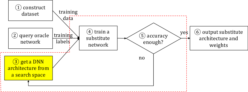
Figure 1: Searching DNN architectures.

This search process is extremely compute intensive, since it involves many iterations of step ④. Considering the depth and complexity of state-of-the-art DNNs, training and validating each network can take hours to days. Moreover, without any information about the architecture, the search space of possible architectures is often intractable. Thus, reverse engineering a DNN architecture by naively searching DNN architectures is unfeasible. The goal of Cache Telepathy is to reduce the architecture search space to a tractable size.

Overall Cache Telepathy Attack Procedure

We observe that DNN inference relies on GEMM, and that the DNN’s hyper-parameters are closely related to the GEMM matrix parameters. Since high-performance GEMM implementations are tuned for the cache hierarchy through matrix blocking (i.e., tiling), we find that their cache behavior leaks matrix parameters. In particular, the block size is public (or can be easily deduced), and the attacker can count blocks to learn the matrix sizes.

For our attack, we first conduct a detailed analysis of how GEMM is used in ML frameworks, and figure out the mapping between DNN hyper-parameters and matrix parameters (Section 4). Our analysis is applicable to most ML frameworks, including TensorFlow [28], Caffe [29], Theano [34], and MXNet [30].

Cache Telepathy includes a cache attack and post processing steps. First, it uses a cache attack to monitor matrix multiplications and obtain matrix parameters (Section 5 and 6). Then, the DNN architecture is reverse-engineered based on the mapping between DNN hyper-parameters and matrix parameters. Finally, Cache Telepathy prunes the possible values of the remaining undiscovered hyper-parameters and generates a pruned search space for the possible DNN architecture (Section 8.3).

4 Mapping DNNs to Matrix Parameters

DNN hyper-parameters, listed in Section 2.1, can be mapped to GEMM execution. We first discuss how the layer type and configurations within each layer map to matrix parameters, assuming that all layers are sequentially connected (Section 4.1 and 4.2). We then generalize the mapping by showing how the connections between layers map to GEMM execution (Section 4.3). Finally, we discuss what information is required to extract the activation functions of Section 2.1 (Section 4.4).

4.1 Analysis of DNN Layers

There are two types of neural network layers whose computation can be mapped to matrix multiplications, namely fully-connected and convolutional layers.

4.1.1 Fully-connected layer

In a fully-connected layer, each neuron computes a weighted sum of values from all the neurons in the previous layer, followed by a non-linear transformation. The $i$th layer computes $\mathsf{out}_{i}=f_{i}(\mathsf{in}_{i}\otimes\theta_{i})$ where $\mathsf{in}_{i}$ is the input vector, $\theta_{i}$ is the weight matrix, $\otimes$ denotes a matrix-vector operation, $f$ is an element-wise non-linear function such as tanh or sigmoid, and $\mathsf{out}_{i}$ is the resulting output vector.

Matrix	n_rows	n_columns
Input: $In_{i}$	$B$	$N_{i}$
Weight: $\theta_{i}$	$N_{i}$	$N_{i+1}$
Output: $O_{i}$	$B$	$N_{i+1}$

Table 1: Matrix sizes in a fully-connected layer.

The feed-forward computation of a fully-connected DNN is generally performed over a batch of a few inputs at a time ($B$). These multiple input vectors are stacked into an input matrix $In_{i}$. A matrix multiplication between the input matrix and the weight matrix ($\theta_{i}$) produces an output matrix, which is a stack of output vectors. We represent the computation as $O_{i}=f_{i}(In_{i}\cdot\theta_{i})$ where $In_{i}$ is a matrix with as many rows as $B$ and as many columns as $N_{i}$ (the number of neurons in the $i$th layer); $O_{i}$ is a matrix with as many rows as $B$ and as many columns as $N_{i+1}$ (the number of neurons in the $i+1$th layer); and $\theta_{i}$ is a matrix with $N_{i}$ rows and $N_{i+1}$ columns. Table 1 shows the number of rows and columns in all the matrices.

4.1.2 Convolutional layer

In a convolutional layer, a neuron is connected to only a spatial region of neurons in the previous layer. Consider the upper row of Figure 2, which shows the computation in the $i$th layer. The layer generates an output $out_{i}$ by performing convolution operations on an input image $in_{i}$ with multiple filters.The input volume $in_{i}$ is composed of an image of size $W_{i}\times H_{i}$ with $D_{i}$ channels (center of the upper row). Each filter is of size $R_{i}\times R_{i}\times D_{i}$ (left part of the upper row).

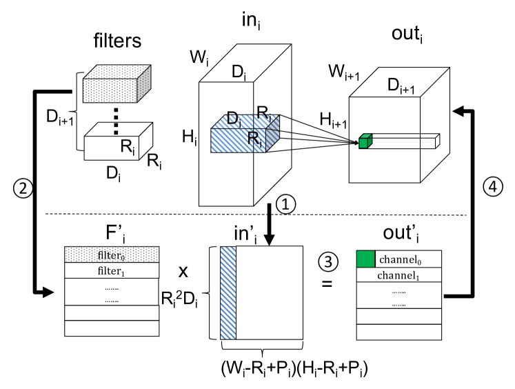
Figure 2: Mapping a convolutional layer (upper part of the figure) to a matrix multiplication (lower part).

The figure highlights a neuron in $out_{i}$ (right part of the upper row). The neuron is a result of a convolution operation – an elementwise dot product of the filter shaded in dots and the subvolume shaded in dashes. Both the subvolume and the filter have dimensions $R_{i}\times R_{i}\times D_{i}$. Applying a filter on the entire input volume ($in_{i}$) generates one channel of the output ($out_{i}$). Thus, the number of filters in $i$th layer ($D_{i+1}$) is the number of channels in the output volume.

The lower row of Figure 2 shows a common implementation that transforms the multiple convolution operations in a layer into a single matrix multiply. First, as shown in arrow ①, each subvolume in the input volume is stretched out into a column.The number of elements in the column is $D_{i}\times R_{i}^{2}$. For an input volume with dimensions $W_{i}\times H_{i}\times D_{i}$, there are $(W_{i}-R_{i}+P_{i})(H_{i}-R_{i}+P_{i})$ such columns in total, where $P_{i}$ is the amount of zero padding. We call this transformed input matrix $\mathsf{in}_{i}^{\prime}$.

Second, as shown in arrow ②, individual filters are similarly stretched out into rows, resulting in matrix $F_{i}^{\prime}$. The number of rows in $F_{i}^{\prime}$ is the number of filters in the layer. Then, the convolution becomes a matrix multiply: $\mathsf{out}_{i}^{\prime}=F_{i}^{\prime}\cdot\mathsf{in}_{i}^{\prime}$ (③ in Figure 2).

Finally, the $\mathsf{out}_{i}^{\prime}$ matrix is reshaped back to its proper dimensions of the $out_{i}$ volume (arrow ④). Each row of the resulting $\mathsf{out}_{i}^{\prime}$ matrix corresponds to one channel in the $out_{i}$ volume. The number of columns of the $\mathsf{out}_{i}^{\prime}$ matrix is $(W_{i}-R_{i}+P_{i})(H_{i}-R_{i}+P_{i})$, which is the size of one output channel, namely, $W_{i+1}\times H_{i+1}$.

Table 2 shows the number of rows and columns in the matrices involved.

Matrix	n_row	n_column
$\mathsf{in}_{i}^{\prime}$	$D_{i}\times R_{i}^{2}$	$(W_{i}-R_{i}+P_{i})(H_{i}-R_{i}+P_{i})$
$F_{i}^{\prime}$	$D_{i+1}$	$D_{i}\times R_{i}^{2}$
$\mathsf{out}_{i}^{\prime}$	$D_{i+1}$	$(W_{i}-R_{i}+P_{i})(H_{i}-R_{i}+P_{i})=W_{i+1}\times H_{i+1}$

Table 2: Matrix sizes in a convolutional layer.

The matrix multiplication described above processes a single input. As with fully-connected DNNs, CNN inference typically consumes a batch of $B$ inputs in a single forward pass. In this case, a convolutional layer performs $B$ matrix multiplications per pass. This is different from fully-connected layers, where the entire batch is computed using only one matrix multiplication.

4.2 Resolving DNN Hyper-parameters

Based on the previous analysis, we can now map DNN hyper-parameters to matrix operation parameters assuming all layers are sequentially connected.

4.2.1 Fully-connected networks

Consider a fully-connected network. Its hyper-parameters are the number of layers, the number of neurons in each layer ($N_{i}$) and the activation function per layer. As discussed in Section 4.1, the feed-forward computation performs one matrix multiplication per layer. Hence, we extract the number of layers by counting the number of matrix multiplications performed. Moreover, according to Table 1, the number of neurons in layer $i$ ($N_{i}$) is the number of rows of the layer’s weight matrix ($\theta_{i}$). Table 3 summarizes the mappings.

Structure	Hyper-Parameter	Value
FC network	# of layers	# of matrix muls
FC layeri	$N_{i}$: # of neurons	$n\_row(\theta_{i})$
Conv network	# of Conv layers	# of matrix muls / $B$
Conv layeri	$D_{i+1}$: # of filters	$n\_row(F_{i}^{\prime})$
	$R_{i}$:	$\sqrt{\frac{n\_row(in_{i}^{\prime})}{n\_row(out_{i-1}^{\prime})}}$
	filter width/height
	$P_{i}$: padding	compare:
		$n\_col(out_{i-1}^{\prime}),n\_col(in_{i}^{\prime})$
Pooli/	pool/stride	$\approx\sqrt{\frac{n\_col(out_{i}^{\prime})}{n\_col(in_{i+1}^{\prime})}}$
Stridei+1	width/height

Table 3: Mapping between hyper-parameters and matrix parameters. FC stands for fully connected.

4.2.2 Convolutional networks

A convolutional network generally consists of four types of layers: convolutional, Relu, pooling, and fully connected. Recall that each convolutional layer involves a batch $B$ of matrix multiplications. We determine $B$ with the following observation: consecutive matrix multiplications will have the same dimensions if they correspond to the same layer in a batch. We will see that this is the case below.

In a convolutional layer $i$, the hyper-parameters include the number of filters ($D_{i+1}$), the filter width or height ($R_{i}$), and the padding ($P_{i}$). We assume that the filter width and height are the same, which is the common case. Note that the depth of the input volume ($D_{i}$) is not considered; it is an input parameter, obtained from the previous layer.

From Table 2, we see that the number of filters ($D_{i+1}$) is the number of rows of the filter matrix $F_{i}^{\prime}$. To attain the filter width ($R_{i}$), we note that the number of rows of the $in_{i}^{\prime}$ matrix is $D_{i}\times R_{i}^{2}$. Hence, we first need to find $D_{i}$, which is the number of output channels in the previous layer. It can be obtained from the number of rows of the $out_{i-1}^{\prime}$ matrix. Overall, as summarized in Table 3, the filter width is attained by dividing the number of rows of $in_{i}^{\prime}$ by the number of rows of $out_{i-1}^{\prime}$ and performing the square root. In the case that the $i$th layer is the first one, directly connected to the input, the denominator of this fraction is the number of channels of the input image, which is public information.

Padding results in a larger input matrix ($in_{i}^{\prime}$). After resolving the filter width ($R_{i}$), the value of padding can be deduced by determining the difference between number of columns of the output matrix of layer $i-1$ ($out_{i-1}^{\prime}$), which is $W_{i}\times H_{i}$, and the number of columns of the $in_{i}^{\prime}$ matrix, which is $(W_{i}-R_{i}+P)(H_{i}-R_{i}+P)$.

A pooling layer can be located in-between two convolutional layers. It down-samples every channel of the input along width and height. The hyper-parameter in this layer is the pool width and height (assumed to be the same value), which can be inferred as follows. Consider first the (x,y) size of layer $i$, which is $W_{i+1}\times H_{i+1}$ (Table 2), and is given by the number of columns in matrix $out_{i}^{\prime}$. Then consider the (x,y) size of the input volume in layer $i+1$. If the two are the same, there is no pooling layer; otherwise, we expect to see the next (x,y) size reduced by the square of the pool width. In the latter case, the exact pool dimension can be found using a similar procedure used to determine $R_{i}$. Note that non-unit stride results in the same dimension difference, thus we are unable to distinguish these two.

Table 3 summarizes the mappings.

4.3 Connections Between Layers

We generalize the above mapping analysis by showing how to map inter-layer connections to GEMM execution.

4.3.1 Mapping shortcut/branch connections

A branch or shortcut path has two characteristics that can be expressed in GEMM execution. First, the sink (destination) of a shortcut or the merge point of a branch is mapped to a relatively longer inter-GEMM latency. Generally, DNNs perform the following operations between two consecutive GEMMs: post-processing the current GEMM’s output (e.g., batch normalization) and pre-processing the next GEMM’s input (e.g., padding and striding). Therefore, the inter-GEMM latency should be linearly related to the sum of the current layer’s output size and the next layer’s input size. However, at the sink, an extra element-wise matrix addition or subtraction needs to be performed, which incurs extra latency between consecutive GEMM calls. Second, the source of a shortcut or a branch must have the same output dimension as the sink. This is because a shortcut/branch only connects two layers whose output dimensions match. We find that these two characteristics are very useful in reducing the architecture search space.

4.3.2 Mapping consecutive connections

According to the mapping relationships in Table 3, a DNN places several constraints on GEMM parameters for consecutive convolutional layers. We can leverage these constraints to identify non-sequential connections. First, since filter width/height must be integer values, there is a constraint on the number of rows of the input and output matrix sizes between consecutive layers. Considering the formula used to derive filter width/height in Table 3, if layer $i-1$ and layer $i$ are consecutively connected, the number of rows in $i$th layer’s input matrix ($n\_row(in_{i})$) must be the product of the number of rows in the $i-1$th layer’s output matrix ($n\_row(out_{i-1})$) and square of an integer number. Second, since pool size and stride size are integer values, there is another constraint on the number of columns of the input and output matrix sizes between consecutive layers. According to the formula used to derive pool/stride size, if layer $i$ and layer $i+1$ are consecutively connected, the number of columns in $i$th layer’s output matrix ($n\_col(out_{i})$) must be the product of the number of columns in the $i+1$th layer’s input matrix ($n\_col(in_{i+1})$) and square of an integer number. The two constraints above can help us to locate non-sequential connections. Specifically, if one of these constraints is not satisfied, we are sure the two layers are not consecutively connected.

4.4 Activation Functions

So far, this section discussed how DNN parameters map to GEMM calls. Convolutional and fully-connected layers are post-processed by element-wise non-linear functions which do not appear in GEMM parameters. We can distinguish relu activations from sigmoid and tanh by monitoring a probe address in the sigmoid function using cache attacks. We remark that nearly all convolutional layers use relu or a close variant [35, 36, 37, 38, 2].

5 Attacking Matrix Multiply

We now design a side-channel attack to learn matrix multiplication parameters. Given the mapping from the previous section, this attack will allow us to reconstruct the DNN architecture.

We analyze state-of-the-art BLAS libraries, which have extensively optimized blocked matrix multiply for performance. Examples of such libraries are OpenBLAS [31], BLIS [39], Intel MKL [33] and AMD ACML [40]. We show in detail how to extract the desired information from the GEMM implementation in OpenBLAS. In Section 6, we generalize our attack to other BLAS libraries, using Intel MKL as an example.

5.1 Analyzing GEMM from OpenBLAS

Function gemm_nn from the OpenBLAS library performs blocked matrix-matrix multiplication. It computes $C=\alpha A\cdot B+\beta C$ where $\alpha$ and $\beta$ are scalars, A is an m $\times$ k matrix, B is a k $\times$ n matrix, and C is an m $\times$ n matrix. Our goal is to extract m, n and k.

Like most modern BLAS libraries, OpenBLAS implements the Goto’s algorithm [41]. Such algorithm has been optimized for modern multi-level cache hierarchies and CPUs. Figure 3 depicts the way the Goto’s algorithm structures blocked matrix multiplication for a three-level cache.

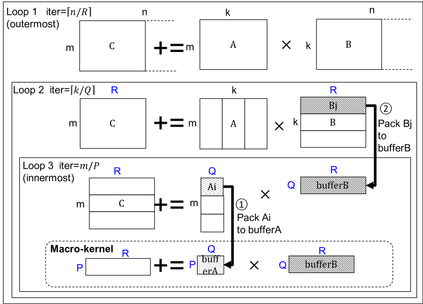
Figure 3: Blocked GEMM with matrices in column major.

The macro-kernel at the bottom performs the basic operation, multiplying a P $\times$ Q block from matrix A with a Q $\times$ R block from matrix B. This kernel is generally written in assembly code, and manually optimized by taking CPU pipeline structure and register availability into consideration. The block sizes are picked so that the P $\times$ Q block of A fits in the L2 cache, and the Q $\times$ R block of B fits in the L3 cache.

As shown in Figure 3, there is a three-level loop nest around the macro-kernel. The innermost one is Loop 3, the intermediate one is Loop 2, and the outermost one is Loop 1. We call the iteration counts in these loops $iter_{3}$, $iter_{2}$, and $iter_{1}$, respectively, and are given by:

$$iter_{3}=\lceil m/P\rceil;\quad iter_{2}=\lceil k/Q\rceil;\quad iter_{1}=\lceil n/R\rceil$$ (1)

Algorithm 1 shows the corresponding pseudo-code with the three nested loops. Note that, Loop 3 is further split into two parts, to obtain better cache locality. The first part performs only the first iteration, and the second part performs the rest.

Input : Matrix $A$, $B$, $C$; Scalar $\alpha$, $\beta$; Block size $P,Q,R$; $UNROLL$

Output : $C:=\alpha A\cdot B+\beta C$

1 for $j=0,n,R$ do // Loop 1

2       for $l=0,k,Q$ do // Loop2

3             $itcopy(A[0,l],buf\_A,P,Q)$

             // Loop 3, 1st iteration

4             for $jj=j,j+R,3UNROLL$ do

5                   $oncopy(B[l,jj],buf\_B+(jj-j)\times Q,Q,3UNROLL)$

6                   $kernel(buf\_A,buf\_B+(jj-j)\times Q,C[l,j],P,Q,3UNROLL)$

7             end for

8            for $i=P,m,P$ do // Loop 3, rest iterations

9                   $itcopy(A[i,l],buf\_A,P,Q)$

10                   $kernel(buf\_A,buf\_B,C[l,j],P,Q,R)$

11             end for

12            

13       end for

14      

15 end for

Algorithm 1 gemm_nn in OpenBLAS

In all the iterations of Loop 3, the data in the P $\times$ Q block from matrix A is packed into a buffer (function itcopy), before calling the macro-kernel (function kernel). This is shown in Figure 3 as arrow ① and corresponds to Line 3 and 9 in Algorithm 1. Additionally, in the first part of Loop 3, the data in the Q $\times$ R block from matrix B is also packed into a buffer (function oncopy). This is shown in Figure 3 as arrow ② and corresponds to Line 5 in Algorithm 1. The Q $\times$ R block from matrix B is copied in units of Q $\times$ 3UNROLL sub-blocks.This breaks down the first part of Loop 3 into a loop with an iteration count of $iter_{4}$, given by:

$$\begin{split}&iter_{4}=\lceil R/3UNROLL\rceil\\ or\quad&iter_{4}=\lceil(n\bmod R)/3UNROLL\rceil\end{split}$$ (2)

where the second expression corresponds to the last iteration of Loop 1.

5.2 Locating Probing Addresses

Our goal is to find the size of the matrices of Figure 3, namely, m, k, and n. To do so, we need to first obtain the number of iterations of Loops 1, 2, and 3, and then use Equation 1. Note that we know the values of the block sizes P, Q, and R (as well as UNROLL) — these are constants available in the open-source code of OpenBLAS.

A straight-forward approach to obtain the number of iterations of Loops 1, 2, and 3 is to monitor the addresses that hold the instructions of the loop entries. These are Lines 1, 2, and 8 in Algorithm 1, respectively. We could count the number of times these instructions are executed. However, this fails because the loop body is very tight. Specifically, the instructions for Lines 1 and 2 fall into the same cache line, and Line 8 falls into a cache line that is very close to them. To disambiguate all the loops, we need to monitor better addresses.

In this paper, we propose to use, as probing addresses, addresses in the itcopy, oncopy and kernel functions of Algorithm 1. To understand why, consider the dynamic invocations to these functions. Figure 4 shows the Dynamic Call Graph (DCG) of gemm_nn in Algorithm 1. Each iteration of Loop 2 contains one invocation of function itcopy, followed by $iter_{4}$ invocations of the pair oncopy and kernel, and then $(iter_{3}-1)$ invocations of the pair itcopy and kernel. The whole sequence in Figure 4 is executed $iter_{1}\times iter_{2}$ times in one invocation of gemm_nn.

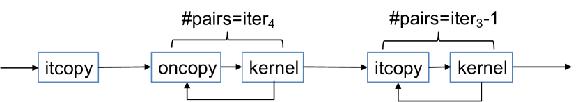
Figure 4: DCG of gemm_nn, with the number of invocations per iteration of Loop 2.

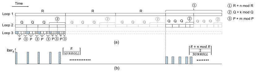
Figure 5: Visualization of execution time of gemm_nn where Loop 1, Loop 2, and Loop3 have 5 iterations each (a); value of $iter_{4}$ for each first-iteration of Loop 3 (b).

We will see in Section 5.3 that these invocation counts are enough to allow us to find the size of the matrices of Figure 3. However, using the first instruction in itcopy, oncopy, and kernel as probe addresses is not optimal. Indeed, we have found that these instructions are sometimes accessed by prefetchers in the shadow of a branch misprediction. This introduces noise in the measurements.

Alternatively, we use one instruction inside each function for the three probe addresses. Further, since the main bodies of these functions are loops, we use instructions that are part of the loop (to distinguish it from the GEMM loops, we call it in-function loop). This improves our monitoring capability, as such instructions are accessed multiple times per function invocation.

Overall, instructions in the bodies of these three functions satisfy the conditions for good probing addresses. First, we will see that the number of accesses to these instructions can be used to deduce the iteration count of each level of the loop. Second, these addresses are distant from each other and, hence, automatic prefetching of instructions does not introduce noise. Finally, since each function operates on a block of data, the intervals between consecutive invocations of these functions are long enough.

Note that, even though this DCG is specific for gemm_nn in OpenBLAS, it captures two common features for general blocked matrix multiplication. First, all implementations use a kernel function as a unit to carry out block-size computation. Second, there are always packing operations before kernel execution at two different levels of the loop. A similar DCG can be extracted for slightly different implementations, such as Intel’s MKL (Section 6).

5.3 Procedure to Extract Matrix Dimensions

To understand the procedure we use to extract matrix dimensions, we note the way OpenBLAS groups blocks into iterations. Specifically, rather than assigning a small block to the last iteration, it assigns two equal-sized small blocks to the last two iterations. For example, as it blocks the n columns of matrix C in Figure 3 into blocks of size R, it assigns R columns to each Loop 1 iteration, except for the last two iterations. Each of the latter receives (R + n mod R)/2.

Figure 5(a) shows the visualization of the execution time of gemm_nn where Loop 1, Loop 2, and Loop 3 have 5 iterations each. It shows the size of the block each iteration operates on. In Loop 1, the first three iterations use R-sized blocks; each of the last two use a block of size (R + n mod R)/2. In Loop 2, the corresponding block sizes are Q and (Q + k mod Q)/2. In Loop 3, they are P and (P + m mod P)/2.

Recall that the first iteration of every Loop 3 invocation is special. While it processes a P-sized block, its execution time is different because it performs a different operation. Specifically, as shown in Figure 4, it invokes the oncopy-kernel pair $iter_{4}$ times. Figure 5(b) shows the value of $iter_{4}$ for each of the first iterations of Loop 3. As indicated in Equation 2, during the execution of “normal” Loop 1 iterations, it is $\lceil R/3UNROLL\rceil$. However, in the last two iterations of Loop 1, $iter_{4}$ is $\lceil((R+nmodR)/2)/3UNROLL\rceil$.

Based on these insights, our procedure to extract m, k, and n has four steps.

Step 1: Identify the DCG of Loop 2 iterations, and extract $iter_{1}\times iter_{2}$. By probing one instruction in each of itcopy, oncopy, and kernel, we repeatedly obtain the DCG pattern of Loop 2 iterations (Figure 4). By counting the number of such patterns, we obtain $iter_{1}\times iter_{2}$.

Step 2: Extract $iter_{3}$ and determine the value of $m$. In the DCG pattern of a Loop 2 iteration, we count the number of invocations to the itcopy-kernel pair (Figure 4). This count plus 1 gives $iter_{3}$. Of all these $iter_{3}$ iterations, all but the last two execute a block of size P; the last two execute a block of size (P + m mod P)/2 each (Figure 5(a)). To estimate the size of this smaller block, we assume that the execution time of an iteration is proportional to the block size it processes — except for the first iteration which, as we indicated, is different. Hence, we time the execution of a “normal” iteration of loop L3 and the execution of the last iteration of Loop 3. Let’s call the times $t_{normal}$ and $t_{small}$. The value of $m$ is:

$$m=(iter_{3}-2)\times P+2\times\frac{t_{small}}{t_{normal}}\times P\vspace{-2pt}$$

Step 3: Extract $iter_{4}$, $iter_{2}$ and determine the value of $k$. In the DCG pattern of a Loop 2 iteration (Figure 4), we count the number of oncopy-kernel pairs, and obtain $iter_{4}$. As shown in Figure 5(b), the value of $iter_{4}$ is $\lceil R/3UNROLL\rceil$ in all iterations of Loop 2 except those that are part of the last two iterations of Loop 1. For the latter, $iter_{4}$ is $\lceil((R+nmodR)/2)/3UNROLL\rceil$, which is a lower value. Consequently, by counting the number of DCG patterns that have a low value of $iter_{4}$, and dividing it by 2, we attain $iter_{2}$. We then follow the procedure of Step 2 to calculate k. Specifically, all Loop 2 iterations but the last two execute a block of size Q; the last two execute a block of size (Q + k mod Q)/2 each (Figure 5(a)). Hence, we time the execution of a “normal” iteration and the last one, and compute $k$ as per Step 2.

Step 4: Extract $iter_{1}$ and determine the value of $n$. If we count the total number of DCG patterns in the execution and divide that by $iter_{2}$, we obtain $iter_{1}$. We know that all Loop 1 iterations but the last two execute a block of size R; the last two execute a block of size (R + n mod R)/2 each. To compute the latter, we note that, in the last two iterations of Loop 1, $iter_{4}$ is $\lceil((R+nmodR)/2)/3UNROLL\rceil$. Since both $iter_{4}$ and $3UNROLL$ are known, we can compute (R + n mod R)/2. Hence, the value of $n$ is:

$$n=(iter_{1}-2)\times R+2\times iter_{4}\times 3UNROLL$$

However, our attack cannot handle the case when the matrix dimension size is less than twice the block size — for example, when n is less than $2\times R$. In this case, there is no iteration that works on a full block. Our procedure cannot compute the exact value of n, and can only provide a range of values.

6 Generalization of the Attack

Our attack can be generalized to other BLAS libraries, since all of them use blocked matrix-multiplication, and most of them implement Goto’s algorithm [41]. Even though they may differ in the scheduling of the three-level nested loop, block sizes and implementation of the macro-kernel, our attack is still effective. In this section, we show that the same attack strategy can be applied to other BLAS libraries, using Intel MKL as an example. We choose MKL for two reasons. First, it is another heavily used library (similar to OpenBLAS). Second, it is closed source, which makes the attack more challenging.

Since MKL’s source code is not disclosed, we need to complete two tasks before extracting matrix parameters. First, we need to construct the DCG of GEMM using packing and kernel functions. This requires us to find the proper functions and their invocation patterns. Second, we need to obtain the block size of each dimension. In both tasks, we leverage side channel attacks to assist program analysis.

Constructing the DCG

First, we use GDB to manually analyze the binary code. We trace down the functions that are called during matrix multiplication, which we find are the packing functions copybn, copyan. We find that the kernel function is called ker0.

Next, we determine function invocation patterns and correlate those patterns with loop executions. This can be achieved in multiple ways. One possible approach is manual analysis, that is, using GDB to trace the dynamic execution path of GEMM and observe the functions invoked for each loop. Another approach is leveraging cache-based side channel attacks to probe the packing and kernel functions, and obtain the invocation patterns.

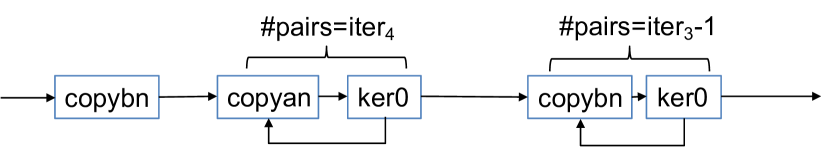
Figure 6: DCG of blocked GEMM in Intel MKL, with the number of invocations per iteration of Loop 2.

We derive the same DCG using the two approaches, shown in Figure 6. The pattern is the same as the DCG of OpenBLAS in Figure 4. Thus, the attack strategy in Section 5 should also work towards MKL.

Extracting block sizes

According to Formulas 1 and  2, there is a discrete linear relationship between the matrix size and the iteration count. We leverage the side-channel attacks in Section 5 to count the number of iterations and resolve block sizes. Specifically, we gradually increase the input dimension size until the number of iterations increments. For each dimension, the stride on the input dimension that triggers the change of iteration count is the block size. By applying this approach, we can successfully derive block sizes, which match the sizes we obtain via manual analysis of the MKL binary code.

Special cases

According to our analysis, MKL follows a different DCG when dealing with small matrices. Instead of doing 3-level nested loops as in Figure 6, it uses a single-level loop, tiling on the dimension that has the largest value among $m$, $n$, $k$. The computation is done in place, without triggering packing functions. For these special cases, we slightly adjust the attack strategy in Figure 5. We use side channels to monitor the number of iterations on that single-level loop and the time spent for each iteration. We then use the number of iterations to deduce the size of the largest dimension. Finally, we use the timing information for each iteration to deduce the product of the other two dimensions.

7 Experimental Setup

Attack Platform

We evaluate our attacks on a Dell workstation Precision T1700, which has a 4-core Intel Xeon E3 processor and an 8GB DDR3-1600 memory. The processor has two levels of private caches and a shared last level cache. The first level caches are a 32KB instruction cache and a 32KB data cache. The second level cache is 256KB. The shared last level cache is 8MB. We test our attacks on a same-OS scenario using Ubuntu 4.2.0-27. Our attacks should be applicable to other platforms, as the effectiveness of Flush+Reload and Prime+Probe has been proved in multiple hardware platforms [18, 17].

Victim DNNs

We use a VGG [37] instance and a ResNet [2] instance as victim DNNs. VGG is representative of early DNNs (e.g., AlexNet [36] and LeNet [42]). ResNet is representative of state-of-the-art DNNs. Both are standard and widely-used CNNs with a large number of layers and hyper-parameters. ResNet additionally features shortcut/branch connections (Section 4.3). There are several versions of VGG, with 11 to 19 layers. All VGGs contain 5 blocks and, within each block, a single type of layer is replicated. We show our results on VGG-16. There are several versions of ResNet, whose depth varies from 18 to 152 layers. All of them consist of the same 4 types of modules, which are replicated a different number of times. Each module contains 3 or 4 layers, which are all different. We show our detection results on ResNet-50. The victim programs are implemented using the Keras [43] framework, with Theano [34] as the backend.

8 Evaluation

We first evaluate our attacks on the GEMM function. We then show the effectiveness of our attack on neural network inference. We provide a detailed analysis of extracting the DNN architecture for a VGG-16 and a ResNet-50 instance, and quantify the reduction in the architecture search space.

8.1 Attacking GEMM Using Prime+Probe

We show the results of attacking GEMM using Prime+Probe, which does not require page sharing or the use of the clflush instruction. Our attack targets the LLC. Hence, victim and attacker can run on different cores, further improving the attack’s flexibility. We locate the LLC sets of two instructions from itcopy and oncopy, and construct two sets of eviction addresses using the algorithm proposed by Liu et al. [18].

Figure 7 shows one raw trace of the execution of one iteration of Loop 2 in Algorithm 1. We only show the latency above $500$ cycles, which indicates victim activities. Note that, since we select the probe addresses to be within loop bodies (Section 5.2), a cluster of misses marks the time period when the victim is executing the probed function. In this trace, the victim calls itcopy around interval 2000, then calls oncopy $11$ times between intervals 2000 and 7000. It then calls itcopy another two times in intervals 7000 and 13000. The trace matches the DCG shown in Figure 4, and we can derive that $iter_{4}=11$ and $iter_{3}=3$.

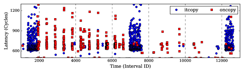
Figure 7: Prime+Probe trace of the GEMM execution with monitoring interval length equal to 2000 cycles.

The noise, such as between intervals 8000 and 12000, can be trivially distinguished from the actual victim accesses. The trace can be further cleaned up by leveraging de-noising techniques [18],[17]. As Prime+Probe can effectively extract matrix parameters and achieve the same high accuracy as Flush+Reload, either can be used to extract DNN hyper-parameters. Thus, in the rest of this section, we use Flush+Reload to illustrate our attack.

8.2 Extracting Parameters from DNNs

We show the effectiveness of our attack by extracting the hyper-parameters of our VGG [37] and ResNet [2] instances. Figure 8 shows the extracted values of the $n$, $k$, and $m$ matrix parameters for the layers in the 4 distinct modules in ResNet-50, and for the first layer in each of the 5 blocks in VGG-16. We do not show the other layers because they are duplicates of the layers shown. Figures 8(a), (b), and (c) correspond to the values of $n$, $k$, and $m$, respectively.

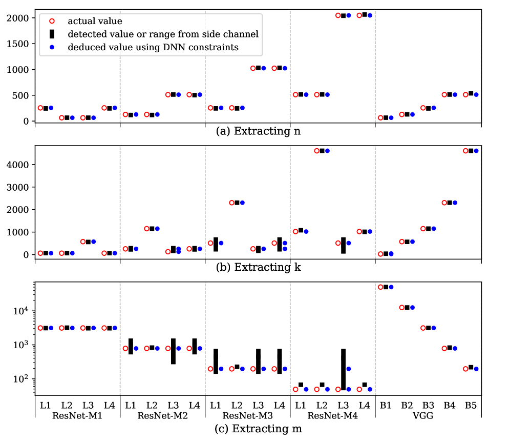
Figure 8: Extracted values of the $n$, $k$, and $m$ matrix parameters for VGG-16 and ResNet-50.

In Figure 8, for a given parameter (e.g., $m$) and a given layer (e.g., L1 in ResNet-M2), the hollowed circles indicate the actual value of the parameter. The squares or rectangles indicate the values of the parameters detected with the side channel attack. When the side channel attack can only narrow down the possible values to a range, the figure shows a rectangle. Finally, the solid circles indicate the values of the parameters that we deduce, using the detected values and some DNN constraints. For example, for parameter $m$ in layer L1 of ResNet-M2, the actual value is 784, the detected value range is 524-1536, and the deduced value is 784.

We will discuss how we obtain the solid circles later. Here, we focus on comparing the actual and detected values (hollowed circles and squares/rectangles). Figure 8(a) shows that our attack is always able to determine the $n$ dimension size with ignorable error, thanks to the small subblock size used in the 1st iteration of Loop 3 (Algorithm 1).

Figures 8(b) and (c) show that the attack is able to accurately determine the $m$ and $k$ values for most layers in ResNet-M1, ResNet-M4 and all blocks in VGG. However, it can only derive ranges of values for most of the ResNet-M2 and ResNet-M3 layers. This is because the $m$ and $k$ values in these layers are often smaller than twice the corresponding block sizes (Section 5.3).

In summary, our side channel attack can either detect the matrix parameters with negligible error, or can provide a range where the actual value falls in. We will later show that the imprecision from the negligible error and the ranges can be eliminated after applying DNN constraints.

8.3 Size of Architecture Search Space

The goal of Cache Telepathyis to very substantially reduce the search space of possible architectures that can match the oracle architecture. In this section, we compare the number of architectures in the search space without Cache Telepathy (which we call Original space), and with Cache Telepathy. In both cases, we initially reduce the search space by only considering reasonable hyper-parameters for the layers. Specifically, for convolutional layers, the number of filters can be a multiple of $64$ ($64\times i$, where $1\leq i\leq 32$), and the filter size can be an integer value between $1$ and $11$. For fully-connected layers, the number of neurons can be $2^{i}$, where $8\leq i\leq 13$.

8.3.1 Size of the original search space

To be conservative, we assume that the attacker knows the number of layers and type of each layer in the oracle DNN. There exist $352$ different configurations for each convolutional layer without considering pooling or striding, and $6$ configurations for each fully-connected layer. Moreover, considering the existence of branches, given $L$ layers, there are $L\times 2^{L-1}$ possible ways to connect them.

If we do not count potential shortcuts or branches, a network with 13 convolutional layers and 3 fully-connected layers such as VGG-16 has a search space size of about $4\times 10^{35}$. If we consider non-sequential connections, for a network module with only 4 convolutional layers such as Module 1 in ResNet-50, there are around $5\times 10^{11}$ possible architectures. Considering that ResNet-50 has 4 different modules, the total search space will be over $5.8\times 10^{46}$. The search space would be even larger in an actual attack scenario, since the attacker would not have any information on the total number of layers and layer types.

Overall, we can see that the search space is intractable. Since training each candidate DNN architecture takes hours to days, relying on the original search space does not lead to obtaining the oracle DNN architecture.

8.3.2 Determining the reduced search space

Using the detected values of the matrix parameters in Section 8.2, we first determine the possible connections between layers by locating shortcuts/branches and non-sequential connections. For each possible connection configuration, we calculate the possible hyper-parameters for each layer. The final search space is computed as

$$search\ space=\sum_{i=1}^{C}{(\prod_{j=1}^{L}{x_{j}}})$$ (3)

where $C$ is the total number of possible connection configurations, $L$ is the total number of layers, and $x_{j}$ is the number of possible combinations of hyper-parameters for layer $j$.

Determining connections between layers

We first try to determine the connections between layers. As discussed in Section 4.3, we can leverage the inter-GEMM latency to determine the sink of a shortcut or a branch. Figure 9 shows the extracted input and output matrix sizes, and the inter-GEMM latencies for the layers in ResNet_M1. The inter-GEMM latency for M1_L4 is significantly larger than expected, given its corresponding input and output matrix sizes, and thus can be identified as a sink. Using the extracted dimension information (values of $n$ and $m$) in Figure 8, we determine that only M1_L1 matches the output matrix size of M1_L4. Therefore, we know that M1_L1 is the source. Further, by applying the DNN constraints on consecutive layers (Section 4.3), we find that M1_L1 and M1_L2 are not consecutively connected, because $m_{M1\_L2}$ cannot be the product of $n_{M1\_L1}$ and the square of an integer.

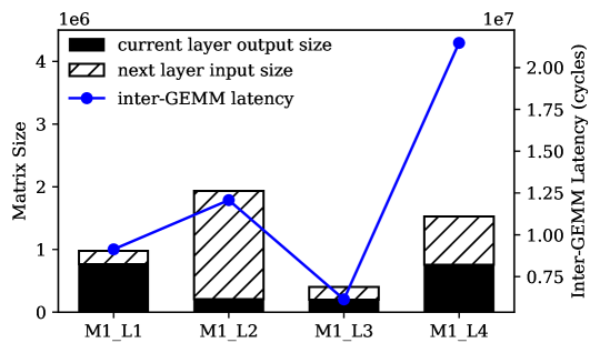
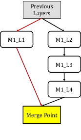
Figure 9: Extracting connections between layers in ResNet_M1.

Based on the analysis above, we reverse engineer the connections among the 4 layers, as shown in Figure 9. These connections exactly match the actual ones in ResNet. We use the same method to derive the possible connection configurations for the other modules.

Determining hyper-parameters for each layer

We plug the detected matrix parameters into the formulas in Table 3 to deduce the hyper-parameters for each layer. For those matrix parameters that cannot be extracted precisely, we leverage DNN constraints to prune the search space, as discussed in Section 4.3. For example, for convolutional layers, we use the $n$ and $k$ dimensions between two consecutive layers to deduce the number of filters and the filter sizes.

As an example, consider L3 in ResNet_M3. First, we round the extracted $n$ to the nearest multiple of 64 to get 512, which is the number of filters in that layer. Since we only have a very small error when detecting the $n$ dimension, we always obtain the correct number of filters in Figure 8(a). Second, we use the formula in Table 3 to determine the filter size. The value for $n_{M2\_L2}$ is $118$, but we cannot determine the value for $k_{M2\_L3}$. As discussed in Section 4.3, for consecutive layers, the $k$ dimension of the current layer must be the product of the $n$ dimension of the last layer and the square of an integer. Considering that $k_{M2\_L3}$ is within the range $[68,384]$, the only possible value is $118$. In this way, we successfully reduce the parameter range to a single value, and deduce that the filter size is 1.

We apply the same methodology for the other layers. With this method, we obtain the solid circles in Figure 8. In some cases, this methodology generates two possible deduced values. For example, this happens for the $k$ parameter in ResNet_M3 Layer 4. In this case, we have two solid circles in Figure 8, and we have to consider both architectures.

Determining pooling/striding

We use the differences in the $m$ dimension between consecutive layers to determine the pool or stride size. For example, we see that the $m$ dimension changes from ResNet_M1 to ResNet_M2. Even though we cannot precisely determine the value of $m_{M2\_L1}$, we can use DNN constraints to reduce the possible number of pooling/striding sizes. As discussed in Section 4.3, the reduction in the $m$ dimension must be the square of an integer. Since $m_{M1\_L4}=3072$ and $m_{M2\_L1}$ is within the range $[524,1536]$, we can deduce that $m_{M2\_L1}$ is $768$ and that the pool/stride size is $2$. Since we cannot distinguish between pool layers and stride operations, we still have two possible configurations in the final search space: one with a pool layer, and one with a stride operation.

8.3.3 The size of the reduced search space

Based on the previous discussion, Table 4 shows the original size of the search space, and the reduced one after using Cache Telepathy. Recall that we calculate the original space assuming that the attacker already knows the total number of layers and the type of layers, which is a conservative assumption.

DNN	Original: No	Using Cache Telepathy
	Side Channel	OpenBLAS	MKL
ResNet-50	$>5.8\times 10^{46}$	512	6144
VGG-16	$>4\times 10^{35}$	16	64

Table 4: Comparing the original and reduced search spaces.

Using Cache Telepathy, we are able to significantly reduce the search space from an intractable size to a reasonable size. The reduced search space is smaller in the VGG network because of its relatively small number of layers. Further, our attacks on MKL are less effective than on OpenBLAS. This is because the matrix sizes in ResNet_M4 are small, and MKL handles these matrices specially (Section 6). Even after applying DNN constraints, we can only limit the number of possible values for some parameters in each layer of that module to $2$ or $4$, which leads to the wider space size.

9 Countermeasures

We overview possible countermeasures against our attack, and discuss their effectiveness and performance implications.

Since our attack targets BLAS libraries, we first investigate whether it is possible to stop the attack by modifying the libraries. One approach is to use less aggressive optimization. It is unfeasible to abandon blocking completely, since unblocked matrix multiplication has poor cache performance. However, it is possible to use a less aggressive blocking, with tolerable performance degradation. Specifically, we can remove the optimization for the first iteration of Loop 3 (Lines 4-7 in Algorithm 1). In this case, it will be difficult for the attacker to precisely recover the values of $n$ and $k$ without a much more detailed timing analysis.

Another approach is to reduce the sizes of the dimensions of the matrices. If the sizes of two or more dimensions of a matrix are smaller than the block size, the attacker can only obtain ranges for the values of those dimensions. This makes the attack much harder. There are existing techniques to reduce the sizes of the dimensions of a matrix. For example, linear quantization reduces the weight and input precision, which means that the matrix becomes smaller. This mitigation is typically effective for the last few layers in a convolutional network, which use relatively small matrices. However, it cannot protect layers with large matrices, such as those using a large number of filters and input activations.

Alternatively, one can use existing cache-based side channel defense mechanisms. One approach is to disallow resource sharing. For example, the MLaaS provider can disallow server sharing between different users. However, this is an extreme solution with major disadvantages in throughput. Another approach is to disable page sharing and page de-duplication. Unfortunately, while this defeats the Flush+Reload attack, it does not defeat Prime+Probe.

Another approach is to use cache partitioning, such as Intel CAT (Cache Allocation Technology), which assigns different ways of the LLC to different applications [44]. Since attackers may also target data access patterns, both code and data need to be protected in the cache. This means that the GEMM block size needs to be adjusted to the reduced number of available ways in the LLC. There will be some performance degradation due to reduced LLC capacity, but this is likely a good trade-off between performance and security.

Further, there are proposals for security-oriented cache mechanisms such as PLCache [45], Random Fill Cache [46], SHARP [47] and SecDCP [48]. If these mechanisms are adopted in production hardware, they can mitigate our attack with moderate performance degradation. Finally, one can add security features to performance-oriented cache partitioning proposals [49],[50],[51],[52], to achieve better trade-offs between security and performance.

10 Related Work

Recent research has called attention to the confidentiality of ML hyper-parameters. Hua et al. [53] designed the first attack to steal CNN architectures running on a hardware accelerator. Their attack is based on a different threat model, which requires the attacker to be able to monitor all of the memory accesses issued by the victim, including the type and address of each access. Our attack does not require such elevated privilege.

Cache-based side channel attacks have been used to trace program execution to steal sensitive information. However, there is no existing cache-based side channel attack that can achieve the goal of extracting all the hyper-parameters of a DNN, given the complexity of DNN computations, and the multi-level loop structure of GEMM, as well as the high number of parameters to extract. Most side channel attacks target cryptography algorithms, such as AES [54, 19, 55], RSA [18, 17] and ECDSA [56]. These attacks directly correlate binary bits within the secret key with either branch execution or matrix location access. Our attack on GEMM requires careful selection of probing addresses, and complicated post-analysis. Furthermore, our attack can extract a much higher number of hyper-parameters, instead of a secret key.

GEMM is an important application in high-performance computing, and there is a popular line of research on improving the memory hierarchy performance of GEMM (e.g., [57],[58],[59]).

11 Conclusion

In this paper, we proposed Cache Telepathy: a fast and accurate mechanism to steal a DNN’s architecture using cache-based side channel attacks. We identified that DNN inference relies heavily on blocked GEMM, and provided a detailed security analysis of this operation. We then designed an attack to extract the input matrix parameters of GEMM calls, and scaled this attack to complete DNNs. We used Prime+Probe and Flush+Reload to attack VGG and ResNet DNNs running OpenBLAS and Intel MKL libraries. Our attack is effective in helping obtain the architectures by very substantially reducing the search space of target DNN architectures. For example, for VGG using OpenBLAS, it reduced the search space from more than $10^{35}$ architectures to just 16.

References

- [1] Y. Wu, M. Schuster, Z. Chen, Q. V. Le, M. Norouzi, W. Macherey, M. Krikun, Y. Cao, Q. Gao, K. Macherey, J. Klingner, A. Shah, M. Johnson, X. Liu, L. Kaiser, S. Gouws, Y. Kato, T. Kudo, H. Kazawa, K. Stevens, G. Kurian, N. Patil, W. Wang, C. Young, J. Smith, J. Riesa, A. Rudnick, O. Vinyals, G. Corrado, M. Hughes, and J. Dean, “Google’s neural machine translation system: Bridging the gap between human and machine translation,” CoRR, vol. abs/1609.08144, 2016.
- [2] K. He, X. Zhang, S. Ren, and J. Sun, “Deep residual learning for image recognition,” CoRR, vol. abs/1512.03385, 2015.
- [3] A. Radford, L. Metz, and S. Chintala, “Unsupervised representation learning with deep convolutional generative adversarial networks,” CoRR, vol. abs/1511.06434, 2015.
- [4] D. Silver, A. Huang, C. J. Maddison, A. Guez, L. Sifre, G. van den Driessche, J. Schrittwieser, I. Antonoglou, V. Panneershelvam, M. Lanctot, S. Dieleman, D. Grewe, J. Nham, N. Kalchbrenner, I. Sutskever, T. Lillicrap, M. Leach, K. Kavukcuoglu, T. Graepel, and D. Hassabis, “Mastering the game of Go with deep neural networks and tree search,” Nature, vol. 529, pp. 484–489, Jan. 2016.
- [5] “Amazon machine learning.” https://aws.amazon.com/machine-learning/.
- [6] “Google machine learning.” https://cloud.google.com/products/machine-learning/.
- [7] F. Tramèr, F. Zhang, A. Juels, M. K. Reiter, and T. Ristenpart, “Stealing machine learning models via prediction apis,” in USENIX Security, 2016.
- [8] R. Shokri, M. Stronati, and V. Shmatikov, “Membership inference attacks against machine learning models,” arXiv preprint arXiv:1610.05820, 2016.
- [9] Y. Long, V. Bindschaedler, L. Wang, D. Bu, X. Wang, H. Tang, C. A. Gunter, and K. Chen, “Understanding membership inferences on well-generalized learning models,” CoRR, vol. abs/1802.04889, 2018.
- [10] K. Hazelwood, S. Bird, D. Brooks, S. Chintala, U. Diril, D. Dzhulgakov, M. Fawzy, B. Jia, Y. Jia, A. Kalro, J. Law, K. Lee, J. Lu, N. Pieter, S. Misha, X. Liang, and X. Wang, “Applied machine learning at facebook: A datacenter infrastructure perspective,” in International Symposium on High-Performance Computer Architecture (HPCA), IEEE, 2018.
- [11] Amazon, “Amazon sagemaker ml instance types,” 2018.
- [12] Y. LeCun, Y. Bengio, and G. Hinton, “Deep learning,” nature, vol. 521, no. 7553, p. 436, 2015.
- [13] C. De Sa, M. Feldman, C. Ré, and K. Olukotun, “Understanding and optimizing asynchronous low-precision stochastic gradient descent,” in ACM SIGARCH Computer Architecture News, vol. 45, pp. 561–574, ACM, 2017.
- [14] Wikipedia, “Hyperparameter optimization,” 2018.
- [15] J. Jordan, “Hyperparameter tuning for machine learning models,” 2017.
- [16] B. Wang and N. Z. Gong, “Stealing hyperparameters in machine learning,” in IEEE Symposium on Security and Privacy (SP), IEEE, 2018.
- [17] Y. Yarom and K. Falkner, “FLUSH+RELOAD: a high resolution, low noise, L3 cache side-channel attack,” in Proceedings of the 23rd USENIX Conference on Security Symposium, (Berkeley, CA, USA), pp. 719–732, USENIX Association, 2014.
- [18] F. Liu, Y. Yarom, Q. Ge, G. Heiser, and R. B. Lee, “Last-level cache side-channel attacks are practical,” in Proceedings of the 2015 IEEE Symposium on Security and Privacy, (Washington, DC, USA), pp. 605–622, IEEE Computer Society, 2015.
- [19] M. Neve and J. P. Seifert, “Advances on access-driven cache attacks on AES,” in Proceedings of the 13th International Conference on Selected Areas in Cryptography, (Berlin, Heidelberg), pp. 147–162, Springer-Verlag, 2007.
- [20] T. Hornby, “Side-channel attacks on everyday applications: distinguishing inputs with FLUSH+RELOAD.” https://www.blackhat.com/docs/us-16/materials/us-16-Hornby-Side-Channel-Attacks-On-Everyday-Applications-wp.pdf, 2016. Accessed on 22 April 2017.
- [21] M. Lipp, M. Schwarz, D. Gruss, T. Prescher, W. Haas, S. Mangard, P. Kocher, D. Genkin, Y. Yarom, and M. Hamburg, “Meltdown,” arXiv preprint arXiv:1801.01207, 2018.
- [22] P. Kocher, D. Genkin, D. Gruss, W. Haas, M. Hamburg, M. Lipp, S. Mangard, T. Prescher, M. Schwarz, and Y. Yarom, “Spectre attacks: Exploiting speculative execution,” arXiv preprint arXiv:1801.01203, 2018.
- [23] D. Skarlatos, N. S. Kim, and J. Torrellas, “Pageforge: a near-memory content-aware page-merging architecture,” in Proceedings of the 50th Annual IEEE/ACM International Symposium on Microarchitecture, pp. 302–314, ACM, 2017.
- [24] T. Ristenpart, E. Tromer, H. Shacham, and S. Savage, “Hey, you, get off of my cloud: exploring information leakage in third-party compute clouds,” in Proceedings of the 16th ACM Conference on Computer and Communications Security, (New York, NY, USA), pp. 199–212, ACM, 2009.
- [25] Y. Zhang, A. Juels, M. K. Reiter, and T. Ristenpart, “Cross-tenant side-channel attacks in PaaS clouds,” in Proceedings of the 2014 ACM SIGSAC Conference on Computer and Communications Security, (New York, NY, USA), pp. 990–1003, ACM, 2014.
- [26] Amazon, “Amazon sagemaker,” 2018.
- [27] Google, “Cloud ml engine overview,” 2018.
- [28] M. Abadi, P. Barham, J. Chen, Z. Chen, A. Davis, J. Dean, M. Devin, S. Ghemawat, G. Irving, M. Isard, et al., “Tensorflow: A system for large-scale machine learning,” in Proceedings of the 12th USENIX Symposium on Operating Systems Design and Implementation (OSDI). Savannah, Georgia, USA, 2016.
- [29] Y. Jia, E. Shelhamer, J. Donahue, S. Karayev, J. Long, R. Girshick, S. Guadarrama, and T. Darrell, “Caffe: Convolutional architecture for fast feature embedding,” arXiv preprint arXiv:1408.5093, 2014.
- [30] Apache, “Apache mxnet,” 2018.
- [31] Z. Xianyi, W. Qian, and Z. Chothia, “Openblas, version 0.2. 8,” URL http://www. openblas. net/. Fe tched, pp. 09–13, 2013.
- [32] Eigen, “Eigen is a c++ template library for linear algebra,” 2018.
- [33] E. Wang, Q. Zhang, B. Shen, G. Zhang, X. Lu, Q. Wu, and Y. Wang, “Intel math kernel library,” in High-Performance Computing on the Intel® Xeon Phi™, pp. 167–188, Springer, 2014.
- [34] Theano Development Team, “Theano: A Python framework for fast computation of mathematical expressions,” arXiv e-prints, vol. abs/1605.02688, May 2016.
- [35] B. Xu, N. Wang, T. Chen, and M. Li, “Empirical evaluation of rectified activations in convolutional network,” CoRR, vol. abs/1505.00853, 2015.
- [36] A. Krizhevsky, I. Sutskever, and G. E. Hinton, “Imagenet classification with deep convolutional neural networks,” in Advances in Neural Information Processing Systems 25 (F. Pereira, C. J. C. Burges, L. Bottou, and K. Q. Weinberger, eds.), pp. 1097–1105, Curran Associates, Inc., 2012.
- [37] K. Simonyan and A. Zisserman, “Very deep convolutional networks for large-scale image recognition,” arXiv preprint arXiv:1409.1556, 2014.
- [38] C. Szegedy, W. Liu, Y. Jia, P. Sermanet, S. E. Reed, D. Anguelov, D. Erhan, V. Vanhoucke, and A. Rabinovich, “Going deeper with convolutions,” CoRR, vol. abs/1409.4842, 2014.
- [39] F. G. Van Zee and R. A. Van De Geijn, “Blis: A framework for rapidly instantiating blas functionality,” ACM Transactions on Mathematical Software (TOMS), vol. 41, no. 3, p. 14, 2015.
- [40] A. AMD, “Core math library (acml),” URL http://developer. amd. com/acml. jsp, p. 25, 2012.
- [41] K. Goto and R. A. v. d. Geijn, “Anatomy of high-performance matrix multiplication,” ACM Trans. Math. Softw., vol. 34, pp. 12:1–12:25, May 2008.
- [42] Y. Lecun, L. Bottou, Y. Bengio, and P. Haffner, “Gradient-based learning applied to document recognition,” Proceedings of the IEEE, vol. 86, pp. 2278–2324, Nov 1998.
- [43] “Keras: The python deep learning library,” 2017.
- [44] F. Liu, Q. Ge, Y. Yarom, F. Mckeen, C. Rozas, G. Heiser, and R. B. Lee, “CATalyst: defeating last-level cache side channel attacks in cloud computing,” in IEEE International Symposium on High Performance Computer Architecture, pp. 406–418, IEEE, Mar. 2016.
- [45] Z. Wang and R. B. Lee, “New cache designs for thwarting software cache-based side channel attacks,” in Proceedings of the 34th Annual International Symposium on Computer Architecture, (New York, NY, USA), pp. 494–505, ACM, 2007.
- [46] F. Liu and R. B. Lee, “Random fill cache architecture,” in Proceedings of the 47th Annual IEEE/ACM International Symposium on Microarchitecture, (Washington, DC, USA), pp. 203–215, IEEE Computer Society, 2014.
- [47] M. Yan, B. Gopireddy, T. Shull, and J. Torrellas, “Secure hierarchy-aware cache replacement policy (sharp): Defending against cache-based side channel attacks,” in Computer Architecture (ISCA), 2017 ACM/IEEE 44th Annual International Symposium on, pp. 347–360, IEEE, 2017.
- [48] Y. Wang, A. Ferraiuolo, D. Zhang, A. C. Myers, and G. E. Suh, “SecDCP: secure dynamic cache partitioning for efficient timing channel protection,” in Proceedings of the 53rd Annual Design Automation Conference, (New York, NY, USA), ACM, 2016.
- [49] Y. Xie and G. H. Loh, “PIPP: promotion/insertion pseudo-partitioning of multi-core shared caches,” in Proceedings of the 36th Annual International Symposium on Computer Architecture, vol. 37, (New York, NY, USA), pp. 174–183, ACM, June 2009.
- [50] A. Jaleel, W. Hasenplaugh, M. Qureshi, J. Sebot, S. Steely, and J. Emer, “Adaptive insertion policies for managing shared caches,” in Proceedings of the 17th International Conference on Parallel Architectures and Compilation Techniques, (New York, NY, USA), pp. 208–219, ACM, 2008.
- [51] M. K. Qureshi and Y. N. Patt, “Utility-based cache partitioning: a low-overhead, high-performance, runtime mechanism to partition shared caches,” in Proceedings of the 39th Annual IEEE/ACM International Symposium on Microarchitecture, (Washington, DC, USA), pp. 423–432, IEEE Computer Society, Dec. 2006.
- [52] W. Liu and D. Yeung, “Using aggressor thread information to improve shared cache management for CMPs,” in 18th International Conference on Parallel Architectures and Compilation Techniques, pp. 372–383, IEEE, Sept. 2009.
- [53] W. Hua, Z. Zhang, and G. E. Suh, “Reverse engineering convolutional neural networks through side-channel information leaks,” in Design Automation Conference (DAC), ACM, 2018.
- [54] D. Gullasch, E. Bangerter, and S. Krenn, “Cache games–bringing access-based cache attacks on aes to practice,” in Security and Privacy (SP), 2011 IEEE Symposium on, pp. 490–505, IEEE, 2011.
- [55] G. Irazoqui, T. Eisenbarth, and B. Sunar, “S$A: a shared cache attack that works across cores and defies VM sandboxing – and its application to AES,” in IEEE Symposium on Security and Privacy, pp. 591–604, IEEE, May 2015.
- [56] C. P. Garcıa and B. B. Brumley, “Constant-time callees with variable-time callers,” tech. rep., IACR Cryptology ePrint Archive, Report 2016/1195, 2016.
- [57] O. Temam and N. Drach, “Software assistance for data caches,” in High-Performance Computer Architecture, 1995. Proceedings., First IEEE Symposium on, pp. 154–163, IEEE, 1995.
- [58] B. Jacob, S. Ng, and D. Wang, Memory systems: cache, DRAM, disk. Morgan Kaufmann, 2010.
- [59] J. Carter, W. Hsieh, L. Stoller, M. Swanson, L. Zhang, E. Brunvand, A. Davis, C.-C. Kuo, R. Kuramkote, M. Parker, et al., “Impulse: Building a smarter memory controller,” in High-Performance Computer Architecture, 1999. Proceedings. Fifth International Symposium On, pp. 70–79, IEEE, 1999.