Estimating the size of a hidden finite set:
large-sample behavior of estimators

Abstract

A finite set is “hidden” if its elements are not directly enumerable or if its size cannot be ascertained via a deterministic query. In public health, epidemiology, demography, ecology and intelligence analysis, researchers have developed a wide variety of indirect statistical approaches, under different models for sampling and observation, for estimating the size of a hidden set. Some methods make use of random sampling with known or estimable sampling probabilities, and others make structural assumptions about relationships (e.g. ordering or network information) between the elements that comprise the hidden set. In this review, we describe models and methods for learning about the size of a hidden finite set, with special attention to asymptotic properties of estimators. We study the properties of these methods under two asymptotic regimes, “infill” in which the number of fixed-size samples increases, but the population size remains constant, and “outfill” in which the sample size and population size grow together. Statistical properties under these two regimes can be dramatically different.
Keywords: capture-recapture, German tank problem, multiplier method, network scale-up method

1 Introduction

Estimating the size of a hidden finite set is an important problem in a variety of scientific fields. Often practical constraints limit researchers’ access to elements of the hidden set, and direct enumeration of elements may be impractical or impossible. In demographic, public health, and epidemiological research, researchers often seek to estimate the number of people within a given geographic region who are members of a stigmatized, criminalized, or otherwise hidden group [1, 2, 3, 4]. For example, researchers have developed methods for estimating the number of homeless people [5, 6], human trafficking victims [7, 8], sex workers [9, 10, 11, 12, 13], men who have sex with men [14, 15, 10, 16, 17, 18, 11, 19, 20], transgender people [21, 19], drug users [22, 23, 24, 25, 26, 27, 19, 11, 28], and people affected by disease [29, 30, 31, 32, 33, 34]. In ecology, the number of animals of a certain type within a geographic region is often of interest [35, 36, 37, 38]. Effective wildlife protection, ecosystem preservation, and pest control require knowledge about the size of free-ranging animal populations [39, 40, 41]. In intelligence analysis, military science, disaster response, and criminal justice applications, estimates of the size of hidden sets can give insight into the size of a threat or guide policy responses. Analysts may seek information about the number of combatants in a conflict, military vehicles [42, 43], extremists [44], terrorist plots [45, 46], war casualties [47], people affected by a disaster [48], and the extent of counterfeiting [49].

Statistical approaches to estimating the size of a hidden set fall into a few general categories. Some approaches are based on traditional notions of random sampling from a finite population [50, 51]. Others leverage information about the ordering of units [42, 43], or relational information about “network” links between units [5, 52, 53, 54, 55, 26]. Single- or multi-step sampling procedures that involve record collection or “marking” of sampled units – called capture-recapture experiments – are common when random sampling is possible [56, 57, 58, 35, 59, 23]. Sometimes exogenous, or population-level data can help: when the proportion of units in the hidden set with a particular attribute is known a priori, then the proportion with that attribute in a random sample can be used to estimate the total size of the set [60, 61, 62, 25, 18, 63]. Still other methods use features of a dynamic process, such as the arrival times of events in a queueing process, to estimate the number of units in a hidden set [45, 46].

Alongside these practical approaches, corresponding theoretical results provide justification for particular study designs and estimators, based on large-sample (asymptotic) arguments. Guidance for prospective study planning often depends on asymptotic approximation. For example, sample size calculation may be based on asymptotic approximation if the finite-sample distribution of an estimator is not identified or hard to analyze [64, 65, 66]. In retrospective analysis of data and the comparison of statistical approaches, researchers may choose estimators based on large-sample properties like asymptotic unbiasedness, efficiency and consistency if closed-form expressions for finite-sample biases and variances are hard to derive [67, 68]. Claims about the large-sample performance of estimators depend on specification of a suitable asymptotic regime, and it is well known that estimators can perform differently under different asymptotic regimes. Asymptotic theory in spatial statistics provides some perspective on what it means to obtain more data from the same source: informally, an “infill” asymptotic regime assumes a bounded spatial domain, with the distance between data points within this domain going to zero. An “increasing domain” or “outfill” asymptotic regime assumes that the minimum distance between any pair of points is bounded away from zero, while the size of the domain increases as the sample size increases. The latter is usually the default asymptotic setting considered by researchers studying the properties of spatial smoothing estimators [69, 70, 71]. However, under infill asymptotics, these desirable asymptotic properties of smoothing estimators often do not hold: even when consistency is guaranteed, the rate of convergence may be different [72, 73, 69, 74, 75]. When the size of the population from which the sample is drawn is the estimand of interest, intuition about large-sample properties of estimators can break down, but a similar asymptotic perspective is useful in studying the properties of estimators for the size of a hidden set: an infill asymptotic regime takes the total population size to be fixed, while the number of samples from this population increases; the outfill regime permits the sample size and population size to grow to infinity together.

In this paper, we review models and methods for estimating the size of a hidden finite set in a variety of practical settings. First we present a unified characterization of set size estimation problems, formalizing notions of size, sampling, relational structures, and observation. We then introduce the non-asymptotic regime in which sample size tends to the population size, and define the “infill” and “outfill” asymptotic regimes in which the sample size and population size may increase. We investigate a range of problems, query models, and estimators, including the German tank problem, failure time models, the network scale-up estimator, the Horvitz-Thompson estimator, the multiplier method, and capture-recapture methods. We characterize consistency and rates of estimation errors for these estimators under different asymptotic regimes. We conclude with discussion of the role of substantive and theoretical considerations in guiding claims about statistical performance of estimators for the size of a hidden set.

2 Setting and notation

2.1 Hidden sets

Let $U$ be a set consisting of all elements from a specified target population. In general, $U$ can be discrete or continuous. Let $\mu(\cdot)$ be a measure defined on $U$ such that $\mu(U)<\infty$. The size of $U$ is $\mu(U)$. We call $U$ a hidden set if the members of $U$ are not directly enumerable, or if its size $\mu(U)$ cannot be ascertained from a deterministic query. When $U$ is a finite set of discrete elements, $\mu(U)=|U|:=N$ is the cardinality of $U$.

We seek to learn about the size of $U$ by sampling its elements. Define a probability space $(U,\mathcal{F},\mathbbm{P})$, where $\mathcal{F}$ is a $\sigma$-field, and $\mathbbm{P}$ is a probability measure on $(U,\mathcal{F})$. The measure $\mathbbm{P}$ represents a probabilistic query mechanism by which we may draw subsets of the elements of $U$. For each possible sample $s\in\mathcal{F}$, defining $\mathbbm{P}(s)$ gives a notion of random sampling. Sequential sampling designs can be specified by defining the sequential sampling probabilities $\mathbbm{P}(S_{i}=s_{i}|s_{1},\ldots,s_{i-1})$. Sequential samples are denoted as $\bm{s}=(s_{1},\ldots,s_{k})$, and the sample size is defined as $|s_{1}|+\cdots+|s_{k}|$, the sum of the cardinality of each sample, which can be larger than $\mu(U)$ under with-replacement sampling. An estimator $\delta(\bm{s})$ of $\mu(U)=N$ is a functional of $\mathcal{F}$ onto $\mathbbm{R}^{+}$ or $\mathbbm{N}$.

Elements of the hidden set $U$, or of a sample $s$ from $U$, may have attributes, labels, or relational structures that permit estimation of $\mu(U)$ from a subset. An element $i\in U$ may be labeled or have attributes $X_{i}$, which may be continuous, discrete, unordered, or ordered. The elements of $U$ may be connected via a relational structure, such as a graph $G=(U,E)$, where the vertex set is $U$, and edges $\{i,j\}\in E$ represent relationships between elements. Alternatively, the sampling mechanism may impose a structure on the elements of a sample: if $s_{1}\subseteq U$ and $s_{2}\subseteq U$ are samples from $U$, then the intersection $M=s_{1}\cap s_{2}$ is the set of elements in both samples. An observation on the sample $\bm{s}$ consists of statistics that reflect these attributes, labels or structures of the units in $\bm{s}$, such as the value of attributes $\{X_{i}\}$, network degrees in a graph or size of the intersection of samples $|M|$.

An example serves to make this setting and notation more concrete. Consider the problem of estimating the number of injection drug users in a city [e.g. 22, 25, 26]. This is an important task in public health research and drug use epidemiology because injection drug use may contribute to transmission of infectious diseases such as hepatitis C virus (HCV) and human immunodeficiency virus (HIV). Policymakers considering educational and intervention programs to mitigate the harms of injection drug use require accurate estimates of the size of the target population. In this context, $U$ is the set of injection drug users in the city, and we wish to estimate the size of this set, $\mu(U)=|U|=N$. The probability space is $(U,\mathcal{F},\mathbbm{P})$, where $\mathcal{F}$ is a $\sigma$-field consisting of subsets of $U$, and $\mathbbm{P}$ is a probabilistic query distribution assigning probabilities to each set in $\mathcal{F}$. For example, if $s\in\mathcal{F}$ is a subset of $U$, then $\mathbbm{P}(s)$ represents a mechanism for randomly sampling a subset of $|s|$ members of $U$. An individual injection drug user $i\in U$ may have an attribute $X_{i}$ representing, for example, the number of times $i$ has experienced an overdose and been taken to the local hospital. In addition, relational information may be available in the form of a graph or network $G=(U,E)$, where $E$ is the set of pairs $\{i,j\}$ that are “connected” via syringe sharing or social relationships.

2.2 Asymptotic regimes

We now formalize asymptotic regimes relevant for hidden set size estimation.

Definition 1 (Asymptotic regime).

Let $(U_{t},\mathcal{F}_{t},\mathbbm{P}_{t})$ be a probability space defined for each $t=1,2,\ldots$, and let $\bm{s}_{t}=\{s_{1}^{(t)},\ldots,s_{k_{t}}^{(t)}\}$ be the set of $k_{t}$ samples from $U$, with $|\bm{s}_{t}|=\sum_{i=1}^{k_{t}}|s_{i}|$. An asymptotic regime is a sequence $\{\bm{s}_{t},U_{t},\mathbbm{P}_{t}\}_{t=1}^{\infty}$ such that the limits $\lim_{t\rightarrow\infty}|\bm{s}_{t}|$ and $\lim_{t\rightarrow\infty}\mu(U_{t})$ exist (infinity included).

We first define the trivial finite-population regime, in which the sampled set approaches the fixed population $U$.

Definition 2 (Finite-population regime).

Let $U$ be a hidden discrete set of fixed size. The finite-population (non-asymptotic) regime is $U_{t}=U$ for all $t$ and $\bm{s}_{t}=U$ for all $t>t_{0}$, where $t_{0}<\infty$ is a positive integer.

Next, we define the “infill” asymptotic regime that arises when sampling repeatedly (with replacement between different samples) from a set of fixed finite size. This regime is an example of a superpopulation model [76, 77] which reproduces the original population $U_{t}=U$ for each $t$.

Definition 3 (Infill asymptotic regime).

Let $(U_{t}=U,\mathcal{F}_{t}=\mathcal{F},\mathbbm{P}_{t})$ be a sequence of probability spaces, where $\mathbbm{P}_{t}$ assigns probability $\mathbbm{P}(s_{i}^{(t)}|s_{1}^{(t)},\ldots,s_{i-1}^{(t)})$ to sequential samples $s_{1}^{(t)},\ldots,s_{k_{t}}^{(t)}\in\mathcal{F}$ for any $t$. The infill asymptotic regime is a sequence $\{\bm{s}_{t},U_{t}=U,\mathbbm{P}_{t}\}_{t=1}^{\infty}$, where $|s_{j}^{(t)}|$ (any $j\in[k_{t}]$) and $\mu(U_{t})$ are both fixed and bounded, and the number of samples $k_{t}\rightarrow\infty$ as $t\rightarrow\infty$.

Sometimes it can be difficult to conceptualize sampling infinitely many times from $U$, or the sampling design may be subject to practical constraints, so that sampling only a single or fixed number of samples, or a fixed proportion of the total population, is allowed. It is therefore also reasonable to study the performance of estimators under an asymptotic regime in which a single sample is obtained from the hidden set, where the size of the sample and hidden set may tend to infinity together.

Definition 4 (Outfill asymptotic regime).

Let $(U_{t},\mathcal{F}_{t},\mathbbm{P}_{t})$ be a sequence of probability spaces, where $\mathbbm{P}_{t}$ assigns probability $\mathbbm{P}(s_{i}^{(t)}|s_{1}^{(t)},\ldots,s_{i-1}^{(t)})$ to $s_{1}^{(t)},\ldots,s_{k_{t}}^{(t)}\in\mathcal{F}_{t}$ for any $t$. The outfill asymptotic regime is a sequence $\{\bm{s}_{t},U_{t},\mathbbm{P}_{t}\}$ such that $\mu(U_{t})\rightarrow\infty$ and $n_{i}^{(t)}:=|s_{i}^{(t)}|\rightarrow\infty$ with $n_{i}^{(t)}/\mu(U_{t})\rightarrow c_{i}\in[0,\infty)$ for each $i\in[k_{t}]$ as $t\rightarrow\infty$, where $\lim_{t\rightarrow\infty}k_{t}$ may be finite or infinite.

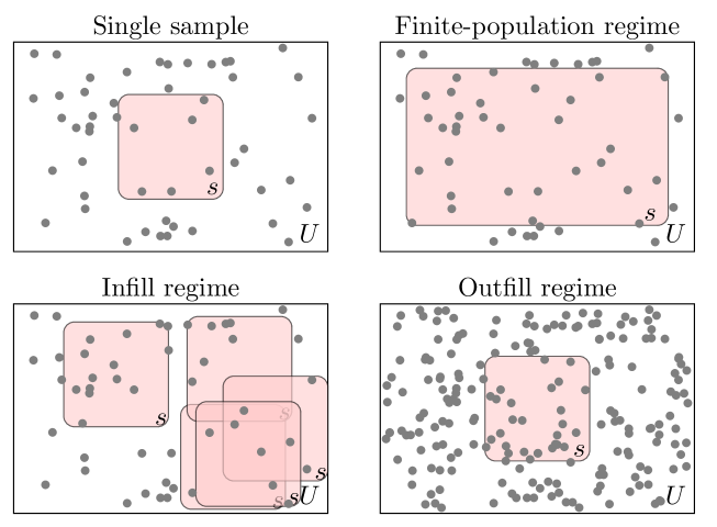
Figure 1: Illustration of different regimes for discrete sets. Units are indicated by circles. The sample $s$ “expands” to $U$ under the finite-population regime. Infinitely repeated samples of a fixed size are drawn from a fixed population under infill asymptotics. Under outfill, $s$ and $U$ grow simultaneously with $s$ approaching a fixed proportion of $U$.

The ratio $c_{i}$ can be greater than one when sampling is with replacement. The sample sizes mentioned above can be deterministic or random. In the latter case, all regimes can be defined in a similar way, e.g. $\mathbbm{E}|\bm{s}_{t}|/\mu(U_{t})\rightarrow c_{i}$. We are primarily interested in the outfill asymptotic regime with $k_{t}=1$ for all $t$. The binomial model as well as the multiplier and capture-recapture methods, described below, are special cases where $k_{t}$ may be greater than one. Figure 1 illustrates different regimes in general discrete settings.

2.3 Statistical properties of estimators

Let $\delta(\bm{s}_{t})$ be an estimator of $\mu(U_{t})$, defined for each $t$. We are interested in the statistical properties of $\delta(\bm{s}_{t})$ under the asymptotic regimes described above. An estimator is called unbiased if $\mathbbm{E}_{t}[\delta(\bm{s}_{t})]=\mu(U_{t})$ for all $t$, where $\mathbbm{E}_{t}(\cdot)$ denotes expectation with respect to $\mathbbm{P}_{t}$. Under an asymptotic regime $\{\bm{s}_{t},U_{t},\mathbbm{P}_{t}\}_{t=1}^{\infty}$, an estimator $\delta(\bm{s}_{t})$ is asymptotically unbiased if $\lim_{t\rightarrow\infty}\mathbbm{E}_{t}[\delta(\bm{s}_{t})]-\mu(U_{t})=0$. There may be some slightly biased estimators whose variance is smaller than that of every unbiased estimator. A common way to balance the trade-off between the bias and variance is to evaluate the mean squared error (MSE), defined as $MSE[\mu(U_{t}),\delta(\bm{s}_{t})]=\mathbbm{E}\left[(\delta(\bm{s}_{t})-\mu(U_{t}))^{2}\right]=(\mathbbm{E}[\delta(\bm{s}_{t})]-\mu(U_{t}))^{2}+\text{Var}[\delta(\bm{s}_{t})]$. The asymptotic MSE under a given regime is defined as $\lim_{t\rightarrow\infty}MSE(\mu(U_{t}),\delta(\bm{s}_{t}))$.

An estimator $\delta(\bm{s}_{t})$ that satisfies $\lim_{t\rightarrow\infty}\mathbbm{P}_{t}(|\delta(\bm{s}_{t})-\mu(U_{t})|>\varepsilon)=0$ for any $\varepsilon>0$ under a particular asymptotic regime $\{\bm{s}_{t},U_{t},\mathbbm{P}_{t}\}$ is called consistent for $\mu(U_{t})$. An estimator $\delta(\bm{s}_{t})$ is called MSE consistent for $\mu(U_{t})$ under a certain asymptotic regime if $MSE[\delta(\bm{s}_{t}),\mu(U_{t})]\rightarrow 0$ as $t\rightarrow\infty$ under that asymptotic setting. MSE consistency implies consistency. Under a particular asymptotic regime, we call a sequence of estimates $\delta(\bm{s}_{t})$ asymptotically normal with mean $\xi$, variance $\sigma^{2}/t^{r}$ and rate $t^{r}$ if the cumulative distribution function (CDF) of $t^{r}\left(\delta(\bm{s}_{t})-\xi\right)$ converges to the CDF of a $N(0,\sigma^{2})$ random variable, denoted by $t^{r}\left(\delta(\bm{s}_{t})-\xi\right)\xrightarrow{L}N(0,\sigma^{2})$.

3 Ordered sets: the German tank problem

Suppose each unit in the hidden set $i\in U$ has a distinct label $X_{i}\in\mathbbm{R}$, so that the labels give a natural ordering of the elements in $U$: we can define units $i<j$ if $X_{i}<X_{j}$. One common scenario for discrete $U$ is that the $X_{i}$’s are consecutive integers. Another common situation when $U$ is equivalent to an interval in $\mathbbm{R}$ is that $\cup_{i\in U}X_{i}$ equals that interval. An observation of samples from an ordered set $U$ consists of sampled units $s$ and their labels $\{x_{i}:\ i\in s\}$.

In 1943, the Economic Warfare Division of the American Embassy in London initiated a project to learn about the capacity of the German military using serial numbers found on German equipment [42, 78]. In a simple conceptualization of the problem, let $U=\{1,\ldots,N\}$ and consider sampling $n=|s|$ units without replacement from $U$ with probability $\mathbbm{P}(s)=1/{N\choose n}$. With $k_{t}$ i.i.d. repeated samples, an estimator $\delta(\bm{s})$ for $N$ is a functional of the observations, including the sample sizes and observed labels $X_{1,1},\ldots,X_{1,n},\ldots,X_{k_{t},1},\ldots,X_{k_{t},n}$. For example, to estimate the total number of participants in a marathon, if all $N$ participants are numbered by the consecutive integers $1,\ldots,N$, one could randomly record the first $n$ numbers they saw in the race, and estimate the total based on the observed numbers.

For the $k$th sample $X_{k,1},\ldots,X_{k,n}$, we let $X_{k(n)}$ be the $n$th order statistic in the sample. With one sample, the maximum likelihood estimator (MLE) for $N$ is $\widehat{N}_{MLE}=X_{(n)}$, which is negatively biased. Goodman [43] proposed an unbiased estimator

$$\widehat{N}_{G}=\frac{n+1}{n}X_{(n)}-1,$$ (1)

which is a uniformly minimum-variance unbiased estimator (UMVUE), with $\text{Var}(\widehat{N}_{G})=(N-n)(N+1)/n(n+2)$. An alternative estimator of $N$ takes into account the gap between $X_{(n)}$ and $N$, and adjusts for the bias with the average gap between order statistics [43]. The estimator

$$\widehat{N}_{2}=X_{(n)}+\frac{X_{(n)}-X_{(1)}}{n-1}-1,$$ (2)

is also unbiased, with $\text{Var}(\widehat{N}_{2})={n(N-n)(N+1)}/{(n-1)(n+1)(n+2)}$. The estimator $N_{2}$ can also be modified to estimate $N$ when the labels do not start with 1. In particular,

$$\widehat{N}_{3}=\frac{(n+1)\left(X_{(n)}-X_{(1)}\right)}{n-1}-1$$

is the UMVUE of $N$ when the initial label is unknown [43], with $\text{Var}(\widehat{N}_{3})=2(N-n)(N+1)/(n-1)(n+2)$.

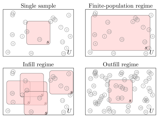
Figure 2: Illustration of a single sample, and the finite-population, infill, and outfill regimes for the German tank problem. Units with their labels are represented by circles with numbers inside.

When there is more than one sample, we take the MLE as the maximizer of the joint sampling probability $\mathbbm{P}_{t}(s_{1},\ldots,s_{k_{t}})$, which is $\max_{i\in[k_{t}]}X_{i(n)}$, the largest observed value across all $k_{t}$ samples. For estimators with closed forms like $\widehat{N}_{G},\widehat{N}_{2},\widehat{N}_{3}$, we derive $k_{t}$ estimates $\delta(s_{i}^{(t)}),\ i=1,\ldots,k_{t}$ based on each sample, and take their average as the estimator. In remaining sections, we average the estimators under infill by default, except for the models where infinite without-replacement sampling is feasible (e.g. Section 4.1). We consider the infill asymptotic regime where $n_{t}=n,N_{t}=N$ and $k_{t}\rightarrow\infty$, and the outfill regime where $n_{t},N_{t}\rightarrow\infty,k_{t}=1$ with $n_{t}/N_{t}\rightarrow c\in(0,1)$. Figure 2 illustrates different regimes for the German tank problem. We have the following asymptotic results:

Theorem 3.1.

Under the finite-population and infill regimes, $\widehat{N}_{MLE},\widehat{N}_{G},\widehat{N}_{2},\widehat{N}_{3}$ are consistent. Under the outfill regime, all estimators above are asymptotically unbiased with asymptotic MSE $O(1)$ and inconsistent. Whether the initial label is known or not does not change the rate of MSE of the UMVUE.

4 Bernoulli Trials

Consider a discrete hidden set $U$ consisting of $N$ unlabeled, indistinguishable units. A sample ${s}$ from $U$ arises by associating a binary indicator $Y_{i}\sim\text{Bernoulli}(p)$ to each $i\in U$, for fixed $0<p<1$, where different realizations of the $Y_{i}$’s can be generated in different draws. The probability $p$ may be known or unknown. A single sample consists of the subset of units with positive indicators, $s=\{i\in U:\ Y_{i}=1\}$. This is a frequently encountered situation in computer science, ecology, business, epidemiology, and many other fields [79, 80, 34, 33].

4.1 Binomial $N$ parameter

We first assume that $p$ is known. A single sample ${s}$ from $U$ gives a statistic $Q:=n=|s|=\sum_{i\in U}Y_{i}$ which has Binomial$(N,p)$ distribution. When there are $k$ independent samples, we assume they are generated by the same mechanism, so $\mathbbm{P}(Q_{1}=q_{1},\ldots,Q_{k}=q_{k})=\prod_{i=1}^{k}{N\choose q_{i}}p^{q_{i}}(1-p)^{N-q_{i}}$. The method of moments estimator (MME) $\widehat{N}_{MME}=\bar{Q}/p$ is an unbiased estimator of $N$. There are two versions of the MLE, derived from continuous and discrete likelihood equations respectively. The continuous MLE, $\widehat{N}_{MLE}^{\prime}$ is the solution of $\partial L/\partial N=0$ (take $Q_{(k)}$ if it is larger than the solution), and the discrete MLE $\widehat{N}_{MLE}$ is the largest $N$ such that $L(N)-L(N-1)\geq 0$.

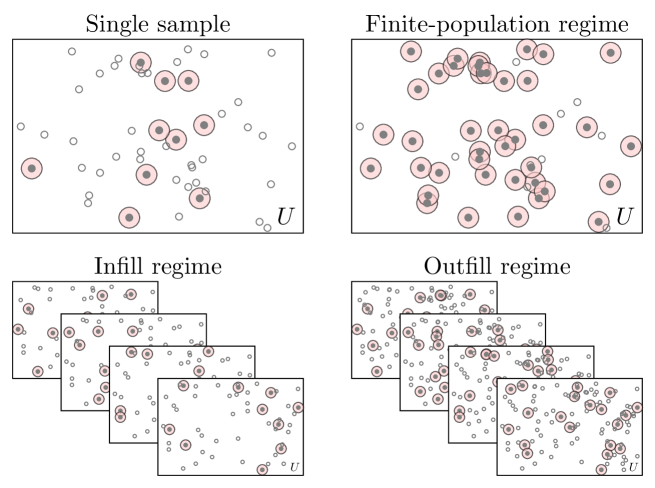
Figure 3: Illustration of the sampling mechanism for the binomial model, and the finite-population, infill and outfill asymptotic regimes. The solid points with red circles are units with indicator 1 (which are therefore in the sample), and the rest are unobserved.

The finite-population regime arises when $k=1$ and $p\rightarrow 1$, i.e. when all units are associated with indicator $1$ and observed in a single sample. We consider the infill asymptotic regime with $N_{t}=N$ and $k_{t}\rightarrow\infty$.The outfill regime is $k_{t},N_{t}\rightarrow\infty$ with $k_{t}/N_{t}\rightarrow c>0$. Figure 3 shows how the sampling mechanism varies under different regimes for the binomial $N$ model. The following theorem combines results in [81, 82] and states the consistency of estimates under the infill asymptotic regime, along with error rates under the outfill regime. In particular, the estimation error of $Q_{(k)}$ increases with $N$ under the outfill regime.

Theorem 4.1.

Under the finite-population regime, $\widehat{N}_{MME}$, $Q_{(k)}$ and $\widehat{N}_{MLE}$ are consistent. Under infill asymptotics, $\widehat{N}_{MLE},\widehat{N}_{MME}$, $Q_{(k)}$, and $\widehat{N}^{\prime}_{MLE}$ after rounding to the nearest integer, are consistent [81]. Under outfill asymptotics, $\widehat{N}_{MME}$ and $\widehat{N}^{\prime}_{MLE}$ are both asymptotically unbiased and normal with variance $O(1)$. The “relative error” of the discrete MLE, ${(\widehat{N}_{MLE}-N)}/{N^{\alpha}}\xrightarrow{P}0$ for any $\alpha>1/2$. The “relative error” of $Q_{(k)}$ with $\alpha=1$ goes to $p-1$ in probability.

When $p$ is unknown, the situation does not improve: negative or unstable estimates may occur, and Bayesian approaches are usually adopted to avoid these issues. Blumenthal and Dahiya [81] adopted a conjugate prior Beta$(a,b)$ for $p$ and an improper uniform prior $p(N)\propto 1$ for $N$; the posterior is proper if and only if $a>1$ [83]. Blumenthal and Dahiya [81] showed that the posterior mode $\widehat{N}_{m}$ is consistent under infill asymptotics, and satisfies

$$\frac{\sqrt{n}}{N}\left(\widehat{N}_{m}-N\right)\xrightarrow{L}N\left(0,\frac{2(1-p)^{2}}{p^{2}}\right)$$

under the outfill regime. In particular, the MSE rate is slower compared to $O(1)$ as in Theorem 4.1 when $p$ is known.

A special case of the Binomial scenario arises for zero-truncated counts. For example, a registry may record the number of times each unit has been observed, but zero counts are not recorded. Distributional assumptions can be used to estimate the proportion of unobserved zero counts, leading to estimates of the set size. Zero-truncated counting models have been used to estimate size of hard-to-reach populations, including drug users [84, 85], undocumented immigrants [86, 87], criminal population [88, 89], the number of infected households in an epidemic [90], and species richness in ecology [91, 92]. To illustrate, associate to each unit $i\in U$ a realization of the attribute $Y_{i}\sim\text{Poisson}(\lambda)$. A sample from $U$ is $s=\{i\in U:\ Y_{i}>0\}$ and an observation on $s$ is $\{Y_{i}:\ i\in s\}$, the set of all positive counts. For one sample, the sampling mechanism is given by $\mathbbm{P}(y_{1},\ldots,y_{|s|}|s)=\prod_{i\in s}\lambda^{y_{i}}/(e^{\lambda}-1)y_{i}!$. Estimating $\lambda$ under this model reveals the proportion of zero counts, $p=1-e^{-\lambda}$, and estimation of $N$ proceeds as in the Binomial$(N,p)$ case outlined above. The asymptotic results in Theorem 4.1 follow.

4.2 Waiting times

Sometimes the state of a hidden unit may change, thereby making it known to an observer. For example, terrorist plots may change state from “hidden” to “executed”, making them observable by intelligence agents [45]. The temporal pattern of such state changes may give insight into the number of hidden units. Properties of waiting times to an event have been exploited to estimate the number of units in studies of terrorism, crime, and estimation of epidemiological risk population sizes [45, 93, 94, 95].

Suppose $U$ is a set of $N$ hidden units in existence at time 0, each of which is at risk of “failure” at some future time. To each $i\in U$, associate a failure time $T_{i}\sim\text{Exponential}(\lambda)$, and suppose failure times are observed up to some finite observation time $T>0$. A sample is the set of units that have failed by the end of study, $s=\{i\in U:\ T_{i}<T\}$ with $|s|=n$, and an observation on $s$ is $\{T_{i}:i\in s\}$. With repeated sampling, a new observation is independent of all previous observations, taken after all units are set to be “at risk” over again. We consider the finite-population regime in which $T\rightarrow\infty$ so that all failures are observed, the infill regime in which $T$ and $N$ are fixed with the number of repeated observations $k_{t}\rightarrow\infty$, and the outfill regime in which $T_{t},N_{t}\rightarrow\infty$ with $T_{t}/N_{t}\rightarrow c>0$. For example, if $U$ is the set of hidden terrorist plots [e.g. 45, 46], the finite-population regime keeps $|U|=N$ constant, while letting the maximum observation time $T\to\infty$, so that eventually every plot in $U$ is executed and thereby revealed to the observer. The infill regime consists of keeping $N$ and $T$ constant, while obtaining (hypothetical) repeated realizations of the same $N$ plots over $[0,T]$. The outfill regime lets both the observation time $T$ and number of plots $N$ go to infinity together, so that more plots are added, while the observation time increases. Figure 4 illustrates each regime under the waiting time model.

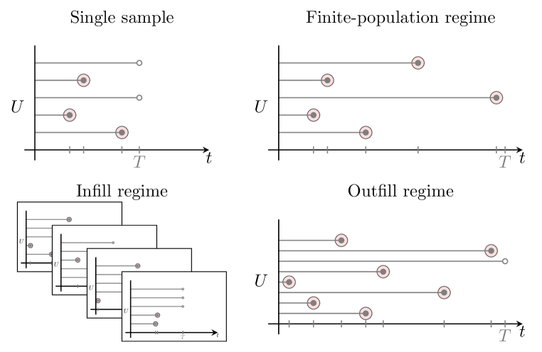
Figure 4: Illustration of the waiting time model. The observed event times are subject to right censoring at $t=T$, that is, events that occur before $T$ are observed. Solid dots with red shades indicate observed event times. The finite-population regime is that $T\rightarrow\infty$ so that all events are observed. Infill asymptotics amounts to generating different realizations of the failure times. Under the outfill regime, $T$ and the total number of units $N$ both increase toward infinity.

Let $\Delta_{i}:=T_{i}-T_{i-1}$ be the waiting time between the $(i-1)$th and $i$th failure. The sampling mechanism is given by

$$\mathbbm{P}(t_{1},\ldots,t_{n}|N,\lambda)=\lambda^{n}\cdot\prod_{i=1}^{n}(N-i+1)\cdot\exp\left[-\lambda\sum_{i=1}^{n}(N-i+1)\Delta_{i}\right]\cdot\exp[-\lambda(N-n)(T-t_{n})],$$

which gives rise to the likelihood $L(t_{1},\ldots,t_{n};N)$. Alternatively, if we ignore the timing of events, the observed number of events can be characterized by a binomial model $\mathbbm{P}(n|N,\lambda)={N\choose n}(1-e^{-\lambda T})^{n}e^{-\lambda T(N-n)}$, which yields $L_{2}(n;N)$. Maximizing $L$ and $L_{2}$ lead to two estimates, $\widehat{N}_{MLE}$ and $\widehat{N}^{\prime}_{MLE}$ of $N$. It is easy to verify that $\partial\log L/\partial N=\partial\log L_{2}/\partial N$, so $\widehat{N}_{MLE}$ and $\widehat{N}^{\prime}_{MLE}$ are identical. The timing of events does not contain more information about $N$ than the total number of events. The asymptotic behavior of $\widehat{N}_{MLE}$ follows from the discussion in Section 4.1: when $\lambda$ is known, $\widehat{N}_{MLE}$ is consistent under finite-population and infill regimes. Under the outfill regime, it is unbiased and asymptotically normal with variance $O(1)$.

4.3 The network scale-up method

Estimating the number of vertices in a hidden network or graph is an important problem in sociology, epidemiology, computer science, and intelligence applications [5, 48, 52, 54, 55, 96, 97]. A subgraph of a larger graph may contain information about the size of the larger graph [55, 98, 99]. The network scale-up method (NSUM) [5] provides an estimate for the size of a hidden population by making use of network information from a sub-sample of individuals.

Consider a graph $G_{V}=(V,E)$, where $V$ is a set of $M$ units and $\{i,j\}\in E$ means that $i,j\in V$ are connected. $V$ is called the total population, and a subset $U\subseteq V$ of size $N$ is the hidden population. Assume $G_{V}$ is simple, and has no parallel edges or self-loops. The network of $U$ is $G_{U}=(U,E_{U})$, where $E_{U}=\{\{i,j\}:i\in U,j\in U,\{i,j\}\in E\}$. We call $V\setminus U$ the general population. A sample from a subset of $V$, along with network degrees of the sampled units within and outside of that subset provides information for learning about the size of $U$. Suppose the total population network $G_{V}$ is generated from the Erdős-Rényi random graph model [100] in which each pair of distinct vertices is connected independently by an edge with probability $\Pr(\{i,j\}\in E)=\pi$. The likelihood of a random graph $G_{V}=(V,E)$ from the Erdős-Rényi model with $|V|=N$ and connection probability $\pi$ is

$$\Pr(G_{V})=\pi^{|E|}(1-\pi)^{\binom{N}{2}-|E|}$$

where $|E|$ is the number of edges and $\binom{N}{2}$ is the number of unordered distinct pairs of vertices. Two common sampling scenarios – sampling from $V\setminus U$ and directly from $U$ – are illustrated in Figure 5.

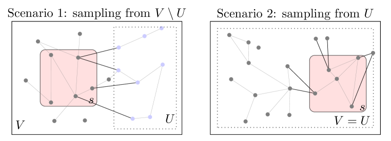
Figure 5: Illustration of the two common scenarios for the network scale-up method. In scenario 1, $U\subset V$ and we observe a randomly chosen subset $s$ of $V\setminus U$ and number of edges from each unit in $s$ to $U$ (thick lines) and to $V\setminus U$ (thin lines) respectively. In scenario 2, $U=V$ and we observe the induced subgraph (edges represented by thin lines) from a randomly chosen subset $s$ of $U$ as well as the pendant edges (thick lines) between $s$ and $U\setminus s$.

4.3.1 Sampling from the general population

We consider sampling uniformly at random from the general population $V\setminus U$ with a fixed sample size $|s|=n$. The sampling mechanism is $\mathbbm{P}(s\mid|s|=n)=\binom{M-N}{n}^{-1}$. For a sample $s\in V$, we observe network degrees $d_{i}^{V}:=\sum_{j\in V}\mathds{1}\{E_{ij}=1\}$ and $d_{i}^{U}:=\sum_{j\in U}\mathds{1}\{E_{ij}=1\}$ for each $i\in s$. As an empirical example, suppose we wish to estimate the number of people who died in an earthquake [e.g. 98]. We cannot survey the dead (members of $U$) but we can survey living people ($V\setminus U$) to determine how many people they know ($d_{i}^{V}$), and how many they know who died as a result of the earthquake ($d_{i}^{U}$).

Under the Erdős-Rényi model, $\mathbbm{E}d_{i}^{V}=(M-1)\pi\approx M\pi$ and $\mathbbm{E}d_{i}^{U}=N\pi,\ \forall i\in V\setminus U$. Taking the ratio and canceling out $\pi$ yields the MME

$$\widehat{N}_{NS}=M\cdot\frac{\sum_{i=1}^{n}d_{i}^{U}}{\sum_{i=1}^{n}d_{i}^{V}}.$$ (3)

Conditional on $d_{i}^{V}$, $d_{i}^{U}$ follows hypergeometric distribution for each $i$. The same estimator can also be derived under a different model assumption. Killworth et al. [5] considered a model where $d_{i}^{U}$ is Binomial$(d_{i}^{V},N/M)$ given $d_{i}^{V}$, and (3) is then the MLE under this binomial model, which is unbiased with variance $(M-N)N/\sum_{i}d_{i}^{V}$.

We consider the finite-population regime in which $n\rightarrow(M-N)$, i.e. $s\rightarrow V\setminus U$. Under the infill regime, $M,N,n$ are fixed and the number $k_{t}$ of repeated samples $s\subseteq V\setminus U$ goes to infinity. The outfill regime is that $M_{t},N_{t},n_{t}\rightarrow\infty$ such that $N_{t}/M_{t}\rightarrow c_{1}\in(0,1)$, $n_{t}/(M_{t}-N_{t})\rightarrow c_{2}\in(0,1)$, and $k_{t}=1$.

Sometimes an intermediate step in deriving $\widehat{N}_{NS}$ is the estimation of personal network sizes $d_{i}^{V}$. If unbiased estimates $\hat{d_{i}^{V}}$ are plugged in, $\widehat{N}_{NS}$ would have a positive bias by Jensen’s inequality since $1/x$ is a convex function. Let us assume for now that the $d_{i}^{V}$’s are observed true values. Theorem 4.2 states the asymptotic properties of $\widehat{N}_{NS}$ under the Erdős-Rényi assumption.

Theorem 4.2.

$\widehat{N}_{NS}$ has a positive bias $N/(M-1)$. It is not necessarily consistent under the finite-population regime, and converges to a positively biased quantity under infill. It is asymptotically normal with bias $c_{1}$ and variance $O(1)$ under the outfill regime.

4.3.2 Sampling from the hidden population

When possible, a random sample from the hidden population $U$ can also lead to a valid estimate. Consider a random sample $s\subseteq U$ where $G_{U}$ follows the Erdős-Rényi model with edge probability $\pi$. We observe the nodes $i\in s$, as well as network degrees $d_{i}^{s}:=\sum_{j\in s}\mathds{1}\{E_{ij}=1\}$ and $d_{i}^{U}:=\sum_{j\in U}\mathds{1}\{E_{ij}=1\}$, for each individual $i\in s$. Then, $\mathbbm{E}\left(\sum_{i\in s}d_{i}^{U}\right)=2{n\choose 2}\pi$ and $\mathbbm{E}\left(\sum_{i\in s}d_{i}^{s}\right)=\pi n(N-1)$. Canceling out $\pi$ yields the MME, which is often simplified to

$$\widehat{N}=\frac{n\sum_{i=1}^{n}d_{i}^{U}}{\sum_{i=1}^{n}d_{i}^{s}}.$$ (4)

Chen et al. [101] investigated the behavior of $\widehat{N}$ with finite-sample as well as with large $n$, but did not specify the relationship between $N$ and $n$ under the asymptotic setting. In our setting, the finite-population regime is $n\rightarrow N$ with $N$ fixed. The infill regime is that $n,N$ are fixed and the sampling procedure is infinitely repeated. The outfill asymptotic regime is that $n_{t},N_{t}\rightarrow\infty$ with $n_{t}/N_{t}\rightarrow c\in(0,1)$. Then we have the following theorem for the asymptotic properties of $\widehat{N}$.

Theorem 4.3.

Under the finite-population regime, $\widehat{N}$ converges to $N$. Under infill asymptotics, $\widehat{N}$ is always positively biased conditioning on $|E_{s}|>0$ [101], and is hence inconsistent. Under outfill asymptotics, $\widehat{N}$ is asymptotically normal with bias $(1-c)/c$ and variance $O(1)$.

4.4 Estimating a total with unequal sampling probabilities

A generalization of binomial models allows for heterogeneity in the inclusion, or “success” probabilities $p$, that is, when the sampling is not uniformly at random. Horvitz and Thompson [50] proposed unbiased estimators for population means and totals under the setting of sampling without replacement from finite population, where the selection probabilities can be unequal. The Horvitz-Thompson (HT) estimator for the population total is $\widehat{N}=\sum_{i\in s}{1}/{p_{i}}$, where $p_{i}=\mathbbm{E}(\mathds{1}\{i\in s\})$ is the probability that unit $i\in U$ is sampled in $s$. The estimator $\widehat{N}$ is unbiased for the total population size $N$. This estimator and its variants have been applied to the estimation of animal abundance [102] and other fields. We consider a deterministic sample size $n$. Then the variance of $\widehat{N}$ is [50]

$$\text{Var}(\widehat{N})=-\frac{1}{2}\sum_{i=1}^{N}\sum_{j=1}^{N}(p_{ij}-p_{i}p_{j})\left(\frac{1}{p_{i}}-\frac{1}{p_{j}}\right)^{2},$$ (5)

where $p_{ij}$ is the joint probability that units $i$ and $j$ are both in the sampled set $s$, and $p_{ii}=p_{i}$. The finite-population regime amounts to letting $p_{i}\rightarrow 1$ for any $i$. Under the infill regime, $p_{i},p_{ij},N$ are fixed and the number of repeated samples $k_{t}\rightarrow\infty$. Under the outfill regime, $N$ and $n$ both increase to infinity such that $n/N\rightarrow c\in(0,1)$. Figure 6 shows the non-uniform sampling mechanism under each regime.

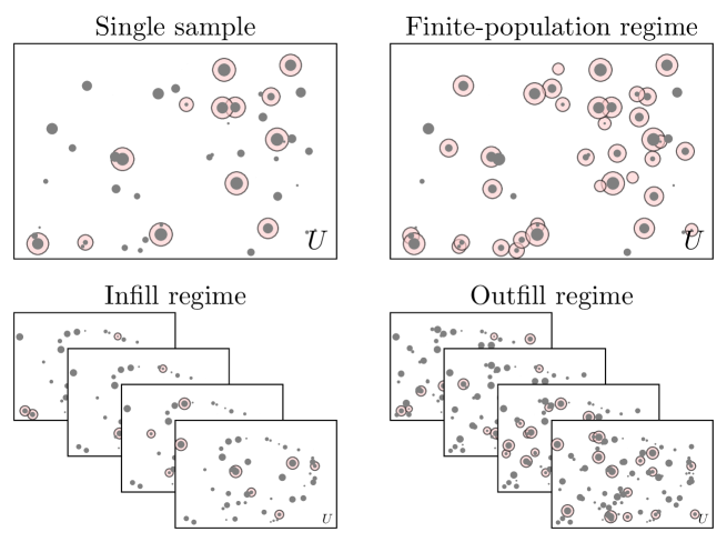
Figure 6: Illustration of the single sample, finite-population, infill and outfill regimes for the general HT estimator. The probability of being sampled for each point here is visualized as its size.

Specifically, we consider the following setting to illustrate the asymptotic behavior of the HT estimator. Suppose $U$ consists of $H$ clusters, where the $h$th cluster has $N_{h}$ units. We assume that $H$ is known in advance, while $N_{h}$ is observed only if a unit from cluster $h$ is sampled. In each sample, a total of $n$ units are sampled from $U$ by the following procedure: first a cluster $h$ is drawn uniformly at random each with probability $1/H$. Then one unit is drawn from the $N_{h}$ units in that cluster, also uniformly at random, without replacement. We assume that $\min_{h\in[H]}N_{h}>n$. An observation on sample $s$ consists of the units in $s$, their cluster membership, and the sizes of clusters that they belong to.

When there are repeated observations, we assume they follow the same design and are mutually independent. In this setting, the outfill regime is defined such that each cluster in the original population is replicated and appears $t$ times in $U_{t}$. The cluster sizes are fixed at $N_{h}^{(t)}=N_{h}$ and the number of clusters increases as $H_{t}=tH$. $N=\sum_{h=1}^{H}$ is fixed and the estimand is $N_{t}=Nt$. The sample size satisfies $n_{t}/N_{t}\rightarrow c\in(0,1)$. We then have the following theorem about the consistency of $\widehat{N}$ under each regime. In particular, the variance of $\widehat{N}$ grows with $N$ under the outfill regime.

Theorem 4.4.

$\widehat{N}$ is consistent under the finite-population regime, and MSE consistent under infill asymptotics. $\widehat{N}$ is unbiased and asymptotically normal with variance $O(N)$ under the outfill regime.

5 Other unordered sets

5.1 Capture-recapture experiments

Capture-recapture (CRC) refers to a broad class of methods to estimate the size of hidden populations for which random sampling is possible [35, 58, 57, 103, 104, 105]. Estimation of the population size is based on the overlap between two or more random samples [31, 32, 8, 15]. While a wide variety of CRC estimators have been developed [106, 107, 103, 104, 108], we focus here on the two- and $k$-sample CRC estimators with homogeneity within a closed population.

5.1.1 Two-sample estimation

We first consider the common case of two-sample CRC. Let $U$ be a hidden finite set of size $N$, where each unit $i\in U$ has binary attributes $(X^{1}_{i},X^{2}_{i})$, which are all $(0,0)$ in the beginning. We draw a sample $s_{1}\subseteq U$ with size $n_{1}$ from $U$, and set $X^{1}_{i}=1$ for all $i\in s_{1}$. Then a second sample $s_{2}$ with size $n_{2}$ is drawn, independent from $s_{1}$ and uniformly at random, and we set $X^{2}_{i}=1$ for all $i\in s_{2}$. We observe $(X^{1}_{i},X^{2}_{i})_{i\in s_{1}\cup s_{2}}$, and let $m=\sum_{i\in U}\mathds{1}\{(X^{1}_{i},X^{2}_{i})=(1,1)\}$. In ecology, to estimate the abundance of an animal species, researchers could first capture $n_{1}$ animals from that species, mark them and then release them. After the captured animals have mixed well with the remaining ones, researchers could capture $n_{2}$ animals again, uniformly at random, and record the number $m$ of animals captured in the first step. Then $m$ follows a hypergeometric distribution conditioning on $N,n_{1}$ and $n_{2}$, i.e. the mechanism of generating the observations can be defined as $\mathbbm{P}(m|s_{1},s_{2})={n_{1}\choose m}{N-n_{1}\choose n_{2}-m}/{N\choose n_{2}}$. The MME, $\widehat{N}_{L}={n_{1}n_{2}}/{m}$, is also known as the Lincoln-Petersen estimator [109, 110].

We consider the finite-population regime with $n_{2}\rightarrow N$. The infill regime is that $N,n_{1},n_{2}$ are fixed and repeated sample pairs $\{s_{1}^{(t)},s_{2}^{(t)}\}$ are drawn with $t\rightarrow\infty$. The outfill regime is given by $N^{(t)},n_{1}^{(t)},n_{2}^{(t)}\rightarrow\infty$ with $n_{i}^{(t)}/N^{(t)}\rightarrow c_{i}\in(0,1)$ for $i=1,2$.

Previous results exist on the bounds or estimates of biases and variances. These were implicitly based on asymptotic approximations: Chapman [56] showed a lower bound for the bias

$$\mathbbm{E}\left(\widehat{N}_{L}\right)-N\geq N\left[\frac{N}{n_{1}n_{2}}+2\left(\frac{N}{n_{1}n_{2}}\right)^{2}\right]$$

under outfill, and bounded the variance as

$${\text{Var}}(\widehat{N}_{L})>N^{2}\left[\left(\frac{N}{n_{1}n_{2}}\right)+\left(\frac{N}{n_{1}n_{2}}\right)^{2}\right]$$

under asymptotic approximation that was satisfied by the outfill regime. Though these no longer hold under finite-sample setting, calculations in [56] showed that $\widehat{N}_{L}$ has a considerable bias under a range of settings. A less biased estimator

$$\widehat{N}_{C}=\frac{(n_{1}+1)(n_{2}+1)}{m+1}-1,$$ (6)

was proposed [56], with bias

$$\mathbbm{E}(\widehat{N}_{C})-N=-\frac{(N-n_{1})!(N-n_{2})!}{N!(N-n_{1}-n_{2}-1)!}$$ (7)

for any $n_{1},n_{2},N$, and variance

$$\text{Var}(\widehat{N}_{C})\sim N^{2}\left[\frac{N}{n_{1}n_{2}}+2\left(\frac{N}{n_{1}n_{2}}\right)^{2}+6\left(\frac{N}{n_{1}n_{2}}\right)^{3}\right]$$ (8)

under outfill [56], where $\sim$ means the difference between two quantities decay to 0. We have the following asymptotic result of $\widehat{N}_{L}$ and $\widehat{N}_{C}$. Specifically, both estimators have infinitely increasing estimation error under the outfill asymptotic setting.

Theorem 5.1.

Under the finite-population regime, $\widehat{N}_{L}$ and $\widehat{N}_{C}$ are consistent. Under infill asymptotics, $\widehat{N}_{L}$ is positively biased and has MSE $O(1)$ for at least a range of values of $n_{1},n_{2},N$. $\widehat{N}_{C}$ is negatively biased, but the bias is within 1 if $n_{1}+n_{2}+1<N/2$ and $n_{1}n_{2}/N>\log N$ [56]. Under the outfill regime, $\widehat{N}_{L}$ has bias at least $O(1)$ and variance at least $O(N)$. $\widehat{N}_{C}$ is asymptotically unbiased with variance $O(N)$. Furthermore, $\widehat{N}_{C}$ and $\widehat{N}_{L}$ are inconsistent with $\mathbbm{P}(|\widehat{N}_{C}-N|<\varepsilon)\rightarrow 0$ and $\mathbbm{P}(|\widehat{N}_{L}-N|<\varepsilon)\rightarrow 0$ for some $\varepsilon>0$ when $n_{1}=c_{1}N,n_{2}=c_{2}N$.

Further, Chapman [56] showed that no estimator can be unbiased for all possible values of $N,n_{1}$ and $n_{2}$.

A similar but slightly different sampling mechanism gives rise to the multiplier method, also called the method of benchmark multiplier (MBM). In practice, researchers may know the number of hidden units with a certain trait. The overall prevalence of that trait in the hidden population, if available from estimation, would provide an estimate for the size of the hidden population. Often the prevalence is estimated through expert opinion, historical data, or from a separate sample [111, 112, 23].

We consider the last approach. The idea of MBM can be expressed with a sampling mechanism similar to CRC, except that the first sample $s_{1}$ is fixed under infill asymptotics. That is, the known sub-population of hidden units with a certain trait is fixed. The size $n_{1}$ of $s_{1}$ is called the benchmark. The proportion $m/n_{2}$ gives the multiplier, which is an estimate of the prevalence $p$. Again, $m$ follows a hypergeometric distribution, so the MME for $N$ is $\widehat{N}_{MBM}=n_{1}n_{2}/{m}$, which is often called the multiplier estimator. $\widehat{N}_{MBM}$ takes the same form as the Lincoln-Petersen CRC estimator. Asymptotic behaviors of $\widehat{N}_{MBM}$, as summarized in Theorem 5.2, are essentially the same as that of $\widehat{N}_{L}$ for CRC.

Theorem 5.2.

$\widehat{N}_{MBM}$ is consistent under the finite-population regime. Under infill asymptotics, $\widehat{N}_{MBM}$ is inconsistent with MSE $O(1)$. Under the outfill regime, when $n_{1}=c_{1}N$, and $n_{2}=c_{2}N$, $\widehat{N}_{MBM}$ is inconsistent with MSE at least $O(N)$. $\mathbbm{P}(|\widehat{N}_{MBM}-N|<\varepsilon)\rightarrow 0$ for some $\varepsilon>0$.

5.1.2 $\bm{k}$-sample estimation

We now consider the generalized setting of $k$ samples. In this scenario, we draw $k$ samples $s_{1},\ldots,s_{k}\subseteq U$ with deterministic sizes $n_{1},\ldots,n_{k}$ respectively. We assume the probability $p_{j}:=n_{j}/N$ of being observed in the $j$th sample is the same for each unit for $j=1,\ldots,k$. In each sample (say $s_{j}$), we give the observed units a label that is different for different $j$’s, and record the capture history $\mathcal{H}_{j,i}=(I_{1}^{(i)},\ldots,I_{j}^{(i)})$ of each unit $i\in s_{j}$, where $I_{l}=1$ if $i\in s_{l}$ and 0 otherwise $(l\leq j)$. Then an observation on a sequence of samples $\bm{s}=\{s_{1},\ldots,s_{k}\}$ is a $2^{k}$ contingency table $T=\{T_{I_{1}\ldots I_{k}}\}_{I_{1},\ldots,I_{k}\in\{0,1\}^{k}}$ [58], where the entry corresponding to $I_{1},\ldots,I_{k}$ is $\sum_{i\in U}\mathbbm{1}(I_{1}^{(i)}=I_{1},\ldots,I_{k}^{(i)}=I_{k})$, the number of units with capture history $\mathcal{H}_{k}=(I_{1},\ldots,I_{k})$. Let $r$ be the sum of known entries in the contingency table – only the entry $T_{0\ldots 0}$ is unobserved. In plain words, following the animal abundance example, researchers could instead draw $k$ random samples. In the first $k-1$ samples, animals that are captured will be given a mark that is unique for each sample. The contingency table summarizes the capture history for all observed animals – how many animal(s) are observed in, or absent from, which sample(s). From the contingency table we have $m_{i}$, the number of already marked individuals in $s_{i}$, and $M_{i}$, the total number of marked individuals in $U$ before $s_{i}$ is drawn. The sampling scheme then follows a generalized hypergeometric distribution:

$$\mathbbm{P}(T|s_{1},\ldots,s_{k})=\frac{N!}{\prod_{I_{1},\ldots,I_{k}\in\{0,1\}^{k}}T_{I_{1}\ldots I_{k}}!(N-r)!}\prod_{i=1}^{k}{N\choose{n_{i}}}^{-1}.$$ (9)

Maximizing the likelihood (9) gives the MLE of $N$ as the solution of

$$\left(1-\frac{r}{N}\right)=\prod_{i=1}^{k}\left(1-\frac{n_{i}}{N}\right),$$ (10)

which is unique, finite and greater than $r$ if $s_{1}\cap\ldots\cap s_{k}$ is non-empty and $|s_{i}|<r$ for all $i\leq k$ [57]. We restrict our interest to this case only. Setting $k=2$ recovers the Lincoln-Petersen estimator $\widehat{N}_{L}$. Since finite-population and infill regimes for the two- and $k$-sample cases are similar in essence, we mainly discuss outfill asymptotics in this setting: for any finite $k$, we have $N,n_{1},\ldots,n_{k}\rightarrow\infty$ with $n_{i}/N_{i}\rightarrow c_{i}\in(0,1)$ for $i=1,\ldots,k$, and $k_{t}$ may be finite or going to infinity. We assume the $c_{i}$’s are bounded away from 0 and 1. Under outfill asymptotics with finite $k$, following from the delta method, the bias of the MLE is approximated by [57]

$$\mathbbm{E}\left(\widehat{N}_{MLE}\right)-N\sim\frac{\left[\frac{k-1}{N}-\sum\left(\frac{1}{N-n_{i}}\right)\right]^{2}+\left[\frac{k-1}{N^{2}}-\sum\left(\frac{1}{N-n_{i}}\right)^{2}\right]}{2\left[\frac{1}{N-\mathbbm{E}[r]}+\frac{k-1}{N}-\sum\left(\frac{1}{N-n_{i}}\right)\right]^{2}},$$

which is $O(1)$, and the asymptotic variance is $O(N)$, approximated by [57]

$${\text{Var}}(\widehat{N}_{MLE})\sim\left[\frac{1}{N-\mathbbm{E}[r]}+\frac{k-1}{N}-\sum_{i=1}^{k}\left(\frac{1}{N-n_{i}}\right)\right]^{-1}.$$

Under outfill asymptotics with infinite sampling repetitions, we assume $\inf_{i\in[k]}p_{i}>0$. Then the magnitude of bias is bounded above by $N-\mathbbm{E}[r]$, and hence by $N\prod_{i=1}^{k}(1-p_{i})$. The variance is $O(N\prod_{i=1}^{k}(1-p_{i}))$. Therefore, as long as $k$ is increasing such that $N\prod_{i=1}^{k}(1-p_{i})\rightarrow 0$, $\widehat{N}_{MLE}$ will be MSE consistent for $N$.

6 Discussion

Several features determine researchers’ ability to learn about the size of a hidden set. First, the structure of the set – labeled units, ordering of the labels, or relational (network/graph) information – can permit researchers to learn about the number of remaining units when a subset is observed. Second, a feasible probabilistic query mechanism – random sampling, or observation conditional on a unit trait or attribute – must be available. Third, a statistical estimator that enjoys desirable statistical properties must be chosen. Some of these features may be under the control of researchers, while others may be intrinsic to the problem. Table 1 summarizes the models that have been discussed in this paper, as well as consistency results of estimators in each model.

Problem	Trait	Sample	Estimator	Consistency
German tank	Consecutive integers	Uniform random draw from $U$	$\widehat{N}_{\text{MLE}},\widehat{N}_{G},\widehat{N}_{2},\widehat{N}_{3}$	Infill: consistent Outfill: MSE $O(1)$
Binomial $N$	$Y_{i}\sim$Bernoulli($p$)	$\{i\in U:Y_{i}=1\}$	$\widehat{N}_{\text{MLE}},\widehat{N}_{\text{MME}}$, $Q_{(k)},\widehat{N}^{\prime}_{\text{MLE}}$	Infill: consistent Outfill: $\widehat{N}_{\text{MME}},\widehat{N}^{\prime}_{\text{MLE}}$ have MSE $O(1)$1
Waiting times	$T_{i}\sim$Exponential$(\lambda)$	$\{i\in U:T_{i}<T\}$	Equivalent to Binomial $N$
NSUM	Network degree $d_{i}^{U},d_{i}^{V}$	Uniform random draw from $V\setminus U$	$\widehat{N}_{NS}=M\frac{\sum d_{i}^{U}}{\sum d_{i}^{V}}$	Infill: inconsistent Outfill: MSE $O(1)$
	Network degree $d_{i}^{s},d_{i}^{U}$	Uniform random draw from $U$	$\widehat{N}=n\frac{\sum d_{i}^{U}}{\sum d_{i}^{s}}$	Infill: inconsistent2 Outfill: MSE $O(1)$
HT	Cluster membership	Uniform random draw from each sampled cluster	$\widehat{N}=\sum 1/p_{i}$	Infill: consistent Outfill: MSE $O(N)$
$k$-sample CRC	Capture history	$\mathbbm{P}(i\in s_{j})=n_{j}/N,\forall i$	$\widehat{N}_{L},\widehat{N}_{C},\widehat{N}_{MLE}$	Infill: inconsistent Outfill $k=2$: MSE $O(N)$ Outfill $k\rightarrow\infty$: $\widehat{N}_{MLE}$ consistent3
MBM	Similar to two-sample CRC

Table 1: Summary of models, estimators, and asymptotic results for estimating the size of a hidden set. Notes: 1. the error rate of $\widehat{N}_{MLE}$ and $Q_{(k)}$ are given in Section 4.1 in terms of relative error; 2. conditioning on $|E_{s}|>0$; 3. if $N\prod_{i=1}^{k}(1-p_{i})\rightarrow 0$.

How should empirical researchers evaluate the statistical properties of estimators, design a study or choose a sample size? Many of these tasks are based on asymptotic arguments, and statistical claims about the large-sample performance of hidden set size estimators depend on specification of an appropriate asymptotic (or even non-asymptotic) regime. It is crucial to identify how the sample size increases, especially in relation to the target population, when asymptotic approximation or comparison is involved in population size estimation tasks. When designing a study, this may include determining the minimum sample size that leads to a desired precision [113, 114], or selecting an “optimal” sampling strategy (e.g. one-time larger sample versus multi-time repeated smaller samples). In data analysis, this may include establishing valid approximation to biases and variances or comparing the efficiency of different statistical approaches [113, 115, 116, 117]. If the vast majority of the target population can be observed in one-step sampling, consistency under the trivial finite-population regime may be a goal when developing estimators. If the total population is fixed, and arbitrarily repeated i.i.d. samples can be obtained, then consistency under infill may justify the use of a statistical approach. If instead only one-time or finite-time sampling is permitted, in which the sample size is believed to reflect a proportion of the potentially large population, performance of estimators under outfill may be of more interest. We have shown that different asymptotic regimes can lead to dramatically different statistical properties. Some seemingly sensible estimators are inconsistent with different rates of MSE, and asymptotic claims for population size estimators under one regime may be of limited value for analyzing the general situation.

In this review, we have focused on technical claims about the asymptotic properties of estimators, and have not discussed considerations for practical data collection. For example, the waiting time model does not accommodate censoring or truncation of observations, but could be easily extended to do so. Respondent recall bias in the network scale-up method may make the reported network degrees noisy estimates of the truth. The Horvitz-Thompson estimator relies on knowledge about marginal inclusion probabilities of each sampled individual, which may not be readily available when the size of the population is unknown. While improved data collection strategies may not be able to mitigate poor asymptotic properties – like inconsistency – under a particular regime, better data may be able to reduce variance in finite samples.

While we have discussed many of the most popular settings and methods for estimating the size of a hidden set, there are several other settings we have not covered. Respondent-driven sampling (RDS), snowball sampling and link-tracing sampling generate samples from hidden networks, and modeling the stochastic process underlying such sampling mechanism can be used to estimate hidden population sizes [2, 95, 118, 119]. There is a large literature on CRC beyond what we have covered here. For example, there are approaches for CRC with an open population, with immigration, emigration, birth, and death [106, 107] or with heterogeneity in capture probabilities [103, 104]. CRC is also possible using data from network sampling designs [108]. We have also not discussed species number estimation [120], “count distinct” and streaming estimation problems [121, 122, 123], and genetic methods for population size estimation [124, 125]. In addition, we have not addressed the issue of entity resolution, or record de-duplication [47]. The results presented in this paper suggest that researchers employing methods for estimating the size of a hidden set should evaluate the performance of estimators under deliberately specified asymptotic assumptions.

Appendix A Asymptotic normality and consistency

We first introduce a simple lemma that helps to prove consistency or inconsistency based on asymptotic normality.

Lemma 1 (Asymptotic normality and consistency).

Suppose $a_{t}\left(X_{t}-\nu_{t}\right)\xrightarrow{L}N(0,\sigma^{2})$ for a finite $\sigma$. Then $X_{t}-\nu_{t}\xrightarrow{P}0$ if and only if $a_{t}\rightarrow\infty$ as $t\rightarrow\infty$.

Proof.

Assume $a_{t}\rightarrow\infty$ when $t\rightarrow\infty$. Then for any $\varepsilon>0$, there exists $T>0$ such that $\lvert\mathbbm{E}(X_{t}-\nu_{t})\rvert<\varepsilon/2$ for any $t>T$. For such $t$, since $|X_{t}-\nu_{t}|\leq\lvert X_{t}-\nu_{t}-\mathbbm{E}(X_{t}-\nu_{t})\rvert+\lvert\mathbbm{E}(X_{t}-\nu_{t})\rvert$, applying the union bound and Chebyshev’s inequality yields

$$\mathbbm{P}\left\{\lvert X_{t}-\nu_{t}\rvert>\varepsilon\right\}=\mathbbm{P}\left\{\lvert X_{t}-\nu_{t}-\mathbbm{E}(X_{t}-\nu_{t})+\mathbbm{E}(X_{t}-\nu_{t})\rvert>\varepsilon\right\}$$

$$\qquad\leq\mathbbm{P}\left\{\lvert X_{t}-\nu_{t}-\mathbbm{E}(X_{t}-\nu_{t})\rvert>\frac{\varepsilon}{2}\right\}+\mathbbm{P}\left\{\lvert\mathbbm{E}(X_{t}-\nu_{t})\rvert>\frac{\varepsilon}{2}\right\}\leq\left(\frac{2\sigma}{\varepsilon a_{t}}\right)^{2}\rightarrow 0.$$

If $a_{t}$ does not go to infinity, then for some $m>0$ and any $M>0$, there exists $t>M$ such that $a_{t}<m$ for such $t$. Pick $\varepsilon>0$, then there exists $T>0$ such that $\mathbbm{P}\left\{a_{t}(X_{t}-\nu_{t})>\varepsilon m\right\}\geq 1/2\cdot\mathbbm{P}\left\{Y>\varepsilon m\right\}$ for $Y\sim N(0,\sigma^{2})$ for all $t>T$. Specially, for any $M>0$, there exists $t_{0}>\max\{T,M\}$ such that $a_{t_{0}}<m$ holds. Then

$$\mathbbm{P}\left\{\left|X_{t_{0}}-\nu_{t_{0}}\right|>\varepsilon\right\} \geq\mathbbm{P}\left\{a_{t_{0}}(X_{t_{0}}-\nu_{t_{0}})>\varepsilon m\right\}\geq\frac{1}{2}\mathbbm{P}(Y>\varepsilon m)>0,$$

indicating that $\{X_{t}-\nu_{t}\}$ does not converge to 0. ∎

Appendix B Proof of theorems

Proof of Theorem 3.1.

Rates of biases and variances of $\widehat{N}_{G},\widehat{N}_{2}$ and $\widehat{N}_{3}$ follow from the non-asymptotic claims of biases and variances given by Goodman [43], as stated in the main text. Consistency under the finite-population regime follows directly from setting $n=N$ in each of the estimators. Consistency under infill of $\widehat{N}_{G},\widehat{N}_{2},\widehat{N}_{3}$ follows from the unbiasedness of these estimators, while that of $\widehat{N}_{MLE}$ follows from the fact that $\max_{i\in[k_{t}]}X_{i(n)}\xrightarrow{P}N$ as $k_{t}\rightarrow\infty$.

We show the inconsistency of $\widehat{N}_{G}$ (when the initial label is 1) and $\widehat{N}_{3}$ (when the initial label is unknown) under outfill. The results can be derived similarly for $\widehat{N}_{MLE}$ and $\widehat{N}_{2}$, since they are shifted and scaled versions of $\widehat{N}_{G}$, and the corresponding proofs for inconsistency also amount to bounding the probability that $X_{(n)}$ equals a specific value (as done below).

For $\widehat{N}_{G}$, recall that

$$\widehat{N}_{G}=\frac{n+1}{n}X_{(n)}-1,$$

where $\widehat{N}_{G},n$ and $N$ are implicitly indexed by $t$ as defined under outfill asymptotics. However, we omit the subscript for simpler notation. For any $0<\varepsilon<1/c-1$, there exists $T_{0}\in N_{+}$ such that

$$\frac{N}{n+1}\leq\frac{1}{c}+\frac{\varepsilon}{2},\quad\text{and}\quad\frac{n}{n+1}\geq 1-\frac{\varepsilon}{2}$$ (11)

for any $t>T_{0}$, where $n,N$ are indexed by $t$. Then when $t>T_{0}$,

$$\mathbbm{P}(\widehat{N}_{G}=N)=\mathbbm{P}\left(\frac{n+1}{n}X_{(n)}-1=N\right)$$

$$\qquad=\mathbbm{P}\left(X_{(n)}-N=-\frac{N}{n+1}+\frac{n}{n+1}\right)$$

$$\qquad\leq\mathbbm{P}\left(X_{(n)}\geq N-\frac{1}{c}+1-\varepsilon\right)$$

$$\qquad\leq 1-\mathbbm{P}\left(X_{(n)}=\lceil N+\frac{c-1}{c}-\varepsilon\rceil-1\right)$$

$$\qquad=1-{N\choose n}^{-1}{\lceil N+\frac{c-1}{c}-\varepsilon\rceil-2\choose n-1}$$

$$\qquad\leq 1-\frac{n}{N}\left(\frac{\lceil N+\frac{c-1}{c}-\varepsilon\rceil-n}{N-n+1}\right)^{n-1}\rightarrow 1-\exp\left(-\frac{c}{1-c}\right)<1.$$ (12)

Then we show the inconsistency of $\widehat{N}_{3}$ with unknown initial number $u$. Let $Y=X-u$, then $Y_{(n)}-Y_{(1)}$ and $X_{(n)}-X_{(1)}$ follow the same distribution. Likewise, for any $\varepsilon>0$, there exists $T_{1}$ such that

$$\frac{n-1}{n+1}\geq 1-\frac{\varepsilon}{2},\quad\text{and}\quad-\frac{2N}{n+1}\geq-\frac{2}{c}-\frac{\varepsilon}{2}$$ (13)

for any $t>T_{1}$. Then

$$\mathbbm{P}\left(\widehat{N}_{3}=N\right)=\mathbbm{P}\left(Y_{(n)}-Y_{(1)}-N=\frac{n-1-2N}{n+1}\right)$$

$$\qquad\leq\mathbbm{P}\left(Y_{(n)}-Y_{(1)}\geq N+1-\frac{2}{c}-\varepsilon\right)$$

$$\qquad\leq 1-\mathbbm{P}\left(Y_{(n)}=\lceil{N+1-\frac{2}{c}-\varepsilon}\rceil-1\right)$$

$$\qquad=1-{N\choose n}^{-1}{\lceil{N+1-\frac{2}{c}-\varepsilon}\rceil-2\choose n-1}$$

$$\qquad\leq 1-\frac{n}{N}\left(\frac{\lceil{N+1-\frac{2}{c}-\varepsilon}\rceil-n}{N-n+1}\right)^{n-1}\rightarrow 1-\exp\left(-\frac{c}{1-c}\right)<1.$$ (14)

Since $\widehat{N}_{G}$ and $\widehat{N}_{3}$ take discrete values, (12) and (14) imply the inconsistency of $\widehat{N}_{G}$ and $\widehat{N}_{3}$. ∎

Proof of Theorem 4.2.

We first show the conditional distribution of $d_{i}^{U}$ given $d_{i}^{V}$. Recall that $\pi$ is the edge probability $\mathbbm{P}(\{i,j\}\in E)$ for any $i\in V\setminus U$ and $j\in V$. Then,

$$\mathbbm{P}(d_{i}^{U}=k\mid d_{i}^{V}) =\frac{\mathbbm{P}(d_{i}^{U}=k,d_{i}^{V})}{\mathbbm{P}(d_{i}^{V})}=\frac{{N\choose k}\pi^{k}(1-\pi)^{N-k}{M-N-1\choose d_{i}^{V}-k}\pi^{d_{i}^{V}-k}(1-\pi)^{M-N-1-d_{i}^{V}+k}}{{M-1\choose d_{i}^{V}}\pi^{d_{i}^{V}}(1-\pi)^{M-1-d_{i}^{V}}}$$

$$=\frac{{N\choose k}{M-N-1\choose d_{i}^{V}-k}}{{M-1\choose d_{i}^{V}}},$$

$d_{i}^{U}$ follows a hypergeometric distribution given $d_{i}^{V}$. Therefore,

$$\mathbbm{E}\left(\widehat{N}_{NS}\mid d_{i}^{V},i=1,\ldots,n\right)=M\frac{\sum d_{i}^{V}\cdot\frac{N}{M-1}}{\sum d_{i}^{V}}=\frac{MN}{M-1},$$

and $\mathbbm{E}(\widehat{N}_{NS})-N=N/(M-1)$.

Since we impose no assumption on the distribution of network degrees within $U$, even when we sample all units in $V\setminus U$, we cannot recover $N$ deterministically. (For example, when there exists $j\in U$ such that $d_{j}^{V\setminus U}=0$.) Under infill asymptotics, repeated i.i.d. samples are taken and the estimates are averaged. The final estimate therefore converges to a quantity with constant bias $N/(M-1)$. We now derive the asymptotic distribution of $\widehat{N}_{NS}$ under outfill, where $N/M\rightarrow c_{1}$ and $n/(M-N)\rightarrow c_{2}$. First,

$$\frac{\sum d_{i}^{V}}{nM}=\frac{\sum d_{i}^{s}}{n(n-1)}\frac{n-1}{M}+\frac{\sum d_{i}^{V\setminus s}}{n(M-n)}\frac{M-n}{M},$$ (15)

where $\sum d_{i}^{s}/2\sim$ Binomial$\left({n\choose 2},\pi\right)$, and $\sum d_{i}^{V\setminus s}\sim$ Binomial$\left(n(M-n),\pi\right)$. By the central limit theorem and Slutsky’s theorem,

$$\sqrt{n(n-1)}\left(\frac{\sum d_{i}^{s}}{n(n-1)}-\pi\right)\xrightarrow{L}N(0,2\pi(1-\pi)),$$ (16)

$$\sqrt{(M-n)n}\left(\frac{\sum d_{i}^{V\setminus s}}{(M-n)n}-\pi\right)\xrightarrow{L}N(0,\pi(1-\pi)).$$ (17)

Multiply (16-17) by $(n-1)/\sqrt{n(n-1)}$ and $\sqrt{(M-n)/n}$ respectively and by Slutsky’s theorem we have

$$M\left(\frac{\sum d_{i}^{s}}{n(n-1)}\cdot\frac{n-1}{M}-\frac{\pi(n-1)}{M}\right)\xrightarrow{L}N(0,2\pi(1-\pi)),$$ (18)

$$M\left(\frac{\sum d_{i}^{V\setminus s}}{(M-n)n}\cdot\frac{M-n}{M}-\frac{\pi(M-n)}{M}\right)\xrightarrow{L}N\left(0,\pi(1-\pi)\frac{1-c_{2}(1-c_{1})}{c_{2}(1-c_{1})}\right).$$ (19)

Since $\sum d_{i}^{s}$ and $\sum d_{i}^{V\setminus s}$ are mutually independent, combining (15), (18) and (19) yields

$$\sqrt{nN}\left(\frac{\sum d_{i}^{V}}{nM}+\frac{\pi}{M}-\pi\right)\xrightarrow{L}N\left(0,\pi(1-\pi)c_{1}[1+c_{2}(1-c_{1})]\right).$$ (20)

Also,

$$\sqrt{nN}\left(\frac{\sum d_{i}^{U}}{nN}-\pi\right)\xrightarrow{L}N(0,\pi(1-\pi)).$$

Divide both sides by $\sum d_{i}^{V}/nM$, and Slutsky’s theorem yields

$$\frac{\frac{\sum d_{i}^{U}}{n}\cdot\frac{\sqrt{nN}}{N}}{\sum d_{i}^{V}/(nM)}-\frac{\sqrt{nN}\pi}{\sum d_{i}^{V}/(nM)}\xrightarrow{L}N\left(0,\frac{1-\pi}{\pi}\right),$$

which can be rewritten as

$$\frac{\sqrt{nN}}{N}\left(\widehat{N}-N\right)+\sqrt{nN}\left(1-\frac{\pi}{\sum d_{i}^{V}/nM}\right)\xrightarrow{L}N\left(0,\frac{1-\pi}{\pi}\right).$$ (21)

Learning about the asymptotic behavior of $\widehat{N}-N$ requires characterizing the second term on the left-hand side of (21). Define a sequence of random variables and functions

$$X_{t}=\frac{\sum d_{i}^{V}}{nM}+\frac{\pi}{M}\quad\text{and}\quad g_{t}(x)=1-\frac{\pi}{x-\frac{\pi}{M}},$$

where $n,M$ are indexed by $t$, and a function $g(x)=1-\pi/x$. Then

$$\sqrt{nN}\left(1-\frac{\pi}{\sum d_{i}^{V}/nM}\right)=\sqrt{nN}g_{t}(X_{t})=\sqrt{nN}[g_{t}(X_{t})-g(X_{t})]+\sqrt{nN}[g(X_{t})-g(\pi)]$$ (22)

since $g(\pi)=0$. The first term in (22) satisfies

$$\sqrt{nN}[g_{t}(X_{t})-g(X_{t})] =\sqrt{nN}\left(\frac{\pi}{\sum d_{i}^{V}/nM+\pi/M}-\frac{\pi}{\sum d_{i}^{V}/nM}\right)$$

$$=-\frac{\pi^{2}\sqrt{nN}}{M}\cdot\frac{1}{\frac{\sum d_{i}^{V}}{nM}\left(\frac{\sum d_{i}^{V}}{nM}+\frac{\pi}{M}\right)}\xrightarrow{P}-\sqrt{c_{1}c_{2}(1-c_{2})},$$

and the second term in (22) satisfies

$$\sqrt{nN}[g(X_{t})-g(\pi)]\xrightarrow{L}N\left(0,[g^{\prime}(\pi)]^{2}\pi(1-\pi)c_{1}[1+c_{2}(1-c_{1})]\right)$$

by the delta method. Therefore the quantity in (22)

$$\sqrt{nN}\left(1-\frac{\pi}{\sum d_{i}^{V}/nM}\right)\xrightarrow{L}N\left(-\sqrt{c_{1}c_{2}(1-c_{2})},\frac{(1-\pi)c_{1}[1+c_{2}(1-c_{1})]}{\pi}\right)$$ (23)

by Slutsky’s theorem. Combining (21) and (22), we have $\widehat{N}-N\xrightarrow{L}N(c_{1},\sigma^{2}),$ where $\sigma^{2}$ is bounded between,

$$\frac{(1-\pi)c_{1}}{\pi c_{2}(1-c_{1})}\left[1+c_{1}(1+c_{2}(1-c_{1}))\pm 2\sqrt{c_{1}(1+c_{2}(1-c_{1}))}\right].$$

Therefore, $\widehat{N}$ is asymptotically normal with bias $c_{1}$ and variance $O(1)$, and following from Lemma 1, inconsistent under the outfill regime. ∎

Proof of Theorem 4.3.

We derive the asymptotic normal distribution of $\widehat{N}$ under the outfill regime that $n/N\rightarrow c\in(0,1)$. Note that

$$\widehat{N}=n+n\frac{\sum d_{i}^{U\setminus s}}{\sum d_{i}^{s}},$$

and $\sum d_{i}^{s}/n(n-1)\xrightarrow{P}\pi$. Also,

$$\sqrt{n(N-n)}\left(\frac{\sum d_{i}^{U\setminus s}}{(N-n)n}-\pi\right)\xrightarrow{L}N(0,\pi(1-\pi))$$ (24)

by the central limit theorem. Therefore, by Slutsky’s theorem,

$$\sqrt{n(N-n)}\left(\frac{\sum d_{i}^{U\setminus s}}{\sum d_{i}^{s}}\cdot\frac{n(n-1)}{(N-n)n}-\pi\cdot\frac{n(n-1)}{\sum d_{i}^{s}}\right)\xrightarrow{L}N\left(0,\frac{1-\pi}{\pi}\right).$$

Multiply both sides by $\sqrt{n(N-n)}/(n-1)$ and Slutsky’s theorem yields

$$n\left(\frac{\sum d_{i}^{U\setminus s}}{\sum d_{i}^{s}}-\pi\frac{n(N-n)}{\sum d_{i}^{s}}\right)\xrightarrow{L}N\left(0,\frac{(1-\pi)(1-c)}{\pi c}\right),$$

which can be rewritten as

$$\left[n\frac{\sum d_{i}^{U\setminus s}}{\sum d_{i}^{s}}-(N-n)\right]+(N-n)\left(1-\frac{\pi}{\sum d_{i}^{s}/n^{2}}\right)\xrightarrow{L}N\left(0,\frac{(1-\pi)(1-c)}{\pi c}\right).$$ (25)

We need to characterize the second term on the left-hand side of (25) in order to derive the asymptotic distribution of $\widehat{N}$. By the central limit theorem,

$$\sqrt{n(n-1)}\left(\frac{\sum d_{i}^{s}}{n(n-1)}-\pi\right)\xrightarrow{L}N(0,2\pi(1-\pi)),$$

and therefore

$$(N-n)\left(\frac{\sum d_{i}^{s}}{n^{2}}+\frac{\pi}{n}-\pi\right)\xrightarrow{L}N\left(0,\frac{2\pi(1-\pi)(1-c)^{2}}{c^{2}}\right).$$ (26)

Define

$$Y_{t}=\frac{\sum d_{i}^{s}}{n^{2}}+\frac{\pi}{n},\quad\text{and}\quad h_{t}(y)=1-\frac{\pi}{y-\frac{\pi}{n}},$$

where $n$ is indexed by $t$. Also define $h(y)=1-\pi/y$. Then

$$(N-n)\left(1-\frac{\pi}{\sum d_{i}^{s}/n^{2}}\right)=(N-n)[h_{t}(Y_{t})-h(Y_{t})]+(N-n)[h(Y_{t})-h(\pi)]$$ (27)

since $h(\pi)=0$. The first term in (27) is

$$(N-n)[h_{t}(Y_{t})-h(Y_{t})] =(N-n)\left(\frac{\pi}{\sum d_{i}^{s}/n^{2}+\pi/n}-\frac{\pi}{\sum d_{i}^{s}/n^{2}}\right)$$

$$=-(N-n)\frac{\frac{\pi^{2}}{n}}{\frac{\sum d_{i}^{s}}{n^{2}}\left(\frac{\sum d_{i}^{s}}{n^{2}}+\frac{\pi}{n}\right)}\xrightarrow{P}-\frac{1-c}{c},$$

and for the second term in (27),

$$(N-n)[h(Y_{t})-h(\pi)]\xrightarrow{L}N\left(0,[h^{\prime}(\pi)]^{2}\frac{2\pi(1-\pi)(1-c)^{2}}{c^{2}}\right)$$

by the delta method. Hence the quantity on the left-hand side of (27) satisfies

$$(N-n)\left(1-\frac{\pi}{\sum d_{i}^{s}/n^{2}}\right)\xrightarrow{L}N\left(-\frac{1-c}{c},\frac{2(1-\pi)(1-c)^{2}}{c^{2}\pi}\right).$$ (28)

Combine (25) and (28),

$$n\frac{\sum d_{i}^{U\setminus s}}{\sum d_{i}^{s}}-(N-n)\xrightarrow{L}N\left(\frac{1-c}{c},\tau^{2}\right),$$

where $\tau^{2}$ is bounded between

$$\frac{(1-\pi)(1-c)}{\pi c}\left[1+\frac{2(1-c)}{c}\pm 2\sqrt{\frac{2(1-c)}{c}}\right].$$

$\widehat{N}$ is therefore asymptotically normal with bias $(1-c)/c$ and variance $O(1)$ under outfill. Following from Lemma 1, it is inconsistent under the outfill regime. ∎

Proof of Theorem 4.4.

We denote the first and second order inclusion probability of any individual from the $h,l$th cluster as $p_{h}^{(t)},p_{l}^{(t)}$ and $p_{hl}^{(t)}$ respectively. The superscript $(t)$ corresponds to the sequence of samples and populations specified by the asymptotic regime. Let $X_{h}$ be the number of individuals sampled from the $h$th cluster. Then $[X_{1}^{(t)},\ldots,X_{H}^{(t)}]^{T}\sim\text{Multinomial}\left(n_{t},(\frac{1}{H},\ldots,\frac{1}{H})^{T}\right)$ for $t=1,2,...$.

The marginal probability that unit $i$ in cluster $h$ is sampled is

$$p_{i(h)}=\sum_{j=0}^{n}{n\choose j}\left(\frac{1}{H}\right)^{j}\left(1-\frac{1}{H}\right)^{n-j}\frac{j}{N_{h}}=\frac{n}{H\cdot N_{h}},$$

and the joint probability that two units $i,j$ are sampled from clusters $h$ and $l$ ($h\neq l$) is

$$p_{i(h)j(l)}=\sum_{p,q}{n\choose{p\ q\ n-p-q}}\left(\frac{1}{H}\right)^{p}\left(\frac{1}{H}\right)^{q}\left(1-\frac{2}{H}\right)^{n-p-q}\frac{pq}{N_{h}N_{l}}=\frac{n^{2}-n}{H^{2}N_{h}N_{l}}.$$

Since the marginal and joint probabilities are uniform for different $i$ or different combinations of $(i,j)$, we omit the subscripts $i$ or $j$ for simplicity. We now calculate the variance of the HT estimator $\widehat{N}$ (for one-time sampling). First, according to Horvitz and Thompson [50], when $k_{t}=1$,

$$\text{Var}\left(\widehat{N}^{(t)}\right) =\frac{1}{2}\sum_{h\neq l\in[H_{t}]}N_{h}^{(t)}N_{l}^{(t)}\left(p_{h}^{(t)}p_{l}^{(t)}-p_{hl}^{(t)}\right)\left(\frac{1}{p_{h}^{(t)}}-\frac{1}{p_{l}^{(t)}}\right)^{2}$$

$$=\sum_{h=1}^{H_{t}}\sum_{l=h+1}^{H_{t}}\frac{\left(N_{h}^{(t)}-N_{l}^{(t)}\right)^{2}}{n_{t}}.$$ (29)

1) Under the infill regime, $n_{t}=n$, $H_{t}=H$ and $N_{h}^{(t)}=N_{h}$ for any $t$, so (29) is $O(1)$. The number of samples $k_{t}$ goes to infinity as $t$ increases, and under $k_{t}$-time sampling, $\text{Var}\left(\widehat{N}^{(t)}\right)=O(\frac{1}{k_{t}})$. Therefore $\widehat{N}$ is MSE consistent, and also consistent, under infill asymptotics.

2) Under the outfill regime, $n_{t}=c_{t}N_{t}$, $H_{t}=Ht$ and $N_{h}^{(t)}=N_{h}$, where $c_{t}\rightarrow c\in(0,1)$. The HT estimator is $\widehat{N}^{(t)}=\sum_{h=1}^{H_{t}}X_{h}^{(t)}/p_{h}^{(t)}$, where $\bm{X}^{(t)}$ is multinomial $\left(c_{t}Nt,(\frac{1}{H_{t}},\ldots,\frac{1}{H_{t}})^{T}\right)$. Then $\widehat{N}^{(t)}\stackrel{{\scriptstyle d}}{{=}}\sum_{h=1}^{H}Y_{h}^{(t)}/p_{h}^{(t)}$, where $\bm{Y}^{(t)}$ is multinomial $\left(c_{t}Nt,(\frac{1}{H},\ldots,\frac{1}{H})^{T}\right)$. Then

$$\sqrt{c_{t}Nt}\left(\frac{\bm{Y}^{(t)}}{c_{t}Nt}-\left[\frac{1}{H},\ldots,\frac{1}{H}\right]^{T}\right)\xrightarrow{L}MVN(0,\Sigma),$$ (30)

where

$$\Sigma_{H\times H}=\begin{bmatrix}\frac{1}{H}\left(1-\frac{1}{H}\right)&-\frac{1}{H^{2}}&\cdots&-\frac{1}{H^{2}}\\ -\frac{1}{H^{2}}&\frac{1}{H}\left(1-\frac{1}{H}\right)&\cdots&-\frac{1}{H^{2}}\\ \vdots&\vdots&\ddots&\vdots\\ -\frac{1}{H^{2}}&-\frac{1}{H^{2}}&\cdots&\frac{1}{H}\left(1-\frac{1}{H}\right)\end{bmatrix}.$$

Denote $\bm{\omega}^{(t)}=\left[\frac{1}{p_{1}^{(t)}},\ldots,\frac{1}{p_{H}^{(t)}}\right]^{T}=\left[\frac{HN_{1}}{c_{t}N},\ldots,\frac{HN_{H}}{c_{t}N}\right]^{T}$, then $\widehat{N}^{(t)}={\bm{\omega}^{(t)}}^{T}\bm{Y}^{(t)}$. Also, define $\bm{\omega}=\lim_{t\rightarrow\infty}\bm{\omega}^{(t)}=\left[\frac{HN_{1}}{cN},\ldots,\frac{HN_{H}}{cN}\right]^{T}$.

Applying the delta method to (30) yields

$$\sqrt{c_{t}Nt}\left(\frac{\bm{\omega}^{T}\bm{Y}^{(t)}}{c_{t}Nt}-{\bm{\omega}}^{T}\left[\frac{1}{H},\ldots,\frac{1}{H}\right]^{T}\right)\xrightarrow{L}N(0,\bm{\omega}^{T}\Sigma\bm{\omega}).$$ (31)

Since $c_{t}\rightarrow c$, by Slutsky’s theorem, (31) leads to

$$\frac{1}{\sqrt{t}}\left(\widehat{N}-Nt\right)\xrightarrow{L}N\left(0,cN\sigma^{2}\right),$$ (32)

where $\sigma^{2}={\bm{\omega}}^{T}\Sigma\bm{\omega}=\frac{H\sum_{h=1}^{H}N_{h}^{2}-N^{2}}{c^{2}N^{2}}$. i.e. the variance of $\widehat{N}^{(t)}$ is $O(t)$, which goes to infinity as $t$ increases. It follows from Lemma 1 that the HT estimator is inconsistent under outfill asymptotics. ∎

Proof of Theorem 5.1.

Finite-sample claims follow from Chapman [56]. Setting $n_{2}=N$ leads to consistency under the finite-population regime. Behavior under infill asymptotics follows from the biases of $\widehat{N}_{L}$ and $\widehat{N}_{C}$.

We show the inconsistency of $\widehat{N}_{L}$ and $\widehat{N}_{C}$ under the special outfill regime that $n_{1}=c_{1}N,n_{2}=c_{2}N$ with $N$ increasing, and $n_{1},n_{2},N$ are indexed by $t$ but the subscripts are omitted for simplicity.

For $\widehat{N}_{L}$, we prove that $\mathbbm{P}(|\widehat{N}_{L}-N|<\varepsilon)\rightarrow 0$ for some $\varepsilon>0$. If $c_{1}c_{2}N\notin\mathbbm{Z}$, there exists $b>0$ such that $\lceil c_{1}c_{2}N\rceil-c_{1}c_{2}N\geq 1/b$ and $c_{1}c_{2}N-\lfloor c_{1}c_{2}N\rfloor\geq 1/b$. Arbitrarily choose $\eta>0$, pick

$$0<\varepsilon<\frac{1}{2b(c_{1}+\eta)(c_{2}+\eta)}.$$

There exists $T_{0}>0$ such that

$$\frac{n_{1}n_{2}}{N(N-\varepsilon)}\leq(c_{1}+\eta)(c_{2}+\eta),\quad\frac{n_{1}n_{2}}{N(N+\varepsilon)}\leq(c_{1}+\eta)(c_{2}+\eta)$$

for all $t>T_{0}$. Note that by the choice of $\varepsilon$,

$$\frac{n_{1}n_{2}}{N-\varepsilon}-\frac{n_{1}n_{2}}{N}\leq\frac{1}{2b},\quad\frac{n_{1}n_{2}}{N}-\frac{n_{1}n_{2}}{N+\varepsilon}\leq\frac{1}{2b}$$ (33)

for all $t>T_{0}$. Then

$$\mathbbm{P}(|\widehat{N}_{L}-N|<\varepsilon) =\mathbbm{P}\left(\frac{n_{1}n_{2}}{N+\varepsilon}\leq m\leq\frac{n_{1}n_{2}}{N-\varepsilon}\right)\leq\mathbbm{P}\left(c_{1}c_{2}N-\frac{1}{2b}\leq m\leq c_{1}c_{2}N+\frac{1}{2b}\right).$$ (34)

Note that the interval in (34) contains no integer, i.e. $\mathbbm{P}(|\widehat{N}_{L}-N|<\varepsilon)=0$, if $c_{1}c_{2}N$ is not an integer. Otherwise, it contains exactly one integer $c_{1}c_{2}N$. Therefore, continuing from (34), we have (denote $x=c_{1}c_{2}N$)

$$\mathbbm{P}(|\widehat{N}_{L}-N|<\varepsilon) \leq\mathbbm{P}(m=c_{1}c_{2}N)=\frac{{n_{1}\choose x}{N-n_{1}\choose n_{2}-x}}{{N\choose n_{2}}}$$

$$=\frac{(N-n_{1})!n_{1}!(N-n_{2})!n_{2}!}{N!(n_{1}-x)!(n_{2}-x)!(N-n_{1}-n_{2}+x)!x!}$$

$$\leq\frac{e^{4}}{2\pi^{5/2}}\frac{(N-n_{1})^{N-n_{1}+\frac{1}{2}}n_{1}^{n_{1}+\frac{1}{2}}(N-n_{2})^{N-n_{2}+\frac{1}{2}}n_{2}^{n_{2}+\frac{1}{2}}}{N^{N+\frac{1}{2}}(n_{1}-x)^{n_{1}-x+\frac{1}{2}}(n_{2}-x)^{n_{2}-x+\frac{1}{2}}(N-n_{1}-n_{2}+x)^{N-n_{1}-n_{2}+x+\frac{1}{2}}x^{x+\frac{1}{2}}}$$ (35)

$$:=\frac{e^{4}}{2\pi^{5/2}}\phi(N),$$ (36)

where the bound in (35) is due to Stirling’s formula. Consider the function $l(N)=(x(N)+{1}/{2})\log x(N)$. Taking derivative yields $l^{\prime}(x)=x^{\prime}(N)\left[\log x(N)+1+\frac{1}{2x(N)}\right]$. Take logarithm in (36) and we have

$$\frac{\text{d}\log\phi(N)}{\text{d}N} =(1-c_{1})\log(N-n_{1})+c_{1}\log n_{1}+(1-c_{2})\log(N-n_{2})+c_{2}\log n_{2}$$

$$-\log N-c_{1}(1-c_{2})\log(n_{1}-m)-c_{2}(1-c_{1})\log(n_{2}-m)$$

$$-(1-c_{1}-c_{2}+c_{1}c_{2})\log(N-n_{1}-n_{2}+m)-c_{1}c_{2}\log m$$

$$+(1-c_{1})+c_{1}+(1-c_{2})+c_{2}-1-c_{1}(1-c_{2})-c_{2}(1-c_{1})-(1-c_{1}-c_{2}+c_{1}c_{2})-c_{1}c_{2}-\frac{1}{2N}$$

$$=-\frac{1}{2N}<0.$$

Also,

$$\frac{\text{d}^{2}\log\phi(N)}{\text{d}N^{2}}=\frac{1}{2N^{2}}>0,$$

so $\log\phi(N)$ is convex on $(0,\infty)$. By the convexity of $\log\phi(N)$ we have

$$\log\phi(N) \leq\log\phi(N-1)+\frac{\text{d}\log\phi(x)}{\text{d}x}\bigg{\rvert}_{x=N}$$

$$\leq\log\phi(N-2)+\frac{\text{d}\log\phi(x)}{\text{d}x}\bigg{\rvert}_{x=N-1}+\frac{\text{d}\log\phi(x)}{\text{d}x}\bigg{\rvert}_{x=N}$$

$$\leq\ldots\leq\log\phi(1)+\sum_{j=2}^{N}\frac{\text{d}\log\phi(x)}{\text{d}x}\bigg{\rvert}_{x=j}$$

$$=\log\phi(1)-\sum_{j=2}^{N}\frac{1}{2j}\rightarrow-\infty,$$

which implies that $\mathbbm{P}(|\widehat{N}_{L}-N|<\varepsilon)\rightarrow 0$ under the outfill regime when $n_{1}=c_{1}N,n_{2}=c_{2}N$ for the $\varepsilon>0$ we choose.

Inconsistency of the Chapman CRC estimator under the same regime follows from an essentially identical proof as above. We still pick

$$0<\varepsilon<\frac{c_{1}c_{2}}{4a(c_{1}+\eta)(c_{2}+\eta)},$$

so that there exists $T_{0}>0$ with

$$\frac{(n_{1}+1)(n_{2}+1)}{(N+1)(N-\varepsilon+1)}\leq(c_{1}+\eta)(c_{2}+\eta),\quad\frac{(n_{1}+1)(n_{2}+1)}{(N+1)(N+\varepsilon+1)}\leq(c_{1}+\eta)(c_{2}+\eta)$$ (37)

for all $t>T_{0}$, and there exists $T_{1}>0$ such that

$$c_{1}c_{2}N-\frac{c_{1}c_{2}}{4a}\leq\frac{(n_{1}+1)(n_{2}+1)}{N+1}\leq c_{1}c_{2}N+\frac{c_{1}c_{2}}{4a}$$ (38)

for all $t>T_{1}$. Then, combining (37) and (38) yields

$$\mathbbm{P}(|\widehat{N}_{C}-N|<\varepsilon) =\mathbbm{P}\left(\frac{(n_{1}+1)(n_{2}+1)}{N+\varepsilon+1}-1\leq m\leq\frac{(n_{1}+1)(n_{2}+1)}{N-\varepsilon+1}-1\right)$$

$$\leq\mathbbm{P}\left(c_{1}c_{2}\left(N-\frac{1}{2a}\right)-1\leq m\leq c_{1}c_{2}\left(N+\frac{1}{2a}\right)-1\right)$$ (39)

for any $t>\max\{T_{0},T_{1}\}$. Then, (39) is 0 if $c_{1}c_{2}N$ is non-integer, and otherwise

$$RHS =\mathbbm{P}\left(m=c_{1}c_{2}N-1:=x-1\right)$$

$$\leq\frac{e^{4}\phi(N)}{2\pi^{5/2}}\cdot\frac{(n_{1}-x)^{n_{1}-x+\frac{1}{2}}(n_{2}-x)^{n_{2}-x+\frac{1}{2}}(N-n_{1}-n_{2}+x)^{N-n_{1}-n_{2}+x+\frac{1}{2}}x^{x+\frac{1}{2}}}{(n_{1}-x+1)^{n1-x+\frac{3}{2}}(n_{2}-x+1)^{n_{2}-x+\frac{3}{2}}(N-n_{1}-n_{2}+x-1)^{N-n_{1}-n_{2}+x-\frac{1}{2}}(x-1)^{x-\frac{1}{2}}}$$

$$=\frac{e^{4}\phi(N)}{2\pi^{5/2}}\cdot\frac{\left(1-\frac{1}{n_{1}-x+1}\right)^{n_{1}-x+\frac{1}{2}}}{n_{1}-x+1}\cdot\frac{\left(1-\frac{1}{n_{2}-x+1}\right)^{n_{2}-x+\frac{1}{2}}}{n_{2}-x+1}\cdot\frac{N-n_{1}-n_{2}+x}{\left(1-\frac{1}{N-n_{1}-n_{2}+x}\right)^{N-n_{1}-n_{2}+x-\frac{1}{2}}}\cdot\frac{x}{\left(1-\frac{1}{x}\right)^{x-\frac{1}{2}}}$$

$$\rightarrow\frac{e^{4}}{2\pi^{5/2}}\phi(N)\cdot\frac{e^{-1}\cdot e^{-1}\cdot(1-c_{1}-c_{2}+c_{1}c_{2})\cdot c_{1}c_{2}}{e^{-1}\cdot e^{-1}\cdot(c_{1}-c_{1}c_{2})(c_{2}-c_{1}c_{2})}\rightarrow 0,$$

where $\phi(N)$ is defined as in (36). The argument above implies that $\mathbbm{P}(|\widehat{N}_{C}-N|<\varepsilon)\rightarrow 0$ for the $\varepsilon$ we choose. ∎

Proof of Theorem 5.2.

The MBM estimator and the Lincoln-Petersen CRC estimator take the same form of $n_{1}n_{2}/m$, where $m$ follows hypergeometric distribution with $n_{2}$ “draws”, and two categories with sizes $n_{1}$ and $N-n_{1}$. Refer to the proof for inconsistency of $\widehat{N}_{L}$ in Theorem 5.1. ∎

References

- Bao et al. [2015] Bao, L., Raftery, A. E., and Reddy, A. Estimating the sizes of populations at risk of HIV infection from multiple data sources using a Bayesian hierarchical model. Statistics and Its Interface, 8(2):125–136, 2015.
- Handcock et al. [2014] Handcock, M. S., Gile, K. J., and Mar, C. M. Estimating hidden population size using respondent-driven sampling data. Electronic Journal of Statistics, 8(1):1491, 2014.
- UNAIDS and World Health Organization [2010] UNAIDS and World Health Organization. Guidelines on estimating the size of populations most at risk to HIV. Technical report, Geneva, Switzerland, 2010. URL http://www.unaids.org/en/resources/documents/2011/2011_Estimating_Populations.
- Abdul-Quader et al. [2014] Abdul-Quader, A. S., Baughman, A. L., and Hladik, W. Estimating the size of key populations: Current status and future possibilities. Current Opinion in HIV and AIDS, 9(2):107–114, 2014.
- Killworth et al. [1998a] Killworth, P. D., McCarty, C., Bernard, H. R., Shelley, G. A., and Johnsen, E. C. Estimation of seroprevalence, rape, and homelessness in the United States using a social network approach. Evaluation Review, 22(2):289–308, 1998a.
- Dávid and Snijders [2002] Dávid, B. and Snijders, T. A. Estimating the size of the homeless population in Budapest, Hungary. Quality & Quantity, 36(3):291–303, 2002.
- Shelton [2015] Shelton, J. F. Proposed utilization of the network scale-up method to estimate the prevalence of trafficked persons. In Forum on Crime and Society, volume 8, pages 85–94. United Nations Publications, 2015.
- van der Heijden et al. [2015] van der Heijden, P. G., de Vries, I., Böhning, D., and Cruyff, M. Estimating the size of hard-to-reach populations using capture-recapture methodology, with a discussion of the International Labour Organization’s global estimate of forced labour. In Forum on Crime and Society, volume 8, pages 109–136. United Nations Publications, 2015.
- Johnston et al. [2017] Johnston, L. G., McLaughlin, K. R., Rouhani, S. A., and Bartels, S. A. Measuring a hidden population: A novel technique to estimate the population size of women with sexual violence-related pregnancies in South Kivu Province, Democratic Republic of Congo. Journal of Epidemiology and Global Health, 7(1):45–53, 2017.
- Khalid et al. [2014] Khalid, F. J., Hamad, F. M., Othman, A. A., Khatib, A. M., Mohamed, S., Ali, A. K., and Dahoma, M. J. Estimating the number of people who inject drugs, female sex workers, and men who have sex with men, Unguja Island, Zanzibar: Results and synthesis of multiple methods. AIDS and Behavior, 18(1):25–31, 2014.
- Johnston et al. [2015] Johnston, L. G., McLaughlin, K. R., El Rhilani, H., Latifi, A., Toufik, A., Bennani, A., Alami, K., Elomari, B., and Handcock, M. S. Estimating the size of hidden populations using respondent-driven sampling data: Case examples from Morocco. Epidemiology, 26(6):846, 2015.
- Karami et al. [2017] Karami, M., Khazaei, S., Poorolajal, J., Soltanian, A., and Sajadipoor, M. Estimating the population size of female sex worker population in Tehran, Iran: Application of direct capture–recapture method. AIDS and Behavior, 27(8):1–7, 2017.
- Vuylsteke et al. [2017] Vuylsteke, B., Sika, L., Semdé, G., Anoma, C., Kacou, E., and Laga, M. Estimating the number of female sex workers in Côte d’Ivoire: Results and lessons learned. Tropical Medicine and International Health, 22(9):1112–1118, 2017.
- Ezoe et al. [2012] Ezoe, S., Morooka, T., Noda, T., Sabin, M. L., and Koike, S. Population size estimation of men who have sex with men through the network scale-up method in Japan. PLoS One, 7(1):e31184, 2012.
- Paz-Bailey et al. [2011] Paz-Bailey, G., Jacobson, J., Guardado, M., Hernandez, F., Nieto, A., Estrada, M., and Creswell, J. How many men who have sex with men and female sex workers live in El Salvador? Using respondent-driven sampling and capture-recapture to estimate population sizes. Sexually Transmitted Infections, 87(4):279–282, 2011.
- Wang et al. [2015] Wang, J., Yang, Y., Zhao, W., Su, H., Zhao, Y., Chen, Y., Zhang, T., and Zhang, T. Application of network scale up method in the estimation of population size for men who have sex with men in Shanghai, China. PLoS One, 10(11):e0143118, 2015.
- Wesson et al. [2015] Wesson, P., Handcock, M. S., McFarland, W., and Raymond, H. F. If you are not counted, you don’t count: Estimating the number of African-American men who have sex with men in San Francisco using a novel Bayesian approach. Journal of Urban Health, 92(6):1052–1064, 2015.
- Quaye et al. [2015] Quaye, S., Raymond, H. F., Atuahene, K., Amenyah, R., Aberle-Grasse, J., McFarland, W., El-Adas, A., and Ghana Men Study Group. Critique and lessons learned from using multiple methods to estimate population size of men who have sex with men in Ghana. AIDS and Behavior, 19(1):16–23, 2015.
- Sabin et al. [2016] Sabin, K., Zhao, J., Calleja, J. M. G., Sheng, Y., Garcia, S. A., Reinisch, A., and Komatsu, R. Availability and quality of size estimations of female sex workers, men who have sex with men, people who inject drugs and transgender women in low-and middle-income countries. PLoS One, 11(5):e0155150, 2016.
- Rich et al. [2018] Rich, A. J., Lachowsky, N. J., Sereda, P., Cui, Z., Wong, J., Wong, S., Jollimore, J., Raymond, H. F., Hottes, T. S., Roth, E. A., Hogg, R. S., and Moore, D. M. Estimating the size of the MSM population in Metro Vancouver, Canada, using multiple methods and diverse data sources. Journal of Urban Health, 95(2):188–195, 2018.
- McFarland et al. [2018] McFarland, W., Wilson, E., and Raymond, H. F. How many transgender men are there in San Francisco? Journal of Urban Health, 95(1):129–133, 2018.
- Kaplan and Soloshatz [1993] Kaplan, E. H. and Soloshatz, D. How many drug injectors are there in New Haven? Answers from AIDS data. Mathematical and Computer Modelling, 17(2):109–115, 1993.
- Hickman et al. [2006] Hickman, M., Hope, V., Platt, L., Higgins, V., Bellis, M., Rhodes, T., Taylor, C., and Tilling, K. Estimating prevalence of injecting drug use: A comparison of multiplier and capture–recapture methods in cities in England and Russia. Drug and Alcohol Review, 25(2):131–140, 2006.
- Kadushin et al. [2006] Kadushin, C., Killworth, P. D., Bernard, H. R., and Beveridge, A. A. Scale-up methods as applied to estimates of heroin use. Journal of Drug Issues, 36(2):417–440, 2006.
- Heimer and White [2010] Heimer, R. and White, E. Estimation of the number of injection drug users in St. Petersburg, Russia. Drug and Alcohol Dependence, 109(1):79–83, 2010.
- Salganik et al. [2011] Salganik, M. J., Fazito, D., Bertoni, N., Abdo, A. H., Mello, M. B., and Bastos, F. I. Assessing network scale-up estimates for groups most at risk of HIV/AIDS: Evidence from a multiple-method study of heavy drug users in Curitiba, Brazil. American Journal of Epidemiology, 174(10):1190, 2011.
- Nikfarjam et al. [2016] Nikfarjam, A., Shokoohi, M., Shahesmaeili, A., Haghdoost, A. A., Baneshi, M. R., Haji-Maghsoudi, S., Rastegari, A., Nasehi, A. A., Memaryan, N., and Tarjoman, T. National population size estimation of illicit drug users through the network scale-up method in 2013 in Iran. International Journal of Drug Policy, 31:147–152, 2016.
- Hall et al. [2000] Hall, W. D., Ross, J. E., Lynskey, M. T., Law, M. G., and Degenhardt, L. J. How many dependent heroin users are there in Australia? The Medical Journal of Australia, 173(10):528–531, 2000.
- Yip et al. [1995] Yip, P., Bruno, G., Tajima, N., Seber, G., Buckland, S., Cormack, R., Unwin, N., Chang, Y.-F., Fienberg, S., Junker, B., LaPorte, R. E., Libman, I. M., and McCarty, D. J. Capture-recapture and multiple-record systems estimation II: Applications in human diseases. American Journal of Epidemiology, 142(10):1059–1068, 1995.
- Wittes and Sidel [1968] Wittes, J. and Sidel, V. W. A generalization of the simple capture-recapture model with applications to epidemiological research. Journal of Chronic Diseases, 21(5):287–301, 1968.
- Hook and Regal [1995] Hook, E. B. and Regal, R. R. Capture-recapture methods in epidemiology: Methods and limitations. Epidemiologic Reviews, 17(2):243–264, 1995.
- Robles et al. [1988] Robles, S. C., Marrett, L. D., Clarke, E. A., and Risch, H. A. An application of capture-recapture methods to the estimation of completeness of cancer registration. Journal of Clinical Epidemiology, 41(5):495–501, 1988.
- Karon et al. [2008] Karon, J. M., Song, R., Brookmeyer, R., Kaplan, E. H., and Hall, H. I. Estimating HIV incidence in the United States from HIV/AIDS surveillance data and biomarker HIV test results. Statistics in Medicine, 27(23):4617–4633, 2008.
- Brookmeyer and Gail [1988] Brookmeyer, R. and Gail, M. H. A method for obtaining short-term projections and lower bounds on the size of the AIDS epidemic. Journal of the American Statistical Association, 83(402):301–308, 1988.
- Seber [1973] Seber, G. A. F. The Estimation of Animal Abundance and Related Parameters. Oxford University Press, 2nd edition, 1973.
- Corn and Fogleman [1984] Corn, P. S. and Fogleman, J. C. Extinction of montane populations of the northern leopard frog (Rana pipiens) in Colorado. Journal of Herpetology, 18(2):147–152, 1984.
- Hadfield et al. [1993] Hadfield, M. G., Miller, S. E., and Carwile, A. H. The decimation of endemic Hawai’ian tree snails by alien predators. American Zoologist, 33(6):610–622, 1993.
- Karanth and Nichols [1998] Karanth, K. U. and Nichols, J. D. Estimation of tiger densities in India using photographic captures and recaptures. Ecology, 79(8):2852–2862, 1998.
- Schwarz and Seber [1999] Schwarz, C. J. and Seber, G. A. F. Estimating animal abundance: Review III. Statistical Science, 14(4):427–456, 1999.
- Funk et al. [2003] Funk, W. C., Almeida-Reinoso, D., Nogales-Sornosa, F., and Bustamante, M. R. Monitoring population trends of Eleutherodactylus frogs. Journal of Herpetology, 37(2):245–256, 2003.
- Joglar and Burrowes [1996] Joglar, R. L. and Burrowes, P. A. Declining amphibian populations in Puerto Rico. In Powell, R. and Henderson, R. W., editors, Contributions to West Indian Herpetology: A tribute to Albert Schwartz, pages 371–380. The Society for the Study of Amphibians and Reptiles, Ithaca, NY, 1996.
- Ruggles and Brodie [1947] Ruggles, R. and Brodie, H. An empirical approach to economic intelligence in World War II. Journal of the American Statistical Association, 42(237):72–91, 1947.
- Goodman [1952] Goodman, L. A. Serial number analysis. Journal of the American Statistical Association, 47(260):622–634, 1952.
- Davies and Dawson [2014] Davies, G. and Dawson, S. A framework for estimating the number of extremists in Canada. Technical report, Canadian Network for Research on Terrorism, Security, and Society Working Paper Series No. 14-08, 2014. URL https://www.tsas.ca/working-papers/a-framework-for-estimating-the-number-of-extremists-in-canada/.
- Kaplan [2010] Kaplan, E. H. Terror queues. Operations Research, 58(4):773–784, 2010.
- Kaplan [2012] Kaplan, E. H. Estimating the duration of Jihadi terror plots in the United States. Studies in Conflict & Terrorism, 35(12):880–894, 2012.
- Sadosky et al. [2015] Sadosky, P., Shrivastava, A., Price, M., and Steorts, R. C. Blocking methods applied to casualty records from the Syrian Conflict. arXiv preprint arXiv:1510.07714, 2015.
- Bernard et al. [2001] Bernard, H. R., Killworth, P. D., Johnsen, E. C., Shelley, G. A., and McCarty, C. Estimating the ripple effect of a disaster. Connections, 24(2):18–22, 2001.
- Wilson et al. [2016] Wilson, J. M., Sullivan, B. A., and Hollis, M. E. Measuring the “unmeasurable” approaches to assessing the nature and extent of product counterfeiting. International Criminal Justice Review, 26(3):259–276, 2016.
- Horvitz and Thompson [1952] Horvitz, D. G. and Thompson, D. J. A generalization of sampling without replacement from a finite universe. Journal of the American statistical Association, 47(260):663–685, 1952.
- Bickel et al. [1992] Bickel, P. J., Nair, V. N., and Wang, P. C. Nonparametric inference under biased sampling from a finite population. The Annals of Statistics, 20(2):853–878, 1992.
- Zheng et al. [2006] Zheng, T., Salganik, M. J., and Gelman, A. How many people do you know in prison? Using overdispersion in count data to estimate social structure in networks. Journal of the American Statistical Association, 101(474):409–423, 2006.
- Bernard et al. [2010] Bernard, H. R., Hallett, T., Iovita, A., Johnsen, E. C., Lyerla, R., McCarty, C., Mahy, M., Salganik, M. J., Saliuk, T., Scutelniciuc, O., Shelley, G. A., Sirinirund, P., Weir, S., and Stroup, D. F. Counting hard-to-count populations: The network scale-up method for public health. Sexually Transmitted Infections, 86(Suppl 2):ii11–15, 2010.
- McCormick et al. [2010] McCormick, T. H., Salganik, M. J., and Zheng, T. How many people do you know?: Efficiently estimating personal network size. Journal of the American Statistical Association, 105(489):59–70, 2010.
- Feehan and Salganik [2016] Feehan, D. M. and Salganik, M. J. Estimating the size of hidden populations using the generalized network scale-up estimator. Sociological Methodology, 46(1):153–186, 2016.
- Chapman [1951] Chapman, D. G. Some properties of the hypergeometric distribution with applications to zoological sample censuses. University of California Publications in Statistics, 1(7):131–160, 1951.
- Darroch [1958] Darroch, J. N. The multiple-recapture census: I. Estimation of a closed population. Biometrika, 45(3/4):343–359, 1958.
- Fienberg [1972] Fienberg, S. E. The multiple recapture census for closed populations and incomplete contingency tables. Biometrika, 59(3):591–603, 1972.
- Pollock et al. [1990] Pollock, K. H., Nichols, J. D., Brownie, C., and Hines, J. E. Statistical inference for capture-recapture experiments. Wildlife Monographs, 107(1):3–97, 1990.
- Zhang et al. [2007a] Zhang, D., Wang, L., Lv, F., Su, W., Liu, Y., Shen, R., and Bi, P. Advantages and challenges of using census and multiplier methods to estimate the number of female sex workers in a Chinese city. AIDS Care, 19(1):17–19, 2007a.
- Zhang et al. [2007b] Zhang, D., Lv, F., Wang, L., Sun, L., Zhou, J., Su, W., and Bi, P. Estimating the population of female sex workers in two Chinese cities on the basis of the HIV/AIDS behavioural surveillance approach combined with a multiplier method. Sexually Transmitted Infections, 83(3):228–231, 2007b.
- Kimber et al. [2008] Kimber, J., Hickman, M., Degenhardt, L., Coulson, T., and Van Beek, I. Estimating the size and dynamics of an injecting drug user population and implications for health service coverage: Comparison of indirect prevalence estimation methods. Addiction, 103(10):1604–1613, 2008.
- Safarnejad et al. [2017] Safarnejad, A., Nga, N. T., and Son, V. H. Population size estimation of men who have sex with men in Ho Chi Minh City and Nghe An using social app multiplier method. Journal of Urban Health, 94(3):339–349, 2017.
- Cochran [1977] Cochran, W. G. Sampling Techniques. Wiley New York, 3rd edition, 1977.
- Daniel [1999] Daniel, W. W. Biostatistics: A Foundation for Analysis in the Health Sciences. Wiley New York, 7th edition, 1999.
- Lwanga and Lemeshow [1991] Lwanga, S. K. and Lemeshow, S. Sample Size Determination in Health Studies: A Practical Manual. Geneva: World Health Organization, 1991. URL http://apps.who.int/iris/handle/10665/40062.
- Witte et al. [1999] Witte, J. S., Gauderman, W. J., and Thomas, D. C. Asymptotic bias and efficiency in case-control studies of candidate genes and gene-environment interactions: basic family designs. American Journal of Epidemiology, 149(8):693–705, 1999.
- Eubank and LaRiccia [1992] Eubank, R. and LaRiccia, V. Asymptotic comparison of Cramer-von Mises and nonparametric function estimation techniques for testing goodness-of-fit. The Annals of Statistics, 20(4):2071–2086, 1992.
- Lahiri [1996] Lahiri, S. N. On inconsistency of estimators based on spatial data under infill asymptotics. Sankhyā: The Indian Journal of Statistics, Series A, 58(3):403–417, 1996.
- Mardia and Marshall [1984] Mardia, K. V. and Marshall, R. J. Maximum likelihood estimation of models for residual covariance in spatial regression. Biometrika, 71(1):135–146, 1984.
- Cressie and Lahiri [1993] Cressie, N. and Lahiri, S. N. The asymptotic distribution of REML estimators. Journal of Multivariate Analysis, 45(2):217–233, 1993.
- Cressie [2015] Cressie, N. Statistics for Spatial Data. John Wiley & Sons, 2015.
- Stein [2012] Stein, M. L. Interpolation of Spatial Data: Some Theory for Kriging. Springer Science & Business Media, 2012.
- Zhang [2004] Zhang, H. Inconsistent estimation and asymptotically equal interpolations in model-based geostatistics. Journal of the American Statistical Association, 99(465):250–261, 2004.
- Chen et al. [2000] Chen, H.-S., Simpson, D. G., and Ying, Z. Infill asymptotics for a stochastic process model with measurement error. Statistica Sinica, 10(1):141–156, 2000.
- Isaki and Fuller [1982] Isaki, C. T. and Fuller, W. A. Survey design under the regression superpopulation model. Journal of the American Statistical Association, 77(377):89–96, 1982.
- Brewer [1979] Brewer, K. R. W. A class of robust sampling designs for large-scale surveys. Journal of the American Statistical Association, 74(368):911–915, 1979.
- Gum et al. [2005] Gum, B., Lipton, R. J., LaPaugh, A., and Fich, F. Estimating the maximum. Journal of Algorithms, 54(1):105 – 114, 2005.
- Friedman and Towsley [1999] Friedman, T. and Towsley, D. Multicast session membership size estimation. In Proceedings of the 18th Annual Joint Conference of the IEEE Computer and Communications Societies, volume 2 of INFOCOM’99, pages 965–972. IEEE, 1999.
- Talluri [2009] Talluri, K. A finite-population revenue management model and a risk-ratio procedure for the joint estimation of population size and parameters. Technical report, Universitat Pompeu Fabra, Barcelona, Spain, 2009. URL https://ssrn.com/abstract=1374853.
- Blumenthal and Dahiya [1981] Blumenthal, S. and Dahiya, R. C. Estimating the binomial parameter . Journal of the American Statistical Association, 76(376):903–909, 1981.
- Feldman and Fox [1968] Feldman, D. and Fox, M. Estimation of the parameter in the binomial distribution. Journal of American Statistical Association, 63(321):150– 158, 1968.
- Kahn [1987] Kahn, W. D. A cautionary note for Bayesian estimation of the binomial parameter . The American Statistician, 41(1):38–40, 1987.
- Cruyff and van der Heijden [2008] Cruyff, M. J. and van der Heijden, P. G. Point and interval estimation of the population size using a zero-truncated negative binomial regression model. Biometrical Journal, 50(6):1035–1050, 2008.
- Böhning et al. [2004] Böhning, D., Suppawattanabodee, B., Kusolvisitkul, W., and Viwatwongkasem, C. Estimating the number of drug users in Bangkok 2001: A capture-recapture approach using repeated entries in one list. European Journal of Epidemiology, 19(12):1075, 2004.
- van der Heijden et al. [2003a] van der Heijden, P. G., Bustami, R., Cruyff, M. J., Engbersen, G., and van Houwelingen, H. C. Point and interval estimation of the population size using the truncated Poisson regression model. Statistical Modelling, 3(4):305–322, 2003a.
- Böhning and van der Heijden [2009] Böhning, D. and van der Heijden, P. G. A covariate adjustment for zero-truncated approaches to estimating the size of hidden and elusive populations. The Annals of Applied Statistics, 3(2):595–610, 2009.
- van der Heijden et al. [2003b] van der Heijden, P. G., Cruyff, M., and van Houwelingen, H. C. Estimating the size of a criminal population from police records using the truncated Poisson regression model. Statistica Neerlandica, 57(3):289–304, 2003b.
- Bouchard [2007] Bouchard, M. A capture-recapture model to estimate the size of criminal populations and the risks of detection in a marijuana cultivation industry. Journal of Quantitative Criminology, 23(3):221–241, 2007.
- Scollnik [1997] Scollnik, D. P. Inference concerning the size of the zero class from an incomplete Poisson sample. Communications in Statistics – Theory and Methods, 26(1):221–236, 1997.
- Wilson and Collins [1992] Wilson, R. M. and Collins, M. F. Capture-recapture estimation with samples of size one using frequency data. Biometrika, 79(3):543–553, 1992.
- Craig [1953] Craig, C. C. On the utilization of marked specimens in estimating populations of flying insects. Biometrika, 40(1/2):170–176, 1953.
- Frey and Kaplan [2010] Frey, J. C. and Kaplan, E. H. Queue inference from periodic reporting data. Operations Research Letters, 38(5):420–426, 2010.
- Crawford [2016] Crawford, F. W. The graphical structure of respondent-driven sampling. Sociological Methodology, 46(1):187–211, 2016.
- Crawford et al. [2018] Crawford, F. W., Wu, J., and Heimer, R. Hidden population size estimation from respondent-driven sampling: A network approach. Journal of the American Statistical Association, 2018. In press.
- Killworth et al. [1998b] Killworth, P. D., Johnsen, E. C., McCarty, C., Shelley, G. A., and Bernard, H. R. A social network approach to estimating seroprevalence in the United States. Social Networks, 20(1):23–50, 1998b.
- Katzir et al. [2011] Katzir, L., Liberty, E., and Somekh, O. Estimating sizes of social networks via biased sampling. In Proceedings of the 20th International Conference on World Wide Web, pages 597–606. ACM, 2011.
- Bernard et al. [1991] Bernard, H. R., Johnsen, E. C., Killworth, P. D., and Robinson, S. Estimating the size of an average personal network and of an event subpopulation: Some empirical results. Social Science Research, 20(2):109–121, 1991.
- Massoulié et al. [2006] Massoulié, L., Le Merrer, E., Kermarrec, A.-M., and Ganesh, A. Peer counting and sampling in overlay networks: Random walk methods. In Proceedings of the 25th Annual ACM Symposium on Principles of Distributed Computing, PODC ’06, pages 123–132. ACM, 2006.
- Erdős and Rényi [1959] Erdős, P. and Rényi, A. On random graphs I. Publicationes Mathematicae, 6:290–297, 1959.
- Chen et al. [2016] Chen, L., Karbasi, A., and Crawford, F. W. Estimating the size of a large network and its communities from a random sample. In Advances in Neural Information Processing Systems 29, pages 3072–3080. Curran Associates, Inc., 2016.
- Borchers et al. [1998] Borchers, D. L., Buckland, S. T., Goedhart, P. W., Clarke, E. D., and Hedley, S. L. Horvitz-Thompson estimators for double-platform line transect surveys. Biometrics, 54(4):1221–1237, 1998.
- Pollock [1982] Pollock, K. H. A capture-recapture design robust to unequal probability of capture. The Journal of Wildlife Management, 46(3):752–757, 1982.
- Chao [1987] Chao, A. Estimating the population size for capture-recapture data with unequal catchability. Biometrics, 43(4):783–791, 1987.
- Jolly [1965] Jolly, G. M. Explicit estimates from capture-recapture data with both death and immigration-stochastic model. Biometrika, 52(1/2):225–247, 1965.
- Schwarz and Arnason [1996] Schwarz, C. J. and Arnason, A. N. A general methodology for the analysis of capture-recapture experiments in open populations. Biometrics, 52(3):860–873, 1996.
- Young and Young [1998] Young, L. J. and Young, J. H. Capture-recapture: Open populations. In Statistical Ecology, pages 357–389. Springer, 1998.
- Khan et al. [2018] Khan, B., Lee, H.-W., and Dombrowski, K. One-step estimation of networked population size with anonymity using respondent-driven capture-recapture and hashing. PLoS One, 13(4):e0195959, 2018.
- Lincoln [1930] Lincoln, F. C. Calculating Waterfowl Abundance on the Basis of Banding Returns. U.S. Department of Agriculture, Washington, D.C., 1930.
- Petersen [1894] Petersen, C. G. J. On the Biology of Our Flatfishes and on the Decrease of Our Flat-Fish Fisheries: With Some Observations Showing How to Remedy the Latter and Promote the Flat-Fish Fisheries in Our Seas East of the Skaw. Centraltrykkeriet, 1894.
- Godfrey et al. [2002] Godfrey, C., Eaton, G., McDougall, C., and Culyer, A. The Economic and Social Costs of Class A Drug Use in England and Wales, 2000. Home Office London, 2002.
- Frischer et al. [2001] Frischer, M., Hickman, M., Kraus, L., Mariani, F., and Wiessing, L. A comparison of different methods for estimating the prevalence of problematic drug misuse in Great Britain. Addiction, 96(10):1465–1476, 2001.
- Robson and Regier [1964] Robson, D. and Regier, H. Sample size in Petersen mark–recapture experiments. Transactions of the American Fisheries Society, 93(3):215–226, 1964.
- Jensen [1981] Jensen, A. Sample sizes for single mark and single recapture experiments. Transactions of the American Fisheries Society, 110(3):455–458, 1981.
- Bailey [1951] Bailey, N. T. J. On estimating the size of mobile populations from recapture data. Biometrika, 38(3/4):293–306, 1951.
- Brownie and Pollock [1985] Brownie, C. and Pollock, K. H. Analysis of multiple capture-recapture data using band-recovery methods. Biometrics, 41(2):411–420, 1985.
- Mills et al. [2000] Mills, L. S., Citta, J. J., Lair, K. P., Schwartz, M. K., and Tallmon, D. A. Estimating animal abundance using noninvasive DNA sampling: promise and pitfalls. Ecological Applications, 10(1):283–294, 2000.
- Vincent and Thompson [2014] Vincent, K. and Thompson, S. Estimating the size and distribution of networked populations with snowball sampling. arXiv preprint arXiv:1402.4372, 2014.
- Vincent and Thompson [2017] Vincent, K. and Thompson, S. Estimating population size with link-tracing sampling. Journal of the American Statistical Association, 112(519):1286–1295, 2017.
- Bunge et al. [2014] Bunge, J., Willis, A., and Walsh, F. Estimating the number of species in microbial diversity studies. Annual Review of Statistics and Its Application, 1(1):427–445, 2014.
- Fusy and Giroire [2007] Fusy, E. and Giroire, F. Estimating the number of active flows in a data stream over a sliding window. In Proceedings of the Meeting on Analytic Algorithmics and Combinatorics, ANALCO ’07, pages 223–231, Philadelphia, USA, Jan 2007. Society for Industrial and Applied Mathematics.
- Chassaing and Gerin [2006] Chassaing, P. and Gerin, L. Efficient estimation of the cardinality of large data sets. In Proceedings of the Fourth Colloquium on Mathematics and Computer Science, pages 419–422. Discrete Mathematics and Theoretical Computer Science, Aug 2006.
- Kane et al. [2010] Kane, D. M., Nelson, J., and Woodruff, D. P. An optimal algorithm for the distinct elements problem. In Proceedings of the Twenty-ninth ACM SIGMOD-SIGACT-SIGART Symposium on Principles of Database Systems, PODS ’10, pages 41–52, New York, USA, Jun 2010. Association for Computing Machinery.
- Creel et al. [2003] Creel, S., Spong, G., Sands, J. L., Rotella, J., Zeigle, J., Joe, L., Murphy, K. M., and Smith, D. Population size estimation in Yellowstone wolves with error-prone noninvasive microsatellite genotypes. Molecular Ecology, 12(7):2003–2009, 2003.
- Bellemain et al. [2005] Bellemain, E., Swenson, J. E., Tallmon, D., Brunberg, S., and Taberlet, P. Estimating population size of elusive animals with DNA from hunter-collected feces: Four methods for brown bears. Conservation Biology, 19(1):150–161, 2005.