TUM-HEP-1155/18
August 14, 2018

Anomalous dimension of subleading-power
${N}$-jet operators II

Martin Beneke, Mathias Garny, Robert Szafron, Jian Wang

Physik Department T31,
James-Franck-Straße 1, Technische Universität München,
D–85748 Garching, Germany

We continue the investigation of the anomalous dimension of subleading-power $N$-jet operators. In this paper, we focus on the operators with fermion number one in each collinear direction, corresponding to quark (antiquark) initiated jets in QCD. We investigate the renormalization effects induced by the soft loop and compute the one-loop mixing of time-ordered products involving power-suppressed SCET Lagrangian insertions into $N$-jet currents through soft loops. We discuss fermion number conservation in collinear directions and provide explicit results for the collinear anomalous dimension matrix of the currents. The Feynman rules for the power-suppressed SCET interactions in the position-space formalism are collected in an appendix.

1 Introduction

The analysis of infrared (IR) divergences in QCD and gauge theories in general has always been a fertile field for exposing the universal structure of high-energy scattering amplitudes and performing all-order resummations of the perturbative expansion in the gauge coupling. What is commonly called the soft anomalous dimension of an amplitude of $N$ widely separated energetic particles refers in the framework of soft-collinear effective theory (SCET) to the simplest $N$-jet operator, where every jet is sourced by a single collinear gauge-invariant quark or gluon field [1, 2]. The increasing sophistication of multi-loop calculations and the corresponding advance in precision has also triggered recent interest in subleading-power effects in the expansion in the scale $1/Q$ of the hard scattering [3, 4, 5, 6, 7, 8, 9, 10, 11, 12, 13]. In a recent paper [14, 15] we began the systematic investigation of the one-loop anomalous dimension matrix of these subleading power operators. Previous relevant work on anomalous dimensions of power-suppressed operators has been done in the context of heavy-quark decay [16, 17] and for thrust [18, 19]. All-order resummations of subleading-power logarithms can be found in Refs. [16, 17, 20, 21, 22] covering cases with one or two collinear directions at the leading logarithmic order (next-to-leading for heavy quark decay to one jet). The purpose of our investigation is the complete analysis of one-loop infrared divergences of an arbitrary subleading-power $N$-jet operator. This provides one of the ingredients in resumming or generating at fixed order subleading-power next-to-leading order logarithms for amplitudes with any number of collinear directions or jets.

In the present paper, which follows upon Ref. [14], we extend the calculation of the one-loop anomalous dimension matrix from the case $|F|=2$ to those with odd $F$, where $F$ refers to the fermion number of the product of collinear fields in a given collinear direction. This contains as its simplest realizations the quark-antiquark initiated two-jet operators relevant to the subleading-power resummation of thrust and other event shape variables in $e^{+}e^{-}$ annihilation, and the threshold resummation of Drell-Yan type processes in hadron-hadron collisions. In addition to the collinear renormalization kernels for the odd-fermion number operators in a collinear sector, we discuss and calculate for the first time the subleading-power soft contributions to the anomalous dimension matrix, which did not appear for the $|F|=2$ operators. This involves a new contribution, which is not of the eikonal type, and arises instead from the mixing of power-suppressed soft-collinear interactions in the SCET Lagrangian into power-suppressed $N$-jet operators with additional transverse derivatives or collinear fields. The anomalous dimensions discussed here can be used to sum subleading-power logarithms due to the evolution of the hard functions multiplying an $N$-jet operator. Physical observables in general contain further logarithms from the evolution of soft or jet functions already at the leading-logarithmic order (see the example of the thrust distribution [22]). The soft and collinear kernels in the present paper contribute to the next-to-leading logarithmic resummation, which yet has to be completed for an observable.

The outline of the paper is as follows. In Sec. 2 we set up notation and conventions, and discuss the form of the one-loop anomalous dimension matrix with respect to current and time-ordered product operators, and its collinear and soft one-loop contributions. The bulk of the paper is devoted to the calculation of the soft mixing contribution in Sec. 3, and the collinear kernels in Sec. 4. We summarize in Sec. 5. Translation rules from positive to negative $F$, master integrals, and some auxiliary expressions for collinear kernels are collected in Appendices. We particularly note App. A, which gives a complete list of SCET Feynman rules in the position-space formalism [23, 24] up to the second order in power-suppressed interactions and up to four-point vertices.

2 Set-up of notation and conventions

To make the paper self-contained we first review some notation from Ref. [14] and then discuss the structure of the $N$-jet operator basis and the anomalous dimension matrix relevant to the present work.

2.1 Operator basis

We consider $N$ copies of the collinear SCET Lagrangian ${\cal L}_{i}$ [24], $i=1,\dots,N$, furnished with corresponding collinear fields $\psi_{i}$, as well as one set of soft fields $\psi_{s}$ that interact with all collinear fields and with themselves according to the soft Lagrangian ${\cal L}_{s}$, in total

$${\cal L}_{\rm SCET}=\sum_{i=1}^{N}{\cal L}_{i}(\psi_{i},\psi_{s})+{\cal L}_{s}(\psi_{s})\,.$$ (2.1)

The collinear fields are characterized by $N$ pairs of light-like reference vectors $n_{i\pm}$ with $n_{i-}\cdot n_{i+}=2$, $n_{i-}\cdot n_{j-}={\cal O}(1)$, defining $N$ widely separated directions. We are interested in current operators of the form

$$J=\int dt\,C(\{t_{i_{k}}\})\,J_{s}(0)\prod_{i=1}^{N}J_{i}(t_{i_{1}},t_{i_{2}},\dots)\,,$$ (2.2)

characterized by one soft and $N$ collinear contributions with certain transformation properties under soft- and collinear gauge transformations [14]. The collinear contributions are composed of $n_{i}$ collinear building blocks $\psi_{i_{k}}$,

$$J_{i}(t_{i_{1}},t_{i_{2}},\dots)=\prod_{k=1}^{n_{i}}\psi_{i_{k}}(t_{i_{k}}n_{i+})\,,$$ (2.3)

that are offset along direction $n_{i+}$ by an amount $t_{i_{k}}$ from the origin, which is chosen to be at the position of a hard interaction generating the $N$-jet current. Furthermore, $dt=\prod_{ik}dt_{i_{k}}$ and $C(\{t_{i_{k}}\})$ denotes a Wilson coefficient.

Up to ${\cal O}(\lambda^{2})$, the soft building block $J_{s}(0)\equiv 1$ is trivial, and soft fields do not enter via $J_{i}$ as well [14, 15] . Therefore, the most general current basis contains only collinear fields at this order. The complete operator basis can be constructed from the elementary collinear building blocks $\chi_{i}=W_{i}^{\dagger}\xi_{i}$, its conjugate $\bar{\chi}_{i}$, and ${\cal A}_{\perp i}^{\mu}=W_{i}^{\dagger}[iD_{\perp i}^{\mu}W_{i}]$, as well as currents obtained by acting with one or several derivatives $i\partial_{\perp i}^{\nu}$ on the elementary building blocks [14]. Here $\xi_{i}$ is the collinear quark field, and $W_{i}$ a collinear Wilson line. At the leading power only a single building block in each direction contributes (i.e. $n_{i}=1$ for $i=1,\dots,N$) and no extra derivatives appear. Each additional building block or extra derivative supplies a relative power suppression of order $\lambda$.

Every collinear factor $J_{i}$ in the current operator $J$ can be characterized by its fermion number $F_{i}$, equal to the difference of the number of $\chi_{i}$ and $\bar{\chi}_{i}$ building blocks. In the present paper we consider the case of collinear directions with odd fermion number, which implies $|F_{i}|=1,3$ at ${\cal O}(\lambda^{2})$. In the following, we write down explicitly the basis of operators for $F_{i}=1$. The leading power operator is $J_{\chi_{\alpha}}^{A0}(t_{i_{1}})=\chi_{i\alpha}(t_{i_{1}}n_{i+})$, where we indicate the open Dirac index $\alpha$. At ${\cal O}(\lambda)$ there are two operators,

$$J_{\partial^{\mu}\chi_{\alpha}}^{A1}(t_{i_{1}}) = i\partial_{\perp i}^{\mu}\chi_{i\alpha}(t_{i_{1}}n_{i+})\,,$$

$$J_{{\cal A}^{\mu}\chi_{\alpha}}^{B1}(t_{i_{1}},t_{i_{2}}) = {\cal A}_{\perp i}^{\mu}(t_{i_{1}}n_{i+})\chi_{i\alpha}(t_{i_{2}}n_{i+})\,.$$ (2.4)

At ${\cal O}(\lambda^{2})$ there are further possibilities,

$$J_{\partial^{\mu}\partial^{\nu}\chi_{\alpha}}^{A2}(t_{i_{1}}) = i\partial_{\perp i}^{\mu}i\partial_{\perp i}^{\nu}\chi_{i\alpha}(t_{i_{1}}n_{i+})\,,$$

$$J_{{\cal A}^{\mu}\partial^{\nu}\chi_{\alpha}}^{B2}(t_{i_{1}},t_{i_{2}}) = {\cal A}_{\perp i}^{\mu}(t_{i_{1}}n_{i+})i\partial_{\perp i}^{\nu}\chi_{i\alpha}(t_{i_{2}}n_{i+})\,,$$

$$J_{\partial^{\mu}({\cal A}^{\nu}\chi_{\alpha})}^{B2}(t_{i_{1}},t_{i_{2}}) = i\partial_{\perp i}^{\mu}\left({\cal A}_{\perp i}^{\nu}(t_{i_{1}}n_{i+})\chi_{i\alpha}(t_{i_{2}}n_{i+})\right)\,,$$

$$J_{{\cal A}^{\mu}{\cal A}^{\nu}\chi_{\alpha}}^{C2}(t_{i_{1}},t_{i_{2}},t_{i_{3}}) = {\cal A}_{\perp i}^{\mu}(t_{i_{1}}n_{i+}){\cal A}_{\perp i}^{\nu}(t_{i_{2}}n_{i+})\chi_{i\alpha}(t_{i_{3}}n_{i+})\,,$$

$$J_{\chi_{\alpha}\bar{\chi}_{\beta}\chi_{\gamma}}^{C2}(t_{i_{1}},t_{i_{2}},t_{i_{3}}) = \chi_{i\alpha}(t_{i_{1}}n_{i+})\bar{\chi}_{i\beta}(t_{i_{2}}n_{i+})\chi_{i\gamma}(t_{i_{3}}n_{i+})\,.$$ (2.5)

The superscript denotes the number of building blocks ($A,B,C$ for one, two and three, respectively) and the power suppression relative to $A0$.

When expanding in powers of $\lambda$, time-ordered products of currents $J_{i}$ with subleading-power ${\cal O}(\lambda^{n})$ Lagrangian insertions ${\cal L}^{(n)}_{iV}$ need to be considered ($n>0$). In contrast to the current operators above, these insertions contain the soft field explicitly. For each collinear sector we discriminate interactions involving only collinear quarks, both soft and collinear quarks, or no quarks, denoted by $V=\xi,\xi q,{\rm YM}$, respectively. Soft and collinear gluons may be contained in all three contributions. The Lagrangians ${\cal L}^{(n)}_{iV}$ are given in Ref. [24] for $n=1,2$, see also App. A. Consequently, for $F_{i}=1$ the basis needs to be complemented by the time-ordered product operators

$$J^{T1}_{\chi,V}(t_{i_{1}}) = i\int d^{4}x\,T\left\{J^{A0}_{\chi}(t_{i_{1}}),{\mathcal{L}}_{iV}^{(1)}(x)\right\},$$ (2.6)

at ${\cal O}(\lambda)$, and

$$J^{T2}_{\chi,V}(t_{i_{1}}) = i\int d^{4}x\,T\left\{J^{A0}_{\chi}(t_{i_{1}}),{\mathcal{L}}_{iV}^{(2)}(x)\right\},$$

$$J^{T2}_{\partial\chi,V}(t_{i_{1}}) = i\int d^{4}x\,T\left\{J^{A1}_{\partial\chi}(t_{i_{1}}),{\mathcal{L}}_{iV}^{(1)}(x)\right\},$$

$$J^{T2}_{{\cal A}\chi,V}(t_{i_{1}},t_{i_{2}}) = i\int d^{4}x\,T\left\{J^{B1}_{{\cal A}\chi}(t_{i_{1}},t_{i_{2}}),{\mathcal{L}}_{iV}^{(1)}(x)\right\},$$

$$J^{T2}_{\chi,VW}(t_{i_{1}}) = \frac{i^{2}}{2}\int d^{4}x\int d^{4}y\,T\left\{J^{A0}_{\chi}(t_{i_{1}}),{\mathcal{L}}_{iV}^{(1)}(x),{\mathcal{L}}_{iW}^{(1)}(y)\right\},$$ (2.7)

at ${\cal O}(\lambda^{2})$, where $V,W\in\{\xi,\xi q,{\rm YM}\}$. The open Dirac and Lorentz indices of the currents are left implicit here.

In momentum space associated with the collinear direction $n_{i+}$, the basis operators $J_{i}$ depend on the total collinear momentum $P_{i}>0$ and $n_{i}$ momentum fractions $x_{i_{k}}$ that satisfy $\sum_{k=1}^{n_{i}}x_{i_{k}}=1$. Therefore, $J_{i}^{An}$, $J_{i}^{Bn}(x_{i_{1}})$ and $J_{i}^{Cn}(x_{i_{1}},x_{i_{2}})$ can be described by zero, one and two independent momentum fractions, respectively. Similarly, the time-ordered product $J^{T2}_{{\cal A}\chi,V}(t_{i_{1}},t_{i_{2}})$ depends on one momentum fraction inherited from $J^{B1}_{{\cal A}\chi}(t_{i_{1}},t_{i_{2}})$. In the following we write a generic $N$-jet operator in collinear momentum space as

$$J_{P}(x)=\prod_{i=1}^{N}J_{i}(x_{i_{1}},\dots)$$ (2.8)

where $P$ collectively denotes the types of currents and/or time-ordered products in each of the directions labeled by $i$, including Lorentz, Dirac and colour indices, and $x=\{x_{i_{k}}\}$ stands for the corresponding momentum fractions. At ${\cal O}(\lambda)$ one collinear direction, say $i$, may contain a current $J_{i}^{A1}$ or $J_{i}^{B1}$, or a time-ordered product $J_{i}^{T1}$, while all other directions $j\not=i$ are described by leading-power operators $J_{j}^{A0}$. At ${\cal O}(\lambda^{2})$, either two collinear directions, say $i$ and $j$, contain a single power suppression, of the form $J_{i}^{X1}J_{j}^{Y1}$ with $X,Y\in\{A,B,T\}$, or a single direction contains a ${\cal O}(\lambda^{2})$-suppressed operator $J_{i}^{X2}$ with $X\in\{A,B,C,T\}$.

2.2 Anomalous dimension matrix

The anomalous dimension matrix in the $\overline{\rm MS}$ scheme is defined by

$${\bf\Gamma}=-\frac{d}{d\ln\mu}{\bf Z}\,{\bf Z}^{-1}={\bf Z}\frac{d}{d\ln\mu}{\bf Z}^{-1},$$ (2.9)

with $J_{P}=\sum_{Q}Z_{PQ}J_{Q}$, which implies

$$\frac{d}{d\ln\mu}J_{P}=-\sum_{Q}\Gamma_{PQ}J_{Q}$$ (2.10)

for the operators and

$$\frac{d}{d\ln\mu}C_{P}=\sum_{Q}\Gamma_{QP}C_{Q}$$ (2.11)

for their coefficient functions.

The renormalization matrix ${\bf Z}={\bf 1}+{\bf\delta Z}$ is determined, at the one-loop order, by the condition

$${\rm finite} = \langle J_{P}(x)\rangle_{\rm 1-loop}$$

$${}+\sum_{Q}\int dy\,\left[\delta Z_{PQ}(x,y)+\delta_{PQ}\delta(x-y)\left(\frac{1}{2}\sum_{\phi\in P}\delta Z_{\phi}+\sum_{g\in P}\delta Z_{g}\right)\right]\langle J_{Q}(y)\rangle_{\rm tree}\,,$$

where $\delta(x-y)=\prod_{i}\prod_{k=2}^{n_{i}}\delta(x_{i_{k}}-y_{i_{k}})$ and $dy=\prod_{i}\prod_{k=2}^{n_{i}^{\prime}}dy_{i_{k}}$ denotes integration over momentum fractions, with $n_{i}(n_{i}^{\prime})$ being the number of collinear building blocks in direction $i$ contained in $J_{P}(J_{Q})$. The sum over $Q$ includes the time-ordered product operators. We used the constraint $\sum_{i=1}^{n_{i}^{\prime}}y_{i_{k}}=1$ to eliminate one of the momentum fractions (arbitrarily choosing the first one) and regard the appearing objects as functions of the remaining momentum fractions. We employ the convention that empty products are equal to unity to capture the case of $A$-type currents as well. Furthermore, $\delta Z_{\phi}$ and $\delta Z_{g}$ are the usual $\overline{\rm MS}$ renormalization factors for all fields and couplings contributing to $J_{P}$, given by

$$\frac{1}{2}\delta Z_{\chi}=-\frac{\alpha_{s}C_{F}}{8\pi\epsilon}\qquad\mbox{and}\qquad\frac{1}{2}\delta Z_{A}+\delta Z_{g_{s}}=-\frac{\alpha_{s}C_{A}}{4\pi\epsilon}$$ (2.13)

for the collinear quark and gluon building blocks, respectively. The one-loop renormalization matrix can be split according to

$$\delta Z_{PQ}(x,y)=\sum_{i,j=1,\,i\not=j}^{N}\delta(x-y)\delta Z_{PQ}^{s,ij}(y)+\sum_{i=1}^{N}\delta^{[i]}(x-y)\delta Z_{PQ}^{c,i}(x,y)$$ (2.14)

where $\delta Z_{PQ}^{c,i}$ contains the divergent parts of collinear loops as well as field- and coupling renormalization in direction $i$, and $\delta Z_{PQ}^{s,ij}(y)$ the divergent parts of soft loops connecting direction $i$ and $j$. The dependence on momentum fractions follows in each case from the structure of the one-loop amplitude for soft and collinear loops, and will be discussed in more detail below. We define the Dirac delta-function with respect to direction $i$ by $\delta^{(i)}(x-y)=\prod_{k=2}^{n_{i}}\delta(x_{i_{k}}-y_{i_{k}})$, and with respect to all directions but $i$ by $\delta^{[i]}(x-y)=\prod_{j\not=i}\delta^{(j)}(x-y)$, such that we can decompose $\delta(x-y)=\delta^{(i)}(x-y)\delta^{[i]}(x-y)$.

In order to extract the ultraviolet divergent part of loop amplitudes, we assume a small off-shellness $p_{i_{k}}^{2}$ for all external particles. The soft and collinear contributions to the anomalous dimension are then of the form [14]

$$\delta Z_{PQ}^{c,i}(x,y)=-\delta_{PQ}\delta^{(i)}(x-y)\frac{\alpha_{s}}{4\pi}\sum_{k,l=1}^{n_{i}}{\bf T}_{i_{k}}\cdot{\bf T}_{j_{l}}\left[\frac{2}{\epsilon^{2}}+\frac{2}{\epsilon}\ln\left(\frac{\mu^{2}}{-p_{i_{k}}^{2}}\right)+\delta_{lk}\frac{c_{i_{k}}}{\epsilon}\right]$$

$$\hskip 71.13188pt+\,\frac{1}{\epsilon}\gamma_{PQ}^{i}(x,y)\,,$$ (2.15)

$$\delta Z_{PQ}^{s,ij}(y)=-\delta_{PQ}\frac{\alpha_{s}}{4\pi}\sum_{k=1}^{n_{i}}\sum_{l=1}^{n_{j}}\frac{{\bf T}_{i_{k}}\cdot{\bf T}_{j_{l}}}{2}\left[\frac{2}{\epsilon^{2}}+\frac{2}{\epsilon}\ln\left(\frac{-\mu^{2}y_{i_{k}}y_{j_{l}}s_{ij}}{-p_{i_{k}}^{2}p_{j_{l}}^{2}}\right)\right]+\frac{1}{\epsilon}\frac{\gamma_{PQ}^{ij}(y)}{2}\,,\qquad\quad$$ (2.16)

where $s_{ij}=\frac{1}{2}(n_{i-}\cdot n_{j-})P_{i}P_{j}$, and $c_{i_{k}}=3/2$ for fermionic and $c_{i_{k}}=0$ for gluon building blocks. The last term in both expressions captures operator mixing, and will be discussed in detail in the following sections. The factors $1/2$ included in the soft contribution account for summation over both $i<j$ and $i>j$ in Eq. (2.14).

When combining the soft and collinear $Z$-factor, the dependence on the off-shell regulators cancels, and the resulting anomalous dimension is given by

$$\Gamma_{PQ}(x,y) = \delta_{PQ}\delta(x-y)\left[-\gamma_{\rm cusp}(\alpha_{s})\sum_{i<j}\sum_{k,l}{\bf T}_{i_{k}}\!\cdot{\bf T}_{j_{l}}\ln\left(\frac{-s_{ij}x_{i_{k}}x_{j_{l}}}{\mu^{2}}\right)+\sum_{i}\sum_{k}\gamma_{i_{k}}(\alpha_{s})\right]$$ (2.17)

$${}+2\sum_{i}\delta^{[i]}(x-y)\gamma_{PQ}^{i}(x,y)+2\sum_{i<j}\delta(x-y)\gamma_{PQ}^{ij}(y)\,,$$

where

$$\gamma_{\rm cusp}(\alpha_{s})=\frac{\alpha_{s}}{\pi}\qquad\mbox{and}\qquad\gamma_{i_{k}}(\alpha_{s})=\left\{\begin{array}[]{cl}-\displaystyle\frac{3\alpha_{s}C_{F}}{4\pi}&\mbox{(q)}\\[8.5359pt] \;\;0&\mbox{(g)}\end{array}\right.\$$ (2.18)

for the collinear quark (q) and gluon (g) building block. This general structure covers both currents and time-ordered products.

For the further discussion of the structure of the matrix we momentarily restrict the indices $P,Q$ to the current operators, and label the time-ordered product operators that descend from current operators $P^{\prime},Q^{\prime}$ with indices $T(P^{\prime}),T(Q^{\prime})$. The generic structure of the anomalous dimension can then be summarized as

$${\bf\Gamma}=\left(\begin{array}[]{cc}\Gamma_{PQ}&\Gamma_{PT(Q^{\prime})}\\ \Gamma_{T(P^{\prime})Q}&\Gamma_{T(P^{\prime})T(Q^{\prime})}\end{array}\right)=\left(\begin{array}[]{cc}\Gamma_{PQ}&0\\ \Gamma_{T(P^{\prime})Q}&\Gamma_{P^{\prime}Q^{\prime}}\end{array}\right)$$ (2.19)

Due to the non-renormalization property of the SCET Lagrangian [23], the mixing of time-ordered products into themselves is directly inherited from the corresponding currents that appear inside of the time-ordered products, i.e. $\Gamma_{T(P^{\prime})T(Q^{\prime})}=\Gamma_{P^{\prime}Q^{\prime}}$. Mixing of currents into the time-ordered products is forbidden by locality, i.e. $\Gamma_{PT(Q^{\prime})}=0$. However, time-ordered products can mix into currents, hence $\Gamma_{T(P^{\prime})Q}\not=0$.

We now recall that the current operators do not contain soft fields, hence it is sufficient to consider matrix elements without external soft fields for the calculation of the anomalous dimension. Since the power-suppressed Lagrangian interactions ${\cal L}^{(n)}_{iV}$ always involve at least one soft field, soft fields must therefore be contracted to an internal soft line, which exists only for soft loops. It follows that $\Gamma_{T(P^{\prime})Q}$ arises entirely from soft loops, and is described by

$$\Gamma_{T(P^{\prime})Q}=2\sum_{i<j}\delta(x-y)\gamma_{T(P^{\prime})Q}^{ij}(y)\;.$$ (2.20)

Furthermore, the soft contribution $\gamma_{PQ}^{ij}(y)$ in Eq. (2.17) vanishes for current-current mixing [14], so the above is the only soft mixing contribution. The collinear ($\gamma^{i}$) and soft operator mixing ($\gamma^{ij}$) terms in the anomalous dimension matrix (2.17) therefore take the block forms

$${\bf\gamma}^{i}=\left(\begin{array}[]{cc}\gamma^{i}_{PQ}&0\\ 0&\gamma^{i}_{P^{\prime}Q^{\prime}}\end{array}\right),\qquad{\bf\gamma}^{ij}=\left(\begin{array}[]{cc}0&0\\ \gamma^{ij}_{T(P^{\prime})Q}&0\end{array}\right)\,.$$ (2.21)

The soft, time-ordered product mixing matrix $\gamma^{ij}$ vanishes for operators with fermion number $F_{i}=\pm 2$ or $F_{j}=\pm 2$ [14], but, as will be seen below, this is not the case for $F_{i}=\pm 1$ or $F_{j}=\pm 1$. This type of mixing therefore represents a qualitatively new feature compared to Ref. [14], discussed in detail in the following section.

Let us point out a subtlety concerning the dependence on collinear momentum fractions. The collinear one-loop renormalization matrix $\delta Z_{PQ}^{c,i}(x,y)$ is in general off-diagonal with respect to momentum fractions in direction $i$, and diagonal with respect to all other directions. Correspondingly, we extracted the factor $\delta^{[i]}(x-y)$ in Eq. (2.14). The soft part $\delta Z_{PQ}^{s,ij}(y)$, on the other hand, is diagonal in momentum fractions for current-current mixing. For the mixing of time-ordered products into currents, this is strictly true only if the number of building blocks in $J_{T(P)}$ and $J_{Q}$ is equal, i.e. $n_{i}^{\prime}=n_{i}$ and $n_{j}^{\prime}=n_{j}$. As we will see below (see, e.g., Fig. 4) the cases $n_{i}^{\prime}=n_{i}+1=2$ and/or $n_{j}^{\prime}=n_{j}+1=2$ are also possible, in which case the number of collinear building blocks in $Q$ is larger than in $T(P^{\prime})$. Then $\delta Z_{PQ}^{s,ij}(y)$ depends in addition on $y_{i_{1}}$ and/or $y_{j_{1}}$, which are not contained in $\delta(x-y)$ in this case, and are integrated over in (2.2). The first concrete example of this feature will appear in Eq. (3.33) below.

3 Soft sector

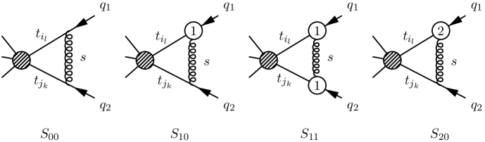
Figure 1: Sample diagrams for a soft gluon connecting two fermionic building blocks in collinear direction $i$ and $j$, respectively. The numbered vertices indicate insertions of vertices derived from the subleading power SCET Lagrangian ${\cal L}^{(n)}$ with $n=1,2$.

In this section we discuss the contribution to the anomalous dimension from soft loops. Its general structure at the one-loop order is described by the renormalization matrix $\delta Z_{PQ}^{s,ij}(y)$ defined in Eqs. (2.14) and (2.16). The first term on the right-hand side of Eq. (2.16) captures the contribution from soft loops for which all interaction vertices are derived from the leading-power SCET Lagrangian, and was discussed in Ref. [14]. An example is diagram $S_{00}$ shown in Fig. 1. In this case the power suppression arises from the currents themselves. Employing colour space operator notation allows us to write the anomalous dimension for arbitrary combinations of quark and gluon building blocks in a unified way, see Eq. (2.17).

We will therefore focus on soft one-loop diagrams that contain at least one power-suppressed interaction vertex derived from ${\cal L}^{(n)}$ with $n=1,2$. Some examples are $S_{10}$, $S_{11}$ and $S_{20}$ shown in Fig. 1. Such loops may feature divergences proportional to current operators, which describe the mixing of time-ordered products into currents, captured by the second term on the right-hand side of Eq. (2.16), i.e. by $\gamma^{ij}$ of Eq. (2.21).

Before we systematically investigate the anomalous dimension in the soft sector, we present an explicit example with a non-zero result. We do so to illustrate an unfamiliar feature of the power-suppressed SCET interactions in the position space formalism – the momentum-space Feynman rules contain derivatives of momentum conserving Dirac delta-functions. In our example, diagram $S_{11}$ shown in Fig. 1, we demonstrate how to treat this objects in practical computations. The two insertions of ${\cal L}_{\xi}^{(1)}$ lead to ${\cal O}(\lambda^{2})$ power suppression. Therefore, we can take the collinear building blocks to be leading-power fermionic operators $\propto\chi_{i}\chi_{j}$. Diagram $S_{11}$ describes the possible mixing of $\left(J^{T1}_{\chi,\xi}\right)_{i}\left(J^{T1}_{\chi,\xi}\right)_{j}$ into $A$-type currents. We consider a matrix element with two outgoing antiquarks,

$$\langle\bar{q}_{j}(q_{2})\bar{q}_{i}(q_{1})|\chi_{i\alpha}\chi_{j\beta}|0\rangle_{{\rm 1-loop},\ S_{11}}$$ (3.1)

$$= \tilde{\mu}^{2\epsilon}\int_{l,\tilde{q}_{1},\tilde{q}_{2}}\,\left(\frac{-in_{i+}\tilde{q}_{1}\frac{\not{n}_{i-}}{2}}{\tilde{q}_{1}^{2}+i\varepsilon}ig_{s}t^{a}X_{\perp i}^{\rho}n_{i-}^{\nu}(-l_{\rho}g_{\nu\mu}+l_{\nu}g_{\rho\mu})\frac{\not{n}_{i+}}{2}v_{i}(q_{1})\right)_{\!\alpha}$$

$${}\times\frac{-ig^{\mu\mu^{\prime}}}{l^{2}+i\varepsilon}\,\times\,\left(\frac{-in_{j+}\tilde{q}_{2}\frac{\not{n}_{j-}}{2}}{\tilde{q}_{2}^{2}+i\varepsilon}ig_{s}t^{a}X_{\perp j}^{\rho^{\prime}}n_{j-}^{\nu^{\prime}}(l_{\rho^{\prime}}g_{\nu^{\prime}\mu^{\prime}}-l_{\nu^{\prime}}g_{\rho^{\prime}\mu^{\prime}})\frac{\not{n}_{j+}}{2}v_{j}(q_{2})\right)_{\!\beta}\,,$$

where $v_{i}(q)$ denotes the $i$-collinear antiquark spinor satisfying $\not{n}_{i-}v_{i}(q)=0$, and we use the shorthand notation

$$\int_{l_{1},l_{2},\ldots}\equiv\int\frac{d^{d}l_{1}}{(2\pi)^{d}}\frac{d^{d}l_{1}}{(2\pi)^{d}}\ldots$$ (3.2)

for the loop integration measure in dimensional regularization with $d=4-2\epsilon$. The power-suppressed vertices arise from the interaction

$$S_{i\xi}^{(1)}=\int d^{d}x\,\bar{\chi}_{i}(x)\left(x_{\perp i}^{\mu}n_{i-}^{\nu}\,g_{s}F_{\mu\nu}^{\rm s}(x_{i-})\right)\frac{\not{n}_{i+}}{2}\chi_{i}(x),$$ (3.3)

with $x_{i-}\equiv(n_{i+}x)\frac{n_{i-}}{2}$, and the corresponding term for the direction $j$. Due to the explicit appearance of the space-time point $x^{\mu}$ in the interaction, the momentum-space vertex contains the derivative of the momentum-conserving delta functions,

$$X_{\perp i} = \frac{\partial}{\partial\tilde{q}_{1\perp i}}(2\pi)^{d}\delta^{(d)}(\tilde{q}_{1}-q_{1}-(n_{i-}l)n_{i+}/2)\,,$$

$$X_{\perp j} = \frac{\partial}{\partial\tilde{q}_{2\perp j}}(2\pi)^{d}\delta^{(d)}(\tilde{q}_{2}-q_{2}+(n_{j-}l)n_{j+}/2)\,.$$ (3.4)

Momentum conservation at the vertex can be imposed only after evaluation the derivative with respect to the momenta $\tilde{q}_{1}$ and $\tilde{q}_{2}$ of the fermion lines attached to the $i$- and $j$-collinear building blocks of the current, respectively. Note that, according to the SCET Feynman rules, only the $n_{i-}l$ projection of the loop momentum $l$ enters in the delta function derived from ${\cal L}_{i\xi}^{(1)}$, and analogously for direction $j$. The reason is that the soft field is multipole expanded around $x_{i-}$ in ${\cal L}_{i}$ as can be seen in Eq. (3.3). After partial integration the derivatives can be eliminated. Using the collinear projection property of the external spinors we obtain

$$\langle\bar{q}_{j}(q_{2})\bar{q}_{i}(q_{1})|\chi_{i\alpha}\chi_{j\beta}|0\rangle_{{\rm 1-loop},\ S_{11}}$$ (3.5)

$$= \tilde{\mu}^{2\epsilon}\int_{l}\Big{(}{\cal A}_{i\rho\alpha}^{a}\,(-n_{i-}^{\mu}g_{\perp i}^{\rho\nu}+n_{i-}^{\nu}g_{\perp i}^{\rho\mu})l_{\nu}\Big{)}\,\frac{-ig_{\mu\mu^{\prime}}}{l^{2}+i\varepsilon}\,\Big{(}(n_{j-}^{\mu^{\prime}}g_{\perp j}^{\rho^{\prime}\nu^{\prime}}-n_{j-}^{\nu^{\prime}}g_{\perp j}^{\rho^{\prime}\mu^{\prime}})l_{\nu^{\prime}}\,{\cal A}_{j\rho^{\prime}\beta}^{a}\Big{)},$$

where

$${\cal A}_{i\rho\alpha}^{a} = -\frac{\partial}{\partial\tilde{q}_{1\perp i}^{\rho}}\frac{n_{i+}\tilde{q}_{1}}{\tilde{q}_{1}^{2}+i\varepsilon}\Bigg{|}_{\tilde{q}_{1}=q_{1}+\frac{1}{2}(n_{i-}l)n_{i+}}g_{s}t^{a}v_{i\alpha}(q_{1})\,,$$

$${\cal A}_{j\rho^{\prime}\beta}^{a} = -\frac{\partial}{\partial\tilde{q}_{2\perp j}^{\rho^{\prime}}}\frac{n_{j+}\tilde{q}_{2}}{\tilde{q}_{2}^{2}+i\varepsilon}\Bigg{|}_{\tilde{q}_{2}=q_{2}-\frac{1}{2}(n_{j-}l)n_{j+}}g_{s}t^{a}v_{j\beta}(q_{2})\,.$$ (3.6)

The integrand has the structure $l^{\nu}l^{\nu^{\prime}}F(n_{i-}l,n_{j-}l,l^{2})$ with some scalar function $F$. There is no explicit dependence on $l_{\perp}$, since after the derivative with respect to $\tilde{q}_{1\perp i}^{\rho}$ ($\tilde{q}_{2\perp j}^{\rho^{\prime}}$) is carried out $\tilde{q}_{1}^{2}$ ($\tilde{q}_{2}^{2}$) is set to $q_{1}^{2}+n_{i-}ln_{i+}q_{1}$ ($q_{2}^{2}-n_{j-}ln_{j+}q_{2}$). Therefore the integral can be decomposed, after integration, into terms proportional to the tensors $n_{i-}^{\nu}n_{i-}^{\nu^{\prime}}$, $n_{j-}^{\nu}n_{j-}^{\nu^{\prime}}$, $n_{i-}^{\nu}n_{j-}^{\nu^{\prime}}$, $n_{j-}^{\nu}n_{i-}^{\nu^{\prime}}$, and $g^{\nu\nu^{\prime}}$. By making an ansatz of a linear combination of these tensors, and contracting with them, one finds that one can replace inside of the integrand

$$l^{\nu}l^{\nu^{\prime}} \mapsto \frac{1}{d-2}\left(l^{2}-2\frac{n_{i-}l\,n_{j-}l}{n_{i-}n_{j-}}\right)g^{\nu\nu^{\prime}}-\frac{1}{d-2}\left(l^{2}-d\frac{n_{i-}l\,n_{j-}l}{n_{i-}n_{j-}}\right)\frac{n_{i-}^{\nu}n_{j-}^{\nu^{\prime}}+n_{i-}^{\nu^{\prime}}n_{j-}^{\nu}}{n_{i-}n_{j-}}$$ (3.7)

$${}+\left(\frac{n_{j-}l}{n_{i-}n_{j-}}\right)^{2}n_{i-}^{\nu}n_{i-}^{\nu^{\prime}}+\left(\frac{n_{i-}l}{n_{i-}n_{j-}}\right)^{2}n_{j-}^{\nu}n_{j-}^{\nu^{\prime}}\,.$$

The terms $\propto l^{2}$ vanish, since the gluon propagator $1/(l^{2}+i\varepsilon)$ is cancelled, resulting in an infrared finite and quadratically ultraviolet divergent scaleless transverse momentum integral, which does not contribute to the anomalous dimension. Furthermore, since $\nu$ is contracted with either a $\perp$ vector in the $i$ direction or with $n_{i-}$, terms $\propto n_{i-}^{\nu}$ vanish. Similarly, terms $\propto n_{j-}^{\nu^{\prime}}$ vanish. Inserting this decomposition in Eq. (3.5) yields

$$\langle\bar{q}_{j}(q_{2})\bar{q}_{i}(q_{1})|\chi_{i\alpha}\chi_{j\beta}|0\rangle_{{\rm 1-loop},\ S_{11}}$$

$$= -4ig_{s}^{2}\tilde{\mu}^{2\epsilon}\,\frac{4-d}{d-2}\,\frac{(q_{1\perp i}q_{2\perp j})(n_{i-}n_{j-})-(n_{i-}q_{2\perp j})(n_{j-}q_{1\perp i})}{n_{i-}n_{j-}}\Big{(}t^{a}v_{i\alpha}(q_{1})\Big{)}\Big{(}t^{a}v_{j\beta}(q_{2})\Big{)}$$

$$\times\int_{l}\,\frac{n_{i+}q_{1}n_{i-}l}{(q_{1}^{2}-n_{i+}q_{1}n_{i-}l+i\varepsilon)^{2}}\,\frac{1}{l^{2}+i\varepsilon}\,\frac{n_{j+}q_{2}n_{j-}l}{(q_{2}^{2}+n_{j+}q_{2}n_{j-}l+i\varepsilon)^{2}}$$

$$= -\frac{1}{\epsilon}\,\frac{2\alpha_{s}}{\pi}\,\frac{(q_{1\perp i}q_{2\perp j})(n_{i-}n_{j-})-(n_{i-}q_{2\perp j})(n_{j-}q_{1\perp i})}{n_{i+}q_{1}n_{j+}q_{2}(n_{i-}n_{j-})^{2}}\Big{(}t^{a}v_{i\alpha}(q_{1})\Big{)}\Big{(}t^{a}v_{j\beta}(q_{2})\Big{)}+{\cal O}(\epsilon^{0})\,,$$

where we used the master integral from App. B in the last step. Note the explicit factor $4-d=2\epsilon$ in the first line, which cancels the double pole from the integral. The remaining $1/\epsilon$ divergence can be absorbed by a counterterm proportional to the current $\left(J^{A1}_{\partial^{\mu}\chi}\right)_{i}\left(J^{A1}_{\partial^{\nu}\chi}\right)_{j}=[i\partial_{\perp i}^{\mu}\chi_{i}][i\partial_{\perp j}^{\nu}\chi_{j}]$, resulting in the non-vanishing entry

$$\gamma^{ij}_{\left(J^{T1}_{\chi,\xi}\right)_{i}\left(J^{T1}_{\chi,\xi}\right)_{j},\left(J^{A1}_{\partial^{\mu}\chi}\right)_{i}\left(J^{A1}_{\partial^{\nu}\chi}\right)_{j}}={}\frac{2\alpha_{s}}{\pi}\,{\bf T}_{i}\cdot{\bf T}_{j}\,G^{\mu\nu}_{ij}\,,$$ (3.9)

of the anomalous dimension matrix, where

$$G^{\mu\nu}_{ij}\equiv\left(g^{\mu\nu}-\frac{n_{i-}^{\nu}n_{j-}^{\mu}}{n_{i-}n_{j-}}\right)\frac{1}{(n_{i-}n_{j-})P_{i}P_{j}}\,.$$ (3.10)

Here we omitted the building blocks belonging to the $N-2$ collinear directions different from $i$ and $j$, which remain unchanged, as well as Dirac indices, since the above anomalous dimension is diagonal in them in each collinear direction. This computation also implies that

$$\gamma^{ij}_{\left(J^{T1}_{\chi,\xi}\right)_{i}\left(J^{T1}_{\chi,\xi}\right)_{j},\left(J^{A2}_{\partial^{\mu}\partial^{\nu}\chi}\right)_{i}\left(J^{A0}_{\chi}\right)_{j}}={}0\,,$$ (3.11)

and analogously for $J^{A2}\leftrightarrow J^{A0}$. The computation above was done in Feynman gauge. Independence on the gauge-fixing parameter in general covariant gauge is easily seen from Eq. (3.1), since replacing $g^{\mu\mu^{\prime}}\to l^{\mu}l^{\mu^{\prime}}/l^{2}$ produces zero upon contracting $l^{\mu}$ with the vertex factor. The reason for this is that the soft-gluon vertex in ${\cal L}^{(1)}_{\xi}$ comes from the field strength tensor. We also note that with our conventions off-diagonal elements of the anomalous dimension matrix need not be dimensionless as is apparent from the result (3.10). In this way we avoid putting explicit factors of the hard scale into the generic operator basis. For the special case of back-to-back directions, $n_{j-}=n_{i+}$, and, since $\mu$, $\nu$ are contracted with transverse vectors, $G_{ij}^{\mu\nu}$ simplifies to $g_{\perp}^{\mu\nu}/(2Q^{2})$, where $Q^{2}=P_{i}P_{j}$ is the invariant mass of the particles in the back-to-back directions, resulting in a simple expression for the soft mixing anomalous dimension (3.9).

In order to determine the mixing into $B$- and $C$-type currents, as well as of different types of time-ordered products, we need to consider matrix elements with one or two additional collinear emissions in direction $i$ or $j$. To simplify this computation, we consider the general structure of soft loops, depending on the number and type of insertions of power-suppressed interactions. We first consider the case of a single ${\cal L}^{(1)}$ insertion, then a double ${\cal L}^{(1)}$ insertion, and finally a single ${\cal L}^{(2)}$ insertion, for the case $F_{i}=F_{j}=+1$. The results for fermion number $(F_{i},F_{j})=(+1,+1)$ can be generalized straightforwardly to operators with $\bar{\chi}$ instead of $\chi$ building blocks, i.e. $(F_{i},F_{j})=(-1,-1),(1,-1),(-1,1)$, see App. D.

3.1 Single insertion of ${\cal L}^{(1)}$

In Ref. [14] it has been shown that soft loops with a single insertion of ${\cal L}^{(1)}$ vanish for the case $F_{i}=\pm 2$. We now generalize this result to currents with arbitrary fermion number (such as in diagram $S_{10}$ in Fig. 1). We consider an operator containing a single time-ordered product involving an insertion of ${\cal L}^{(1)}$ along direction $i$. This operator can potentially mix into current operators containing, instead of the time-ordered product, either an extra transverse derivative or an extra collinear building block along one of the $N$ collinear directions. To determine this mixing it is therefore sufficient to consider a soft loop diagram with a soft line connecting direction $i$ with any other direction $j$, and with up to one extra collinear emission. The vertex to which the soft line is attached along direction $j$ is a leading-power interaction. Since soft quarks do not interact with collinear particles at leading power, only the case of a soft gluon line needs to be considered. This implies in turn that the power-suppressed interaction along direction $i$ has to contain a soft gluon as well, i.e. we need to consider only ${\cal L}_{\xi}^{(1)}$ or ${\cal L}_{\rm YM}^{(1)}$. Operators containing a single time-ordered product involving ${\cal L}_{\xi q}^{(1)}$ cannot mix into currents.

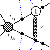
Figure 2: Generic soft one-loop diagram featuring a single insertion of ${\cal L}_{\xi}^{(1)}$ or ${\cal L}_{\rm YM}^{(1)}$ along collinear direction $i$, a leading-power interaction along direction $j$, and a soft gluon exchanged between them. Solid lines without arrow can be either collinear quarks or gluons. Dotted lines illustrate possible additional collinear emissions (additional emissions directly off the current are not shown). The relevant diagrams are obtained by choosing one emission out of the dashed lines, or none for the case without extra emission.

A generic soft loop diagram of the type described above is shown in Fig. 2. Here dotted lines illustrate possible attachments of an extra collinear emission. As stated in the previous paragraph, only one extra emission needs to be considered. This emission can be attached to either direction $i$ or $j$. In addition, it can be either off an internal or external propagator, or off one of the vertices involving the soft gluon. Extra emission directly off the current is also possible, but not shown for brevity.

It turns out that the loop amplitudes for all relevant diagrams can be written in a generic form. Let us assume that the soft gluon line carries momentum $l$. The leading-power interaction is proportional to $n_{j-}^{\mu^{\prime}}$ for all vertices involving a soft gluon, since soft gluons enter only via the projection $n_{-}D$ of the covariant derivative into the leading-power collinear Lagrangian. The power suppressed interaction vertices derived from both ${\cal L}_{\xi}^{(1)}$ or ${\cal L}_{\rm YM}^{(1)}$ contribute the factor

$$n_{i-}l\,g_{\perp i}^{\rho\mu}-n_{i-}^{\mu}l_{\perp i}^{\rho}=(n_{i-}^{\nu}g_{\perp i}^{\rho\mu}-n_{i-}^{\mu}g_{\perp i}^{\rho\nu})l_{\nu}\,,$$ (3.12)

where the index $\rho$ is contracted either with a derivative with respect to a $\perp$ momentum or, for the 4-gluon vertex, with the $\perp$ component of some collinear momentum. The reason is that at ${\cal O}(\lambda)$ the soft field enters the collinear SCET Lagrangian only via the soft field strength tensor projected in the $-$ and $\perp$ directions, $n_{-}^{\nu}F^{s}_{\nu\kappa_{\perp}}$. Restricting for the moment to the time-ordered product with a leading-power current, the loop amplitude in Feynman gauge can be written in the form

$$\langle f|\chi_{i\alpha}\chi_{j\beta}|0\rangle_{\,{\rm single}\ {\cal L}^{(1)}\ {\rm insertion}}=\tilde{\mu}^{2\epsilon}\int_{l}\Big{(}{\cal A}_{i\rho\alpha}^{a}\,(n_{i-}^{\nu}g_{\perp i}^{\rho\mu}-n_{i-}^{\mu}g_{\perp i}^{\rho\nu})l_{\nu}\Big{)}\,\frac{-ig_{\mu\mu^{\prime}}}{l^{2}+i\varepsilon}\,\Big{(}n_{j-}^{\mu^{\prime}}{\cal A}_{j\beta}^{a}\Big{)}\,,$$ (3.13)

where ${\cal A}_{i\rho\alpha}^{a}$ and ${\cal A}_{j\beta}^{a}$ denote the pieces of the amplitude involving propagators and vertices along direction $i$ and $j$, respectively, and $a$ refers to the colour index of the soft gluon. Furthermore, $\langle f|\in\{\langle\bar{q}_{j}\bar{q}_{i}|,\langle\bar{q}_{j}g_{j}\bar{q}_{i}|,\langle\bar{q}_{j}\bar{q}_{i}g_{i}|\}$ stands for states with either two outgoing antiquarks, or with an extra collinear gluon in direction $i$ or $j$. For example, for the particular case without additional collinear emission ${\cal A}_{i\rho\alpha}^{a}$ is given by Eq. (3) and

$${\cal A}_{j\beta}^{a}\Big{|}_{\rm no\ extra\ emission}\ =\ \frac{n_{j+}q_{2}}{q_{2}^{2}-n_{j+}q_{2}n_{j-}l+i\varepsilon}g_{s}t^{a}v_{j\beta}(q_{2})\,.$$ (3.14)

Note that, also in the general case, ${\cal A}_{i\rho\alpha}^{a}$ depends on the loop momentum only via $n_{i-}l$, and ${\cal A}_{j\beta}^{a}$ only via $n_{j-}l$, due to the multipole expansion.

The loop integrand has the structure $l^{\nu}F(n_{i-}l,n_{j-}l,l^{2})$, such that by analogous reasoning as for the example above, the integral can be decomposed in contributions proportional to $n_{i-}^{\nu}$ and $n_{j-}^{\nu}$. Inside the loop integrand one may replace

$$l^{\nu}\mapsto\frac{n_{j-}l}{n_{j-}n_{i-}}n_{i-}^{\nu}+\frac{n_{i-}l}{n_{j-}n_{i-}}n_{j-}^{\nu}\;.$$ (3.15)

The former term on the right-hand side vanishes since $n_{i-}^{2}=0$ and $g_{\perp i}^{\rho\nu}{n_{i-}}_{\nu}=0$. The latter vanishes since $(n_{i-}^{\nu}g_{\perp i}^{\rho\mu}-n_{i-}^{\mu}g_{\perp i}^{\rho\nu}){n_{j-}}_{\nu}{n_{j-}}_{\mu}=0$. Therefore, operators containing a single time-ordered product involving an ${\cal L}^{(1)}$ insertion do not mix into local currents. This generalizes the argument of Ref. [14] to operators with $F_{i}=F_{j}=+1$, and implies at ${\cal O}(\lambda)$

$$\gamma^{ij}_{\left(J^{T1}_{\chi,V}\right)_{i}\left(J^{A0}_{\chi}\right)_{j},\left(J^{A1}_{\partial\chi}\right)_{i}\left(J^{A0}_{\chi}\right)_{j}}=\gamma^{ij}_{\left(J^{T1}_{\chi,V}\right)_{i}\left(J^{A0}_{\chi}\right)_{j},\left(J^{B1}_{{\cal A}\chi}\right)_{i}\left(J^{A0}_{\chi}\right)_{j}}=0\,,$$ (3.16)

for $V\in\{\xi,{\rm YM},\xi q\}$. Adding transverse derivatives or collinear building blocks to the operator does not affect the general form of the soft loop integral, since after the transverse momentum derivatives from the vertices have been done, the denominator of the integrand depends only on the $n_{i-}l$ and $n_{j-}l$ components of the loop momentum, and since at most one factor of $l_{\perp}$ can appear in the numerator. Therefore, we conclude that at ${\cal O}(\lambda^{2})$

$$\gamma^{ij}_{\left(J^{T2}_{\partial\chi,V}\right)_{i}\left(J^{A0}_{\chi}\right)_{j},J^{\prime}_{i}J^{\prime}_{j}}=\gamma^{ij}_{\left(J^{T2}_{{\cal A}\chi,V}\right)_{i}\left(J^{A0}_{\chi}\right)_{j},J^{\prime}_{i}J^{\prime}_{j}}=\gamma^{ij}_{\left(J^{T1}_{\chi,V}\right)_{i}\left(J^{A1}_{\partial\chi}\right)_{j},J^{\prime}_{i}J^{\prime}_{j}}=\gamma^{ij}_{\left(J^{T1}_{\chi,V}\right)_{i}\left(J^{B1}_{{\cal A}\chi}\right)_{j},J^{\prime}_{i}J^{\prime}_{j}}=0\,,$$ (3.17)

where $J^{\prime}_{i}J^{\prime}_{j}$ is a product of arbitrary local currents in directions $i$ and $j$. Once again, gauge invariance is a trivial consequence of the structure of the SCET power-suppressed soft-gluon vertices.

We also note that the loop amplitude has the same structure for operators containing gluon building blocks. Thus Eq. (3.17) remains true, when $\chi$ in $J^{T1}$, $J^{T2}$ and/or $J^{A0}_{\chi}$ is replaced by ${\cal A}$ – the single insertions with ${\cal L}^{(1)}$ never contribute to the one-loop anomalous dimension matrix to $\mathcal{O}(\lambda^{2})$.

3.2 Double insertion of ${\cal L}^{(1)}$

There are two types of operators containing a double insertion of ${\cal L}^{(1)}$. Either both insertions belong to the same collinear direction (involving $J^{T2}_{\chi,VW}$), or the two insertions belong to different directions (involving $J^{T1}_{\chi,V}J^{T1}_{\chi,W}$). We consider the two cases in turn.

3.2.1 Double insertion in a single collinear direction

Diagrams containing a double time-ordered product along a single collinear direction, say $i$, can potentially mix into local currents at the one-loop order by connecting the two insertions with a soft line. This leads to loop integrals of the form

$$\int_{l}\,\frac{l^{\mu}l^{\nu}\cdots}{l^{2}+i\varepsilon}\prod_{a}\frac{1}{p_{a}^{2}-n_{i+}p_{a}n_{i-}l+i\varepsilon}\,,$$ (3.18)

where $p_{a}$ are linear combinations of collinear momenta in direction $i$, and $p_{a}^{2}\not=0$ due to the off-shell regularization. The momentum derivatives contained in the SCET Feynman rules do not change this general structure. If some of the $p_{a}$ are identical, higher powers of the propagator occur, which can be related to an integral with a single power, differentiated with respect to $p_{a}^{2}$.

We now show that the above integrals always vanish. Note that the integrand has only a single pole at $n_{i+}l=-(l_{\perp i}^{2}+i\varepsilon)/n_{i-}l$, but closing the contour in the half plane that does not contain this pole, does not allow us to conclude that the integral is zero, since the integral over the half-circle at infinity is not convergent. On the other hand, inspection of the diagrams shows that an additional factor of $l^{\mu}$ is accompanied by an additional denominator containing $n_{i-}l$ such that the $n_{i-}l$ integral over the infinite circle is always zero. Hence, when $n_{i+}l>0$ we pick up the residues in the upper $n_{i-}l$ half plane at $n_{i-}l=p_{a}^{2}/n_{i+}p_{a}+i\varepsilon$ ($n_{i+}p$ is positive), while the integral vanishes for $n_{i+}l<0$, when all poles lie in the positive half plane. This converts the loop integral into a sum of terms of the form

$$\int_{0}^{\infty}dn_{i+}l\int d^{d-2}l_{\perp i}\,\frac{(n_{i+}l)^{b}\,l_{\perp i}^{\mu}l_{\perp i}^{\nu}\ldots}{\frac{n_{i+}l}{n_{i+}p_{a}}\,p_{a}^{2}+l_{\perp i}^{2}+i\varepsilon}$$ (3.19)

with non-negative $b$. Performing the dimensionally regulated transverse momentum integral results in $n_{i+}l$ integrals of the form

$$\int_{0}^{\infty}dn_{i+}l\left(n_{i+}l\right)^{b-\epsilon},\;\;b\geq 0$$ (3.20)

with some other non-negative $b$ and neglecting any $l$ independent prefactors. These scaleless integrals are IR finite and develop power-like divergences in the UV region. Even though the integral over $l_{\perp}$ may generate a $\frac{1}{\epsilon}$ pole, the result is zero due to the vanishing scaleless $n_{i+}l$ integral as was to be shown. Hence, soft one-loop diagrams within a single collinear direction do not contribute to the anomalous dimension at any power of $\lambda$. In particular,

$$\gamma^{ij}_{\left(J^{T2}_{\chi,VW}\right)_{i}\left(J^{A0}_{\chi}\right)_{j},J^{\prime}_{i}J^{\prime}_{j}}=0$$ (3.21)

for $V,W\in\{\xi,{\rm YM},\xi q\}$, and by the same argument

$$\gamma^{ij}_{T(P,{\cal L}^{(1)}_{k},{\cal L}^{(1)}_{k}),Q}=0$$ (3.22)

for $i,j,k=1,\dots,N$ and arbitrary local $N$-jet operators $P$, $Q$.

3.2.2 Double insertion in different collinear directions

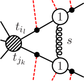
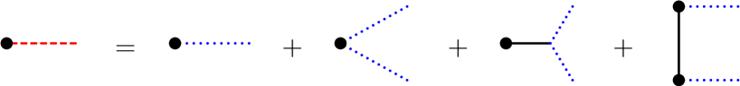
Figure 3: Generic soft one-loop diagram featuring a double insertion of ${\cal L}_{\xi}^{(1)}$ or ${\cal L}_{\rm YM}^{(1)}$ along collinear directions $i$ and $j$, respectively. Solid lines without arrow can be either collinear quarks or gluons. Dashed lines illustrate possible sub-diagrams with additional collinear emissions (additional emissions directly off the current are not shown). In the second line, we show possible sub-diagrams. Only diagrams that contain at most two dotted lines, i.e. two collinear emissions, need to be considered.

We next consider a double time-ordered product operator with one insertion of ${\cal L}^{(1)}_{i}$ in direction $i$ and one of ${\cal L}^{(1)}_{j}$ in another direction $j$. One-loop mixing with a current operator can occur when both insertions are connected by a soft line. For the moment we focus on the case of a soft gluon line and refer to Sec. 3.4 for the case of soft quark mixing. Therefore we consider insertions of ${\cal L}_{\xi}^{(1)}$ or ${\cal L}_{\rm YM}^{(1)}$. The corresponding operators contain two time-ordered products $\left(J^{T1}_{\chi,V}\right)_{i}\left(J^{T1}_{\chi,W}\right)_{j}$ with $V,W\in\{\xi,{\rm YM}\}$, which can mix into currents with two additional $\perp$ derivatives, or two additional building blocks, or one $\perp$ derivative together with one extra building block. Accordingly, we analyze diagrams with up to two additional collinear emissions. Such diagrams are summarized in Fig. 3. No more than two of the dashed lines should be replaced by one of the dotted subdiagrams shown in the second line, such that the resulting diagram contains at most two dotted lines. Emissions directly off the current are not shown for simplicity. The ${\cal L}^{(1)}$ insertion in direction $i$ contributes a factor of the form (3.12), and a corresponding factor arises for direction $j$ with opposite sign since the direction of the soft momentum is reversed. The amplitude for all relevant diagrams can therefore be written in the form

$$\langle f|\chi_{i\alpha}\chi_{j\beta}|0\rangle_{\,{\rm double}\ {\cal L}^{(1)}\ {\rm insertion}}$$ (3.23)

$$= \tilde{\mu}^{2\epsilon}\int_{l}\Big{(}{\cal A}_{i\rho\alpha}^{a}\,(-n_{i-}^{\mu}g_{\perp i}^{\rho\nu}+n_{i-}^{\nu}g_{\perp i}^{\rho\mu})l_{\nu}\Big{)}\,\frac{-ig_{\mu\mu^{\prime}}}{l^{2}+i\varepsilon}\,\Big{(}(n_{j-}^{\mu^{\prime}}g_{\perp j}^{\rho^{\prime}\nu^{\prime}}-n_{j-}^{\nu^{\prime}}g_{\perp j}^{\rho^{\prime}\mu^{\prime}})l_{\nu^{\prime}}\,{\cal A}_{j\rho^{\prime}\beta}^{a}\Big{)}\,,\qquad$$

where ${\cal A}_{i\rho\alpha}^{a}$ ( ${\cal A}_{j\rho^{\prime}\beta}^{a}$) contains collinear propagators and vertices in direction $i$ ($j$). For the case without extra collinear emission they are given by Eq. (3), and we recover Eq. (3.5). The external states for up to two additional collinear emissions are

$$\langle f|\in\{\langle\bar{q}_{j}\bar{q}_{i}|,\langle\bar{q}_{j}g_{j}\bar{q}_{i}|,\langle\bar{q}_{j}\bar{q}_{i}g_{i}|,\langle\bar{q}_{j}g_{j}\bar{q}_{i}g_{i}|,\langle\bar{q}_{j}g_{j}g^{\prime}_{j}\bar{q}_{i}|,\langle\bar{q}_{j}\bar{q}_{i}g_{i}g_{i}^{\prime}|,\langle\bar{q}_{j}q_{j}^{\prime}\bar{q}_{j}^{\prime\prime}\bar{q}_{i}|,\langle\bar{q}_{j}\bar{q}_{i}q_{i}^{\prime}\bar{q}_{i}^{\prime\prime}|\,\}\,.$$ (3.24)

The four-fermion states $\langle\bar{q}_{j}q_{j}^{\prime}\bar{q}_{i}\bar{q}_{i}^{\prime}|$ and $\langle\bar{q}_{j}\bar{q}_{j}^{\prime}\bar{q}_{i}q_{i}^{\prime}|$ could contribute only in conjunction with soft fermion exchange diagrams and ${\cal L}^{(1)}_{\xi q}$ insertions, which will be discussed separately in Sec. 3.4. Since ${\cal A}_{i\rho\alpha}^{a}$ and ${\cal A}_{j\rho^{\prime}\beta}^{a}$ depend on the loop momentum only via $n_{i-}l$ and $n_{j-}l$, respectively, the loop integral can be decomposed using Eq. (3.7) and we obtain

$$\langle f|\chi_{i\alpha}\chi_{j\beta}|0\rangle_{\,{\rm double}\ {\cal L}^{(1)}\ {\rm insertion}}$$ (3.25)

$$= -ig_{s}^{2}\tilde{\mu}^{2\epsilon}\,\frac{4-d}{d-2}\,\left(g_{\lambda\lambda^{\prime}}-\frac{{n_{i-}}_{\lambda^{\prime}}{n_{j-}}_{\lambda}}{n_{i-}n_{j-}}\right)g_{\perp i}^{\lambda\rho}g_{\perp j}^{\lambda^{\prime}\rho^{\prime}}\,\int_{l}\,{\cal A}_{i\rho\alpha}^{a}\,\frac{n_{i-}ln_{j-}l}{l^{2}+i\varepsilon}\,{\cal A}_{j\rho^{\prime}\beta}^{a}\,.$$

For $d\to 4$ the loop integral generically has a double $1/\epsilon^{2}$ pole, but due to the prefactor the complete amplitude has only a single pole. A large number of a priori possible mixings can now be eliminated by two general considerations:

• The loop integral depends on two additional Lorentz indices $\rho_{\perp i}$ and $\rho^{\prime}_{\perp j}$, projected along the $\perp$ directions with respect to $i$ and $j$. The possible $\perp$ vectors entering ${\cal A}_{i\rho\alpha}^{a}$ are a) the external momenta of $i$-collinear particles, b) the polarization vectors of $i$-collinear gluons, or c) $\gamma_{\perp i}^{\rho}$. Case a) implies mixing into an $A1$ operator $J_{i}^{A1}$, b) a $B1$ operator $J_{i}^{B1}$ and the same is true for case c) for the following reason: Inspecting the Feynman rules Eqs. (A.28), (A.29) and (A.32), one finds that $\gamma_{\perp i}^{\rho}$ may enter in ${\cal A}_{i\rho\alpha}^{a}$ only in connection to vertices involving extra collinear emissions in direction $i$. Analogous properties hold for direction $j$. Together with power counting in $\lambda$, this implies that the divergent part can be absorbed by a counterterm containing either an extra derivative or an extra building block in both the $i$ as well as the $j$ direction. This means that only mixings of the form

  $$\left(J^{T1}_{\chi,V}\right)_{i}\left(J^{T1}_{\chi,W}\right)_{j}\to J^{X1}_{i}J^{Y1}_{j}$$ (3.26)

  are possible, i.e. into a product of ${\cal O}(\lambda)$ currents in both directions (with $X,Y=A,B$), but not mixing into e.g. $J^{X2}_{i}J^{A0}_{j}$ ($X=A,B,C$). This generalizes the result obtained earlier in Eq. (3.11).

• The insertion ${\cal L}_{\rm YM}^{(1)}$ can give non-zero matrix elements only if an additional collinear gluon appears in the final state (see diagrams in Fig. 5 below). To renormalize such a diagram by a current without gluon building block, such as $[\partial_{\perp i}\chi_{i}][\partial_{\perp j}\chi_{j}]$, would require a collinear emission from a Wilson line. There are two arguments why this cannot happen: (i) in the light-cone gauge such diagrams do not exist. (ii) suppose one would have to introduce a counterterm proportional to $[\partial_{\perp i}\chi_{i}][\partial_{\perp j}\chi_{j}]$ to renormalize a one-loop diagram containing $(J^{T1}_{\chi,{\rm YM}})_{i}(J^{T1}_{\chi,{\rm YM}})_{j}$. Then one could compute the corresponding diagram without extra emission. In this case the tree-level diagram with the counterterm is non-zero, while the one-loop diagram with $(J^{T1}_{\chi,{\rm YM}})_{i}(J^{T1}_{\chi,{\rm YM}})_{j}$ vanishes. This contradicts the property that, once the counterterm is fixed, all possible matrix elements have to be finite. This argument implies also that

  $$\left(J^{Tn}_{\chi,{\rm YM}}\right)_{i}J_{j}\to\left[\partial_{\perp i}^{\mu_{1}}\ldots\partial_{\perp i}^{\mu_{n}}\chi_{i}\right]J_{j}^{\prime}$$ (3.27)

  vanishes, where $J_{j},J_{j}^{\prime}$ can be arbitrary currents or time-ordered products. For example, $\left(J^{T1}_{\chi,{\rm YM}}\right)_{i}\left(J^{T1}_{\chi,{\rm YM}}\right)_{j}\to[\partial_{\perp i}\chi_{i}]({\cal A}\chi)_{j}$ mixing does not occur.

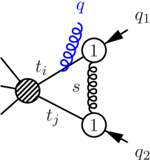
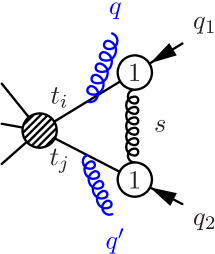
Figure 4: Relevant diagrams for the mixing $\left(J_{\chi,\xi}^{T1}\right)_{i}\left(J_{\chi,\xi}^{T1}\right)_{j}\to J^{B1}_{i}J^{A1}_{j}$ (left) and $\left(J_{\chi,\xi}^{T1}\right)_{i}\left(J_{\chi,\xi}^{T1}\right)_{j}\to J^{B1}_{i}J^{B1}_{j}$ (right).

The only possible mixings of two time-ordered products into currents with $F_{i}=F_{j}=1$ are therefore

• $\left(J_{\chi,\xi}^{T1}\right)_{i}\left(J_{\chi,\xi}^{T1}\right)_{j}\to J^{X1}_{i}J^{Y1}_{j}$ ,

• $\left(J_{\chi,{\rm YM}}^{T1}\right)_{i}\left(J_{\chi,\xi}^{T1}\right)_{j}\to J^{B1}_{i}J^{Y1}_{j}$ ,

• $\left(J_{\chi,{\rm YM}}^{T1}\right)_{i}\left(J_{\chi,{\rm YM}}^{T1}\right)_{j}\to J^{B1}_{i}J^{B1}_{j}$ ,

with $X,Y=A,B$ (in the middle line the case with $i\leftrightarrow j$ is analogous). This reduces the number of states $\langle f|$ that need to be considered to compute the anomalous dimension to the first four in Eq. (3.24). The mixing $\left(J_{\chi,\xi}^{T1}\right)_{i}\left(J_{\chi,\xi}^{T1}\right)_{j}\to J^{A1}_{i}J^{A1}_{j}$ has been treated already, and the result is given in Eq. (3.9). For $\left(J_{\chi,\xi}^{T1}\right)_{i}\left(J_{\chi,\xi}^{T1}\right)_{j}\to J^{B1}_{i}J^{A1}_{j}$ we consider the matrix element with $\langle f|=\langle\bar{q}_{j}\bar{q}_{i}g_{i}|$. To extract the operator mixing it is sufficient to let the gluon have $\perp$ polarization, and assume $(q_{1})_{\perp i}=q_{\perp i}=0$. Then the only non-zero diagram is shown in Fig. 4 (left). The diagram with gluon emission off the power-suppressed vertex vanishes for $\perp$ polarization, and with emission off the external quark line because $(q_{1})_{\perp i}=q_{\perp i}=0$. In this case ${\cal A}_{j\rho^{\prime}\beta}^{a}$ is given by Eq. (3) and

$${\cal A}_{i\rho\alpha}^{a} = -\frac{\partial}{\partial\tilde{q}_{1\perp i}^{\rho}}\Bigg{[}\frac{n_{i+}(\tilde{q}_{1}+q)}{(\tilde{q}_{1}+q)^{2}+i\varepsilon}$$ (3.28)

$${}\times\left(\frac{\not{\tilde{q}}_{1\perp i}\not{\epsilon}^{*}_{\perp i}}{n_{i+}(\tilde{q}_{1}+q)}+\frac{\not{\epsilon}^{*}_{\perp i}\not{\tilde{q}}_{1\perp i}}{n_{i+}\tilde{q}_{1}}\right)\frac{n_{i+}\tilde{q}_{1}}{\tilde{q}_{1}^{2}+i\varepsilon}g_{s}^{2}t^{b}t^{a}v_{i}(q_{1})\Bigg{]}_{\alpha}\Bigg{|}_{\tilde{q}_{1}=q_{1}+\frac{1}{2}(n_{i-}l)n_{i+}}\,.$$

For $q_{1\perp i}=0$ a non-zero contribution arises when the derivative acts on $\not{\tilde{q}}_{1\perp i}$. In collinear momentum space, we obtain using Eq. (3.25) and App. B

$$\langle\bar{q}_{j}\bar{q}_{i}g_{i}^{b}|\left(J_{\chi_{\alpha},\xi}^{T1}\right)_{i}\left(J_{\chi_{\beta},\xi}^{T1}\right)_{j}|0\rangle = P_{i}\delta(P_{i}-n_{i+}(q_{1}+q))P_{j}\delta(P_{j}-n_{j+}q_{2})$$ (3.29)

$${}\times{\cal M}_{\alpha\beta,\gamma\delta}^{\mu\nu}\epsilon_{\mu\perp i}^{*}(q)\left(t^{b}t^{a}v_{i\gamma}(q_{1})\right)(q_{2})_{\nu\perp j}(t^{a}v_{j\delta}(q_{2}))\,,\qquad$$

with

$${\cal M}_{\alpha\beta,\gamma\delta}^{\mu\nu}=\frac{g_{s}^{3}}{4\pi^{2}\epsilon}\frac{(n_{i-}n_{j-})g^{\lambda\nu}-n_{i-}^{\nu}n_{j-}^{\lambda}}{n_{j+}q_{2}(n_{i-}n_{j-})^{2}}\left(\frac{\gamma_{\lambda\perp i}\gamma_{\perp i}^{\mu}}{n_{i+}(q_{1}+q)}+\frac{\gamma_{\perp i}^{\mu}\gamma_{\lambda\perp i}}{n_{i+}q_{1}}\right)_{\alpha\gamma}\delta_{\beta\delta}+{\cal O}(\epsilon^{0})\,.$$ (3.30)

The tree-level matrix element of the $({\cal A}\chi)_{i}i\partial_{\perp j}\chi_{j}$ operator is

$$\langle\bar{q}_{j}\bar{q}_{i}g_{i}^{a}|\left(J^{B1}_{{\cal A}^{\mu}_{b}\chi_{\gamma}}(y)\right)_{i}\,\left(J^{A1}_{\partial^{\nu}\chi_{\delta}}\right)_{j}|0\rangle_{\rm tree} = P_{i}^{2}\delta(yP_{i}-n_{i+}q)\delta(\bar{y}P_{i}-n_{i+}q_{1})\,P_{j}\delta(P_{j}-n_{j+}q_{2})$$ (3.31)

$${}\times g_{s}\delta_{ab}\epsilon_{\perp i}^{*\mu}(q)v_{i\gamma}(q_{1})\,(-q_{2}^{\nu})_{\perp j}v_{j\delta}(q_{2})\,,$$

where $y$ is the collinear momentum fraction carried by the first building block in direction $i$ (i.e. the gluon) and $\bar{y}=1-y$. Comparing the two expressions, we find the operator mixing

$$\left(J_{\chi_{\alpha},\xi}^{T1}\right)_{i}\left(J_{\chi_{\beta},\xi}^{T1}\right)_{j} \to \frac{\alpha_{s}}{\pi\epsilon}\int_{0}^{1}dy\,{\bf T}^{b}_{i}\,({\bf T}_{i}\cdot{\bf T}_{j})G_{\lambda\nu}^{ij}$$ (3.32)

$${}\times\left(\gamma_{\perp i}^{\lambda}\gamma_{\perp i}^{\mu}+\frac{\gamma_{\perp i}^{\mu}\gamma_{\perp i}^{\lambda}}{\bar{y}}\right)_{\alpha\gamma}\delta_{\beta\delta}\left(J^{B1}_{{\cal A}_{\mu}^{b}\chi_{\gamma}}(y)\right)_{i}\,\left(J^{A1}_{\partial^{\nu}\chi_{\delta}}\right)_{j}\,.$$

Here $G_{\lambda\nu}^{ij}$ is defined in Eq. (3.10). It is understood that we take the $\langle\bar{q}_{i}g_{i}\bar{q}_{j}|(\cdots)|0\rangle$ matrix element on both sides, and keep only the divergent part for $d\to 4$. Furthermore, we converted to colour operator notation which gives a minus sign. This yields the following result for the anomalous dimension,

$$\gamma^{ij}_{\left(J_{\chi_{\alpha},\xi}^{T1}\right)_{i}\left(J_{\chi_{\beta},\xi}^{T1}\right)_{j},\left(J^{B1}_{{\cal A}_{b}^{\mu}\chi_{\gamma}}\right)_{i}\left(J^{A1}_{\partial^{\nu}\chi_{\delta}}\right)_{j}}(y_{i_{1}}) = -\frac{\alpha_{s}}{\pi}\,{\bf T}^{b}_{i}\,({\bf T}_{i}\cdot{\bf T}_{j})G^{\lambda\nu}_{ij}$$ (3.33)

$${}\times\left(\gamma_{\lambda\perp i}\gamma_{\perp i}^{\mu}+\frac{\gamma_{\perp i}^{\mu}\gamma_{\lambda\perp i}}{\bar{y}}\right)_{\alpha\gamma}\delta_{\beta\delta}\,,$$

where $y$ corresponds to $y_{i_{1}}$ in the general notation.

We note that although soft mixing does not transfer momentum between the two collinear directions $i$, $j$, the anomalous dimension above acquires a dependence on the momentum fractions of the collinear building blocks in the B1 current. This happens because in the left Fig. 4 the divergent part of the diagram depends on how the gluon and quark with momentum $n_{i+}q=yP_{i}$ and $n_{i+}q_{1}=\bar{y}P_{i}$, respectively, share the total momentum $P_{i}$. For the case at hand, Eq. (2.2) takes the form

$${\rm finite}=\langle J_{P}(x)\rangle_{\rm 1-loop}+\sum_{Q}\int dy\,\delta(x-y)\,\delta Z^{s}_{PQ}(y)\,\langle J_{Q}(y)\rangle_{\rm tree}\,.$$ (3.34)

Since in direction $i$, $n_{i}=1$ and $n_{i}^{\prime}=2$, the delta function is empty, and $dy=dy_{i_{1}}$. This is consistent with the fact that after applying the constraint that momentum fractions in a given collinear direction must sum to 1, there is no dependence on momentum fraction $x$ for $n_{i}=1$, while for the B1 operator contained in $Q$, the single momentum fraction $y=y_{i_{1}}$ is integrated in the above equation.

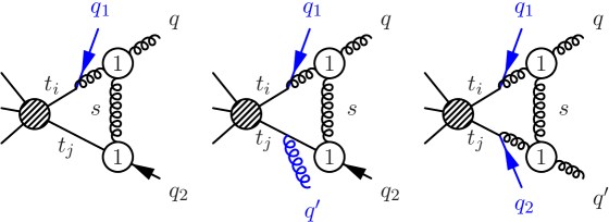
Figure 5: Relevant diagrams for the mixing $\left(J_{\chi,{\rm YM}}^{T1}\right)_{i}\left(J_{\chi,\xi}^{T1}\right)_{j}\to J^{B1}_{i}J^{A1}_{j}$ (left), $\left(J_{\chi,{\rm YM}}^{T1}\right)_{i}\left(J_{\chi,\xi}^{T1}\right)_{j}\to J^{B1}_{i}J^{B1}_{j}$ (middle) and $\left(J_{\chi,{\rm YM}}^{T1}\right)_{i}\left(J_{\chi,{\rm YM}}^{T1}\right)_{j}\to J^{B1}_{i}J^{B1}_{j}$ (right).

In order to determine the mixing into two $B$-type currents, we consider the external state $\langle f|=\langle\bar{q}_{j}g_{j}\bar{q}_{i}g_{i}|$. Restricting to gluons with $\perp$ polarization and momenta with vanishing $\perp$ component, the only possible diagram is shown in Fig. 4 (right). We find that all mixings of the type $\left(J_{\chi,\xi}^{T1}\right)_{i}\left(J_{\chi,\xi}^{T1}\right)_{j}\to J^{X1}_{i}J^{Y1}_{j}$ can be summarized as

$$\left(J_{\chi_{\alpha},\xi}^{T1}\right)_{i}\left(J_{\chi_{\beta},\xi}^{T1}\right)_{j} \to -\frac{2\alpha_{s}}{\pi\epsilon}\,G_{\lambda\kappa}^{ij}$$

$$\times\left[{\bf T}_{i}^{a}J^{A1}_{\partial^{\lambda}\chi_{\alpha}}-\frac{1}{2}\int dy\left(\gamma_{\perp i}^{\lambda}\gamma_{\perp i}^{\mu}+\frac{\gamma_{\perp i}^{\mu}\gamma_{\perp i}^{\lambda}}{\bar{y}}\right)_{\alpha\gamma}{\bf T}_{i}^{b}{\bf T}_{i}^{a}J^{B1}_{{\cal A}_{\mu}^{b}\chi_{\gamma}}(y)\right]_{i}$$

$$\times\left[{\bf T}_{j}^{a}J^{A1}_{\partial^{\kappa}\chi_{\beta}}-\frac{1}{2}\int dy^{\prime}\left(\gamma_{\perp j}^{\kappa}\gamma_{\perp j}^{\nu}+\frac{\gamma_{\perp j}^{\nu}\gamma_{\perp j}^{\kappa}}{\bar{y}^{\prime}}\right)_{\beta\delta}{\bf T}_{j}^{c}{\bf T}_{j}^{a}J^{B1}_{{\cal A}_{\nu}^{c}\chi_{\delta}}(y^{\prime})\right]_{j}\,.$$

Similarly, for time-ordered products involving ${\cal L}^{(1)}_{\rm YM}$ we find (see Fig. 5)

$$\left(J_{\chi_{\alpha},{\rm YM}}^{T1}\right)_{i}\left(J_{\chi_{\beta},\xi}^{T1}\right)_{j} \to -\frac{2\alpha_{s}}{\pi\epsilon}G_{\lambda\kappa}^{ij}$$

$$\times\,\frac{if^{bda}}{2}\int dy\,\left(\frac{2g_{\perp i}^{\mu\lambda}}{y}-\gamma_{\perp i}^{\lambda}\gamma_{\perp i}^{\mu}\right)_{\alpha\gamma}{\bf T}_{i}^{d}\left(J^{B1}_{{\cal A}_{\mu}^{b}\chi_{\gamma}}(y)\right)_{i}$$

$$\times\left[{\bf T}_{j}^{a}J^{A1}_{\partial^{\kappa}\chi_{\beta}}-\frac{1}{2}\int dy^{\prime}\left(\gamma_{\perp j}^{\kappa}\gamma_{\perp j}^{\nu}+\frac{\gamma_{\perp j}^{\nu}\gamma_{\perp j}^{\kappa}}{\bar{y}^{\prime}}\right)_{\beta\delta}{\bf T}_{j}^{c}{\bf T}_{j}^{a}J^{B1}_{{\cal A}_{\nu}^{c}\chi_{\delta}}(y^{\prime})\right]_{j}\,,$$

$$\left(J_{\chi_{\alpha},{\rm YM}}^{T1}\right)_{i}\left(J_{\chi_{\beta},{\rm YM}}^{T1}\right)_{j} \to -\frac{2\alpha_{s}}{\pi\epsilon}G_{\lambda\kappa}^{ij}$$ (3.37)

$$\times\,\frac{if^{bda}}{2}\int dy\,\left(\frac{2g_{\perp i}^{\mu\lambda}}{y}-\gamma_{\perp i}^{\lambda}\gamma_{\perp i}^{\mu}\right)_{\alpha\gamma}{\bf T}_{i}^{d}\left(J^{B1}_{{\cal A}_{\mu}^{b}\chi_{\gamma}}(y)\right)_{i}$$

$$\times\,\frac{if^{cea}}{2}\int dy^{\prime}\,\left(\frac{2g_{\perp j}^{\nu\kappa}}{y^{\prime}}-\gamma_{\perp j}^{\kappa}\gamma_{\perp j}^{\nu}\right)_{\beta\delta}{\bf T}_{j}^{e}\left(J^{B1}_{{\cal A}_{\nu}^{c}\chi_{\delta}}(y^{\prime})\right)_{j}\,.$$

The corresponding anomalous dimension matrix entries read

$$\gamma^{ij}_{\left(J_{\chi_{\alpha},\xi}^{T1}\right)_{i}\left(J_{\chi_{\beta},\xi}^{T1}\right)_{j},\left(J^{B1}_{{\cal A}_{b}^{\mu}\chi_{\gamma}}\right)_{i}\left(J^{B1}_{{\cal A}^{\nu}_{c}\chi_{\delta}}\right)_{j}}(y_{i_{1}},y_{j_{1}})$$ (3.38)

$$= \frac{\alpha_{s}}{2\pi}\,{\bf T}_{i}^{b}{\bf T}_{j}^{c}({\bf T}_{i}\cdot{\bf T}_{j})\,G_{\lambda\kappa}^{ij}\left(\gamma_{\perp i}^{\lambda}\gamma_{\perp i}^{\mu}+\frac{\gamma_{\perp i}^{\mu}\gamma_{\perp i}^{\lambda}}{\bar{y}_{i_{1}}}\right)_{\alpha\gamma}\left(\gamma_{\perp j}^{\kappa}\gamma_{\perp j}^{\nu}+\frac{\gamma_{\perp j}^{\nu}\gamma_{\perp j}^{\kappa}}{\bar{y}_{j_{1}}}\right)_{\beta\delta}\,,$$

$$\gamma^{ij}_{\left(J_{\chi_{\alpha},{\rm YM}}^{T1}\right)_{i}\left(J_{\chi_{\beta},\xi}^{T1}\right)_{j},\left(J^{B1}_{{\cal A}_{b}^{\mu}\chi_{\gamma}}\right)_{i}\left(J^{A1}_{\partial^{\nu}\chi_{\delta}}\right)_{j}}(y_{i_{1}})$$ (3.39)

$$= \frac{\alpha_{s}}{\pi}\,({\bf T}_{i}\times{\bf T}_{j})^{b}\,G_{\lambda\kappa}^{ij}\left(\frac{2g_{\perp i}^{\mu\lambda}}{y_{i_{1}}}-\gamma_{\perp i}^{\lambda}\gamma_{\perp i}^{\mu}\right)_{\alpha\gamma}g^{\kappa\nu}\delta_{\beta\delta}\,,$$

$$\gamma^{ij}_{\left(J_{\chi_{\alpha},{\rm YM}}^{T1}\right)_{i}\left(J_{\chi_{\beta},\xi}^{T1}\right)_{j},\left(J^{B1}_{{\cal A}_{b}^{\mu}\chi_{\gamma}}\right)_{i}\left(J^{B1}_{{\cal A}^{\nu}_{c}\chi_{\delta}}\right)_{j}}(y_{i_{1}},y_{j_{1}})$$ (3.40)

$$= -\frac{\alpha_{s}}{2\pi}\,{\bf T}_{j}^{c}({\bf T}_{i}\times{\bf T}_{j})^{b}\,G_{\lambda\kappa}^{ij}\left(\frac{2g_{\perp i}^{\mu\lambda}}{y_{i_{1}}}-\gamma_{\perp i}^{\lambda}\gamma_{\perp i}^{\mu}\right)_{\alpha\gamma}\left(\gamma_{\perp j}^{\kappa}\gamma_{\perp j}^{\nu}+\frac{\gamma_{\perp j}^{\nu}\gamma_{\perp j}^{\kappa}}{\bar{y}_{j_{1}}}\right)_{\beta\delta}\,,$$

$$\gamma^{ij}_{\left(J_{\chi_{\alpha},{\rm YM}}^{T1}\right)_{i}\left(J_{\chi_{\beta},{\rm YM}}^{T1}\right)_{j},\left(J^{B1}_{{\cal A}_{b}^{\mu}\chi_{\gamma}}\right)_{i}\left(J^{B1}_{{\cal A}^{\nu}_{c}\chi_{\delta}}\right)_{j}}(y_{i_{1}},y_{j_{1}})$$ (3.41)

$$= -\frac{\alpha_{s}}{2\pi}\,f^{bda}f^{cea}\,{\bf T}_{i}^{d}{\bf T}_{j}^{e}\,G_{\lambda\kappa}^{ij}\left(\frac{2g_{\perp i}^{\mu\lambda}}{y_{i_{1}}}-\gamma_{\perp i}^{\lambda}\gamma_{\perp i}^{\mu}\right)_{\alpha\gamma}\!\left(\frac{2g_{\perp j}^{\nu\kappa}}{y_{j_{1}}}-\gamma_{\perp j}^{\kappa}\gamma_{\perp j}^{\nu}\right)_{\beta\delta}\,.$$

Here we defined the colour operator cross product via $({\bf T}_{i_{1}}\times{\bf T}_{i_{2}})^{a}\equiv if^{abc}{\bf T}_{i_{1}}^{b}{\bf T}_{i_{2}}^{c}$.

3.3 Single insertion of ${\cal L}^{(2)}$

Figure 6: As Fig. 2, but for an insertion of ${\cal L}^{(2)}_{\xi}$ or ${\cal L}^{(2)}_{\rm YM}$. The relevant diagrams are obtained by choosing up to two emissions. Dashed lines should be replaced with subdiagrams according to the lower panel of Fig. 2. In addition, also emission directly off the current is possible.

In this section we consider the possible mixing of single insertions of ${\cal O}(\lambda^{2})$ SCET interactions, that is, $J^{T2}_{\chi,V}$, into current operators. It is sufficient to take $V=\xi,{\rm YM}$, because at ${\cal O}(\lambda^{2})$, the time-ordered product $J^{T2}_{\chi,\xi q}$ cannot mix into currents. The reason is that for diagrams with only collinear external lines, the soft quark field from ${\cal L}^{(2)}_{\xi q}$ would have to be contracted with another subleading-power Lagrangian.

The class of one-loop diagrams to be considered is illustrated exemplarily in Fig. 6, where the dashed lines represent again possible additional collinear emissions. To capture all possible mixings into currents at ${\cal O}(\lambda^{2})$ we need to consider up to two additional collinear emissions.

We begin with the case of no extra collinear emission off the power-suppressed vertex from the ${\cal L}_{\xi}^{(2)}$ insertion (in direction $i$). The soft loop momentum $l$ carried by the soft gluon propagator is assumed to flow outwards of the ${\cal L}_{\xi}^{(2)}$-vertex, and the single external collinear momentum in the $i$ direction is denoted by $p$. Furthermore, we assume that the internal collinear line attached to the ${\cal L}_{\xi}^{(2)}$-vertex has momentum $\tilde{p}-l$, and we keep $\tilde{p}\not=p$ until derivatives are taken. The loop amplitude can then be written as

$$\langle f|\chi_{i}\chi_{j}|0\rangle_{{\rm single}\ {\cal L}^{(2)}_{\xi}\ {\rm insertion}} = \tilde{\mu}^{2\epsilon}\int_{l}\bigg{(}S^{\rho\nu}(-l,-p,\tilde{p}+l)\,{\cal A}_{i}^{a}\,(-l_{\rho}g_{\nu\mu}+l_{\nu}g_{\rho\mu})\bigg{)}_{i}\bigg{|}_{\tilde{p}=p}$$ (3.42)

$$\times\frac{-ig_{\mu\mu^{\prime}}}{l^{2}+i\varepsilon}\times\Big{(}n_{j-}^{\mu^{\prime}}{\cal A}_{j}^{a}\Big{)}_{j}$$

where $S^{\rho\nu}$ is given by Eq. (A.33) and arises from the ${\cal L}_{\xi}^{(2)}$ insertion. As before, ${\cal A}_{i}^{a}$ (${\cal A}_{j}^{a}$) contains the part of the amplitude involving $i$-collinear ($j$-collinear) propagators, vertices, polarization vectors and external spinors, and $a$ denotes the colour index of the soft gluon. We suppress Dirac indices for brevity. For the diagram without any extra emissions, $q_{1}\equiv p$, $\tilde{q}_{1}=\tilde{p}-l$,

$${\cal A}_{i}^{a}\Big{|}_{\rm no\ extra\ emission} = \frac{-in_{i+}\tilde{q}_{1}}{\tilde{q}_{1}^{2}+n_{i+}\tilde{q}_{1}n_{i-}l}ig_{s}t^{a}v_{i}(q_{1})\,,$$ (3.43)

and ${\cal A}_{j}^{a}$ is given by Eq. (3.14).

In general ${\cal A}_{i}^{a}$ and ${\cal A}_{j}^{a}$ contain several propagators involving various combinations of external momenta, and vertex factors that may depend polynomially on $n_{i-}l$ and $n_{j-}l$, respectively. By partial fractioning the integrand ${\cal A}_{i}$ can be brought into the generic form

$${\cal A}_{i}^{a}=\sum_{p_{i},a_{i},b_{i}}C^{a}(p_{i};a_{i},b_{i})\,(n_{i-}l)^{b_{i}}\left(\frac{n_{i+}p_{i}}{p_{i}^{2}+n_{i+}p_{i}n_{i-}l}\right)^{a_{i}}$$ (3.44)

where $p_{i}$ are (linear combinations of) collinear momenta in direction $i$, including $p$ and $\tilde{p}$. We also use $p_{i}$ in the above equation to label the sum of terms that arises from the partial fractioning. The coefficients $C^{a}(p_{i};a_{i},b_{i})$ may depend on the collinear momenta $p_{i}$, but not on $l$. ${\cal A}_{j}^{a}$ can be decomposed analogously. From the explicit form of $S^{\rho\nu}$ together with Eqs. (3.7) and (3.15) we obtain

$$\langle f|\chi_{i\alpha}\chi_{j\beta}|0\rangle_{{\rm single}\ {\cal L}^{(2)}_{\xi}\ {\rm insertion}}$$ (3.45)

$$= -i\tilde{\mu}^{2\epsilon}\int_{l}\,\left[\left(\frac{\partial}{\partial n_{i+}\tilde{p}}-\frac{1}{d-2}\frac{\partial}{\partial\tilde{p}_{\perp i}}\cdot\frac{\partial}{\partial\tilde{p}_{\perp i}}n_{i-}l\right){\cal A}_{i}^{a}\right]_{\tilde{p}=p}\times\frac{n_{j-}l}{l^{2}}{\cal A}_{j}^{a}\,.$$

After inserting Eq. (3.44), the loop integral takes the form of the master integral (B.3). A peculiar property of this integral is that it factors into two terms, each of which depends only on quantities related to a single collinear direction, here $i$ and $j$. This property is manifest in a frame where directions $i$ and $j$ are back-to-back. In the back-to-back frame, the $l_{\perp}$ integral can be performed first and the resulting expression is a product of two integrals that depend only on $n_{-}l$ or on $n_{+}l$. Such a boost to the back-to-back frame can always be performed. Hence, the soft loop diagram factorizes into

$$\langle f|\chi_{i}\chi_{j}|0\rangle_{{\rm single}\ {\cal L}^{(2)}_{\xi}\ {\rm insertion}}=-F_{\epsilon}\times{\cal D}_{i}^{a}\times{\cal D}_{j}^{a}$$ (3.46)

with $F_{\epsilon}$ given by Eq. (B), and

$${\cal D}_{i}^{a} = \sum_{p_{i}a_{i}b_{i}}\bigg{(}D(a_{i},b_{i},\epsilon)\frac{\partial}{\partial n_{i+}\tilde{p}}$$ (3.47)

$${}+\frac{D(a_{i},b_{i}+1,\epsilon)}{2-2\epsilon}\frac{\partial}{\partial\tilde{p}_{\perp i}}\cdot\frac{\partial}{\partial\tilde{p}_{\perp i}}\frac{p_{i}^{2}}{n_{i+}p_{i}}\bigg{)}\frac{C^{a}(p_{i};a_{i},b_{i})}{(p_{i}^{2}/n_{i+}p_{i})^{a_{i}-b_{i}-1+\epsilon}}\bigg{|}_{\tilde{p}=p},$$

where the numerical coefficients $D(a,b,\epsilon)$ are defined in Eq. (B.4), and

$${\cal D}_{j}^{a} = -\sum_{p_{j},a_{j},b_{j}}\frac{C^{a}(p_{j};a_{j},b_{j})D(a_{j},b_{j}+1,\epsilon)}{(p_{j}^{2}/n_{j+}p_{j})^{a_{j}-b_{j}-2+\epsilon}}\,.$$ (3.48)

The diagrams with extra emission off the subleading-power vertex can be treated analogously, and lead to an integral of similar form, proportional to the same factor ${\cal D}_{j}^{a}$. Similarly, diagrams involving an insertion of ${\cal L}_{\rm YM}^{(2)}$ in the $i$ direction can be shown to factorize into a product involving the same ${\cal D}_{j}^{a}$. This is a consequence of the fact that the $j$-direction involves only leading-power soft interactions, which are of eikonal type, and hence identical for quarks and gluons except for the colour factor. From the following discussion it will become clear that this is the relevant property.

No extra emissions in direction $j$:

In this case the amplitude $\mathcal{A}^{a}_{j}$ is given by Eq. (3.14). There is only a single collinear propagator with $p_{j}=q_{2}$, $a_{j}=1$, $b_{j}=0$, $C^{a}(p_{j};a_{j},b_{j})=g_{s}t^{a}$ (where $a$ is the colour index of the soft gluon), $D(1,1,\epsilon)=-1$, which gives

$$({\cal D}_{j}^{a})_{{\rm no\,}j-{\rm coll.\,em.}}=g_{s}t^{a}\mu^{\epsilon}\left(\frac{q_{2}^{2}}{n_{j+}q_{2}}\right)^{1-\epsilon}\,.$$ (3.49)

Hence, the factor ${\cal D}_{j}^{a}$ vanishes when the off-shell infrared regulator is removed, $q_{2}^{2}\to 0$. Due to integral factorization ${\cal D}_{i}$ cannot depend on the $j$-collinear momentum $q_{2}$, and therefore the complete diagram vanishes in this limit. Together with the factorization property, this finding also proves that all diagrams with extra collinear emissions in direction $i$, but no emissions in direction $j$, vanish, because they are all proportional to $({\cal D}_{j}^{a})_{{\rm no\,}j-{\rm coll.\,em.}}$.

Single extra emission in direction $j$:

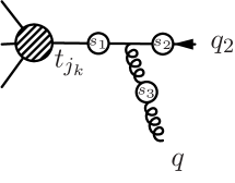
Figure 7: Diagram with a single collinear emission in direction $j$. The insertions $s_{k}$ show possible attachments of the soft line. The part of the diagram in direction $i$ is not shown.

The factorization property (3.46) extends to the sum of all diagrams with soft attachments to a given collinear splitting pattern in direction $j$. This can be captured by the expression ${\cal D}_{j}^{a}$ from Eq. (3.48) by including in the sum on the right-hand side the sum over all soft attachments. In the following, it turns out to be sufficient to consider only the $j$-collinear direction, which contains the leading-power soft interactions.

To be specific, consider a collinear quark in direction $j$ with external momentum $q_{2}$, and an emission of a collinear gluon off the quark line (momentum $q$, colour $b$, polarization tensor $\epsilon$), as shown in Fig. 7. The part of the diagram along direction $i$, which involves the ${\cal L}_{\xi}^{(2)}$ insertion, is not shown, because it is irrelevant for the computation of ${\cal D}_{j}^{a}$ due to the factorization property. The insertions $s_{k}$ mark attachments of the soft gluon (momentum $l$, colour $a$) to either the internal quark propagator ($s_{1}$), the external quark ($s_{2}$) or the gluon ($s_{3}$). The corresponding amplitudes are given by

$${\cal A}_{j}^{a(s_{1})} = \frac{-in_{j+}\hat{q}}{\hat{q}^{2}-n_{j+}\hat{q}n_{j-}l}\,ig_{s}t^{a}\frac{-in_{j+}\hat{q}}{\hat{q}^{2}}\,ig_{s}t^{b}C_{j}v_{j}(q_{2})\,,$$

$${\cal A}_{j}^{a(s_{2})} = \frac{-in_{j+}\hat{q}}{\hat{q}^{2}-n_{j+}\hat{q}n_{j-}l}\,ig_{s}t^{b}C_{j}\frac{-in_{j+}q_{2}}{q_{2}^{2}-n_{j+}q_{2}n_{j-}l}\,ig_{s}t^{a}v_{j}(q_{2})\,,$$

$${\cal A}_{j}^{a(s_{3})} = \frac{-in_{j+}\hat{q}}{\hat{q}^{2}-n_{j+}\hat{q}n_{j-}l}\,ig_{s}t^{c}C_{j}v_{j}(q_{2})\,(-g_{s}f^{abc}n_{j+}q)\frac{-i}{q^{2}-n_{j+}qn_{j-}l}\,,$$ (3.50)

where $\hat{q}\equiv q_{2}+q$, and

$$C_{j}\equiv\frac{\not{\hat{q}}_{\perp j}\not{\epsilon}_{\perp j}}{n_{j+}\hat{q}}+\frac{\not{\epsilon}_{\perp j}\not{q}_{2\perp j}}{n_{j+}q_{2}}\,.$$ (3.51)

We have used that the three-gluon vertex involving two collinear and one soft gluon is diagonal in the Lorentz indices of the collinear fields. The factor $n_{j-}^{\mu}$ that is contained in the soft leading-power vertex is not part of the above amplitudes, since it was taken out in the defining Eq. (3.42). The sum of the three amplitudes can be expanded using partial fractioning as (we omit the label for $a_{j}=1,b_{j}=0$ on the $C^{a}$ coefficients common to all terms for brevity in the following equation)

$$\sum_{k=1}^{3}{\cal A}_{j}^{a(s_{k})}=C^{a}(\hat{q})\frac{n_{j+}\hat{q}}{\hat{q}^{2}-n_{j+}\hat{q}n_{j-}l}+C^{a}(q_{2})\frac{n_{j+}q_{2}}{q_{2}^{2}-n_{j+}q_{2}n_{j-}l}+C^{a}(q)\frac{n_{j+}q}{q^{2}-n_{j+}qn_{j-}l}\,,$$ (3.52)

with coefficients

$$C^{a}(\hat{q}) = g_{s}^{2}\bigg{(}t^{a}t^{b}\frac{n_{j+}\hat{q}}{\hat{q}^{2}}+t^{b}t^{a}\Delta_{q_{2}\hat{q}}+if^{abc}t^{c}\Delta_{q\hat{q}}\bigg{)}C_{j}v_{j}(q_{2})\,,$$

$$C^{a}(q_{2}) = g_{s}^{2}t^{b}t^{a}\Delta_{\hat{q}q_{2}}C_{j}v_{j}(q_{2})\,,$$

$$C^{a}(q) = g_{s}^{2}if^{abc}t^{c}\Delta_{\hat{q}q}C_{j}v_{j}(q_{2})\,,$$ (3.53)

and

$$\Delta_{qp}\equiv\left(\frac{q^{2}}{n_{j+}q}-\frac{p^{2}}{n_{j+}p}\right)^{\!-1}=-\Delta_{pq}\,.$$ (3.54)

Using Eq. (3.48) with $a_{j}=1$, $b_{j}=0$, this gives

$$({\cal D}_{j}^{a})_{{\rm single\,}j-{\rm coll.\,em.}} = \Bigg{\{}C^{a}(\hat{q})\left(\frac{\hat{q}^{2}}{n_{j+}\hat{q}}\right)^{1-\epsilon}+C^{a}(q_{2})\left(\frac{q_{2}^{2}}{n_{j+}q_{2}}\right)^{1-\epsilon}+C^{a}(q)\left(\frac{q^{2}}{n_{j+}q}\right)^{1-\epsilon}\Bigg{\}}$$ (3.55)

$$= g_{s}^{2}\mu^{\epsilon}\Bigg{\{}t^{a}t^{b}\left(\frac{\hat{q}^{2}}{n_{j+}\hat{q}}\right)^{-\epsilon}+t^{b}t^{a}\Delta_{q_{2}\hat{q}}\left(\left(\frac{\hat{q}^{2}}{n_{j+}\hat{q}}\right)^{1-\epsilon}-\left(\frac{q_{2}^{2}}{n_{j+}q_{2}}\right)^{1-\epsilon}\right)$$

$${}+if^{abc}t^{c}\Delta_{q\hat{q}}\left(\left(\frac{\hat{q}^{2}}{n_{j+}\hat{q}}\right)^{1-\epsilon}-\left(\frac{q^{2}}{n_{j+}q}\right)^{1-\epsilon}\right)\Bigg{\}}\,C_{j}u_{j}(q_{2})$$

$$= g_{s}^{2}\left\{t^{a}t^{b}-t^{b}t^{a}-if^{abc}t^{c}\right\}\left(\frac{\hat{q}^{2}}{n_{j+}\hat{q}}\right)^{-\epsilon}C_{j}u_{j}(q_{2})+{\cal O}(q^{2},q_{2}^{2})$$

$$= {\cal O}(q^{2},q_{2}^{2})\,,$$

where in the last two lines we have expanded in the small off-shell regulators $q_{2}^{2}$ and $q^{2}$ of the external quark and gluon, respectively. Therefore, in the on-shell limit $q^{2},q_{2}^{2}\to 0$ when the regulators are removed, also all contributions with a single emission in direction $j$ vanish.

This result is not unexpected: It is well known that in the eikonal limit the coupling of a soft gluon to a pair of partons from collinear splitting is equal to the coupling to the parent parton. The above considerations proves that this holds true when the amplitude is first regulated by a small off-shellness, which is then removed. In the SCET framework the standard eikonal cancellation in the absence of the off-shell regulator is reflected in the decoupling transformation [25], which removes soft-gluon interactions from the leading-power Lagrangian. In the on-shell limit, the soft interaction is then described by a soft Wilson line evaluated at the position of the current (which we choose to be $x=0$). This gives

$${\cal A}^{a}_{j}=\sum_{k=1}^{3}{\cal A}^{a(s_{k})}_{j}=-\frac{g_{s}t^{a}}{n_{j-}l}\times\frac{-in_{j+}\hat{q}}{\hat{q}^{2}}\,ig_{s}C_{j}v_{j}(q_{2})\,,$$

which is the product of the Wilson line (eikonal) factor and the collinear splitting amplitude. Together with the explicit factor $n_{j-}l$ in the numerator in Eq. (3.45) this implies that the loop integral does not depend on the $n_{j-}$ direction, and therefore vanishes. The above shows that in the present case the naive argument based on unregulated on-shell amplitudes remains valid as the limiting case of an off-shell regulated amplitude.

Double extra emission in direction $j$:

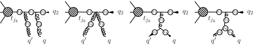
Figure 8: Diagrams with double collinear emission in direction $j$. The insertions $s_{k}$ show possible attachments of the soft line. The part of the diagram in direction $i$ is not shown. Also the crossed diagram corresponding to the first one with momenta $q$ and $q^{\prime}$ interchanged in not shown.

The diagrams in Fig. 8 show collinear splittings in the $j$ direction involving two extra emissions, and possible positions $s_{k}$ for attachment of the soft line in each case. One needs to sum up the amplitudes ${\cal A}_{j}^{a(s_{k})}$ for all $s_{k}$. For each of the four classes of diagrams that are indicated in the figure, we find that, following the same steps as above, the ${\cal D}_{j}^{a}$ part of the soft loop amplitude vanishes when the off-shell regulators are removed. Once again, this is a consequence of the SCET version of the leading-power eikonal-type couplings of soft gluons to collinear lines. Thus,

$$({\cal D}_{j}^{a})_{{\rm double\,}j-{\rm coll.\,em.}} = {\cal O}(q_{2}^{2},q^{2},{q^{\prime}}^{2})$$ (3.56)

Altogether, this implies that the time-ordered products $J^{T2}_{\chi,V}$ do not mix into current operators, i.e.

$$\gamma^{ij}_{T(P,{\cal L}_{k}^{(2)}),Q}=0\,,$$ (3.57)

where $i,j,k=1,\dots,N$ and $P,Q$ are $N$-jet current operators with fermion number one.

3.4 Soft-quark exchange

For the mixed cases $(F_{i},F_{j})=(+1,-1)$ and $(F_{i},F_{j})=(-1,+1)$, an additional class of diagrams with soft-quark exchange from two ${\cal L}_{\xi q}^{(1)}$ insertions exists. An example is shown in Fig. 9. We show that these diagrams vanish, if the mass of the soft quark can be neglected.

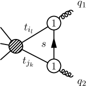
Figure 9: Example for a soft fermion exchange one-loop diagram.

Even for an arbitrary number of collinear emissions attached to any internal or external propagator, or vertex, the soft loop momentum $l$ enters the integral only via $n_{i-}l$ and $n_{j-}l$, except for the soft (massless) quark propagator $\not{l}/l^{2}$. This gives a loop integral of the form

$${\cal I}_{\xi q}=-i\tilde{\mu}^{2\epsilon}\int\frac{d^{d}l}{(2\pi)^{d}}\,\not{l}F(n_{i-}l,n_{j-}l,l^{2})=C_{1}\not{n}_{i-}+C_{2}\not{n}_{j-}\,,$$ (3.58)

with some function $F$ and coefficients $C_{k}$. The vertex from ${\cal L}_{\xi q}^{(1)}$ contracts the soft quark propagator indices with collinear quarks. Therefore we may insert a collinear projector with respect to $i$ and $j$ to the left and to the right, respectively. This results in

$$\frac{\not{n}_{i+}\not{n}_{i-}}{4}{\cal I}_{\xi q}\frac{\not{n}_{j-}\not{n}_{j+}}{4}=\frac{\not{n}_{i+}\not{n}_{i-}}{4}(C_{1}\not{n}_{i-}+C_{2}\not{n}_{j-})\frac{\not{n}_{j-}\not{n}_{j+}}{4}=0\,.$$ (3.59)

Therefore, generally, there is no one-loop soft-quark exchange mixing

$$J^{T1}_{\psi,\xi q}J^{T1}_{\psi^{\prime},\xi q}\to 0\,,$$ (3.60)

for $\psi,\psi^{\prime}=\chi,\bar{\chi},{\cal A}$. Since operators involving only a single ${\cal L}_{\xi q}^{(1)}$ insertion vanish trivially (the soft quark cannot be connected to different collinear directions at leading power), this generalizes to

$$J^{T1}_{\psi,\xi q}J^{X1}\to 0\,,$$ (3.61)

where $J^{X1}$ can be an arbitrary ${\cal O}(\lambda)$ current or time-ordered product. This can be summarized by

$$\gamma^{ij}_{T(P,{\cal L}^{(1)}_{k,\xi q}),Q}=\gamma^{ij}_{T(P,{\cal L}^{(1)}_{k,\xi q},{\cal L}^{(1)}_{l,\xi q}),Q}=0\,,$$ (3.62)

for $i,j,k,l=1,\dots,N$ and arbitrary current operators $P,Q$. The absence of diagrams with a soft quark line implies that fermion number is conserved in each collinear sector separately up to one-loop and $\mathcal{O}\left(\lambda^{2}\right)$, which allows us to classify the next-to-leading power anomalous dimension according to collinear sectors with definite fermion number.

The vanishing of mixing from soft-quark exchange holds only for massless fermions as assumed throughout this paper. As an aside, we note that when the fermion mass $m$ is parametrically of order of the soft scale, $\not{l}\to\not{l}+m$ in Eq. (3.58), which adds a term $C_{3}m$ to the right-hand side of this equation. This term is not projected to zero in Eq. (3.59). An explicit example of the relevance of soft-fermion exchange can be found in Ref. [26], where it contributes to the leading logarithm of a power-enhanced electromagnetic effect in the rare $B$-meson decay $B_{s}\to\ell^{+}\ell^{-}$. Technically, the basis of ${\cal O}(\lambda^{2})$ suppressed operators must be extended by mass-suppressed operators $J_{i}^{A2}=mJ^{A0}_{i}$, and the non-zero mixing is of the form

$$J^{T1}_{\psi_{i},\xi q}J^{T1}_{\psi_{j}^{\prime},\xi q}\to mJ^{A0}_{i}J^{A0}_{j}\,.$$ (3.63)

4 Collinear sector

In the collinear sector it is sufficient to consider a single collinear direction, say $i$, since collinear fields corresponding to different directions do not interact with each other. We categorize different cases by their fermion number $F_{i}$ and power suppression $\lambda^{n}$. Results for $F_{i}=-1$ can be obtained from $F_{i}=+1$ by hermitian conjugation (see App. D for details). The case $F_{i}=2$ was treated in Ref. [14]. Note that $|F_{i}|\leq n+1$ since each additional fermionic building block costs a power of $\lambda$ relative to the leading power. In the following we consider the cases $F_{i}=1$ and $F_{i}=3$. Since the time-ordered product operators inherit their collinear anomalous dimension from the current operators, see Eq. (2.21), we give only the current-current part of the anomalous dimension matrix $\gamma^{i}_{PQ}$.

4.1 ${\mathcal{O}(\lambda)}$

At ${\cal O}(\lambda)$ $F_{i}=3$ is not possible. For $F_{i}=1$ we find for the collinear anomalous dimension $\gamma^{i}_{PQ}$ in Eq. (2.17),

$$\gamma^{i}_{PQ}\quad=\quad\begin{array}[]{c||c|c}&J^{A1}_{\partial\chi}&J^{B1}_{{\cal A}\chi}\\ \hline\cr\hline\cr J^{A1}_{\partial\chi}&0&0\\ \hline\cr J^{B1}_{{\cal A}\chi}&0&\gamma^{i}_{{\cal A}\chi,{\cal A}\chi}\\ \end{array}$$ (4.1)

where the non-zero entry is given in App. C of Ref. [14]. The $A$-type operator $J^{A1}_{\partial\chi}$ has matrix elements identical to the leading power operator $J^{A0}_{\chi}$, up to overall factors of external momenta due to the total derivative. This implies $\gamma^{i}_{J^{A1}J^{B1}}=0$. The diagonal anomalous dimension of $J^{A1}_{\partial\chi}$ is already accounted for by the first line of Eq. (2.17), and therefore also $\gamma^{i}_{J^{A1}J^{A1}}=0$. To show $\gamma^{i}_{J^{B1}J^{A1}}=0$ we compute the matrix element of $J^{B1}_{{\cal A}\chi}$ for an external state with a single fermion, and find that it vanishes.

4.2 ${\mathcal{O}(\lambda^{2})}$, overview

At ${\cal O}(\lambda^{2})$, we find for $F_{i}=1$

$$\gamma^{i}_{PQ}\quad=\quad\begin{array}[]{c||c|cc|ccc}&J^{A2}_{\partial\partial\chi}&J^{B2}_{{\cal A}\partial\chi}&J^{B2}_{\partial({\cal A}\chi)}&J^{C2}_{{\cal AA}\chi}&J^{C2}_{\chi\bar{\chi}\chi}\\ \hline\cr\hline\cr J^{A2}_{\partial\partial\chi}&0&0&0&0&0\\ \hline\cr J^{B2}_{{\cal A}\partial\chi}&0&\eqref{eq:gamma_Adelchi_Adelchi}&\eqref{eq:gamma_Adelchi_delAchi}&\eqref{eq:gamma_Adelchi_AAchi}&\eqref{eq:gamma_Adelchi_chichibarchi}\\ J^{B2}_{\partial({\cal A}\chi)}&0&0&\eqref{eq:gamma_delAchi_delAchi}&0&0\\ \hline\cr J^{C2}_{{\cal AA}\chi}&0&0&0&\eqref{eq:gamma_AAchi_AAchi}&\eqref{eq:gamma_AAchi_chichibarchi}\\ J^{C2}_{\chi\bar{\chi}\chi}&0&0&0&\eqref{eq:gamma_chichibarchi_AAchi}&\eqref{eq:gamma_chichibarchi_chichibarchi}\\ \end{array}$$ (4.8)

The first row vanishes, which follows from an argument analogous to the ${\cal O}(\lambda)$ case. The non-zero entries of $\gamma^{i}_{PQ}$ point to the equation numbers of the corresponding results given below. They can be divided into three cases: first, mixing of $B$-type currents into $B$-type currents (middle block); second, mixing of $B$-type currents into $C$-type currents (last two columns of second row); and third, mixing of $C$-type currents into $C$-type currents (lower right block). In the following we discuss these three cases in turn, see Secs. 4.3 to 4.5.

Let us briefly comment on the remaining zero entries. For the first column, second row, we compute a matrix element of $J^{B2}_{{\cal A}\partial\chi}$ with a single fermion of momentum $p$ and find that the result is proportional to the off-shell regulator $p^{2}$. This implies that the corresponding anomalous dimension vanishes in the on-shell limit. The renormalization of $J^{B2}_{\partial({\cal A}\chi)}$ is identical to $J^{B1}_{{\cal A}\chi}$ at ${\cal O}(\lambda)$ due to the total derivative, which implies the zero entries in the third row. Finally, as will be discussed in Sec. 4.5, at the one-loop order considered here, the renormalization of $C$-type currents can be related to the one of $B$-type currents at ${\cal O}(\lambda)$. From Eq. (4.1) together with corresponding results found in Ref. [14] this implies the zero entries in the last two rows.

For $F_{i}=3$ only the single operator $J^{C2}_{\chi\chi\chi}$ exists at ${\cal O}(\lambda^{2})$. The corresponding anomalous dimension is given in Sec. 4.5, see Eq. (4.42).

Before turning to the explicit computation, we comment on the mixing into operators with gluon building blocks, which requires the calculation of matrix element with external gluons. We implement the transversality condition $\epsilon\cdot q=0$ of the polarization vector of a gluon with momentum $q$ by eliminating $n_{i-}\epsilon$ through the identity

$$n_{i-}\epsilon=-\frac{n_{i+}\epsilon n_{i-}q+2\epsilon_{\perp i}\cdot q_{\perp i}}{n_{i+}q}\,.$$ (4.9)

This is consistent with the fact that we do not consider operators containing the building block $n_{i-}{\cal A}$, which can be eliminated by an equation-of-motion identity [14]. In practice, the above equation can be simplified. Knowing that $n_{i+}A$ appears only within collinear Wilson lines, it is never necessary to consider diagrams with external $n_{i+}A$ gluons, hence we can replace

$$n_{i-}\cdot\epsilon\to-\frac{2\epsilon_{\perp i}\cdot q_{\perp i}}{n_{i+}q}\,.$$ (4.10)

Whenever the operator under consideration does not contain transverse derivatives, the external transverse momentum $q_{\perp i}$ may be set to zero, in which case the calculation can be performed from the beginning assuming $n_{i\pm}\cdot\epsilon=0$.

4.3 Mixing of $B$-type currents into $B$-type currents

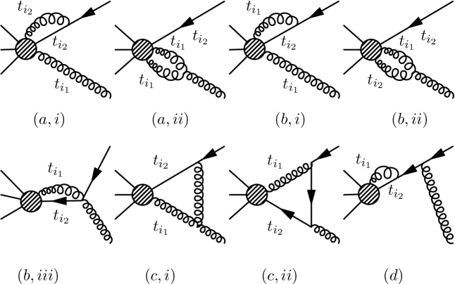
Figure 10: Diagrams contributing to the mixing of $B$-type currents into $B$-type currents in the collinear sector with fermion number $F_{i}=1$.

We start with the second row of Eq. (4.8), i.e. the entry for $J^{B2}_{{\cal A}\partial\chi}(x)\to J^{B2}_{{\cal A}\partial\chi}(y)$ and the mixing $J^{B2}_{{\cal A}\partial\chi}(x)\to J^{B2}_{\partial({\cal A}\chi)}(y)$. $B$-type currents depend only on a single independent collinear momentum fraction, which we denote by $x\equiv x_{i_{1}}$ ($y\equiv y_{i_{1}}$ for the operator mixed into.) The momentum fraction carried by the second (in the present case, fermion) building block is $\bar{x}=1-x$ and $\bar{y}=1-y$, respectively. In order to extract the anomalous dimension, we consider a matrix element of $J^{B2}_{{\cal A}\partial\chi}$ with an outgoing antiquark and a gluon. The corresponding collinear one-loop diagrams are shown in Fig. 10. In our convention, $F_{i}=+1$ corresponds to fermion flow directed towards the current, as indicated by the arrows. As discussed above, we assume that the polarization vector for the external gluon satisfies $n_{i+}\epsilon=0$, and replace $n_{i-}\epsilon$ according to Eq. (4.10).

The diagrams can be classified as in Ref. [14]. Loops involving only internal lines attached to a single collinear building block ($(a,i)$ and $(a,ii)$ in Fig. 10) are responsible for the contributions to $\delta Z_{PQ}^{c,i}(x,y)$ with $k=l$ in Eq. (2.15), that encompass a double pole $1/\epsilon^{2}$ and are diagonal with respect to collinear momentum fractions $x$ and $y$. They do not contribute to the part $\gamma^{i}_{PQ}$ that is off-diagonal with respect to the momentum fractions, and proportional to a single power of $1/\epsilon$. For completeness we report the result for the sum of diagrams $(a,i)$ and $(a,ii)$, added to the tree-level result, and adding also the contributions from the right-hand side of the renormalization condition (2.2) that involves field renormalization factors. We denote this particular sum of terms by the subscript $(a)$,

$$\langle\bar{q}(p)g(q)|J^{B2}_{{\cal A}\partial\chi}(x)|0\rangle_{(a)}=J_{q}(p^{2})J_{g}(q^{2})\int dy\delta(x-y)\langle\bar{q}(p)\bar{g}(q)|J^{B2}_{{\cal A}\partial\chi}(y)|0\rangle_{\rm tree}\,,$$ (4.11)

where

$$J_{q}(p^{2}) = 1+\frac{\alpha_{s}C_{F}}{4\pi}\left[\frac{2}{\epsilon^{2}}+\frac{2}{\epsilon}\ln\left(\frac{\mu^{2}}{-p^{2}}\right)+\frac{3}{2\epsilon}\right]+{\cal O}(\epsilon^{0})\,,$$

$$J_{g}(q^{2}) = 1+\frac{\alpha_{s}C_{A}}{4\pi}\left[\frac{2}{\epsilon^{2}}+\frac{2}{\epsilon}\ln\left(\frac{\mu^{2}}{-q^{2}}\right)\right]+{\cal O}(\epsilon^{0})$$ (4.12)

coincide with the leading-power collinear contributions from a single fermionic or gluonic building block [2, 27]. We also introduced an integration over $y$ in order to stress that contributions from $(a,i)$, $(a,ii)$ and field renormalization are diagonal with respect to the momentum fractions.

Loops involving internal lines that are attached to the two different building blocks may change momentum fractions and therefore contribute to $\gamma^{i}_{PQ}$. In addition, $(b,i)$ and $(b,ii)$ in Fig. 10 also yield diagonal contributions proportional to $\delta(x-y)$ that provide the terms with $k\not=l$ in (2.15). At ${\cal O}(\lambda^{2})$, as considered here, the one-particle reducible (1PR) diagram $(d)$ needs to be taken into account. The loop itself is proportional to the sum of all external momenta squared, which cancels the 1PR propagator, and yields a non-zero contribution.

Adding all contributions, we find for $J^{B2}_{{\cal A}\partial\chi}\to J^{B2}_{{\cal A}\partial\chi}$ (all results for collinear contributions $\gamma^{i}_{PQ}$ refer to collinear direction $i$; we omit the label $i$ of the corresponding light-cone basis vectors and $\perp$ projections for brevity here and below)

$$\gamma^{i}_{{\cal A}^{\mu}\partial^{\nu}\chi,{\cal A}^{\rho}\partial^{\sigma}\chi}(x,y) = {}g_{\perp}^{\mu\rho}g_{\perp}^{\nu\sigma}\frac{\alpha_{s}{\bf T}_{i_{1}}\cdot{\bf T}_{i_{2}}}{2\pi}\Bigg{\{}\theta(x-y)\left[\frac{1}{x-y}\right]_{+}+\theta(y-x)\left[\frac{1}{y-x}\right]_{+}$$ (4.13)

$${}-\theta(x-y)\frac{\bar{x}+\bar{y}}{\bar{y}^{2}}-\theta(y-x)\frac{x+2y}{2y^{2}}\Bigg{\}}$$

$${}+\frac{\alpha_{s}{\bf T}_{i_{1}}\cdot{\bf T}_{i_{2}}}{8\pi}M^{\mu\nu,\rho\sigma}(x,y)-\frac{\alpha_{s}({\bf C_{F}}+{\bf T}_{i_{1}}\cdot{\bf T}_{i_{2}})}{8\pi}N^{\mu\nu,\rho\sigma}(x,y)$$

$${}+\frac{\alpha_{s}{\bf C_{F}}}{8\pi}\frac{\bar{x}}{\bar{y}}(2g_{\perp}^{\mu\nu}-x\gamma_{\perp}^{\mu}\gamma_{\perp}^{\nu})\left(\gamma_{\perp}^{\rho}\gamma_{\perp}^{\sigma}+\frac{2\bar{y}}{y}g_{\perp}^{\rho\sigma}\right)\,,$$

where, in colour operator notation, ${\bf C_{F}}\equiv\frac{1}{6}(1-3({\bf T}_{i_{1}}+{\bf D}_{i_{1}})\cdot{\bf T}_{i_{2}})$, see Ref. [14].. The terms in curly brackets arise from diagrams $(b,i)$ and $(b,ii)$, while $(b,iii)$ gives no contribution. The parts obtained from diagrams $(c,i)$ and $(c,ii)$ are lengthy expressions encapsulated in the coefficients $M^{\mu\nu,\rho\sigma}(x,y)$ and $N^{\mu\nu,\rho\sigma}(x,y)$, respectively, see App. C. The last line arises from the 1PR diagram $(d)$. The anomalous dimension also features a non-trivial Dirac structure, with spinor indices $(\dots)_{\alpha\beta}$ corresponding to $\gamma^{i}_{{\cal A}^{\mu}\partial^{\nu}\chi_{\alpha},{\cal A}^{\rho}\partial^{\sigma}\chi_{\beta}}$ left implicit. Products of four transverse Dirac matrices could be reduced to expressions with at most two Dirac matrices up to $\mathcal{O}(\epsilon)$ terms that correspond to a finite mixing into evanescent operators. However, we will not perform such simplifications of the anomalous dimension matrix and do not make use of identities valid only in four dimensions here and below.

For the operator mixing $J^{B2}_{{\cal A}\partial\chi}\to J^{B2}_{\partial({\cal A}\chi)}$ we find

$$\gamma^{i}_{{\cal A}^{\mu}\partial^{\nu}\chi,\partial^{\sigma}({\cal A}^{\rho}\chi)}(x,y) = g_{\perp}^{\mu\rho}g_{\perp}^{\nu\sigma}\frac{\alpha_{s}{\bf T}_{i_{1}}\cdot{\bf T}_{i_{2}}}{4\pi}\frac{\theta(y-x)}{y^{2}}(y+x)$$

$${}+\frac{\alpha_{s}{\bf T}_{i_{1}}\cdot{\bf T}_{i_{2}}}{8\pi}\hat{M}^{\mu\nu,\rho\sigma}(x,y)-\frac{\alpha_{s}({\bf C_{F}}+{\bf T}_{i_{1}}\cdot{\bf T}_{i_{2}})}{8\pi}\hat{N}^{\mu\nu,\rho\sigma}(x,y)$$

$${}+\frac{\alpha_{s}{\bf C_{F}}}{8\pi}\bar{x}\left[2\bar{x}g_{\perp}^{\nu\sigma}\gamma_{\perp}^{\mu}\gamma_{\perp}^{\rho}+(2g_{\perp}^{\mu\nu}-x\gamma_{\perp}^{\mu}\gamma_{\perp}^{\nu})\left(\gamma_{\perp}^{\sigma}\gamma_{\perp}^{\rho}-\frac{2}{y}g_{\perp}^{\rho\sigma}\right)\right]\,.$$

Here diagram $(c,ii)$ yields a contribution that has a pole $\propto 1/(\bar{x}-y)$, which cancels when combining with the part of diagram $(b,iii)$ that is proportional to ${\bf C_{F}}+{\bf T}_{i_{1}}\cdot{\bf T}_{i_{2}}$. The result is collected in the coefficient $\hat{N}^{\mu\nu,\rho\sigma}(x,y)$ given in App. C, together with $\hat{M}^{\mu\nu,\rho\sigma}(x,y)$ obtained from diagram $(c,i)$. The last line contains the remaining contribution from diagram $(b,iii)$, as well as the contribution from diagram $(d)$.

Let us now turn to the third row of Eq. (4.8), related to the renormalization of $J^{B2}_{\partial({\cal A}\chi)}$. Due to the total derivative, all matrix elements of this operator are identical to those containing $J^{B1}_{{\cal A}\chi}$ up to an overall factor containing the sum of external momenta. This property holds both at tree and loop level. Therefore, as mentioned above, the corresponding anomalous dimensions are related. From Eq. (4.1) we find that the only non-zero contribution is given by

$$\gamma^{i}_{\partial^{\nu}({\cal A}^{\mu}\chi),\partial^{\sigma}({\cal A}^{\rho}\chi)}(x,y)=g_{\perp}^{\nu\sigma}\gamma^{i}_{{\cal A}^{\mu}\chi,{\cal A}^{\rho}\chi}(x,y)\,.$$ (4.15)

4.4 Mixing of $B$-type currents into $C$-type currents

As discussed before, only the $B$-type current $J^{B2}_{{\cal A}\partial\chi}$ can mix into $C$-type currents with three collinear building blocks. We first discuss mixing into $J^{C2}_{{\cal AA}\chi}$, then into $J^{C2}_{\chi\bar{\chi}\chi}$. The $B$-type current $J^{B2}_{{\cal A}\partial\chi}$ can be described by the single collinear momentum fraction $x\equiv x_{i_{1}}$ of the gluon building block, with $\bar{x}=1-x=x_{i_{2}}$ for the fermion then being fixed. The $C$-type currents are parameterized by two independent momentum fractions, denoted by $y_{1}\equiv y_{i_{1}}$ and $y_{2}\equiv y_{i_{2}}$. The momentum fraction of the last building block is $y_{3}=1-y_{1}-y_{2}$. According to the renormalization condition Eq. (2.2), the anomalous dimension is then a function of $x,y_{1}$ and $y_{2}$.

4.4.1 Mixing $J^{B2}_{{\cal A}\partial\chi}(x)\to J^{C2}_{{\cal AA}\chi}(y_{1},y_{2})$

We consider the matrix element of $J^{B2}_{{\cal A}\partial\chi}$ with one outgoing antiquark and two gluons. It is sufficient to consider external momenta with vanishing $\perp$ component (up to a subtlety for 1PR diagrams, that we will discuss below). As mentioned above, and in contrast to the mixing into $B$-type operators, the anomalous dimension can be extracted uniquely when using gluon polarization vectors with $n_{i\pm}\epsilon=0$. This is the simplest choice that leads to a non-zero overlap with $J^{C2}_{{\cal AA}\chi}$. Then the tree-level matrix element of $J^{B2}_{{\cal A}\partial\chi}$ vanishes, because for each diagram the $\perp$ derivative contained in the current leads to terms involving some linear combination of external transverse momenta, which are set to zero here. A similar argument implies that we do not have to consider diagrams containing counterterms other than the one we are interested in. In addition, all loops attached to a single collinear building block (called type-$(a)$ in our notation) vanish,

$$\langle g(q_{1})g(q_{2})\bar{q}(p)|J^{B2}_{{\cal A}\partial\chi}|0\rangle_{(a)}=0\,,$$ (4.16)

because all propagators that belong to the loop are attached to a single building block. The derivative contained in the current is then again turned into a linear combination of external momenta, and therefore $i\partial_{\perp}\to 0$.

The remaining diagrams can be classified as follows: one-particle irreducible (1PI) diagrams are derived from the diagrams of type $(b)$ and $(c)$ in Fig. 10 with an additional gluon emitted off either an internal fermion (quark) line (subscript $F$), an internal boson (gluon) line ($B$), a vertex ($V$), or directly from the operator ($J$). In addition, there are 1PR diagrams (called type $(d)$ loops), that we will discuss further below. The relevant 1PI diagrams are shown in Fig. 11. Diagrams that differ only by permutation of the gluon lines are not included. In addition, when generating the diagrams according to the procedure described above, it is possible to obtain the same diagram several times. Accordingly, we omitted equivalent diagrams. For example a potential contribution $(b,iii)_{J}$, for which the gluon with momentum $q_{2}$ is attached to the operator, is already taken into account by $(b,i)_{V}$ when permuting the gluon lines. In addition, diagrams for which one of the external gluon lines is attached directly to the Wilson line contained within the fermionic building block $\chi$ are not shown, because they vanish for external $\perp$ polarization.

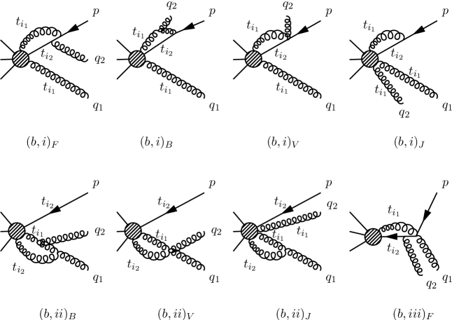
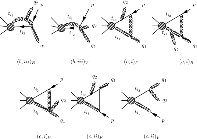
Figure 11: 1PI diagrams contributing to the mixing $J^{B2}_{{\cal A}\partial\chi}\to J^{C2}_{{\cal AA}\chi}$ of a $B$- into a $C$-type current in the collinear sector with fermion number $F_{i}=1$.

Several of the displayed diagrams are zero due to our choice of external momenta and polarization vectors:

• In diagram $(b,i)_{J}$ at least one of the external gluons is attached to a Wilson line, and it therefore vanishes.

• In diagram $(b,i)_{V}$, since the external gluon line with momentum $q_{1}$ has $\perp$ polarization, the internal gluon line picks up a factor $n_{+}$ from the Feynman rule for the gluon building block. When multiplying with the vertex (A.29), one obtains zero.

• Similarly, in diagram $(b,ii)_{J}$ both internal gluons come with factors of $n_{+}$. The three-gluon vertex (A.43) contracted as $n_{+}^{\rho}n_{+}^{\lambda}Q_{\rho\lambda\sigma}\epsilon_{1\perp}^{*\sigma}=0$ vanishes.

• In diagram $(b,ii)_{V}$ the internal gluon attached to the fermionic building block involves a factor $n_{+}$, and the one to the gluonic building block either $n_{+}$ or $\perp$, such that there are two possible contractions of the four-gluon vertex (A.53), $n_{+}^{\rho}n_{+}^{\lambda}Q_{\rho\lambda\sigma\kappa}\epsilon_{1\perp}^{*\sigma}\epsilon_{2\perp}^{*\kappa}=0$, $n_{+}^{\rho}g_{\perp}^{\mu\lambda}Q_{\rho\lambda\sigma\kappa}\epsilon_{1\perp}^{*\sigma}\epsilon_{2\perp}^{*\kappa}=0$ that both vanish.

• Diagram $(b,iii)_{V}$ involves a vertex with two collinear quarks and three collinear gluons. From the collinear SCET Lagrangian (A.1) one sees that at most two gluon fields can be transverse, hence in the above vertex at least one gluon comes from a Wilson line and therefore picks up a factor $n_{+}$. This has to be the internal line, since the two external line have $\perp$ polarization. Then the $n_{+}$ multiplied with the Feynman rule for the gluon building block vanishes.

The left-over diagrams are $(b,i)_{F/B}$, $(b,ii)_{B}$, $(b,iii)_{F/B}$, $(c,i/ii)_{F/V}$, $(c,i)_{B}$. In the limit $\epsilon\to 0$ they yield a single $1/\epsilon$ pole and are non-diagonal in momentum fractions and therefore contribute to the anomalous dimension. Some of them feature a simple pole singularity in collinear momentum fractions for particular configurations. We checked that these poles either cancel when adding up all diagrams, or lie outside of the support of Heaviside functions multiplying them. For example, $(c,i)_{F}$ has a single pole for $\bar{x}\to y_{2}$, that cancels with the corresponding pole of a diagram related to $(b,iii)_{B}$ by interchanging the external gluon lines. Further, $(c,ii)_{F}$ has single poles for $\bar{x}\to y_{2}$ and $x\to y_{3}$. The singularity $\propto 1/(y_{3}-x)$ cancels with $(b,iii)_{F}$, and the singularity $\propto 1/(\bar{x}-y_{2})$ with $(c,ii)_{V}$. Diagram $(c,ii)_{V}$ has a further singularity $\propto 1/(\bar{x}-y_{1})$ that cancels with the contribution analogous to $(c,ii)_{F}$ with interchanged external gluon lines. Note that the diagram $(c,ii)_{V}$ remains unchanged when interchanging external gluons, and therefore one should not add a diagram with permuted external lines in this case.

Figure 12: 1PR diagrams contributing to the mixing $J^{B2}_{{\cal A}\partial\chi}\to J^{C2}_{{\cal AA}\chi}$ of a $B$- into a $C$-type current in the collinear sector with fermion number $F_{i}=1$.

In addition, as in the previous section, 1PR diagrams for which the 1PR propagator is cancelled have to be included. The corresponding diagrams are shown in Fig. 12. Diagrams where external gluons are radiated off the external fermion line vanish for external momenta without $\perp$ component and pure $\perp$ polarization, due to the structure of the SCET vertex (A.28). The only non-zero contributions involving a 1PR fermion propagator are the last two.

All diagrams except the last one involve a three-gluon vertex. For these diagrams it is possible to first compute the corresponding diagram without the gluon splitting, and a single external gluon (using a polarization vector $\epsilon^{*\rho}$ and adjoint colour index $a$), which we denote by ${\cal M}_{\rho a}\epsilon^{*\rho}$. We keep all possible polarizations for $\epsilon^{*\rho}$, including also the longitudinal component (i.e. $\epsilon^{*}\cdot q\not=0$). The diagram with gluon splitting is then obtained by the replacement

$${\cal M}_{\rho a}\epsilon^{*\rho}\to{\cal M}_{\rho a}\frac{-ig_{s}}{q^{2}}f^{dea}\left((q_{2}-q_{1})^{\rho}\epsilon_{1}^{*}\cdot\epsilon_{2}^{*}-2\epsilon_{2}^{*\rho}\epsilon_{1}^{*}\cdot q_{2}+2\epsilon_{1}^{*\rho}\epsilon_{2}^{*}\cdot q_{1}\right)\,,$$ (4.17)

where $d(e)$ are the adjoint gluon colour indices for the two external gluons with momenta $q_{1}(q_{2})$ and polarization vectors $\epsilon_{1}^{*}(\epsilon_{2}^{*})$, and we used $\epsilon_{i}^{*}\cdot q_{i}=0$. Furthermore, $q\equiv q_{1}+q_{2}$ denotes the momentum of the 1PR propagator, and $p$ the momentum of the external outgoing antiquark.

The contribution of the 1PR diagrams to $B$-to-$C$ mixing corresponds to the divergent part which is not already accounted for by the time-ordered product of the 1PI subdiagram in on-shell kinematics with the three-gluon interaction. Consistency requires that this contribution must be local, that is, the $1/q^{2}$ from the 1PR gluon propagator must be cancelled. To extract this contribution, we have to temporarily restore $\perp$ components for the external momenta $q_{i}$, such that $q^{2}$ is independent from the small regulating offshellnesses $q_{i}^{2}\to 0$, $p^{2}\to 0$. This allows us to independently take the on-shell limit $q_{i}^{2},p^{2}\to 0$ at finite $q^{2}$ and then $q^{2}\to 0$. In this limit the relevant contribution from the 1PR diagrams becomes independent of the transverse momenta by power counting due to the homogeneous $\lambda$ scaling of all expressions. It is therefore possible and convenient to perform the calculation for the special configuration $q_{1\perp}=-q_{2\perp}$ such that $q=q_{1}+q_{2}$ has no $\perp$ component. The divergent contribution from the time-ordered product of the 1PI subdiagram in on-shell kinematics with the three-gluon interaction vanishes in this case. The reason is that the 1PI subdiagram in on-shell kinematics must be a $B2$ operator, i.e. is proportional to a linear combination of $q_{\perp}$ or $p_{\perp}$. Therefore, it vanishes for the kinematic configuration considered here, analogously to Eq. (4.16). This reduces our task to evaluating the 1PR diagrams in Fig. 12. The matrix element ${\cal M}_{\rho a}={\cal M}_{\rho a}(q,p)$ can be decomposed as

$${\cal M}_{\rho a}={\cal M}^{-}_{a}{n_{-}}_{\rho}+{\cal M}^{+}_{a}{n_{+}}_{\rho}+{\cal M}^{\perp}_{\rho a}\,.$$ (4.18)

With $q_{\rho}=\frac{1}{2}n_{+}\,q{n_{-}}_{\rho}+\frac{1}{2}n_{-}\,q{n_{+}}_{\rho}$ for $q_{\perp}=0$, we can always re-express the matrix element in the form

$${\cal M}_{\rho a}={\cal M}^{L}_{a}q_{\rho}+\tilde{\cal M}^{+}_{a}{n_{+}}_{\rho}+{\cal M}^{\perp}_{\rho a}\,,$$ (4.19)

where

$$\tilde{\cal M}^{+}_{a}={\cal M}^{+}_{a}-{\cal M}^{-}_{a}\frac{q^{2}}{(n_{+}q)^{2}}\;.$$ (4.20)

Then, using that $\epsilon_{i}=\epsilon_{i\perp}$ are assumed to be polarized in the $\perp$ direction, gives for the gluon splitting

$${\cal M}_{\rho a}\epsilon^{*\rho} \to \frac{-ig_{s}}{q^{2}}f^{dea}\,\Bigg{(}\!\left({\cal M}^{L}_{a}(q_{2}^{2}-q_{1}^{2})+\tilde{\cal M}^{+}_{a}n_{+}(q_{2}-q_{1})+{\cal M}^{\perp}_{a}\cdot(q_{2}-q_{1})_{\perp}\right)\epsilon_{1}^{*}\cdot\epsilon_{2}^{*}$$ (4.21)

$${}-2\epsilon_{2}^{*}\cdot{\cal M}^{\perp}_{a}\epsilon_{1}^{*}\cdot q_{2\perp}+2\epsilon_{1}^{*}\cdot{\cal M}^{\perp}_{a}\epsilon_{2}^{*}\cdot q_{1\perp}\Bigg{)}\,.$$

For ${\cal M}^{+}_{a}$, we find that the divergent part of the loop amplitude can be expanded for small $q^{2}$ and $p^{2}$ in the form

$${\cal M}^{+}_{a}={\cal M}^{+(p)}_{a}p^{2}+{\cal M}^{+(q)}_{a}q^{2}\,.$$ (4.22)

At this point we can take the on-shell limit $q_{i}^{2},p^{2}\to 0$ with $q^{2}$ finite, such that the first term in the bracket on the right-hand side of Eq. (4.21) vanishes, and ${\cal M}^{+(p)}_{a}$ in the previous equation can be dropped. After that, we can safely perform the limit $q_{i\perp}\to 0$, such that we finally arrive at the following rule,

$${\cal M}_{\rho a}\epsilon^{*\rho} \to -ig_{s}f^{dea}\left({\cal M}^{+(q)}_{a}-\frac{{\cal M}^{-}_{a}}{(n_{+}q)^{2}}\right)n_{+}(q_{2}-q_{1})\epsilon_{1}^{*}\cdot\epsilon_{2}^{*}\,.$$ (4.23)

The $1/q^{2}$ factor is manifestly cancelled in this expression, which therefore contributes to the mixing into a $C$-type operator.

In summary, we need to compute the matrix elements ${\cal M}^{\pm}_{a}$ for quark-gluon final states, for external momenta with vanishing $\perp$ components, and gluon polarization in the $\pm$ directions. This is different from the quark/gluon matrix elements computed in Sec. 4.3, and therefore we recomputed these diagrams for the required configuration of momenta and polarization vectors.

We find that the diagrams $(d,i)$ and $(d,ii)$ are proportional to $p^{2}/q^{2}$ (i.e. only ${\cal M}^{+(p)}_{a}$ is non-zero), and therefore vanish for $p^{2}\to 0$. For $(d,iii)$ only ${\cal M}^{+(q)}_{a}$ is non-zero, i.e. it gives a contribution to the anomalous dimension. Diagram $(d,iv)$ gives ${\cal M}_{\rho a}\propto(p+q)^{2}$ which can be brought in the form (4.22) using $(p+q)^{2}=n_{+}(p+q)n_{-}(p+q)=\frac{p^{2}}{y_{3}}+\frac{q^{2}}{y_{1}+y_{2}}$. For diagrams $(d,v)$ and $(d,vi)$ both ${\cal M}^{-}_{a}$ and ${\cal M}^{+(q)}_{a}$ yield non-zero contributions. A singularity $\propto\gamma_{\perp}^{\nu}\gamma_{\perp}^{\mu}/(y_{3}-x)$ cancels in the sum of $(d,vi)$ and $(d,iv)$.

For diagram $(d,vii)$ only ${\cal M}^{-}_{a}$ is non-zero. Still, the loop gives an additional factor $(p+q)^{2}$, that however cancels with the 1PR fermion propagator. Therefore this diagram also contributes. Finally, the diagram $(d,viii)$ is special because it does not contain a three-gluon vertex. A direct computation shows that the 1PR fermion propagator cancels with a factor $(p+q)^{2}$ obtained from the loop integral, similar as for $(d,vii)$.

As discussed before, counterterm diagrams involving $A$- and $B$-type operators necessarily involve some powers of external $\perp$ momenta, and therefore vanish. The only non-zero counterterm diagram is therefore the one involving $J^{C2}_{{\cal A}^{\mu}{\cal A}^{\nu}\chi}$,

$$\langle g_{d}(q_{1})g_{e}(q_{2})\bar{q}(p)|J^{C2}_{{\cal A}^{\mu b}{\cal A}^{\nu c}\chi}|0\rangle_{\rm tree} = g_{s}^{2}e^{i(t_{i_{1}}n_{+}q_{1}+t_{i_{2}}n_{+}q_{2}+t_{i_{3}}n_{+}p)}\epsilon_{1}^{*\mu}\epsilon_{2}^{*\nu}\delta_{bd}\delta_{ce}v_{c}$$ (4.24)

$${}+(q_{1},d,\epsilon_{1}^{*}\leftrightarrow q_{2},e,\epsilon_{2}^{*})\,,$$

where we made explicit the (adjoint) colour indices for external gluons and gluon building blocks. After Fourier transformation with respect to the $t_{i_{j}}$ (with $y_{3}=1-y_{1}-y_{2}$),

$$\langle g_{d}(q_{1})g_{e}(q_{2})\bar{q}(p)|J^{C2}_{{\cal A}^{\mu b}{\cal A}^{\nu c}\chi}(y_{1},y_{2})|0\rangle_{\rm tree}$$ (4.25)

$$= P_{i}^{3}g_{s}^{2}\delta(P_{i}y_{1}-n_{+}q_{1})\delta(P_{i}y_{2}-n_{+}q_{2})\delta(P_{i}y_{3}-n_{+}p)\epsilon_{1}^{*\mu}\epsilon_{2}^{*\nu}\delta_{bd}\delta_{ce}v_{c}$$

$${}+(q_{1},d,\epsilon_{1}^{*}\leftrightarrow q_{2},e,\epsilon_{2}^{*})$$

$$= P_{i}g_{s}^{2}\delta(y_{1}-\hat{y}_{1})\delta(y_{2}-\hat{y}_{2})\delta(P_{i}-n_{+}(q_{1}+q_{2}+p))\epsilon_{1}^{*\mu}\epsilon_{2}^{*\nu}\delta_{bd}\delta_{ce}v_{c}$$

$${}+(q_{1},d,\epsilon_{1}^{*}\leftrightarrow q_{2},e,\epsilon_{2}^{*})\,.$$

Here we defined the momentum fractions $\hat{y}_{1(2)}\equiv n_{+}q_{1(2)}/n_{+}(p+q_{1}+q_{2})$ via the external momenta.

On the other hand, the divergent part of the one-loop matrix element of $J^{B2}_{{\cal A}^{\mu a}\partial^{\nu}\xi}$ can be written in the form

$$\langle g_{d}(q_{1})g_{e}(q_{2})\bar{q}(p)|J^{B2}_{{\cal A}^{\mu a}\partial^{\nu}\chi}|0\rangle_{\rm 1-loop}^{\rm div}$$ (4.26)

$$= \frac{g_{s}^{4}}{16\pi^{2}\epsilon}\int_{0}^{1}dx^{\prime}e^{i(t_{i_{1}}x^{\prime}+t_{i_{2}}\bar{x}^{\prime})n_{+}(q_{1}+q_{2}+p)}I_{ade}^{\mu\nu\sigma\lambda}(x^{\prime},\hat{y}_{1},\hat{y}_{2})\epsilon_{1}^{*\sigma}\epsilon_{2}^{*\lambda}v_{c}\,,$$

which defines the function $I_{ade}^{\mu\nu\sigma\lambda}(x^{\prime},\hat{y}_{1},\hat{y}_{2})$. After Fourier transformation,

$$\langle g_{d}(q_{1})g_{e}(q_{2})\bar{q}(p)|J^{B2}_{{\cal A}^{\mu a}\partial^{\nu}\chi}(x)|0\rangle_{\rm 1-loop}^{\rm div}$$ (4.27)

$$= P_{i}^{2}\frac{g_{s}^{4}}{16\pi^{2}\epsilon}\int_{0}^{1}dx^{\prime}\delta(P_{i}x-x^{\prime}n_{+}(q_{1}+q_{2}+p))\delta(P_{i}\bar{x}-\bar{x}^{\prime}n_{+}(q_{1}+q_{2}+p))$$

$$\times\,I_{ade}^{\mu\nu\sigma\lambda}(x^{\prime},\hat{y}_{1},\hat{y}_{2})\epsilon_{1}^{*\sigma}\epsilon_{2}^{*\lambda}v_{c}$$

$$= P_{i}\frac{g_{s}^{4}}{16\pi^{2}\epsilon}\delta(P_{i}-n_{+}(q_{1}+q_{2}+p))I_{ade}^{\mu\nu\sigma\lambda}(x,\hat{y}_{1},\hat{y}_{2})\epsilon_{1}^{*\sigma}\epsilon_{2}^{*\lambda}v_{c}$$

$$= \frac{g_{s}^{2}}{16\pi^{2}\epsilon}\frac{1}{2}\int dy_{1}dy_{2}\,I_{abc}^{\mu\nu\sigma\lambda}(x,y_{1},y_{2})\,\langle g_{d}(q_{1})g_{e}(q_{2})\bar{q}(p)|J^{C2}_{{\cal A}^{\sigma b}{\cal A}^{\lambda c}\chi}(y_{1},y_{2})|0\rangle_{\rm tree}\,,\qquad$$

where in the last step we used that $I_{ade}^{\mu\nu\sigma\lambda}(x,y_{1},y_{2})=I_{aed}^{\mu\nu\lambda\sigma}(x,y_{2},y_{1})$ due to symmetry under exchange of the two external gluon lines, leading to the additional factor $1/2$. From the last relation we can read off the anomalous dimension,

$$\gamma^{i}_{{\cal A}^{\mu a}\partial^{\nu}\xi,{\cal A}^{\sigma d}{\cal A}^{\lambda e}\xi}(x,y_{1},y_{2})=-\frac{\alpha_{s}}{8\pi}\,I_{ade}^{\mu\nu\sigma\lambda}(x,y_{1},y_{2})\,.$$ (4.28)

From the explicit one-loop results one can read off $I_{ade}^{\mu\nu\sigma\lambda}(x,y_{1},y_{2})$. The results are provided in App. C.2.1.

4.4.2 Mixing $J^{B2}_{{\cal A}\partial\chi}(x)\to J^{C2}_{\chi\bar{\chi}\chi}(y_{1},y_{2})$

For this case we consider the matrix element of the current with three fermions, two outgoing antiquarks and one outgoing quark, all with external momenta that have vanishing $\perp$ components. For simplicity we assume that the third fermionic building block has a different flavour from the first two, and comment on the generalization below.

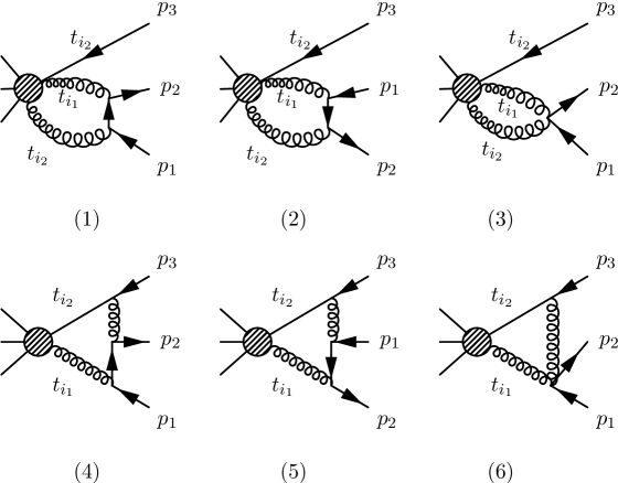
Figure 13: 1PI diagrams contributing to the mixing $J^{B2}_{{\cal A}\partial\chi}\to J^{C2}_{\chi\bar{\chi}\chi}$ of a $B$- into a $C$-type current in the collinear sector with fermion number $F_{i}=1$.

The relevant 1PI diagrams are shown in Fig. 13. Diagram (3) vanishes, because the gluon line attached to the fermionic building block (label $t_{i_{2}}$) picks up a factor $n_{+}$ from the Wilson line, and this gives zero when multiplied with the two-fermion vertex. Diagram (1) would become singular for $x\to\bar{y}_{3}\equiv y_{1}+y_{2}$, but one can check that the Heaviside functions obtained from the collinear loop vanish in the domain of the pole for $0<y_{i}<1$. Furthermore, a potential singularity for $x\to y_{1}$ cancels in the sum of (4) and (6), and for $x\to y_{2}$ in the sum of (5) and (6).

The relevant 1PR diagrams are similar to the 1PR diagrams shown in Fig. 12 for the $qgg$ final state. They can be obtained by replacing the three-gluon vertex attached to 1PR gluon propagator by a fermion-fermion-gluon vertex for diagram $(d,i)$ to $(d,vii)$. Diagram $(d,viii)$ does not exist for the $q\bar{q}q$ final state. As before, we can infer the contribution from the matrix element ${\cal M}_{\rho a}\epsilon^{*\rho}$ of quark-gluon final states obtained by cutting the 1PR gluon propagator. For vanishing external $\perp$ momenta, taking the $g\to\bar{q}q$ splitting into account amounts to (assuming the same-flavour antiquark and quark attached to the 1PR propagator have momenta $p_{1}$ and $p_{2}$, respectively)

$${\cal M}_{\rho a}\epsilon^{*\rho}\to{\cal M}_{\rho a}\frac{-i}{q^{2}}\bar{u}_{c}(p_{2})ig_{s}t^{a}\left(n_{-}^{\rho}+\frac{\not{p}_{2\perp}\gamma_{\perp}^{\rho}}{n_{+}p_{2}}+\frac{\gamma_{\perp}^{\rho}\not{p}_{1\perp}}{n_{+}p_{1}}-n_{+}^{\rho}\frac{\not{p}_{2\perp}\not{p}_{1\perp}}{n_{+}p_{1}n_{+}p_{2}}\right)\frac{\not{n}_{+}}{2}v_{c}(p_{1})\,,$$ (4.29)

where now $q=p_{1}+p_{2}$ is the momentum through the 1PR propagator. In order to be able to take the limit $p_{1}^{2}\to 0$ and $p_{2}^{2}\to 0$ with $q^{2}=(p_{1}+p_{2})^{2}$ finite, we introduce again for a moment a non-zero $\perp$ momentum such that $p_{1\perp}=-p_{2\perp}$. Then, as before, the matrix element ${\cal M}_{\rho a}={\cal M}_{\rho a}(q,p_{3})$ is independent of the $\perp$ momenta. Using the decomposition (4.19) we get

$${\cal M}_{\rho a}\epsilon^{*\rho} \to \frac{-i}{q^{2}}\bar{u}_{c}(p_{2})ig_{s}t^{a}$$ (4.30)

$$\times\,\left(2\tilde{\cal M}^{+}_{a}+\frac{\not{p}_{2\perp}\not{\cal M}_{a}^{\perp}}{n_{+}p_{2}}+\frac{\not{\cal M}_{a}^{\perp}\not{p}_{1\perp}}{n_{+}p_{1}}+{\cal M}_{a}^{L}\left(\frac{p_{1}^{2}}{n_{+}p_{1}}+\frac{p_{2}^{2}}{n_{+}p_{2}}\right)\right)\frac{\not{n}_{+}}{2}v_{c}(p_{1})\,.$$

At this point we can take the limit $p_{i}^{2}\to 0$, and afterwards let the $\perp$ momenta go to zero again, obtaining

$${\cal M}_{\rho a}\epsilon^{*\rho} \to \frac{g_{s}}{q^{2}}\left({\cal M}^{+(q^{2})}_{a}q^{2}-{\cal M}^{-}_{a}\frac{q^{2}}{(n_{+}q)^{2}}\right)\bar{u}_{c}(p_{2})t^{a}\not{n}_{+}v_{c}(p_{1})\,,$$ (4.31)

where we used Eqs. (4.20) and (4.22) with $p\mapsto p_{3}$. As for the $qgg$ case, the 1PR momentum $q^{2}$ cancels and we obtain a finite result. The result for all 1PR diagrams $(d,i)$ to $(d,vii)$ can therefore be obtained from the corresponding $qgg$ final state by replacing

$$-if^{dea}(y_{2}-y_{1})\epsilon_{1}^{*}\cdot\epsilon_{2}^{*}\mapsto\frac{1}{P_{i}}\bar{u}_{c}(p_{2})t^{a}\not{n}_{+}v_{c}(p_{1})\,.$$ (4.32)

The tree-level contribution from the $C$-type operator is (displaying colour and Dirac indices and accounting for signs from anticommutations)

$$\langle\bar{q}(p_{1})q(p_{2})\bar{q}(p_{3})|J^{C2}_{\xi^{\beta}_{j}\bar{\xi}^{\gamma}_{k}\xi^{\delta}_{l}}|0\rangle_{\rm tree}=(-1)e^{i(t_{i_{1}}n_{+}p_{1}+t_{i_{2}}n_{+}p_{2}+t_{i_{3}}n_{+}p_{3})}v_{cj}^{\beta}(p_{1})\bar{u}_{ck}^{\gamma}(p_{2})v_{cl}^{\delta}(p_{3})\,.$$ (4.33)

The loop amplitude for the sum of the 1PI and 1PR diagrams can be written as (we extract a factor $1/P_{i}$ of total collinear momentum for later convenience, for dimensional reasons, and $\hat{y}_{i}\equiv n_{+}p_{i}/n_{+}(p_{1}+p_{2}+p_{3})$)

$$\langle\bar{q}(p_{1})q(p_{2})\bar{q}(p_{3})|J^{B2}_{{\cal A}^{\mu a}\partial^{\nu}\xi^{\alpha}_{i}}|0\rangle_{\rm 1-loop}^{\rm div}$$ (4.34)

$$= \frac{g_{s}^{4}}{16\pi^{2}\epsilon}\frac{1}{P_{i}}\int_{0}^{1}dx^{\prime}\,e^{i(t_{i_{1}}x^{\prime}+t_{i_{2}}\bar{x}^{\prime})n_{+}(p_{1}+p_{2}+p_{3})}I_{aijkl}^{\mu\nu\alpha\beta\gamma\delta}(x^{\prime},\hat{y}_{1},\hat{y}_{2})v_{cj}^{\beta}(p_{1})\bar{u}_{ck}^{\gamma}(p_{2})v_{cl}^{\delta}(p_{3})\,,\qquad$$

which defines the kernel $I_{aijkl}^{\mu\nu\alpha\beta\gamma\delta}(x,\hat{y}_{1},\hat{y}_{2})$. After Fourier transformation,

$$\langle\bar{q}(p_{1})q(p_{2})\bar{q}(p_{3})|J^{B2}_{{\cal A}^{\mu a}\partial^{\nu}\xi^{\alpha}_{i}}(x)|0\rangle_{\rm 1-loop}^{\rm div}$$

$$= {}-\frac{g_{s}^{4}}{16\pi^{2}\epsilon}\frac{1}{P_{i}}\int dy_{1}dy_{2}\,I_{aijkl}^{\mu\nu\alpha\beta\gamma\delta}(x,y_{1},y_{2})\,\langle\bar{q}(p_{1})q(p_{2})\bar{q}(p_{3})|J^{C2}_{\xi^{\beta}_{j}\bar{\xi}^{\gamma}_{k}\xi^{\delta}_{l}}(y_{1},y_{2})|0\rangle_{\rm tree}\,.$$

From this relation, the anomalous dimension can be read off,

$$\gamma^{i}_{{\cal A}^{\mu a}\partial^{\nu}\chi^{\alpha}_{i},\chi^{\beta}_{j}\bar{\chi}^{\gamma}_{k}\chi^{\delta}_{l}}(x,y_{1},y_{2})=\frac{\alpha_{s}}{8\pi}g_{s}^{2}\frac{1}{P_{i}}I_{aijkl}^{\mu\nu\alpha\beta\gamma\delta}(x,y_{1},y_{2})\,.$$ (4.36)

The factor $g_{s}^{2}$ is due to our convention for the normalization of the collinear building blocks, and the factor $1/P_{i}$ of the total collinear momentum arises for dimensional reasons. The results for $I_{aijkl}^{\mu\nu\alpha\beta\gamma\delta}(x,y_{1},y_{2})$ are collected in App. C.2.2.

If all fermion building blocks are of the the same flavour, the expression on the right-hand side needs to be anti-symmetrized with respect to interchanging the first and the last building block, i.e.

$$I_{aijkl}^{\mu\nu\alpha\beta\gamma\delta}(x,y_{1},y_{2})\to\frac{1}{2}\left[I_{aijkl}^{\mu\nu\alpha\beta\gamma\delta}(x,y_{1},y_{2})-I_{ailkj}^{\mu\nu\alpha\delta\gamma\beta}(x,y_{3},y_{2})\right]\,,$$ (4.37)

where, as before, $y_{3}=1-y_{1}-y_{2}$.

4.5 Mixing of $C$-type currents into $C$-type currents

As discussed in Ref. [14], at the one-loop order, this mixing arises from diagrams for which only two out of the three building blocks of the $C$-type current are attached to lines belonging to the loop. Therefore, the anomalous dimension can be obtained from the one of the corresponding $B$-type currents at ${\cal O}(\lambda)$. We denote the independent momentum fractions of the first and second collinear building block by $x_{1}\equiv x_{i_{1}}$ and $x_{2}\equiv x_{i_{2}}$, and set $x_{3}=1-x_{1}-x_{2}$ for the third one. For example, for $J^{C2}_{{\cal AA}\chi}$ $x_{3}$ denotes the fraction of collinear momentum carried by the fermion. For the anomalous dimension that corresponds to $J^{C2}_{{\cal AA}\chi}(x_{1},x_{2})\to J^{C2}_{{\cal AA}\chi}(y_{1},y_{2})$ the momentum fractions $y_{1,2,3}$ of the second operator are defined analogously, and we find

$$\gamma^{i}_{{\cal A}^{\mu}{\cal A}^{\nu}\chi_{\alpha},{\cal A}^{\rho}{\cal A}^{\sigma}\chi_{\beta}}(x_{1},x_{2},y_{1},y_{2}) = \Bigg{[}\frac{1}{1-y_{2}}\delta(x_{2}-y_{2})g_{\perp}^{\nu\sigma}\gamma^{i}_{{\cal A}^{\mu}\chi_{\alpha},{\cal A}^{\rho}\chi_{\beta}}\left(\frac{x_{1}}{1-x_{2}},\frac{y_{1}}{1-y_{2}}\right)$$ (4.38)

$$+\,\frac{1}{1-y_{1}}\delta(x_{1}-y_{1})g_{\perp}^{\mu\rho}\gamma^{i}_{{\cal A}^{\nu}\chi_{\alpha},{\cal A}^{\sigma}\chi_{\beta}}\left(\frac{x_{2}}{1-x_{1}},\frac{y_{2}}{1-y_{1}}\right)$$

$$+\,\frac{1}{1-y_{3}}\delta(x_{3}-y_{3})\delta_{\alpha\beta}\gamma^{i}_{{\cal A}^{\mu}{\cal A}^{\nu},{\cal A}^{\rho}{\cal A}^{\sigma}}\left(\frac{x_{1}}{1-x_{3}},\frac{y_{1}}{1-y_{3}}\right)\Bigg{]}_{\rm sym}\,.$$

Here the square bracket refers to symmetrization with respect to $(y_{1},\rho,b_{1})\leftrightarrow(y_{2},\sigma,b_{2})$ where $b_{1}$ ($b_{2}$) denotes the adjoint colour index carried by the gluon building block ${\cal A}^{\rho}$ (${\cal A}^{\sigma}$). These indices are left implicit in the equation above, including a Kronecker symbol for the colour indices of the two gluon building blocks not contained in $\gamma^{i}_{{\cal A}^{\mu}\chi_{\alpha},{\cal A}^{\rho}\chi_{\beta}}$ or $\gamma^{i}_{{\cal A}^{\nu}\chi_{\alpha},{\cal A}^{\sigma}\chi_{\beta}}$ in the first and second line, respectively. A similar statement refers to the quark fields in the third line and the equations below in this section. Symmetrization refers here to the average over the expression given in the square bracket, and the corresponding expression obtained when replacing $(y_{1},\rho,b_{1})\to(y_{2},\sigma,b_{2})$, i.e. includes a normalization factor $1/2$. The anomalous dimension $\gamma^{i}_{{\cal A}^{\mu}{\cal A}^{\nu},{\cal A}^{\rho}{\cal A}^{\sigma}}$ will be provided in a future work dedicated to the case of fermion number $F_{i}=0$.

The mixing $J^{C2}_{{\cal AA}\chi}(x_{1},x_{2})\to J^{C2}_{\chi\bar{\chi}\chi}(y_{1},y_{2})$ vanishes if we assume that all fermions in the latter operator carry a different flavour quantum number. If the fermions $\chi\bar{\chi}$ are of the same flavour, and the fermion in the last building block has a different flavour, we find

$$\gamma^{i}_{{\cal A}^{\mu}{\cal A}^{\nu}\chi_{\alpha},\chi_{\beta}\bar{\chi}_{\gamma}\chi_{\delta}}(x_{1},x_{2},y_{1},y_{2})=-\frac{1}{1-y_{3}}\delta(x_{3}-y_{3})\delta_{\alpha\delta}\,\gamma^{i}_{{\cal A}^{\mu}{\cal A}^{\nu},\bar{\chi}_{\gamma}\chi_{\beta}}\left(\frac{x_{1}}{1-x_{3}},\frac{y_{2}}{1-y_{3}}\right)\,.$$ (4.39)

Note the minus sign due to the interchange of fermion indices. For $\gamma^{i}_{{\cal A}^{\mu}{\cal A}^{\nu},\bar{\chi}_{\gamma}\chi_{\beta}}$ we also refer to future work on the $F_{i}=0$ case. If all fermions are of the same flavour, the anomalous dimension can be obtained by antisymmetrizing Eq. (4.39) with respect to $(y_{1},\beta,c_{1})\leftrightarrow(y_{3},\delta,c_{3})$, where $c_{k}$ denote the fundamental colour indices of the first and third fermion building block, respectively. As before, antisymmetrization is understood to include a normalization factor $1/2$.

For the contribution corresponding to $J^{C2}_{\chi\bar{\chi}\chi}(x_{1},x_{2})\to J^{C2}_{\chi\bar{\chi}\chi}(y_{1},y_{2})$, we find for the case where the first and last building blocks carry distinct flavour,

$$\gamma^{i}_{\chi_{\alpha}\bar{\chi}_{\beta}\chi_{\gamma},\chi_{\alpha^{\prime}}\bar{\chi}_{\beta^{\prime}}\chi_{\gamma^{\prime}}}(x_{1},x_{2},y_{1},y_{2}) = \frac{1}{1-y_{2}}\delta(x_{2}-y_{2})\delta_{\beta\beta^{\prime}}\gamma^{i}_{\chi_{\alpha}\chi_{\gamma},\chi_{\alpha^{\prime}}\chi_{\gamma^{\prime}}}\left(\frac{x_{1}}{1-x_{2}},\frac{y_{1}}{1-y_{2}}\right)$$ (4.40)

$$+\,\frac{1}{1-y_{1}}\delta(x_{1}-y_{1})\delta_{\alpha\alpha^{\prime}}\gamma^{i}_{\bar{\chi}_{\beta}\chi_{\gamma},\bar{\chi}_{\beta^{\prime}}\chi_{\gamma^{\prime}}}\left(\frac{x_{2}}{1-x_{1}},\frac{y_{2}}{1-y_{1}}\right)$$

$$+\,\frac{1}{1-y_{3}}\delta(x_{3}-y_{3})\delta_{\gamma\gamma^{\prime}}\gamma^{i}_{\bar{\chi}_{\beta}\chi_{\alpha},\bar{\chi}_{\beta^{\prime}}\chi_{\alpha^{\prime}}}\left(\frac{x_{2}}{1-x_{3}},\frac{y_{2}}{1-y_{3}}\right)\,.$$

Note that the last line requires two fermion permutations leading to the positive sign, and that even for the case of different flavour quantum numbers three distinct loop contributions exist that lead to the three terms on the right-hand side. For $\gamma^{i}_{\chi_{\alpha}\chi_{\gamma},\chi_{\alpha^{\prime}}\chi_{\gamma^{\prime}}}$ we refer to Ref. [14], and for $\gamma^{i}_{\bar{\chi}_{\beta}\chi_{\alpha},\bar{\chi}_{\beta^{\prime}}\chi_{\alpha^{\prime}}}$ to future work on the $F_{i}=0$ case. If the flavour of the fermions in the first and last building block are identical, one needs to antisymmetrize the right-hand side with respect to $(y_{1},\beta,c_{1})\leftrightarrow(y_{3},\delta,c_{3})$ as before.

For $J^{C2}_{\chi\bar{\chi}\chi}(x_{1},x_{2})\to J^{C2}_{{\cal AA}\chi}(y_{1},y_{2})$ we first provide the result obtained if all fermions have identical flavour,

$$\gamma^{i}_{\chi_{\alpha}\bar{\chi}_{\beta}\chi_{\gamma},{\cal A}^{\mu}{\cal A}^{\nu}\chi_{\delta}}(x_{1},x_{2},y_{1},y_{2}) = \frac{1}{1-y_{3}}\delta(x_{1}-y_{3})\delta_{\alpha\delta}\gamma^{i}_{\bar{\chi}_{\beta}\chi_{\gamma},{\cal A}^{\mu}{\cal A}^{\nu}}\left(\frac{x_{2}}{1-x_{1}},\frac{y_{1}}{1-y_{3}}\right)$$ (4.41)

$$-\,\frac{1}{1-y_{3}}\delta(x_{3}-y_{3})\delta_{\gamma\delta}\gamma^{i}_{\bar{\chi}_{\beta}\chi_{\alpha},{\cal A}^{\mu}{\cal A}^{\nu}}\left(\frac{x_{2}}{1-x_{3}},\frac{y_{1}}{1-y_{3}}\right)\,.$$

If the first fermion $\chi_{\alpha}$ has a different flavour from the other two, only the first line contributes on the right-hand side. If, on the other hand, the third fermion $\chi_{\gamma}$ has a different flavour, only the second line contributes. In this case we do not need to explicitly symmetrize with respect to interchanging the gluonic building blocks, because this symmetrization is already taken care of in the anomalous dimension $\gamma^{i}_{\bar{\chi}_{\alpha}\chi_{\beta},{\cal A}^{\mu}{\cal A}^{\nu}}$.

Finally, we discuss the case $F_{i}=3$, where the only the mixing $J^{C2}_{\chi\chi\chi}(x_{1},x_{2})\to J^{C2}_{\chi\chi\chi}(y_{1},y_{2})$ is possible. For three fermions with mutually distinct flavour quantum numbers, the result has the expected form

$$\gamma^{i}_{\chi_{\alpha}\chi_{\beta}\chi_{\gamma},\chi_{\alpha^{\prime}}\chi_{\beta^{\prime}}\chi_{\gamma^{\prime}}}(x_{1},x_{2},y_{1},y_{2}) = \frac{1}{1-y_{2}}\delta(x_{2}-y_{2})\delta_{\beta\beta^{\prime}}\gamma^{i}_{\chi_{\alpha}\chi_{\gamma},\chi_{\alpha^{\prime}}\chi_{\gamma^{\prime}}}\left(\frac{x_{1}}{1-x_{2}},\frac{y_{1}}{1-y_{2}}\right)$$ (4.42)

$$+\,\frac{1}{1-y_{1}}\delta(x_{1}-y_{1})\delta_{\alpha\alpha^{\prime}}\gamma^{i}_{\chi_{\beta}\chi_{\gamma},\chi_{\beta^{\prime}}\chi_{\gamma^{\prime}}}\left(\frac{x_{2}}{1-x_{1}},\frac{y_{2}}{1-y_{1}}\right)$$

$$+\,\frac{1}{1-y_{3}}\delta(x_{3}-y_{3})\delta_{\gamma\gamma^{\prime}}\gamma^{i}_{\chi_{\alpha}\chi_{\beta},\chi_{\alpha^{\prime}}\chi_{\beta^{\prime}}}\left(\frac{x_{1}}{1-x_{3}},\frac{y_{1}}{1-y_{3}}\right)\,.$$

If, for example, the first and last fermion have identical flavour the right-hand side needs to be antisymmetrized with respect to the interchange of the corresponding momentum fractions and Dirac as well as colour indices $(y_{1},\alpha^{\prime},c_{1})\leftrightarrow(y_{3},\gamma^{\prime},c_{3})$. If all three fermions have identical flavour, the right-hand side needs to be fully antisymmetrized with respect to all possible $3!$ permutations, including a normalization factor $1/6$ and a minus sign for odd permutations, due to fermion anticommutation.

5 Summary

In this work we extended the computation of the one-loop anomalous dimension matrix of subleading-power $N$-jet operators started in Ref. [14]. The operator basis can be characterized by the number and type of collinear building blocks for each of the $N$ collinear directions. In addition, homogeneous power counting in $\lambda$ of the anomalous dimension requires to take into account time-ordered products of $N$-jet currents with insertions of the power-suppressed terms ${\cal L}^{(n)}$ of the SCET Lagrangian. The general structure of the anomalous dimension matrix (2.17) encompasses universal contributions that are diagonal with respect to collinear momentum and the type of operators, as well as off-diagonal contributions. The latter can be divided into a contribution $\gamma^{i}$ that describes current-current mixing and arises from collinear loops along the $i$ direction, and $\gamma^{ij}$ that captures mixing of time-ordered products into currents. It originates from soft loops connecting directions $i$ and $j$, and represents a qualitatively new feature compared to Ref. [14]. In this work we provide complete results for $\gamma^{i}$ for currents with fermion number $|F_{i}|=1,3$ in direction $i$, and for $\gamma^{ij}$ for $|F_{i}|=|F_{j}|=1$. In addition, we find several general properties of $\gamma^{ij}$:

• Time-ordered products containing a single insertion of ${\cal L}^{(1)}$ or ${\cal L}^{(2)}$, or double insertions along a single collinear direction, do not mix into currents. This implies in particular that $\gamma^{ij}$ vanishes at order $\lambda$.

• Time-ordered products involving power-suppressed interactions of massless soft quarks, given by ${\cal L}^{(1)}_{\xi q}$, also do not mix into currents. As a consequence, fermion number is conserved separately for every collinear direction in the massless theory.

• For $|F_{i}|=|F_{j}|=1$, operators containing a product of two time-ordered products $J^{T1}J^{T1}$ in directions $i$ and $j$ can only mix into a product of two ${\cal O}(\lambda)$ currents $J^{X1}J^{Y1}$ with $X,Y=A,B$, but not into $J^{X2}J^{A0}$ with $X=A,B,C$. Thus we observe that the level of power suppression is also “conserved” along each collinear direction.

Altogether, non-zero contributions to $\gamma^{ij}$ can arise only from time-ordered products containing an insertion of ${\cal L}^{(1)}_{\xi}$ or ${\cal L}^{(1)}_{\rm YM}$ along direction $i$, and another one along direction $j$. For the case $F_{i}=F_{j}=1$ the structure of $\gamma^{ij}$ is therefore given by

$$\gamma^{ij}_{PQ}\quad=\quad\begin{array}[]{c||cccc|cc|}&J^{A1}_{\partial\chi}J^{A1}_{\partial\chi}&J^{B1}_{{\cal A}\chi}J^{A1}_{\partial\chi}&J^{A1}_{\partial\chi}J^{B1}_{{\cal A}\chi}&J^{B1}_{{\cal A}\chi}J^{B1}_{{\cal A}\chi}&J^{X2}J^{A0}&J^{A0}J^{X2}\\ \hline\cr\hline\cr J^{T1}_{\chi,\xi}\;J^{T1}_{\chi,\xi}&\eqref{eq:T1xiT1xi_A1A1}&\eqref{eq:T1xiT1xi_B1A1}&\eqref{eq:T1xiT1xi_B1A1}&\eqref{eq:T1xiT1xi_B1B1}&0&0\\ J^{T1}_{\chi,\rm YM}\;J^{T1}_{\chi,\xi}&0&\eqref{eq:T1YMT1xi_B1A1}&0&\eqref{eq:T1YMT1xi_B1B1}&0&0\\ J^{T1}_{\chi,\xi}\;J^{T1}_{\chi,\rm YM}&0&0&\eqref{eq:T1YMT1xi_B1A1}&\eqref{eq:T1YMT1xi_B1B1}&0&0\\ J^{T1}_{\chi,\rm YM}\;J^{T1}_{\chi,\rm YM}&0&0&0&\eqref{eq:T1YMT1YM_B1B1}&0&0\\ \hline\cr J^{T2}\;J^{A0}&0&0&0&0&0&0\\ J^{T1}\;J^{Y1}&0&0&0&0&0&0\\ J^{T1}_{\chi,\xi q}\;J^{T1}&0&0&0&0&0&0\\[5.69046pt] \end{array}\quad$$ (5.9)

where $X=A,B,C$ and $Y=A,B$. The non-zero entries refer to the equation numbers in which the result is given or to which it is related up to interchanging $i\leftrightarrow j$. For $F_{i}=-1$ or $F_{j}=-1$ the anomalous dimension is obtained by hermitian conjugation (see App. D for details). For $F_{i}=-F_{j}$ mixing into operators with $F_{i}=F_{j}=0$ via soft quark exchange vanishes due to the conservation of fermion number along each collinear direction as observed above.

Apart from the soft contributions to the anomalous dimension, we provide results for the collinear part $\gamma^{i}$. For this part we find that it is sufficient to consider current-current mixing. Mixing of time-ordered products into currents vanishes in the collinear sector, while mixing of time-ordered products into themselves is identical to the corresponding current-current mixing. Furthermore, collinear loops involve only a single collinear direction, denoted by $i$. The operator basis for $F_{i}=1$ contains two operators at ${\cal O}(\lambda)$ (one $A$- and one $B$-type), and five at ${\cal O}(\lambda^{2})$ (one $A$-, two $B$- and two $C$-type). The corresponding $2\times 2$ and $5\times 5$ matrices $\gamma^{i}_{PQ}$ are given in Eq. (4.1) and in Eq. (4.8), respectively. The latter contains non-zero mixings of the form $J^{B2}\to J^{B2},J^{C2}$ and $J^{C2}\to J^{C2}$. Operators with fermion number $F_{i}=3$ start at ${\cal O}(\lambda^{2})$, see Eq. (4.42).

To complete the one-loop renormalization programme of ${\cal O}(\lambda^{2})$ SCET $N$-jet operators, the calculation of the anomalous dimension in the $F=0$ sector is required. This includes the case of gluon jets at leading power and the mixing of two-gluon into quark-antiquark $B1$-type operators at the power-suppressed level. Work on this is in progress. It should then be feasible to consider next-to-leading logarithmic resummation of power corrections to jet processes of the SCET_I type.

Acknowledgements

We thank A. Broggio and S. Jaskiewicz for useful discussions. This work has been supported by the Bundesministerium für Bildung und Forschung (BMBF) grant nos. 05H15WOCAA and 05H18WOCA1.

Appendix A SCET Feynman rules

A.1 Preliminaries

In this appendix we give explicit expressions for the Feynman rules in the position-space formulation of SCET [23] up to ${\cal O}(\lambda^{2})$, derived from the multipole-expanded Lagrangian given in Ref. [24]. The field content consists of collinear quarks ($\xi$) with scaling $\xi\sim\lambda$, collinear gluons ($A_{c}$) with scaling $(n_{+}A_{c},A_{c\perp},n_{-}A_{c})\sim(1,\lambda,\lambda^{2})$, soft quarks ($q\sim\lambda^{3}$) and soft gluons ($A_{s}\sim\lambda^{2}$). The Lagrangian can be split into a purely bosonic part ${\cal L}_{\rm YM}$ and a part involving fermions (denoted by ${\cal L}$). Each part can be expanded in powers of $\lambda$ [24]

$${\cal L}=\bar{\xi}\left(in_{-}D+i\not{D}_{\perp}\frac{1}{in_{+}D}i\not{D}_{\perp}\right)\frac{\not{n}_{+}}{2}\xi+\bar{q}i\not{D}_{s}q+{\cal L}_{\xi}^{(1)}+{\cal L}_{\xi}^{(2)}+{\cal L}_{\xi q}^{(1)}+{\cal L}_{\xi q}^{(2)}\,,$$

$${\cal L}_{\rm YM}=-\frac{1}{2}{\rm tr}\left(F_{c}^{\mu\nu}F^{c}_{\mu\nu}\right)-\frac{1}{2}{\rm tr}\left(F_{s}^{\mu\nu}F^{s}_{\mu\nu}\right)+{\cal L}_{\rm YM}^{(1)}+{\cal L}_{\rm YM}^{(2)}\,,$$ (A.1)

where $g_{s}F_{c}^{\mu\nu}=i\,[D^{\mu},D^{\nu}]$, $g_{s}F_{s}^{\mu\nu}=i\,[D_{s}^{\mu},D_{s}^{\nu}]$ and

$$D^{\mu} = \partial^{\mu}-ig_{s}A_{c}^{\mu}(x)-ig_{s}n_{-}A_{s}(x_{-})\frac{n_{+}^{\mu}}{2}\,,$$

$$D_{s}^{\mu} = \partial^{\mu}-ig_{s}A_{s}^{\mu}(x)\,.$$ (A.2)

The subleading-power interactions at order $\lambda^{n}$ are contained in ${\cal L}^{(n)}$, which can be split into interactions involving collinear quarks (${\cal L}_{\xi}^{(n)}$), collinear and soft quarks (${\cal L}_{\xi q}^{(n)}$), and soft and collinear gluons only (${\cal L}_{\rm YM}^{(n)}$). For completeness we reprint the power-suppressed SCET Lagrangian up to ${\cal O}(\lambda^{2})$ from Ref. [24]:

$${\cal L}^{(1)}_{\xi} = \bar{\xi}\left(x_{\perp}^{\mu}n_{-}^{\nu}\,W_{c}\,g_{s}F_{\mu\nu}^{s}W_{c}^{\dagger}\right)\frac{n\hskip-4.49997pt/_{+}}{2}\xi,$$ (A.3)

$${\cal L}^{(2)}_{\xi} = \frac{1}{2}\,\bar{\xi}\left((n_{-}x)\,n_{+}^{\mu}n_{-}^{\nu}\,W_{c}\,g_{s}F_{\mu\nu}^{s}W_{c}^{\dagger}+x_{\perp}^{\mu}x_{\perp\rho}n_{-}^{\nu}W_{c}\big{[}D^{\rho}_{s},g_{s}F_{\mu\nu}^{s}\big{]}W_{c}^{\dagger}\right)\frac{n\hskip-4.49997pt/_{+}}{2}\xi$$

$$+\,\frac{1}{2}\,\bar{\xi}\left(iD\hskip-5.89996pt/_{\perp}\,\frac{1}{in_{+}D}\,x_{\perp}^{\mu}\gamma_{\perp}^{\nu}\,W_{c}\,g_{s}F_{\mu\nu}^{s}W_{c}^{\dagger}+x_{\perp}^{\mu}\gamma_{\perp}^{\nu}\,W_{c}\,g_{s}F_{\mu\nu}^{s}W_{c}^{\dagger}\,\frac{1}{in_{+}D}\,iD\hskip-5.89996pt/_{\perp}\right)\frac{n\hskip-4.49997pt/_{+}}{2}\xi,$$

$${\cal L}^{(1)}_{\xi q} = \bar{q}\,W_{c}^{\dagger}iD\hskip-5.89996pt/_{\perp}\,\xi-\bar{\xi}\,i\overleftarrow{D\hskip-5.89996pt/}_{\perp}W_{c}q,$$ (A.5)

$${\cal L}^{(2)}_{\xi q} = \bar{q}\,W_{c}^{\dagger}\left(in_{-}D+iD\hskip-5.89996pt/_{\perp}\,\left(in_{+}D\right)^{-1}iD\hskip-5.89996pt/_{\perp}\right)\frac{n\hskip-4.49997pt/_{+}}{2}\,\xi+\,\bar{q}\,\overleftarrow{D}^{\mu}_{s}x_{\perp\mu}W_{c}^{\dagger}\,iD\hskip-5.89996pt/_{\perp}\xi$$ (A.6)

$$-\,\bar{\xi}\,\frac{n\hskip-4.49997pt/_{+}}{2}\left(in_{-}\overleftarrow{D}+i\overleftarrow{D\hskip-5.89996pt/}_{\perp}\,\left(in_{+}\overleftarrow{D}\right)^{-1}i\overleftarrow{D\hskip-5.89996pt/}_{\perp}\right)W_{c}\,q-\,\bar{\xi}\,i\overleftarrow{D\hskip-5.89996pt/}_{\perp}W_{c}\,x_{\perp\mu}D^{\mu}_{s}q.$$

$${\cal L}^{(1)}_{\rm YM} = \mbox{tr}\left(n_{+}^{\mu}F^{c}_{\mu\nu_{\perp}}\!W_{c}\,i\Big{[}x_{\perp}^{\rho}n_{-}^{\sigma}F^{s}_{\rho\sigma},W_{c}^{\dagger}[iD^{\nu_{\perp}}W_{c}]\Big{]}W_{c}^{\dagger}\right)-\mbox{tr}\left(n_{+\mu}F_{c}^{\mu\nu_{\perp}}W_{c}n_{-}^{\rho}F^{s}_{\rho\nu_{\perp}}W_{c}^{\dagger}\right),$$ (A.7)

$${\cal L}^{(2)}_{\rm YM} = \frac{1}{2}\,\mbox{tr}\left(n_{+}^{\mu}F^{c}_{\mu\nu_{\perp}}W_{c}\,i\Big{[}n_{-}x\,n_{+}^{\rho}n_{-}^{\sigma}F^{s}_{\rho\sigma}+x_{\perp}^{\rho}x_{\perp\omega}n_{-}^{\sigma}\big{[}D_{s}^{\omega},F^{s}_{\rho\sigma}\big{]},W_{c}^{\dagger}[iD^{\nu_{\perp}}W_{c}]\Big{]}W_{c}^{\dagger}\right)$$ (A.9)

$$-\,\frac{1}{2}\,\mbox{tr}\left(n_{+\mu}F_{c}^{\mu\nu_{\perp}}W_{c}\,i\Big{[}x_{\perp}^{\rho}F^{s}_{\rho\nu_{\perp}},W_{c}^{\dagger}in_{-}DW_{c}-in_{-}D_{s}\Big{]}W_{c}^{\dagger}\right)$$

$$+\,\mbox{tr}\left(F_{c}^{\mu_{\perp}\nu_{\perp}}W_{c}\,i\Big{[}x_{\perp}^{\rho}F^{s}_{\rho\mu_{\perp}},W_{c}^{\dagger}[iD_{\nu_{\perp}}W_{c}]\Big{]}W_{c}^{\dagger}\right)$$

$$+\,\frac{1}{2}\,\mbox{tr}\left(n_{+}^{\mu}n_{-}^{\nu}F^{c}_{\mu\nu}W_{c}n_{+}^{\rho}n_{-}^{\sigma}F^{s}_{\rho\sigma}W_{c}^{\dagger}\right)-\mbox{tr}\left(F_{c}^{\mu_{\perp}\nu_{\perp}}W_{c}F^{s}_{\mu_{\perp}\nu_{\perp}}W_{c}^{\dagger}\right)$$

$$-\,\mbox{tr}\left(n_{+\mu}F_{c}^{\mu\nu_{\perp}}W_{c}n_{-}^{\rho}x_{\perp\sigma}\big{[}D_{s}^{\sigma},F^{s}_{\rho\nu_{\perp}}\big{]}W_{c}^{\dagger}\right).$$

These Lagrangians are exact, i.e. its coefficients are not modified by radiative corrections, neither do radiative corrections induce new operators [23]. We note that interactions among collinear fields, without a soft field, exist only at leading power, while all subleading-power interactions always contain at least one soft field. The leading-power soft Lagrangian (second terms in ${\cal L}$ and ${\cal L}_{\rm YM}$, respectively) coincides with the standard QCD Lagrangian for the soft fields. The leading-power collinear Lagrangian (first terms in ${\cal L}$ and ${\cal L}_{\rm YM}$, respectively) contains the soft field $n_{-}A_{s}(x_{-})$, evaluated at position

$$x_{-}^{\mu}=n_{+}x\frac{n_{-}^{\mu}}{2}\,,$$ (A.10)

only via the $n_{-}$ projection $n_{-}D$ of the covariant derivative. Soft fields that enter in ${\cal L}^{(n)}$ are also understood to be evaluated at $x_{-}$. The soft field entering in the leading-power collinear Lagrangian via $F_{c}^{\mu\nu}$ or $n_{-}D$ is evaluated at $x_{-}$ before taking derivatives, such that e.g. $\partial_{\perp}A_{s}(x_{-})=n_{+}\partial A_{s}(x_{-})=0$ vanishes identically. In momentum space this corresponds to setting $k_{\perp}=n_{+}k=0$ for the soft field. On the contrary, due to the multipole expansion, soft fields entering in ${\cal L}^{(n)}$ should be evaluated at $x_{-}$ after taking derivatives, e.g. $F_{s}^{\mu\nu}(x_{-})=(\partial^{\mu}A_{s}^{\nu})(x_{-})-(\partial^{\nu}A_{s}^{\mu})(x_{-})+\dots$ or $(D_{s}q)(x_{-})=(\partial q)(x_{-})+\dots$. In momentum space this means that derivatives acting on soft fields yield a factor proportional to the full soft momentum $k^{\mu}$ including the $\perp$ and $+$ components. Evaluating the soft expressions at $x_{-}$ then implies that $k_{\perp}$ and $n_{+}k$ should be set to zero only inside of the momentum-conserving Dirac delta-function at the interaction vertex.

In addition to the Lagrangian presented in Ref. [24] we specify the gauge-fixing Lagrangian

$${\cal L}_{\rm gf}=-\frac{1}{\alpha_{c}}\mbox{tr}\left(\frac{1}{2}(n_{+}\partial)(n_{-}A_{c})+\frac{1}{2}(n_{-}D_{s})(n_{+}A_{c})+\partial_{\perp}A_{c}^{\perp}\right)^{\!2}-\frac{1}{\alpha_{s}}\mbox{tr}\left(\partial A_{s}\right)^{2}\,,$$ (A.11)

with $D_{s}^{\mu}A_{c}^{\nu}=\partial^{\mu}A_{c}^{\nu}-ig_{s}[A_{s}^{\mu}(x_{-}),A_{c}^{\nu}]$. Using soft background field gauge for the collinear field in this form ensures that the gauge-fixing term for the collinear gauge symmetry preserves the soft gauge symmetry $A_{c}\to U_{s}(x_{-})A_{c}U_{s}^{\dagger}(x_{-})$. One may use different gauge-fixing parameters $\alpha_{s}$ and $\alpha_{c}$ for the soft and collinear gauge symmetry, respectively. We present Feynman rules for this general choice, but use $\alpha_{c}=\alpha_{s}=1$ in our computations. The corresponding ghost sector reads

$${\cal L}_{\rm FP} = 2\,{\rm tr}\left[\bar{c}_{s}\left(-\partial_{\mu}D^{\mu}_{s}(x)\right)c_{s}\right]$$ (A.12)

$${}+2\,{\rm tr}\left[\bar{c}_{c}\left(-\frac{1}{2}(n_{+}\partial)(n_{-}D)-\frac{1}{2}(n_{-}D_{s}(x_{-}))(n_{+}D)-\partial_{\perp\mu}D_{\perp}^{\mu}\right)c_{c}\right]$$

$$= \bar{c}_{s}^{a}\left(-\partial^{2}\delta^{ac}-g_{s}f^{abc}\partial A_{s}^{b}(x)\right)c_{s}^{c}$$

$${}+\bar{c}_{c}^{a}\bigg{(}-\partial^{2}\delta^{ac}-g_{s}f^{abc}\Big{[}\partial A_{c}^{b}+(n_{-}A_{s}^{b}(x_{-}))(n_{+}\partial)\Big{]}$$

$$-\frac{1}{2}g_{s}^{2}f^{ade}f^{ebc}(n_{-}A_{s}^{d}(x_{-}))(n_{+}A_{c}^{b})\bigg{)}c_{c}^{c}\,.$$

By construction, the gauge-fixing term contributes only at leading power, and this property is inherited by the ghost interactions.

At subleading power, the multipole expansion produces terms in the Lagrangian proportional to powers of $x^{\mu}$, which leads to derivatives in momentum space. We explicitly include the momentum-conservation Dirac delta-functions for $x$-dependent vertices, using the notation

$$X^{\mu} \equiv \partial^{\mu}\!\left[(2\pi)^{4}\delta^{(4)}\left(\sum p_{in}-\sum p_{out}\right)\right]\,,$$

$$X^{\mu}X^{\nu} \equiv \partial^{\mu}\partial^{\nu}\!\left[(2\pi)^{4}\delta^{(4)}\left(\sum p_{in}-\sum p_{out}\right)\right]\,,$$ (A.13)

where the derivative $\partial=\partial/\partial p_{in}$ acts on one (arbitrarily chosen) incoming momentum in the argument of the delta-function, or equivalently on one outgoing momentum, $\partial=-\partial/\partial p_{out}$. Note that a factor $x_{\perp}^{\mu}$ in the interaction term gives a factor $iX_{\perp}^{\mu}$ in the Feynman rule, where a projection on the perpendicular component is taken. Following the discussion above, for soft fields that are evaluated at position $x_{-}$ in the Lagrangian, the momentum components $n_{+}k$ and $k_{\perp}$ must be set to zero inside the momentum-conservation delta-function after the derivatives are taken. Spatial derivatives in the Lagrangian translate as $\partial_{\mu}\to-ip_{\mu}$ for incoming momentum, and $\partial_{\mu}\to ip_{\mu}$ for outgoing momentum, as usual.

The gluon propagators take the standard form of general covariant gauge, $-i(g_{\mu\nu}-(1-\alpha)k_{\mu}k_{\nu}/k^{2}))/(k^{2}+i\varepsilon)$, with $\alpha=\alpha_{c}\,(\alpha_{s})$ for collinear (soft) gluons, the soft quark propagator is also standard, $i\not{k}/(k^{2}+i\varepsilon)$, and the collinear quark propagator is

$$\frac{in_{+}k}{k^{2}+i\varepsilon}\frac{\not{n}_{-}}{2}\,.$$ (A.14)

A.2 Derivative operators and Wilson lines

To derive Feynman rules, one can use the following expansion of the inverse collinear derivative operator

$$\frac{1}{in_{+}D} = \frac{1}{in_{+}\partial+g_{s}n_{+}A_{c}}$$ (A.15)

$$= \frac{1}{in_{+}\partial}-\frac{1}{in_{+}\partial}g_{s}n_{+}A_{c}\frac{1}{in_{+}\partial}+\frac{1}{in_{+}\partial}g_{s}n_{+}A_{c}\frac{1}{in_{+}\partial}g_{s}n_{+}A_{c}\frac{1}{in_{+}\partial}-\dots\,.\qquad$$

Inverse collinear derivative operators are always understood with a $in_{+}\partial\to in_{+}\partial+i\varepsilon$ prescription, such that in momentum space

$$\frac{1}{n_{+}p}\equiv\frac{1}{n_{+}p+i\varepsilon}\,.$$ (A.16)

To expand the collinear Wilson lines we use the identities

$$\frac{1}{in_{+}\partial}\phi(x) = (-i)\int_{-\infty}^{0}ds\;\phi(x+sn_{+})\,,$$

$$\frac{1}{in_{+}\partial}\phi(x)\frac{1}{in_{+}\partial}\phi(x) = (-i)^{2}\,\frac{1}{2}\,P\int_{-\infty}^{0}\!\!ds_{1}\int_{-\infty}^{0}\!\!ds_{2}\,\phi(x+s_{1}n_{+})\phi(x+s_{2}n_{+})\,,\quad$$ (A.17)

where $P$ denotes path ordering with respect to the $s_{i}$. This gives the following expansion of the collinear Wilson line, which we use to derive Feynman rules

$$W_{c}(x) = P\exp\left[ig_{s}\int_{-\infty}^{0}ds\;n_{+}A_{c}(x+sn_{+})\right]$$ (A.18)

$$= 1-\left[\frac{1}{in_{+}\partial}g_{s}n_{+}A_{c}\right]+\left[\frac{1}{in_{+}\partial}g_{s}n_{+}A_{c}\frac{1}{in_{+}\partial}g_{s}n_{+}A_{c}\right]-\dots\,,$$

$$W_{c}^{\dagger}(x) = 1+\left[\frac{1}{in_{+}\partial}g_{s}n_{+}A_{c}\right]+\left[\frac{1}{in_{+}\partial}\left[\frac{1}{in_{+}\partial}g_{s}n_{+}A_{c}\right]g_{s}n_{+}A_{c}\right]+\dots\,,$$

where we used Eq. (A.17) for the second-order term. Derivative operators act only inside square brackets. After inserting these expansions into the SCET Lagrangian, the Feynman rules can be read off in the standard way. For example, for one (two) incoming collinear gluon line(s) with momentum $k\,(q)$, Lorentz index $\mu(\nu)$ and colour $a\,(b)$,

$$W_{c}\to\left\{\begin{array}[]{ll}\displaystyle-\frac{g_{s}t^{a}{n_{+}}_{\mu}}{n_{+}k}&{\rm one\ gluon}\\[5.69046pt] g_{s}^{2}W^{ab}_{\mu\nu}(k,q)\equiv{\displaystyle g_{s}^{2}\frac{{n_{+}}_{\mu}{n_{+}}_{\nu}}{n_{+}(k+q)}\left(\frac{t^{a}t^{b}}{n_{+}q}+\frac{t^{b}t^{a}}{n_{+}k}\right)}&{\rm two\ gluons}\end{array}\right.$$ (A.19)

and

$$W_{c}^{\dagger}\to\left\{\begin{array}[]{ll}\displaystyle\frac{g_{s}t^{a}{n_{+}}_{\mu}}{n_{+}k}&{\rm one\ gluon}\\[5.69046pt] g_{s}^{2}\hat{W}^{ab}_{\mu\nu}(k,q)\equiv g_{s}^{2}W^{ba}_{\mu\nu}(k,q)&{\rm two\ gluons}\end{array}\right.$$ (A.20)

A.3 Notation for Yang-Mills Feynman rules

A single collinear gluon with incoming momentum $k$, Lorentz index $\mu$ and colour index $a$ produces the following terms in the Feynman rules when attached to the operators shown on the left,

$$i(n_{\pm})_{\rho}F_{c}^{\rho\nu_{\perp}} \to t^{a}f_{\mu}^{\pm\nu_{\perp}}(k)\,,$$

$$i(n_{+})_{\rho}(n_{-})_{\nu}F_{c}^{\rho\nu} \to t^{a}f_{\mu}^{+-}(k)\,,$$

$$iF_{c}^{\rho_{\perp}\nu_{\perp}} \to t^{a}f_{\mu}^{\rho_{\perp}\nu_{\perp}}(k)\,,$$ (A.21)

with the definitions

$$f_{\mu}^{\pm\nu_{\perp}}(k) = n_{\pm}^{\kappa}g_{\perp}^{\nu\sigma}(k_{\kappa}g_{\mu\sigma}-g_{\mu\kappa}k_{\sigma})=(n_{\pm}k)\delta_{\perp\mu}^{\nu}-{n_{\pm}}_{\mu}k_{\perp}^{\nu}\,,$$

$$f_{\mu}^{+-}(k) = n_{+}^{\kappa}n_{-}^{\sigma}(k_{\kappa}g_{\mu\sigma}-g_{\mu\kappa}k_{\sigma})=(n_{+}k){n_{-}}_{\mu}-(n_{-}k){n_{+}}_{\mu}\,,$$

$$f_{\mu}^{\rho_{\perp}\nu_{\perp}}(k) = g_{\perp}^{\rho\kappa}g_{\perp}^{\nu\sigma}(k_{\kappa}g_{\mu\sigma}-g_{\mu\kappa}k_{\sigma})=k_{\perp}^{\rho}\delta_{\perp\mu}^{\nu}-k_{\perp}^{\nu}\delta_{\perp\mu}^{\rho}\,.$$ (A.22)

The three expressions can be written in a compact form by introducing the “projectors” $P_{\mu}^{+}\equiv{n_{+}}_{\mu}$, $P_{\mu}^{-}\equiv{n_{-}}_{\mu}$, $P_{\mu}^{\lambda_{\perp}}\equiv\delta_{\perp\mu}^{\lambda}\equiv g_{\perp}^{\lambda\nu}g_{\nu\mu}$ on the light-cone basis. Using the notation $F_{c}^{AB}\equiv P^{A}_{\mu}P^{B}_{\nu}F_{c}^{\mu\nu}$ as well as

$$f_{\mu}^{AB}(k)=P^{A}_{\kappa}P^{B}_{\sigma}(k^{\kappa}\delta_{\mu}^{\sigma}-k^{\sigma}\delta_{\mu}^{\kappa})\,,$$ (A.23)

for $A,B\in\{+,-,\lambda_{\perp}\}$, the rules from above can be summarized as

$$iF^{AB} \to t^{a}f_{\mu}^{AB}(k)\,.$$ (A.24)

Similarly, defining $iD^{A}\equiv P_{\mu}^{A}iD^{\mu}$,

$$\left[iD^{A}W_{c}\right] \to g_{s}t^{a}\frac{1}{n_{+}k}f_{\mu}^{+A}(k)\,.$$ (A.25)

To lower $\perp$ indices we use the convention $f_{\nu\lambda_{\perp}}^{\pm}\equiv f_{\nu}^{\pm\kappa_{\perp}}g_{\kappa\lambda}$, $f_{\nu\rho_{\perp}\lambda_{\perp}}\equiv f_{\nu}^{\sigma_{\perp}\kappa_{\perp}}g_{\sigma\rho}g_{\kappa\lambda}$.

Two collinear gluons with incoming momenta, labeled by $k\mu a$ and $q\nu b$, respectively, Lagrangian terms map into Feynman rules as follows:

$$iF_{c}^{AB} \to g_{s}[t^{a},t^{b}]f_{\mu\nu}^{AB}\,,$$

$$\left[iD^{A}W_{c}\right] \to g_{s}^{2}\left(P_{\kappa}^{A}(k+q)^{\kappa}W_{\mu\nu}^{ab}(k,q)-t^{a}t^{b}\delta_{\mu}^{A}\frac{n_{+}^{\nu}}{n_{+}q}-t^{b}t^{a}\delta_{\nu}^{A}\frac{n_{+}^{\mu}}{n_{+}q}\right)\,,$$

$$i[D^{\omega},F_{c}^{AB}] \to g_{s}[t^{a},t^{b}]\big{(}(k+q)^{\omega}f_{\mu\nu}^{AB}+\delta^{\omega}_{\mu}f_{\nu}^{AB}(q)-\delta^{\omega}_{\nu}f_{\mu}^{AB}(k)\big{)}\,,$$ (A.26)

where

$$f_{\mu\delta}^{AB}\equiv P^{A}_{\kappa}P^{B}_{\sigma}(\delta_{\mu}^{\kappa}\delta_{\delta}^{\sigma}-\delta_{\delta}^{\kappa}\delta_{\mu}^{\sigma})\,.$$ (A.27)

A.4 Fermionic Feynman rules

Note: for vertices not containing a momentum-derivative, the standard momentum conserving delta-function $(2\pi)^{4}\delta^{(4)}\left(\sum p_{in}-\sum p_{out}\right)$ is not written explicitly. Otherwise we write $X^{\mu}$ as defined above.

A.4.1 Purely collinear or purely soft vertices

$$\raisebox{-36.98857pt}{\includegraphics[width=89.90935pt]{feyn/Vxixic}}\quad ig_{s}t^{a}\left\{\begin{array}[]{ll}C_{\mu}(p^{\prime},p)\,\displaystyle\frac{\not{n}_{+}}{2}&{\cal O}(\lambda^{0})\\ 0&{\cal O}(\lambda)\\[2.84544pt] 0&{\cal O}(\lambda^{2})\end{array}\right.$$ (A.28)

$$\raisebox{-48.36967pt}{\includegraphics[width=89.90935pt]{feyn/Vxixicc}}\quad ig_{s}^{2}\left\{\begin{array}[]{ll}C_{\mu\nu}^{ab}(p^{\prime},p,k,q)\displaystyle\frac{\not{n}_{+}}{2}&{\cal O}(\lambda^{0})\\ 0&{\cal O}(\lambda)\\[2.84544pt] 0&{\cal O}(\lambda^{2})\end{array}\right.$$ (A.29)

where

$$C^{\mu}(p^{\prime},p) \equiv n_{-}^{\mu}+\frac{\not{p}^{\prime}_{\perp}}{n_{+}p^{\prime}}\gamma_{\perp}^{\mu}+\gamma_{\perp}^{\mu}\frac{\not{p}_{\perp}}{n_{+}p}-\frac{\not{p}^{\prime}_{\perp}}{n_{+}p^{\prime}}n_{+}^{\mu}\frac{\not{p}_{\perp}}{n_{+}p}\,,$$

$$C_{\mu\nu}^{ab}(p^{\prime},p,k,q) \equiv \Gamma_{\mu}(p^{\prime})\frac{t^{a}t^{b}}{n_{+}(p+q)}\Gamma_{\nu}(p)+\Gamma_{\nu}(p^{\prime})\frac{t^{b}t^{a}}{n_{+}(p+k)}\Gamma_{\mu}(p)\,,$$

$$\Gamma^{\mu}(p) \equiv \gamma_{\perp}^{\mu}-\frac{\not{p}_{\perp}}{n_{+}p}n_{+}^{\mu}\,.$$ (A.30)

$$\raisebox{-36.98857pt}{\includegraphics[width=89.90935pt]{feyn/Vqqus}}\quad ig_{s}t^{a}\left\{\begin{array}[]{ll}\gamma_{\mu}&{\cal O}(\lambda^{0})\\ 0&{\cal O}(\lambda)\\ 0&{\cal O}(\lambda^{2})\end{array}\right.$$ (A.31)

We recall that there are no sub-leading power vertices of this type to any order in the $\lambda$ expansion.

A.4.2 Soft-collinear interaction vertices

$$\raisebox{-36.98857pt}{\includegraphics[width=89.90935pt]{feyn/Vxixius}}\quad ig_{s}t^{a}\left\{\begin{array}[]{ll}\displaystyle\frac{\not{n}_{+}}{2}{n_{-}}_{\mu}&{\cal O}(\lambda^{0})\\[8.5359pt] \displaystyle\frac{\not{n}_{+}}{2}X_{\perp}^{\rho}n_{-}^{\nu}(k_{\rho}g_{\nu\mu}-k_{\nu}g_{\rho\mu})&{\cal O}(\lambda)\\ S^{\rho\nu}(k,p,p^{\prime})\displaystyle\frac{\not{n}_{+}}{2}(k_{\rho}g_{\nu\mu}-k_{\nu}g_{\rho\mu})&{\cal O}(\lambda^{2})\end{array}\right.$$ (A.32)

where

$$S^{\rho\nu}(k,p,p^{\prime})\equiv\frac{1}{2}\left[(n_{-}X)n_{+}^{\rho}n_{-}^{\nu}+(kX_{\perp})X_{\perp}^{\rho}n_{-}^{\nu}+X_{\perp}^{\rho}\left(\frac{\not{p}^{\prime}_{\perp}}{n_{+}p^{\prime}}\gamma_{\perp}^{\nu}+\gamma_{\perp}^{\nu}\frac{\not{p}_{\perp}}{n_{+}p}\right)\right].$$ (A.33)

After the derivative in $X_{\perp}^{\rho}$ is taken, $p^{\prime}_{\perp}$ can be set to $p_{\perp}$. ($n_{+}p^{\prime}=n_{+}p$ may be set from the start.)

$$\raisebox{-48.36967pt}{\includegraphics[width=89.90935pt]{feyn/Vxixiusus}}\quad ig_{s}^{2}[t^{a},t^{b}]\left\{\begin{array}[]{ll}0&{\cal O}(\lambda^{0})\\[5.69046pt] \displaystyle\frac{\not{n}_{+}}{2}X_{\perp}^{\rho}n_{-}^{\sigma}(g_{\rho\mu}g_{\sigma\nu}-g_{\rho\nu}g_{\sigma\mu})&{\cal O}(\lambda)\\ \displaystyle S^{\rho\sigma}(k+q,p,p^{\prime})\displaystyle\frac{\not{n}_{+}}{2}(g_{\rho\mu}g_{\sigma\nu}-g_{\rho\nu}g_{\sigma\mu})\\ \displaystyle+\frac{1}{2}\frac{\not{n}_{+}}{2}X_{\perp}^{\rho}X_{\perp}^{\sigma}n_{-}^{\lambda}\Big{[}g_{\rho\mu}(q_{\sigma}g_{\lambda\nu}-q_{\lambda}g_{\sigma\nu})\\[4.26773pt] -g_{\rho\nu}(k_{\sigma}g_{\lambda\mu}-k_{\lambda}g_{\sigma\mu})\Big{]}&{\cal O}(\lambda^{2})\end{array}\right.$$ (A.34)

$$\raisebox{-48.36967pt}{\includegraphics[width=89.90935pt]{feyn/Vxixiusc}}\quad ig_{s}^{2}\left\{\begin{array}[]{ll}0&{\cal O}(\lambda^{0})\\[5.69046pt] \displaystyle\frac{\not{n}_{+}}{2}X_{\perp}^{\rho}n_{-}^{\sigma}(k_{\rho}g_{\sigma\mu}-k_{\sigma}g_{\rho\mu})\frac{{n_{+}}_{\nu}}{n_{+}q}[t^{a},t^{b}]&{\cal O}(\lambda)\\[5.69046pt] \displaystyle\Big{[}\frac{1}{2}X_{\perp}^{\rho}\left(\Gamma_{\nu}(p^{\prime})\frac{\gamma_{\perp}^{\sigma}}{n_{+}(p^{\prime}-q)}t^{b}t^{a}+\frac{\gamma_{\perp}^{\sigma}}{n_{+}(p+q)}\Gamma_{\nu}(p)t^{a}t^{b}\right)\\ \displaystyle+S^{\rho\sigma}(k,p,p^{\prime})\frac{{n_{+}}_{\nu}}{n_{+}q}[t^{a},t^{b}]\Big{]}\frac{\not{n}_{+}}{2}(k_{\rho}g_{\sigma\mu}-k_{\sigma}g_{\rho\mu})&{\cal O}(\lambda^{2})\end{array}\right.$$ (A.35)

$$\raisebox{-36.98857pt}{\includegraphics[width=89.90935pt]{feyn/Vqxic}}\quad ig_{s}t^{a}\left\{\begin{array}[]{ll}0&{\cal O}(\lambda^{0})\\[2.84544pt] \Gamma_{\mu}(p)&{\cal O}(\lambda)\\ \displaystyle\Big{[}{n_{-}}_{\mu}+\gamma_{\perp\mu}\frac{\not{p}_{\perp}}{n_{+}p}+\frac{{n_{+}}_{\mu}}{n_{+}k}\frac{p^{2}}{n_{+}p}\Big{]}\frac{\not{n}_{+}}{2}-(p^{\prime}X_{\perp})\Gamma_{\mu}(p)&{\cal O}(\lambda^{2})\end{array}\right.$$ (A.36)

$$\raisebox{-36.98857pt}{\includegraphics[width=89.90935pt]{feyn/Vxiqc}}\quad ig_{s}t^{a}\left\{\begin{array}[]{ll}0&{\cal O}(\lambda^{0})\\ \Gamma_{\mu}(p^{\prime})&{\cal O}(\lambda)\\ \displaystyle\frac{\not{n}_{+}}{2}\big{[}{n_{-}}_{\mu}+\frac{\not{p}^{\prime}_{\perp}}{n_{+}p^{\prime}}\gamma_{\perp\mu}-\frac{{n_{+}}_{\mu}}{n_{+}k}\frac{(p^{\prime})^{2}}{n_{+}p^{\prime}}\big{]}+(pX_{\perp})\Gamma_{\mu}(p^{\prime})&{\cal O}(\lambda^{2})\end{array}\right.$$ (A.37)

$$\raisebox{-48.36967pt}{\includegraphics[width=89.90935pt]{feyn/Vqxicc}}\quad ig_{s}^{2}\left\{\begin{array}[]{ll}0&{\cal O}(\lambda^{0})\\[2.84544pt] \hat{W}_{\mu\nu}^{ab}(k,q)\not{p}_{\perp}+D^{ab}_{\mu\nu}(k,q)&{\cal O}(\lambda)\\[2.84544pt] \displaystyle V^{ab}_{\mu\nu}(p^{\prime},p,k,q)\frac{\not{n}_{+}}{2}-(p^{\prime}X_{\perp})\Big{[}\hat{W}_{\mu\nu}^{ab}(k,q)\not{p}_{\perp}+D^{ab}_{\mu\nu}(k,q)\Big{]}&{\cal O}(\lambda^{2})\end{array}\right.$$ (A.38)

$$\raisebox{-48.36967pt}{\includegraphics[width=89.90935pt]{feyn/Vxiqcc}}\quad ig_{s}^{2}\left\{\begin{array}[]{ll}0&{\cal O}(\lambda^{0})\\ \not{p}^{\prime}_{\perp}W_{\mu\nu}^{ab}(k,q)-D^{ba}_{\mu\nu}(k,q)&{\cal O}(\lambda)\\[2.84544pt] \displaystyle\frac{\not{n}_{+}}{2}\bar{V}^{ab}_{\mu\nu}(p^{\prime},p,k,q)+(pX_{\perp})\Big{[}\not{p}^{\prime}_{\perp}W_{\mu\nu}^{ab}(k,q)-D^{ba}_{\mu\nu}(k,q)\Big{]}&{\cal O}(\lambda^{2})\end{array}\right.$$ (A.39)

where the second-order contributions $W_{\mu\nu}^{ab}(k,q)$ and $\hat{W}_{\mu\nu}^{ab}(k,q)$ from the Wilson lines were defined in Eq. (A.19) and Eq. (A.20), respectively, and

$$D^{ab}_{\mu\nu}(k,q) \equiv \frac{{n_{+}}_{\mu}}{n_{+}k}\gamma_{\perp\nu}t^{a}t^{b}+\frac{{n_{+}}_{\nu}}{n_{+}q}\gamma_{\perp\mu}t^{b}t^{a}\,,$$

$$V^{ab}_{\mu\nu}(p^{\prime},p,k,q) \equiv t^{a}t^{b}\Bigg{[}-\frac{{n_{+}}_{\mu}{n_{+}}_{\nu}}{n_{+}pn_{+}k}\frac{p^{2}}{n_{+}p}-\frac{\gamma_{\perp\mu}}{n_{+}k}\Gamma_{\nu}(p)+\frac{{n_{+}}_{\mu}}{n_{+}k}C_{\nu}(-k,p)\Bigg{]}$$

$$+\,(k\mu a\leftrightarrow q\nu b)\,,$$

$$\bar{V}^{ab}_{\mu\nu}(p^{\prime},p,k,q) \equiv t^{a}t^{b}\Bigg{[}\frac{{n_{+}}_{\mu}{n_{+}}_{\nu}}{n_{+}p^{\prime}n_{+}q}\frac{{p^{\prime}}^{2}}{n_{+}p^{\prime}}+\Gamma_{\mu}(p^{\prime})\frac{\gamma_{\perp\nu}}{n_{+}q}-\frac{{n_{+}}_{\nu}}{n_{+}q}C_{\mu}(p^{\prime},q)\Bigg{]}$$ (A.40)

$$+\,(k\mu a\leftrightarrow q\nu b)\,.$$

$$\raisebox{-48.36967pt}{\includegraphics[width=89.90935pt]{feyn/Vqxiusc}}\quad ig_{s}^{2}\left\{\begin{array}[]{ll}0&{\cal O}(\lambda^{0})\\ 0&{\cal O}(\lambda)\\ \displaystyle t^{b}t^{a}\,\frac{{n_{-}}_{\mu}{n_{+}}_{\nu}}{n_{+}q}\frac{\not{n}_{+}}{2}-t^{a}t^{b}\,X_{\perp\mu}\Gamma_{\nu}(p)&{\cal O}(\lambda^{2})\end{array}\right.$$ (A.41)

$$\hskip 56.9055pt\raisebox{-48.36967pt}{\includegraphics[width=89.90935pt]{feyn/Vxiqusc}}\quad ig_{s}^{2}\left\{\begin{array}[]{ll}0&{\cal O}(\lambda^{0})\\ 0&{\cal O}(\lambda)\\ \displaystyle-t^{a}t^{b}\,\frac{{n_{-}}_{\mu}{n_{+}}_{\nu}}{n_{+}q}\frac{\not{n}_{+}}{2}+t^{b}t^{a}\,\Gamma_{\nu}(p^{\prime})X_{\perp\mu}&{\cal O}(\lambda^{2})\end{array}\right.$$ (A.42)

A.5 Three gluon vertices

A.5.1 Purely collinear or purely soft vertices

We use the abbreviation

$$Q^{\mu\nu\rho}(k,q,p)\equiv g^{\mu\nu}(k-q)^{\rho}+g^{\nu\rho}(q-p)^{\mu}+g^{\rho\mu}(p-k)^{\nu}\,,$$ (A.43)

for the structure of the standard QCD vertex. The leading-power SCET vertices involving three collinear gluons or three soft gluons, respectively, are identical to the QCD vertex:

$$\raisebox{-36.98857pt}{\includegraphics[width=89.90935pt]{feyn/Vccc}}\quad g_{s}f^{abc}\left\{\begin{array}[]{ll}Q_{\mu\nu\rho}(k,q,p)&{\cal O}(\lambda^{0})\\ 0&{\cal O}(\lambda)\\ 0&{\cal O}(\lambda^{2})\end{array}\right.$$ (A.44)

$$\raisebox{-36.98857pt}{\includegraphics[width=89.90935pt]{feyn/Vususus}}\quad g_{s}f^{abc}\left\{\begin{array}[]{ll}Q_{\mu\nu\rho}(k,q,p)&{\cal O}(\lambda^{0})\\ 0&{\cal O}(\lambda)\\ 0&{\cal O}(\lambda^{2})\end{array}\right.$$ (A.45)

A.5.2 Soft-collinear interaction vertices

$$\raisebox{-36.98857pt}{\includegraphics[width=89.90935pt]{feyn/Vuscc}}\quad\frac{1}{2}g_{s}f^{abc}\left\{\begin{array}[]{ll}V^{(0)}_{\mu\nu\rho}(k,q,p)&{\cal O}(\lambda^{0})\\[2.84544pt] V^{(1)}_{\mu\nu\rho}(k,q,p)&{\cal O}(\lambda)\\[2.84544pt] \sum_{i=1}^{6}V^{(2),i}_{\mu\nu\rho}(k,q,p)&{\cal O}(\lambda^{2})\end{array}\right.$$ (A.46)

where

$$V^{(0)}_{\mu\nu\rho}(k,q,p) \equiv \left[-2g_{\nu\rho}(n_{+}p)+\left(1-\frac{1}{\alpha_{c}}\right)({n_{+}}_{\nu}p_{\rho}-{n_{+}}_{\rho}q_{\nu})\right]{n_{-}}_{\mu}\,.$$ (A.47)

At ${\cal O}(\lambda)$ we find

$$V^{(1)}_{\mu\nu\rho}(k,q,p)\equiv V^{(1),\lambda_{\perp}}_{\nu\rho}(q,p)f_{\mu\lambda_{\perp}}^{-}(k)\,,$$ (A.48)

with

$$V^{(1),\lambda_{\perp}}_{\nu\rho}(q,p) \equiv f_{\nu}^{+\sigma_{\perp}}(q)f_{\rho\sigma_{\perp}}^{+}(p)\left(\frac{1}{n_{+}q}-\frac{1}{n_{+}p}\right)X_{\perp}^{\lambda}+H_{\nu\rho}^{+\lambda_{\perp}}(q,p)$$ (A.49)

$$\to 2\left((n_{+}p)g_{\perp\nu\rho}+{n_{+}}_{\nu}q_{\perp\rho}-{n_{+}}_{\rho}p_{\perp\nu}-{n_{+}}_{\nu}{n_{+}}_{\rho}\frac{q_{\perp}p_{\perp}}{n_{+}p}\right)X_{\perp}^{\lambda}\,,$$

and

$$H_{\nu\rho}^{+\lambda_{\perp}}(q,p)\equiv f_{\nu}^{+\lambda_{\perp}}(q)\frac{{n_{+}}_{\rho}}{n_{+}p}-f_{\rho}^{+\lambda_{\perp}}(p)\frac{{n_{+}}_{\nu}}{n_{+}q}-n_{+}^{\sigma}(g_{\sigma\nu}g_{\kappa\rho}-g_{\sigma\rho}g_{\kappa\nu})g_{\perp}^{\kappa\lambda}\,.$$ (A.50)

The two terms on the right-hand side of the first line of Eq. (A.49) correspond to the two terms of ${\cal L}_{\rm YM}^{(1)}$ in Eq. (A.7). The last line has been obtained using $n_{+}p=-n_{+}q$, while $p_{\perp}=-q_{\perp}$ has been used only for the term that does not involve $X_{\perp}$ (which can then be shown to vanish). At ${\cal O}(\lambda^{2})$ we find six vertex factors that correspond to the six terms in ${\cal L}_{\rm YM}^{(2)}$ in Eq. (A.9),

$$V^{(2),1}_{\mu\nu\rho}(k,q,p) \equiv V^{(2),1}_{\nu\rho}(q,p)\left(-n_{-}Xf_{\mu}^{+-}(k)+kX_{\perp}X_{\perp}^{\lambda}f_{\mu\lambda_{\perp}}^{-}(k)\right)\,,$$

$$V^{(2),2+3}_{\mu\nu\rho}(k,q,p) \equiv V^{(2),2+3,\lambda_{\perp}}_{\nu\rho}(q,p)X_{\perp}^{\kappa}f_{\mu\kappa_{\perp}\lambda_{\perp}}(k)\,,$$

$$V^{(2),4}_{\mu\nu\rho}(k,q,p) \equiv V^{(2),4}_{\nu\rho}(q,p)f_{\mu}^{+-}(k)\,,$$

$$V^{(2),5}_{\mu\nu\rho}(k,q,p) \equiv V^{(2),5,\lambda_{\perp}\sigma_{\perp}}_{\nu\rho}(q,p)f_{\mu\lambda_{\perp}\sigma_{\perp}}(k)\,,$$

$$V^{(2),6}_{\mu\nu\rho}(k,q,p) \equiv V^{(2),6,\lambda_{\perp}}_{\nu\rho}(q,p)kX_{\perp}f_{\mu\lambda_{\perp}}^{-}(k)\,,$$ (A.51)

where

$$V^{(2),1}_{\nu\rho}(q,p) \equiv \frac{1}{2}f_{\nu}^{+\sigma_{\perp}}(q)f_{\rho\sigma_{\perp}}^{+}(p)\left(\frac{1}{n_{+}q}-\frac{1}{n_{+}p}\right)$$

$$\to (n_{+}p)g_{\perp\nu\rho}+{n_{+}}_{\nu}q_{\perp\rho}-{n_{+}}_{\rho}p_{\perp\nu}-{n_{+}}_{\nu}{n_{+}}_{\rho}\frac{q_{\perp}p_{\perp}}{n_{+}p}\,,$$

$$V^{(2),2+3,\lambda_{\perp}}_{\nu\rho}(q,p) \equiv (q-p)_{\perp}^{\lambda}g_{\nu\rho}+\frac{pq}{n_{+}p}({n_{+}}_{\rho}\delta_{\perp\nu}^{\lambda}+{n_{+}}_{\nu}\delta_{\perp\rho}^{\lambda})-q_{\rho}\delta_{\perp\nu}^{\lambda}+p_{\nu}\delta_{\perp\rho}^{\lambda}$$

$${}-\frac{q_{\perp}^{\lambda}p_{\nu}{n_{+}}_{\rho}+p_{\perp}^{\lambda}q_{\rho}{n_{+}}_{\nu}}{n_{+}p}\,,$$

$$V^{(2),4}_{\nu\rho}(q,p) \equiv \frac{1}{2}\frac{{n_{+}}_{\nu}{n_{+}}_{\rho}}{n_{+}p}\,n_{-}(p+q)\,,$$

$$V^{(2),5,\lambda_{\perp}\sigma_{\perp}}_{\nu\rho}(q,p) \equiv \left(p_{\perp}^{\lambda}\frac{{n_{+}}_{\nu}\delta_{\perp\rho}^{\sigma}-{n_{+}}_{\rho}\delta_{\perp\nu}^{\sigma}}{n_{+}p}+\delta_{\perp\rho}^{\lambda}\delta_{\perp\nu}^{\sigma}\right)-(\lambda\leftrightarrow\sigma)\,,$$

$$V^{(2),6,\lambda_{\perp}}_{\nu\rho}(q,p) \equiv -\frac{{n_{+}}_{\nu}{n_{+}}_{\rho}}{n_{+}p}(p+q)_{\perp}^{\lambda}\;.$$ (A.52)

Except for the first line we used $n_{+}(p+q)=0$ and, for terms without any $X_{\perp}$, $(p+q)_{\perp}=0$. Note that in Eq. (A.5.2), one should use the expression for $V^{(2),1}_{\nu\rho}(q,p)$ from the first line above in the contribution involving $n_{-}X$.

A.6 Four gluon vertices

A.6.1 Purely collinear or purely soft vertices

The standard QCD four-gluon vertex is proportional to

$$Q^{abcd}_{\mu\nu\rho\delta} = f^{eab}f^{ecd}(g_{\mu\rho}g_{\nu\delta}-g_{\mu\delta}g_{\nu\rho})+f^{eac}f^{ebd}(g_{\mu\nu}g_{\rho\delta}-g_{\mu\delta}g_{\rho\nu})$$ (A.53)

$$+f^{ead}f^{ebc}(g_{\mu\nu}g_{\delta\rho}-g_{\mu\rho}g_{\delta\nu})\,.$$

The leading-power SCET vertices involving four collinear gluons or four soft gluons are identical to the QCD vertex.

$$\raisebox{-48.36967pt}{\includegraphics[width=89.90935pt]{feyn/Vcccc}}\quad-ig_{s}^{2}\left\{\begin{array}[]{ll}Q^{abcd}_{\mu\nu\rho\delta}&{\cal O}(\lambda^{0})\\ 0&{\cal O}(\lambda)\\ 0&{\cal O}(\lambda^{2})\end{array}\right.$$ (A.54)

$$\raisebox{-48.36967pt}{\includegraphics[width=89.90935pt]{feyn/Vusususus}}\quad-ig_{s}^{2}\left\{\begin{array}[]{ll}Q^{abcd}_{\mu\nu\rho\delta}&{\cal O}(\lambda^{0})\\ 0&{\cal O}(\lambda)\\ 0&{\cal O}(\lambda^{2})\end{array}\right.$$ (A.55)

A.6.2 Soft-collinear interaction vertices

The two collinear–two soft gluon vertex reads

$$\raisebox{-39.83385pt}{\includegraphics[width=89.90935pt]{feyn/Vususcc}}\quad\!-ig_{s}^{2}\left\{\begin{array}[]{ll}\displaystyle\frac{1}{4}\,{n_{-}}_{\mu}{n_{+}}_{\nu}{n_{+}}_{\rho}{n_{-}}_{\delta}\left(1-\frac{1}{\alpha_{c}}\right)\left(f^{eab}f^{ecd}+f^{eac}f^{ebd}\right)&{\cal O}(\lambda^{0})\\[5.69046pt] \displaystyle-\frac{1}{2}\,f^{ead}f^{ebc}V^{(1)}_{\nu\rho,\lambda_{\perp}}(q,p)f_{\mu\delta}^{-\lambda_{\perp}}&{\cal O}(\lambda)\\[5.69046pt] \displaystyle-\frac{1}{2}\,f^{ead}f^{ebc}\sum_{i=1}^{6}V^{(2),i}_{\mu\nu\rho\delta}(k,q,p,l)+\Delta V^{(2),2,abcd}_{\mu\nu\rho\delta}(k,q,p,l)&{\cal O}(\lambda^{2})\end{array}\right.$$ (A.56)

where

$$V^{(2),1}_{\mu\nu\rho\delta}(k,q,p,l) \equiv V^{(2),1}_{\nu\rho}(q,p)\Big{[}-n_{-}Xf_{\mu\delta}^{+-}+X_{\perp\lambda}\big{(}(k+l)X_{\perp}f_{\mu\delta}^{-\lambda_{\perp}}$$

$${}+X_{\perp\mu}f_{\delta}^{-\lambda_{\perp}}(l)-X_{\perp\delta}f_{\mu}^{-\lambda_{\perp}}(k)\big{)}\Big{]}\,,$$

$$V^{(2),2+3}_{\mu\nu\rho\delta}(k,q,p,l) \equiv V^{(2),2+3}_{\nu\rho,\lambda_{\perp}}(q,p)X_{\perp\kappa}f_{\mu\delta}^{\kappa_{\perp}\lambda_{\perp}}\,,$$

$$V^{(2),4}_{\mu\nu\rho\delta}(k,q,p,l) \equiv V^{(2),4}_{\nu\rho}(q,p)f_{\mu\delta}^{+-}+\frac{1}{2}\frac{{n_{+}}_{\nu}{n_{+}}_{\rho}}{n_{+}p}\left({n_{-}}_{\mu}f_{\delta}^{+-}(l)-{n_{-}}_{\delta}f_{\mu}^{+-}(k)\right)\,,$$

$$V^{(2),5}_{\mu\nu\rho\delta}(k,q,p,l) \equiv V^{(2),5}_{\nu\rho,\lambda_{\perp}\sigma_{\perp}}(q,p)f_{\mu\delta}^{\lambda_{\perp}\sigma_{\perp}}\,,$$

$$V^{(2),6}_{\mu\nu\rho\delta}(k,q,p,l) \equiv V^{(2),6}_{\nu\rho,\lambda_{\perp}}(q,p)\left((k+l)X_{\perp}f_{\mu\delta}^{-\lambda_{\perp}}+X_{\perp\mu}f_{\delta}^{-\lambda_{\perp}}(l)-X_{\perp\delta}f_{\mu}^{-\lambda_{\perp}}(k)\right)\,,$$

with $V^{(2),i}(q,p)$ on the right-hand side defined already for the three-gluon vertices in Eq. (A.5.2). The extra term $\Delta V^{(2),2}$ arises from attaching a soft gluon to $W_{c}^{\dagger}n_{-}DW_{c}-n_{-}D_{s}$ in the second term in ${\cal L}_{\rm YM}^{(2)}$ in Eq. (A.9),

$$\Delta V^{(2),2,abcd}_{\mu\nu\rho\delta}(k,q,p,l) \equiv \frac{1}{4}\,\Big{(}f_{\nu}^{+\lambda_{\perp}}(q)X_{\perp\kappa}f_{\mu\lambda_{\perp}}^{\kappa_{\perp}}(k)\frac{{n_{+}}_{\rho}}{n_{+}p}{n_{-}}_{\delta}$$

$$+f_{\rho}^{+\lambda_{\perp}}(p)X_{\perp\kappa}f_{\delta\lambda_{\perp}}^{\kappa_{\perp}}(l)\frac{{n_{+}}_{\nu}}{n_{+}q}{n_{-}}_{\mu}\Big{)}\,f^{eab}f^{ecd}+(k\mu a\leftrightarrow l\delta d)\;.$$

As before, one should use the expression for $V^{(2),1}_{\nu\rho}(q,p)$ from the first line of Eq. (A.5.2) in the contribution involving $n_{-}X$, before the collinear momentum conservation is imposed.

The three collinear–one soft gluon vertex reads

$$\raisebox{-48.36967pt}{\includegraphics[width=89.90935pt]{feyn/Vusccc}}\quad-ig_{s}^{2}\left\{\begin{array}[]{ll}\displaystyle n_{+}^{\sigma}Q^{abcd}_{\sigma\nu\rho\delta}\frac{{n_{-}}_{\mu}}{2}&{\cal O}(\lambda^{0})\\[8.5359pt] \sum_{i=1}^{2}V^{(1),i,abcd}_{\mu\nu\rho\delta}(k,q,p,l)\ +5\ {\rm permutations}&{\cal O}(\lambda)\\[8.5359pt] \sum_{i=1}^{6}V^{(2),i,abcd}_{\mu\nu\rho\delta}(k,q,p,l)\ +5\ {\rm permutations}&{\cal O}(\lambda^{2})\end{array}\right.$$ (A.59)

In the subleading power vertices one needs to add the terms that are obtained from permutations of the three collinear gluons. The auxiliary functions are defined by

$$V^{(1),1,abcd}_{\mu\nu\rho\delta}(k,q,p,l) \equiv H^{abcd,+\perp\perp}_{\nu\rho\delta}(q,p,l)X_{\perp\kappa}f_{\mu}^{-\kappa_{\perp}}(k)\,,$$

$$V^{(1),2,abcd}_{\mu\nu\rho\delta}(k,q,p,l) \equiv H^{abcd,+\lambda_{\perp}}_{\nu\rho\delta}(q,p,l)f^{-}_{\mu\lambda_{\perp}}(k)\,,$$ (A.60)

at ${\cal O}(\lambda)$, and at ${\cal O}(\lambda^{2})$

$$V^{(2),1,abcd}_{\mu\nu\rho\delta}(k,q,p,l) = \frac{1}{2}H^{abcd,+\perp\perp}_{\nu\rho\delta}(q,p,l)\left[-n_{-}Xf_{\mu}^{+-}(k)+kX_{\perp}X_{\perp\kappa}f_{\mu}^{-\kappa_{\perp}}(k)\right]\,,$$

$$V^{(2),2,abcd}_{\mu\nu\rho\delta}(k,q,p,l) = \frac{1}{2}H^{abcd,+\lambda_{\perp}-}_{\nu\rho\delta}(q,p,l)X_{\perp}^{\kappa}f_{\mu\kappa_{\perp}\lambda_{\perp}}(k)\,,$$

$$V^{(2),3,abcd}_{\mu\nu\rho\delta}(k,q,p,l) = -H^{abcd,\lambda_{\perp}\perp\perp}_{\nu\rho\delta}(q,p,l)X_{\perp}^{\kappa}f_{\mu\kappa_{\perp}\lambda_{\perp}}(k)\,,$$

$$V^{(2),4,abcd}_{\mu\nu\rho\delta}(k,q,p,l) = -\frac{1}{2}H^{abcd,+-}_{\nu\rho\delta}(q,p,l)f^{+-}_{\mu}(k)\,,$$

$$V^{(2),5,abcd}_{\mu\nu\rho\delta}(k,q,p,l) = H^{abcd,\kappa_{\perp}\lambda_{\perp}}_{\nu\rho\delta}(q,p,l)f_{\mu\kappa_{\perp}\lambda_{\perp}}(k)\,,$$

$$V^{(2),6,abcd}_{\mu\nu\rho\delta}(k,q,p,l) = H^{abcd,+\lambda_{\perp}}_{\nu\rho\delta}(q,p,l)kX_{\perp}f^{-}_{\mu\lambda_{\perp}}(k)\,,$$ (A.61)

together with

$$H^{abcd,ABC}_{\nu\rho\delta}(q,p,l) \equiv f_{\nu}^{AB}(q)\frac{{n_{+}}_{\delta}}{n_{+}l}\bigg{\{}-\left(P^{C}_{\rho}+P^{C}_{\lambda}(p+l)^{\lambda}\frac{{n_{+}}_{\rho}}{n_{+}q}\right)\mbox{tr}[t^{b}[t^{a},t^{c}t^{d}]]$$

$${}+\frac{f_{\rho}^{+C}(p)}{n_{+}p}\left(\frac{1}{2}f^{eac}f^{ebd}+\mbox{tr}[t^{b}[t^{a},t^{d}t^{c}]]]\right)\bigg{\}}-\frac{1}{2}f^{eac}f^{ebd}\frac{f_{\nu\delta}^{AB}}{2}\frac{f_{\rho}^{+C}(p)}{n_{+}p}\,,$$

$$H^{abcd,A\perp\perp}_{\nu\rho\delta}(q,p,l) \equiv H^{abcd,A\lambda_{\perp}\sigma_{\perp}}_{\nu\rho\delta}(q,p,l)g^{\perp}_{\lambda\sigma}\,,$$

$$H^{abcd,AB}_{\nu\rho\delta}(q,p,l) \equiv \frac{{n_{+}}_{\delta}}{n_{+}l}\Bigg{[}f_{\nu}^{AB}(q){n_{+}}_{\rho}\mbox{tr}\left[\frac{t^{b}t^{c}t^{a}t^{d}}{n_{+}p}+\frac{t^{b}t^{c}t^{d}t^{a}+t^{b}t^{a}t^{d}t^{c}}{n_{+}q}\right]+\frac{1}{2}f^{ebc}f^{ead}\frac{f_{\nu\rho}^{AB}}{2}\Bigg{]}\,.\quad$$

The traces can be evaluated using

$$\mbox{tr}[t^{a}t^{b}t^{c}] = \frac{1}{4}(if^{abc}+d^{abc})\,,$$

$$\mbox{tr}[t^{b}[t^{a},t^{c}t^{d}]] = \frac{1}{4}(f^{eab}f^{ecd}+if^{eac}d^{ebd}+if^{ead}d^{ebc})\,,$$ (A.63)

and (D.3). The additional factor $1/2$ in the terms involving $f_{\nu\delta}^{AB}$ and $f_{\nu\rho}^{AB}$ accounts for an overcounting that would occur when adding the terms where the collinear gluons are permuted.

A.7 Ghost vertices

$$\raisebox{-36.98857pt}{\includegraphics[width=89.90935pt]{feyn/Vghost_ususus}}\quad g_{s}f^{abc}\left\{\begin{array}[]{ll}-p^{\prime}_{\nu}&{\cal O}(\lambda^{0})\\ 0&{\cal O}(\lambda)\\ 0&{\cal O}(\lambda^{2})\end{array}\right.$$ (A.64)

$$\raisebox{-36.98857pt}{\includegraphics[width=89.90935pt]{feyn/Vghost_ccc}}\quad g_{s}f^{abc}\left\{\begin{array}[]{ll}-p^{\prime}_{\nu}&{\cal O}(\lambda^{0})\\ 0&{\cal O}(\lambda)\\ 0&{\cal O}(\lambda^{2})\end{array}\right.$$ (A.65)

$$\raisebox{-36.98857pt}{\includegraphics[width=89.90935pt]{feyn/Vghost_ccus}}\quad g_{s}f^{abc}\left\{\begin{array}[]{ll}-(n_{+}p){n_{-}}_{\nu}&{\cal O}(\lambda^{0})\\ 0&{\cal O}(\lambda)\\ 0&{\cal O}(\lambda^{2})\end{array}\right.$$ (A.66)

$$\raisebox{-48.36967pt}{\includegraphics[width=89.90935pt]{feyn/Vghost_ccusc}}\quad-ig_{s}^{2}f^{ade}f^{ebc}\left\{\begin{array}[]{ll}\displaystyle\frac{1}{2}{n_{-}}_{\delta}{n_{+}}_{\nu}&{\cal O}(\lambda^{0})\\[2.84544pt] 0&{\cal O}(\lambda)\\ 0&{\cal O}(\lambda^{2})\end{array}\right.$$ (A.67)

We recall that the ghost Lagrangian contains only leading-power interactions.

A.8 Collinear building blocks

In addition to the Feynman rules derived from the SCET Lagrangian, we also give Feynman rules for insertions of the collinear building blocks ${\cal A}_{\perp}^{\rho b}t^{b}=[W_{c}^{\dagger}iD_{\perp}^{\rho}W_{c}]$ and $\chi_{\beta}=W_{c}^{\dagger}\xi_{\beta}$.

$$g_{s}\delta^{ac}\frac{1}{n_{+}k}f_{\mu}^{+\rho_{\perp}}(k)=g_{s}\delta^{ac}\left(\delta_{\perp\mu}^{\rho}-\frac{k_{\perp}^{\rho}{n_{+}}_{\mu}}{n_{+}k}\right)$$ (A.68)

$$ig_{s}^{2}f^{abc}\Bigg{(}\frac{{n_{+}}_{\mu}{n_{+}}_{\nu}(n_{+}kk_{\perp}^{\rho}-n_{+}qq_{\perp}^{\rho})}{n_{+}(k+q)n_{+}kn_{+}q}+\frac{{n_{+}}_{\mu}\delta_{\perp\nu}^{\rho}}{n_{+}k}-\frac{{n_{+}}_{\nu}\delta_{\perp\mu}^{\rho}}{n_{+}q}\Bigg{)}$$ (A.69)

$$\delta_{\alpha\beta}$$ (A.70)

$$\frac{g_{s}t^{a}{n_{+}}_{\mu}}{n_{+}k}\delta_{\alpha\beta}$$ (A.71)

$$g_{s}^{2}\hat{W}^{ab}_{\mu\nu}(k,q)\delta_{\alpha\beta}$$ (A.72)

$\hat{W}^{ab}_{\mu\nu}(k,q)$ has been defined in Eq. (A.20).

Appendix B Soft master integral

The integral repeatedly referred to in Sec. 3 is given by

$$I = \frac{-i\tilde{\mu}^{4-d}}{(2\pi)^{d}}\int d^{d}l\,\frac{1}{l^{2}+i\varepsilon}\frac{1}{A_{1}+B_{1}n_{1-}l+i\varepsilon}\frac{1}{A_{2}+B_{2}n_{2-}l+i\varepsilon}$$ (B.1)

$$= -\frac{e^{\epsilon\gamma_{E}}\Gamma(\epsilon)}{16\pi^{2}}\frac{\pi}{\sin(\pi\epsilon)}\frac{2}{B_{1}B_{2}(n_{1-}n_{2-})}\left(\frac{B_{1}B_{2}(n_{1-}n_{2-})\mu^{2}}{2(A_{1}+i\varepsilon)(A_{2}+i\varepsilon)}\right)^{\epsilon}$$

$$= -F_{\epsilon}\times\frac{1}{B_{1}^{1-\epsilon}(A_{1}+i\varepsilon)^{\epsilon}}\times\frac{1}{B_{2}^{1-\epsilon}(A_{2}+i\varepsilon)^{\epsilon}}$$

$$= -\frac{1}{16\pi^{2}}\frac{2}{B_{1}B_{2}(n_{1-}n_{2-})}\left(\frac{1}{\epsilon^{2}}+\frac{1}{\epsilon}L+\frac{L^{2}}{2}+\frac{\pi^{2}}{4}+{\cal O}(\epsilon)\right)\,,$$

with

$$F_{\epsilon} \equiv \mu^{2\epsilon}\,\frac{e^{\epsilon\gamma_{E}}\Gamma(\epsilon)}{16\pi^{2}}\frac{\pi}{\sin(\pi\epsilon)}\left(\frac{n_{1-}n_{2-}}{2}\right)^{-1+\epsilon}\,,$$

$$L \equiv \ln\left(\frac{B_{1}B_{2}(n_{1-}n_{2-})\mu^{2}}{2(A_{1}+i\varepsilon)(A_{2}+i\varepsilon)}\right)\,.$$ (B.2)

The general version is

$$I(a_{1},a_{2},b_{1},b_{2}) = \frac{-i\tilde{\mu}^{4-d}}{(2\pi)^{d}}\int d^{d}l\,\frac{1}{l^{2}+i\varepsilon}\frac{(n_{1-}l)^{b_{1}}}{(A_{1}+B_{1}n_{1-}l+i\varepsilon)^{a_{1}}}\frac{(n_{2-}l)^{b_{2}}}{(A_{2}+B_{2}n_{2-}l+i\varepsilon)^{a_{2}}}$$ (B.3)

$$= \frac{1}{(A_{1}+i\varepsilon)^{a_{1}-b_{1}-1}B_{1}^{b_{1}}}\frac{1}{(A_{2}+i\varepsilon)^{a_{2}-b_{2}-1}B_{2}^{b_{2}}}\,D(a_{1},b_{1},\epsilon)D(a_{2},b_{2},\epsilon)\times I\quad$$

$$= -F_{\epsilon}\times\frac{D(a_{1},b_{1},\epsilon)}{(A_{1}+i\varepsilon)^{a_{1}-b_{1}-1+\epsilon}B_{1}^{b_{1}+1-\epsilon}}\times\frac{D(a_{2},b_{2},\epsilon)}{(A_{2}+i\varepsilon)^{a_{2}-b_{2}-1+\epsilon}B_{2}^{b_{2}+1-\epsilon}}\,,$$

where

$$D(a,b,\epsilon) \equiv \sum_{k=0}^{\min(b,a-1)}\left(-1\right)^{b-k}\,\left(b\atop k\right)\frac{\Gamma(a-k+\epsilon-1)}{\Gamma(a-k)\Gamma(\epsilon)}$$ (B.4)

$$= (-1)^{b}\frac{\Gamma(a-b+\epsilon-1)}{\Gamma(a)\Gamma(\epsilon-b)}\,.$$

Appendix C Auxiliary functions entering the collinear anomalous dimension

C.1 $B$-to-$B$ mixing

Here we provide results for the coefficient functions entering the collinear anomalous dimensions $\gamma^{i}_{{\cal A}^{\mu}\partial^{\nu}\chi,{\cal A}^{\rho}\partial^{\sigma}\chi}(x,y)$ and $\gamma^{i}_{{\cal A}^{\mu}\partial^{\nu}\chi,\partial^{\sigma}({\cal A}^{\rho}\chi)}(x,y)$ discussed in Sec. 4.3. The coefficients that are obtained from diagram $(c,i)$ in Fig. 11 are given by

$$M^{\mu\nu,\rho\sigma}(x,y) \equiv M_{\perp}^{\mu\nu,\rho\sigma}(x,y)-M_{-}^{\mu\nu,\rho\sigma}(x,y)\,,$$

$$\hat{M}^{\mu\nu,\rho\sigma}(x,y) \equiv \hat{M}_{\perp}^{\mu\nu,\rho\sigma}(x,y)+M_{-}^{\mu\nu,\rho\sigma}(x,y)\,,$$ (C.1)

where $M_{\perp}$ and $\hat{M}_{\perp}$ arise from contributions proportional to the $\perp$ component of the polarization vector $\epsilon$ of the external gluon, while $M_{-}$ captures the contributions obtained from $n_{-}\epsilon$.

$$M_{\perp}^{\mu\nu,\rho\sigma}(x,y) \equiv 2a(x,y)\Bigg{[}\frac{2\bar{x}}{x}g_{\perp}^{\rho\sigma}g_{\perp}^{\mu\nu}-2g_{\perp}^{\mu\sigma}\gamma_{\perp}^{\nu}\gamma_{\perp}^{\rho}+g_{\perp}^{\rho\sigma}\gamma_{\perp}^{\nu}\gamma_{\perp}^{\mu}+\frac{2\bar{x}y}{x\bar{y}}g_{\perp}^{\mu\nu}\gamma_{\perp}^{\rho}\gamma_{\perp}^{\sigma}$$ (C.2)

$${}+\frac{2}{\bar{y}}g_{\perp}^{\mu\rho}\gamma_{\perp}^{\nu}\gamma_{\perp}^{\sigma}-\frac{2\bar{x}}{\bar{y}}g_{\perp}^{\nu\rho}\gamma_{\perp}^{\mu}\gamma_{\perp}^{\sigma}\Bigg{]}+2e(x,y)\bar{x}g_{\perp}^{\nu\sigma}g_{\perp}^{\mu\rho}$$

$${}+2a(x,y)^{2}\Bigg{[}4\frac{2x-1}{x}g_{\perp}^{\nu\sigma}g_{\perp}^{\mu\rho}-\frac{4\bar{x}}{x}\left(g_{\perp}^{\rho\sigma}g_{\perp}^{\mu\nu}+g_{\perp}^{\mu\sigma}g_{\perp}^{\nu\rho}\right)$$

$${}-2\left(g_{\perp}^{\nu\sigma}\gamma_{\perp}^{\rho}\gamma_{\perp}^{\mu}+g_{\perp}^{\rho\sigma}\gamma_{\perp}^{\nu}\gamma_{\perp}^{\mu}+g_{\perp}^{\nu\rho}\gamma_{\perp}^{\sigma}\gamma_{\perp}^{\mu}\right)$$

$${}+\frac{2y}{x}\left(g_{\perp}^{\nu\sigma}\gamma_{\perp}^{\mu}\gamma_{\perp}^{\rho}+g_{\perp}^{\mu\sigma}\gamma_{\perp}^{\nu}\gamma_{\perp}^{\rho}+g_{\perp}^{\mu\nu}\gamma_{\perp}^{\sigma}\gamma_{\perp}^{\rho}\right)\Bigg{]}\,,$$

$$\hat{M}_{\perp}^{\mu\nu,\rho\sigma}(x,y) \equiv 2a(x,y)\Bigg{[}\frac{2\bar{x}}{x}g_{\perp}^{\rho\sigma}g_{\perp}^{\mu\nu}+\frac{4\bar{x}}{x}g_{\perp}^{\mu\sigma}g_{\perp}^{\nu\rho}+\frac{2(x-y)}{x}g_{\perp}^{\mu\sigma}\gamma_{\perp}^{\nu}\gamma_{\perp}^{\rho}$$ (C.3)

$${}+g_{\perp}^{\rho\sigma}\gamma_{\perp}^{\nu}\gamma_{\perp}^{\mu}-2g_{\perp}^{\mu\rho}\gamma_{\perp}^{\nu}\gamma_{\perp}^{\sigma}\Bigg{]}-2d(x,y)\bar{x}g_{\perp}^{\nu\sigma}g_{\perp}^{\mu\rho}$$

$$+2c(x,y)\Bigg{(}-\frac{\bar{x}}{x}g_{\perp}^{\rho\sigma}g_{\perp}^{\mu\nu}-\frac{\bar{x}}{x}g_{\perp}^{\mu\sigma}g_{\perp}^{\nu\rho}+\frac{y}{2x}\left(g_{\perp}^{\mu\nu}\gamma_{\perp}^{\sigma}+g_{\perp}^{\mu\sigma}\gamma_{\perp}^{\nu}+g_{\perp}^{\nu\sigma}\gamma_{\perp}^{\mu}\right)\gamma_{\perp}^{\rho}$$

$${}-\frac{1}{2}\left(g_{\perp}^{\rho\nu}\gamma_{\perp}^{\sigma}+g_{\perp}^{\rho\sigma}\gamma_{\perp}^{\nu}+g_{\perp}^{\nu\sigma}\gamma_{\perp}^{\rho}\right)\gamma_{\perp}^{\mu}+g_{\perp}^{\nu\sigma}g_{\perp}^{\mu\rho}\Bigg{)}\,,$$

$$M_{-}^{\mu\nu,\rho\sigma}(x,y) \equiv \frac{4\bar{x}}{y}a(x,y)\left(-\frac{y+2x}{x}g_{\perp}^{\mu\nu}+\frac{1}{2}\frac{y-2x}{\bar{x}}\gamma_{\perp}^{\nu}\gamma_{\perp}^{\mu}\right)g_{\perp}^{\rho\sigma}\,,$$ (C.4)

where we define

$$a(x,y) \equiv \frac{\bar{x}}{2\bar{y}}\theta(x-y)+\frac{x}{2y}\theta(y-x)\,,$$

$$c(x,y) \equiv \frac{\bar{x}^{2}}{\bar{y}}\theta(x-y)+\frac{x(\bar{x}y+y-x)}{y^{2}}\theta(y-x)\,,$$

$$d(x,y) \equiv \frac{\bar{x}}{x\bar{y}}\theta(x-y)+\frac{1}{y}\theta(y-x)\,,$$

$$e(x,y) \equiv -\frac{\bar{x}}{\bar{y}^{2}}\theta(x-y)+\frac{x}{y^{2}}\theta(y-x)\,.$$ (C.5)

The coefficients that are obtained from diagram $(c,ii)$ and part of $(b,iii)$ in Fig. 11 (see main text for details) are given by

$$N^{\mu\nu,\rho\sigma}(x,y) \equiv N_{\perp}^{\mu\nu,\rho\sigma}(x,y)-N_{-}^{\mu\nu,\rho\sigma}(x,y)\,,$$

$$\hat{N}^{\mu\nu,\rho\sigma}(x,y) \equiv \hat{N}_{\perp}^{\mu\nu,\rho\sigma}(x,y)+N_{-}^{\mu\nu,\rho\sigma}(x,y)\,,$$ (C.6)

with contributions from $\epsilon_{\perp}$ and $n_{-}\epsilon$ analogous to above,

$$N_{\perp}^{\mu\nu,\rho\sigma}(x,y) \equiv 2a(x,\bar{y})\Bigg{[}-\frac{2\bar{x}^{2}}{xy}\left(g_{\perp}^{\mu\rho}g_{\perp}^{\nu\sigma}+g_{\perp}^{\mu\sigma}g_{\perp}^{\nu\rho}\right)-\frac{\bar{x}}{y}\left(g_{\perp}^{\nu\sigma}\gamma_{\perp}^{\rho}+g_{\perp}^{\nu\rho}\gamma_{\perp}^{\sigma}+g_{\perp}^{\rho\sigma}\gamma_{\perp}^{\nu}\right)\gamma_{\perp}^{\mu}$$ (C.7)

$${}+2g_{\perp}^{\mu\sigma}\gamma_{\perp}^{\nu}\gamma_{\perp}^{\rho}+\frac{\bar{x}}{x}\left(g_{\perp}^{\nu\sigma}\gamma_{\perp}^{\mu}\gamma_{\perp}^{\rho}+g_{\perp}^{\mu\sigma}\gamma_{\perp}^{\nu}\gamma_{\perp}^{\rho}+g_{\perp}^{\mu\nu}\gamma_{\perp}^{\rho}\gamma_{\perp}^{\sigma}\right)-\frac{2x}{\bar{y}}g_{\perp}^{\nu\rho}\gamma_{\perp}^{\mu}\gamma_{\perp}^{\sigma}$$

$${}+\frac{1}{\bar{y}}\gamma^{\rho}\gamma^{\nu}\gamma^{\mu}\gamma^{\sigma}-\frac{2\bar{x}(\bar{x}-y)}{xy}g_{\perp}^{\rho\sigma}g_{\perp}^{\mu\nu}\Bigg{]}+\frac{\theta(\bar{y}-x)}{2\bar{y}^{2}}\Bigg{[}\frac{2x}{y}(\bar{x}+y)g_{\perp}^{\nu\sigma}\gamma_{\perp}^{\rho}\gamma_{\perp}^{\mu}$$

$${}+(\bar{x}-y)\Bigg{(}\frac{2x}{y}\left(g_{\perp}^{\nu\rho}\gamma_{\perp}^{\sigma}+g_{\perp}^{\rho\sigma}\gamma_{\perp}^{\nu}\right)\gamma_{\perp}^{\mu}+\frac{4\bar{x}}{y}\left(g_{\perp}^{\mu\rho}g_{\perp}^{\nu\sigma}+g_{\perp}^{\mu\sigma}g_{\perp}^{\nu\rho}\right)$$

$${}-2\left(\gamma_{\perp}^{\mu}g_{\perp}^{\nu\sigma}+\gamma_{\perp}^{\nu}g_{\perp}^{\mu\sigma}\right)\gamma_{\perp}^{\rho}+\frac{4\bar{x}}{y}g_{\perp}^{\mu\nu}g_{\perp}^{\rho\sigma}-2g_{\perp}^{\mu\nu}\gamma_{\perp}^{\sigma}\gamma_{\perp}^{\rho}\Bigg{)}\Bigg{]}\,,$$

$$\hat{N}_{\perp}^{\mu\nu,\rho\sigma}(x,y) \equiv 2a(x,\bar{y})\Bigg{[}\frac{\bar{x}-y-xy}{xy}\left(2g_{\perp}^{\mu\sigma}g_{\perp}^{\nu\rho}-xg_{\perp}^{\nu\rho}\gamma_{\perp}^{\mu}\gamma_{\perp}^{\sigma}-yg_{\perp}^{\mu\sigma}\gamma_{\perp}^{\nu}\gamma_{\perp}^{\rho}\right)$$ (C.8)

$${}-\frac{\bar{x}\bar{y}}{x}g_{\perp}^{\mu\nu}\gamma_{\perp}^{\rho}\gamma_{\perp}^{\sigma}+\frac{\bar{x}(1+y)}{xy}\Big{(}g_{\perp}^{\nu\sigma}\left(2g_{\perp}^{\mu\rho}-(x+y)\gamma_{\perp}^{\mu}\gamma_{\perp}^{\rho}\right)$$

$${}+g_{\perp}^{\rho\sigma}\left(2(\bar{x}-y)g_{\perp}^{\mu\nu}+x\gamma_{\perp}^{\nu}\gamma_{\perp}^{\mu}\right)\Big{)}+\gamma_{\perp}^{\rho}\gamma_{\perp}^{\nu}\gamma_{\perp}^{\sigma}\gamma_{\perp}^{\mu}\Bigg{]}$$

$$-\frac{1}{y\bar{y}}\theta(\bar{y}-x)\Bigg{[}x\left((\bar{x}-y)g_{\perp}^{\nu\rho}\gamma_{\perp}^{\sigma}+\left(\bar{x}-y+\frac{2y}{x}\right)g_{\perp}^{\nu\sigma}\gamma_{\perp}^{\rho}\right)\gamma_{\perp}^{\mu}$$

$${}+(\bar{x}-y)\Bigg{(}g_{\perp}^{\mu\sigma}\left(2\bar{x}g_{\perp}^{\nu\rho}-y\gamma_{\perp}^{\nu}\gamma_{\perp}^{\rho}\right)+g_{\perp}^{\nu\sigma}\left(2\bar{x}g_{\perp}^{\mu\rho}-y\gamma_{\perp}^{\mu}\gamma_{\perp}^{\rho}\right)+yg_{\perp}^{\mu\nu}\gamma_{\perp}^{\rho}\gamma_{\perp}^{\sigma}$$

$${}+g_{\perp}^{\rho\sigma}\left(2(\bar{x}-y)g_{\perp}^{\mu\nu}+x\gamma_{\perp}^{\nu}\gamma_{\perp}^{\mu}\right)\Bigg{)}\Bigg{]}\,,$$

$$N_{-}^{\mu\nu,\rho\sigma}(x,y) \equiv -\frac{4\bar{x}}{y}a(x,\bar{y})\left(\frac{2\bar{y}}{x}g_{\perp}^{\mu\nu}-\gamma_{\perp}^{\mu}\gamma_{\perp}^{\nu}\right)g_{\perp}^{\rho\sigma}\,.$$ (C.9)

C.2 $B$-to-$C$ mixing

Here we report the explicit results for the contributions to the anomalous dimensions discussed in Sec. 4.4.

C.2.1 $J^{B2}_{{\cal A}\partial\chi}(x)\to J^{C2}_{{\cal AA}\chi}(y_{1},y_{2})$

We list the non-zero results for the kernels $I_{ade}^{\mu\nu\sigma\lambda}$ that enter in the anomalous dimension (4.28) from the various diagrams shown in Fig. 11 and Fig. 12 (plus the ones with interchanged external gluon lines, if applicable). Notation $y=y_{1}+y_{2}$, $\bar{y}_{k}=1-y_{k}$, $y_{1}+y_{2}+y_{3}=1$. We leave the Dirac indices implicit.

$$I_{ade}^{\mu\nu\sigma\lambda}(x,y_{1},y_{2})|_{(b,i)_{F}}$$ (C.10)

$$= g_{\perp}^{\mu\sigma}\theta(x-y_{1})\frac{\bar{x}(\bar{x}-y_{2})}{(x-y_{1})(y_{2}+y_{3})}\left(\frac{\gamma_{\perp}^{\nu}\gamma_{\perp}^{\lambda}}{\bar{x}}+\frac{\gamma_{\perp}^{\lambda}\gamma_{\perp}^{\nu}}{\bar{x}-y_{2}}\right)$$

$$\left(\theta(x-\bar{y}_{2})\frac{\bar{x}}{y_{2}}+\theta(\bar{y}_{2}-x)\frac{x-y_{1}}{y_{3}}\right)if^{bda}t^{e}t^{b}+(y_{1}d\sigma\leftrightarrow y_{2}e\lambda)\,,$$

$$I_{ade}^{\mu\nu\sigma\lambda}(x,y_{1},y_{2})|_{(b,i)_{B}}$$ (C.11)

$$= -\frac{1}{2}g_{\perp}^{\mu\sigma}\theta(x-y_{1})\frac{\bar{x}}{(x-y_{1})\bar{y}_{1}}\left(\frac{\gamma_{\perp}^{\nu}\gamma_{\perp}^{\lambda}}{\bar{x}}(y_{1}+2y_{2}-x)-4g_{\perp}^{\nu\lambda}\right)$$

$$\left(\theta(x-\bar{y}_{3})\frac{\bar{x}}{y_{3}}+\theta(\bar{y}_{3}-x)\frac{x-y_{1}}{y_{2}}\right)f^{cbe}f^{bda}t^{c}+(y_{1}d\sigma\leftrightarrow y_{2}e\lambda)\,,$$

$$I_{ade}^{\mu\nu\sigma\lambda}(x,y_{1},y_{2})|_{(b,ii)_{B}}$$ (C.12)

$$= -\frac{1}{2}\theta(y-x)\frac{1}{y(y-x)}\Big{(}2(y_{2}-y_{1}-x)\left(g_{\perp}^{\mu\sigma}g_{\perp}^{\nu\lambda}-g_{\perp}^{\mu\nu}g_{\perp}^{\sigma\lambda}\frac{y_{2}}{x}\right)$$

$${}-g_{\perp}^{\nu\sigma}g_{\perp}^{\mu\lambda}(3y_{2}+x-y_{1})\Big{)}\left(\theta(x-y_{2})\frac{\bar{x}-y_{3}}{y_{1}}+\theta(y_{2}-x)\frac{x}{y_{2}}\right)f^{ace}f^{bcd}t^{b}$$

$${}+(y_{1}d\sigma\leftrightarrow y_{2}e\lambda)\,,$$

$$I_{ade}^{\mu\nu\sigma\lambda}(x,y_{1},y_{2})|_{(b,iii)_{F}}$$ (C.13)

$$= \frac{1}{2}\bar{x}(\bar{x}-y_{2})\left(\frac{\gamma_{\perp}^{\nu}\gamma_{\perp}^{\lambda}}{\bar{x}}+\frac{\gamma_{\perp}^{\lambda}\gamma_{\perp}^{\nu}}{\bar{x}-y_{2}}\right)t^{e}\left(\frac{\gamma_{\perp}^{\mu}\gamma_{\perp}^{\sigma}t^{a}t^{d}}{y_{1}+y_{3}}+\frac{\gamma_{\perp}^{\sigma}\gamma_{\perp}^{\mu}t^{d}t^{a}}{y_{3}-x}\right)$$

$$\left(\theta(x-\bar{y}_{2})\frac{\bar{x}}{y_{2}}+\theta(\bar{y}_{2}-x)\frac{x}{\bar{y}_{2}}\right)+(y_{1}d\sigma\leftrightarrow y_{2}e\lambda)\,,$$

$$I_{ade}^{\mu\nu\sigma\lambda}(x,y_{1},y_{2})|_{(b,iii)_{B}}$$

$$= \frac{if^{abe}}{2}\bar{x}\left(\theta(x-y_{2})\frac{\bar{x}}{\bar{y}_{2}}+\theta(y_{2}-x)\frac{x}{y_{2}}\right)$$

$$\Bigg{\{}\left(2g_{\perp}^{\nu\lambda}\gamma_{\perp}^{\mu}\gamma_{\perp}^{\sigma}-2\frac{y_{2}}{x}g_{\perp}^{\mu\nu}\gamma_{\perp}^{\lambda}\gamma_{\perp}^{\sigma}-\frac{1+y_{2}}{\bar{x}}g_{\perp}^{\mu\lambda}\gamma_{\perp}^{\nu}\gamma_{\perp}^{\sigma}\right)\frac{t^{b}t^{d}}{y_{1}+y_{3}}$$

$${}+\left(2g_{\perp}^{\nu\lambda}\gamma_{\perp}^{\sigma}\gamma_{\perp}^{\mu}-2\frac{y_{2}}{x}g_{\perp}^{\mu\nu}\gamma_{\perp}^{\sigma}\gamma_{\perp}^{\lambda}-g_{\perp}^{\mu\lambda}\gamma_{\perp}^{\sigma}\gamma_{\perp}^{\nu}\right)\frac{t^{d}t^{b}}{y_{2}+y_{3}-x}\Bigg{\}}+(y_{1}d\sigma\leftrightarrow y_{2}e\lambda)\,,$$

$$I_{ade}^{\mu\nu\sigma\lambda}(x,y_{1},y_{2})|_{(c,i)_{F}}$$ (C.15)

$$= \bar{x}(\bar{x}-y_{2})\Bigg{\{}\frac{1}{4}\Bigg{[}-\theta(\bar{x}-y_{2})\theta(\bar{y}_{1}-\bar{x})\frac{\bar{x}^{2}\bar{y}_{2}+x^{2}\bar{y}_{1}-\bar{y}_{2}\bar{y}_{1}}{\bar{y}_{2}y_{3}\bar{y}_{1}}$$

$${}+\theta(y_{2}-\bar{x})\theta(\bar{x})\frac{\bar{x}^{2}}{y_{2}\bar{y}_{1}}+\theta(x)\theta(\bar{x}-\bar{y}_{1})\frac{x^{2}}{\bar{y}_{2}y_{1}}\Bigg{]}\Bigg{[}\left(\frac{\gamma_{\perp}^{\nu}\gamma_{\perp}^{\lambda}}{\bar{x}}+\frac{\gamma_{\perp}^{\lambda}\gamma_{\perp}^{\nu}}{\bar{x}-y_{2}}\right)\Bigg{(}\frac{\gamma_{\perp}^{\sigma}\gamma_{\perp}^{\mu}}{\bar{x}-y_{2}}$$

$${}+2g_{\perp}^{\mu\sigma}\frac{\bar{x}-y_{2}-x}{x(\bar{x}-y_{2})}-\frac{y_{1}}{x(\bar{x}-y_{2})}\gamma_{\perp}^{\mu}\gamma_{\perp}^{\sigma}\Bigg{)}+\left(\frac{\gamma_{\perp}^{\sigma}\gamma_{\perp}^{\lambda}}{\bar{x}}+\frac{\gamma_{\perp}^{\lambda}\gamma_{\perp}^{\sigma}}{\bar{x}-y_{2}}\right)\Bigg{(}\frac{\gamma_{\perp}^{\nu}\gamma_{\perp}^{\mu}}{\bar{x}-y_{2}}+\frac{2g_{\perp}^{\mu\nu}}{x}\Bigg{)}$$

$$+\left(g_{\perp}^{\nu\sigma}\gamma_{\perp}^{\lambda}\gamma_{\perp}^{\mu}-\frac{y_{1}}{x}\gamma_{\perp}^{\lambda}\gamma_{\perp}^{\sigma}g_{\perp}^{\mu\nu}\right)\frac{2}{(\bar{x}-y_{2})^{2}}+\left(\frac{\gamma_{\perp}^{\mu}\gamma_{\perp}^{\lambda}}{\bar{x}}+\frac{\gamma_{\perp}^{\lambda}\gamma_{\perp}^{\mu}}{\bar{x}-y_{2}}\right)\left(\frac{2g_{\perp}^{\nu\sigma}}{x}-\frac{y_{1}\gamma_{\perp}^{\nu}\gamma_{\perp}^{\sigma}}{x(\bar{x}-y_{2})}\right)\Bigg{]}$$

$$+\frac{1}{2}\Bigg{[}\theta(\bar{x}-y_{2})\theta(\bar{y}_{1}-\bar{x})\frac{x\bar{y}_{1}-\bar{x}\bar{y}_{2}}{\bar{y}_{2}y_{3}\bar{y}_{1}}+\theta(y_{2}-\bar{x})\theta(\bar{x})\frac{\bar{x}}{y_{2}\bar{y}_{1}}-\theta(x)\theta(\bar{x}-\bar{y}_{1})\frac{x}{\bar{y}_{2}y_{1}}\Bigg{]}$$

$$g_{\perp}^{\mu\sigma}\left(\frac{\gamma_{\perp}^{\nu}\gamma_{\perp}^{\lambda}}{\bar{x}}+\frac{\gamma_{\perp}^{\lambda}\gamma_{\perp}^{\nu}}{\bar{x}-y_{2}}\right)\Bigg{\}}\,(-if^{abd})t^{e}t^{b}+(y_{1}d\sigma\leftrightarrow y_{2}e\lambda)\,,$$

$$I_{ade}^{\mu\nu\sigma\lambda}(x,y_{1},y_{2})|_{(c,i)_{B}}$$

$$= \bar{x}\Bigg{\{}\Bigg{[}-\theta(x-y_{2})\theta(\bar{y}_{3}-x)\frac{x^{2}\bar{y}_{2}+\bar{x}^{2}\bar{y}_{3}-\bar{y}_{2}\bar{y}_{3}}{\bar{y}_{2}y_{1}\bar{y}_{3}}$$

$${}+\theta(y_{2}-x)\theta(x)\frac{x^{2}}{y_{2}\bar{y}_{3}}+\theta(\bar{x})\theta(x-\bar{y}_{3})\frac{\bar{x}^{2}}{\bar{y}_{2}y_{3}}\Bigg{]}\Bigg{[}\frac{1}{2}g_{\perp}^{\nu\lambda}\left(\frac{\gamma_{\perp}^{\sigma}\gamma_{\perp}^{\mu}}{\bar{x}}+\frac{2g_{\perp}^{\mu\sigma}}{x\bar{x}}(\bar{x}-x)\right)$$

$${}+\frac{1}{2}g_{\perp}^{\nu\sigma}\left(\frac{\gamma_{\perp}^{\lambda}\gamma_{\perp}^{\mu}}{\bar{x}}+\frac{g_{\perp}^{\mu\lambda}(2\bar{x}-x)}{x\bar{x}}\right)+\frac{1}{2}g_{\perp}^{\lambda\sigma}\left(\frac{\gamma_{\perp}^{\nu}\gamma_{\perp}^{\mu}}{\bar{x}}+\frac{2g_{\perp}^{\mu\nu}(\bar{x}+y_{2})}{x\bar{x}}\right)+\frac{x-y_{1}}{2x\bar{x}}g_{\perp}^{\mu\lambda}\gamma_{\perp}^{\nu}\gamma_{\perp}^{\sigma}$$

$$-\frac{y_{1}}{2x\bar{x}}\left(g_{\perp}^{\nu\lambda}\gamma_{\perp}^{\mu}\gamma_{\perp}^{\sigma}+g_{\perp}^{\mu\nu}\gamma_{\perp}^{\lambda}\gamma_{\perp}^{\sigma}\right)-\frac{y_{2}}{2x\bar{x}}\left(g_{\perp}^{\mu\nu}\gamma_{\perp}^{\sigma}\gamma_{\perp}^{\lambda}+g_{\perp}^{\nu\sigma}\gamma_{\perp}^{\mu}\gamma_{\perp}^{\lambda}+g_{\perp}^{\mu\sigma}\gamma_{\perp}^{\nu}\gamma_{\perp}^{\lambda}\right)\Bigg{]}$$

$$+\frac{1}{2}\Bigg{[}\theta(x-y_{2})\theta(\bar{y}_{3}-x)\frac{\bar{x}\bar{y}_{3}-x\bar{y}_{2}}{\bar{y}_{2}y_{1}\bar{y}_{3}}+\theta(y_{2}-x)\theta(x)\frac{x}{y_{2}\bar{y}_{3}}-\theta(\bar{x})\theta(x-\bar{y}_{3})\frac{\bar{x}}{\bar{y}_{2}y_{3}}\Bigg{]}$$

$$\Bigg{[}-2g_{\perp}^{\nu\lambda}g_{\perp}^{\mu\sigma}+\frac{2y_{2}}{x}g_{\perp}^{\mu\nu}g_{\perp}^{\lambda\sigma}-g_{\perp}^{\mu\lambda}g_{\perp}^{\nu\sigma}-g_{\perp}^{\mu\lambda}\gamma_{\perp}^{\nu}\gamma_{\perp}^{\sigma}\frac{x-y_{1}}{\bar{x}}\Bigg{]}\Bigg{\}}f^{abe}f^{bcd}t^{c}+(y_{1}d\sigma\leftrightarrow y_{2}e\lambda)\,,$$

$$I_{ade}^{\mu\nu\sigma\lambda}(x,y_{1},y_{2})|_{(c,i)_{V}}$$ (C.17)

$$= \frac{1}{2}\bar{x}\Bigg{[}\left(f^{cab}f^{cde}-f^{cae}f^{cbd}\right)\frac{g_{\perp}^{\mu\sigma}\gamma_{\perp}^{\nu}\gamma_{\perp}^{\lambda}}{\bar{x}}$$

$${}+\left(f^{cab}f^{ced}-f^{cad}f^{cbe}\right)\frac{g_{\perp}^{\mu\lambda}\gamma_{\perp}^{\nu}\gamma_{\perp}^{\sigma}}{\bar{x}}+\left(f^{cad}f^{cbe}+f^{cae}f^{cbd}\right)g_{\perp}^{\lambda\sigma}\left(\frac{2g_{\perp}^{\mu\nu}}{x}+\frac{\gamma_{\perp}^{\nu}\gamma_{\perp}^{\mu}}{\bar{x}}\right)\Bigg{]}t^{b}$$

$${}\left(\theta(x-y)\frac{\bar{x}}{\bar{y}}+\theta(y-x)\frac{x}{y}\right)\,,$$

$$I_{ade}^{\mu\nu\sigma\lambda}(x,y_{1},y_{2})|_{(c,ii)_{F}}$$ (C.18)

$$= -\frac{1}{8}\bar{x}(\bar{x}-y_{2})(y_{3}-x)\Bigg{\{}\Bigg{[}-\theta(x-y_{3})\theta(\bar{y}_{2}-x)$$

$${}\frac{x^{2}\bar{y}_{3}+\bar{x}^{2}\bar{y}_{2}-\bar{y}_{3}\bar{y}_{2}}{\bar{y}_{3}y_{1}\bar{y}_{2}}+\theta(y_{3}-x)\theta(x)\frac{x^{2}}{y_{3}\bar{y}_{2}}+\theta(\bar{x})\theta(x-\bar{y}_{2})\frac{\bar{x}^{2}}{\bar{y}_{3}y_{2}}\Bigg{]}$$

$${}\Bigg{[}\frac{2}{x}\left(\frac{\gamma_{\perp}^{\nu}\gamma_{\perp}^{\lambda}}{\bar{x}}+\frac{\gamma_{\perp}^{\lambda}\gamma_{\perp}^{\nu}}{\bar{x}-y_{2}}\right)\left(\frac{\gamma_{\perp}^{\mu}\gamma_{\perp}^{\sigma}}{\bar{x}-y_{2}}+\frac{\gamma_{\perp}^{\sigma}\gamma_{\perp}^{\mu}y_{3}}{(y_{3}-x)^{2}}\right)$$

$$+2\left(\frac{\gamma_{\perp}^{\lambda}\gamma_{\perp}^{\sigma}}{(\bar{x}-y_{2})^{2}}+\frac{\gamma_{\perp}^{\sigma}\gamma_{\perp}^{\lambda}}{\bar{x}(y_{3}-x)}\right)\left(\frac{2g_{\perp}^{\mu\nu}}{x}+\frac{\gamma_{\perp}^{\nu}\gamma_{\perp}^{\mu}}{y_{3}-x}\right)$$

$${}+\left(\frac{\gamma_{\perp}^{\rho}\gamma_{\perp}^{\lambda}}{\bar{x}}+\frac{\gamma_{\perp}^{\lambda}\gamma_{\perp}^{\rho}}{\bar{x}-y_{2}}\right)\left(\frac{\gamma_{\perp}^{\nu}\gamma_{\perp}^{\sigma}}{\bar{x}-y_{2}}+\frac{\gamma_{\perp}^{\sigma}\gamma_{\perp}^{\nu}}{y_{3}-x}\right)\left(\frac{2g_{\perp}^{\mu\rho}}{x}+\frac{\gamma_{\perp}^{\rho}\gamma_{\perp}^{\mu}}{y_{3}-x}\right)\Bigg{]}\Bigg{\}}\,t^{e}t^{d}t^{a}$$

$${}+(y_{1}d\sigma\leftrightarrow y_{2}e\lambda)\,,$$

$$I_{ade}^{\mu\nu\sigma\lambda}(x,y_{1},y_{2})|_{(c,ii)_{V}} = \frac{1}{2}\bar{x}(y_{3}-x)\left(\frac{\gamma_{\perp}^{\sigma}\gamma_{\perp}^{\lambda}t^{d}t^{e}}{\bar{x}-y_{1}}+\frac{\gamma_{\perp}^{\lambda}\gamma_{\perp}^{\sigma}t^{e}t^{d}}{\bar{x}-y_{2}}\right)\left(\frac{2g_{\perp}^{\mu\nu}}{x}+\frac{\gamma_{\perp}^{\nu}\gamma_{\perp}^{\mu}}{y_{3}-x}\right)t^{a}$$ (C.19)

$$\left(\theta(x-y_{3})\frac{\bar{x}}{\bar{y}_{3}}+\theta(y_{3}-x)\frac{x}{y_{3}}\right)\,,$$

$$I_{ade}^{\mu\nu\sigma\lambda}(x,y_{1},y_{2})|_{(d,iii)} = \frac{1}{2}\theta(y-x)\frac{y-x}{y^{3}}f^{cba}f^{dec}t^{b}g_{\perp}^{\mu\nu}\,(y_{1}-y_{2})g_{\perp}^{\lambda\sigma}\,,$$ (C.20)

$$I_{ade}^{\mu\nu\sigma\lambda}(x,y_{1},y_{2})|_{(d,iv)} = \frac{1}{2}\frac{x\bar{x}}{\bar{x}-y}\gamma_{\perp}^{\nu}\gamma_{\perp}^{\mu}if^{deb}t^{b}t^{a}\frac{y_{1}-y_{2}}{y}g_{\perp}^{\lambda\sigma}\,,$$ (C.21)

$$I_{ade}^{\mu\nu\sigma\lambda}(x,y_{1},y_{2})|_{(d,v)}$$ (C.22)

$$= \bar{x}\,\Bigg{\{}\frac{\gamma_{\perp}^{\nu}\gamma_{\perp}^{\mu}}{2\bar{x}y^{2}}\Bigg{(}\theta(x-y)\frac{\bar{x}(x-y+xy)}{\bar{y}}$$

$${}+\theta(y-x)\frac{x(2x-2y+xy)}{y}\Bigg{)}+g_{\perp}^{\mu\nu}\Bigg{(}\frac{(x+y+xy)\bar{x}}{xy^{2}\bar{y}}\theta(x-y)$$

$$+\frac{x(3-4x)+y(2x\bar{x}+1)}{2\bar{x}y^{3}}\theta(y-x)\Bigg{)}\Bigg{\}}f^{bac}f^{deb}t^{c}\,(y_{1}-y_{2})g_{\perp}^{\lambda\sigma}\,,$$

$$I_{ade}^{\mu\nu\sigma\lambda}(x,y_{1},y_{2})|_{(d,vi)}$$

$$= \frac{1}{2}\left(\frac{2}{x}g_{\perp}^{\mu\nu}+\frac{1}{\bar{x}-y}\gamma_{\perp}^{\nu}\gamma_{\perp}^{\mu}\right)$$

$$\Bigg{(}\theta(x-\bar{y})\frac{\bar{x}^{2}}{y^{3}}(2\bar{x}-(2+x)y)+\theta(\bar{y}-x)\frac{\bar{x}x(\bar{x}-y-xy)}{\bar{y}y^{2}}\Bigg{)}if^{deb}t^{b}t^{a}\,(y_{1}-y_{2})g_{\perp}^{\lambda\sigma}\,,$$

$$I_{ade}^{\mu\nu\sigma\lambda}(x,y_{1},y_{2})|_{(d,vii)} = \frac{1}{2}x\bar{x}^{2}\left(\frac{2}{x}g_{\perp}^{\mu\nu}+\frac{1}{\bar{x}}\gamma_{\perp}^{\nu}\gamma_{\perp}^{\mu}\right)(-if^{deb})t^{a}t^{b}\,\frac{y_{1}-y_{2}}{y^{2}}g_{\perp}^{\lambda\sigma}\,,\qquad$$ (C.24)

$$I_{ade}^{\mu\nu\sigma\lambda}(x,y_{1},y_{2})|_{(d,viii)}$$ (C.25)

$$= -\frac{1}{2}x\bar{x}^{2}\left(\frac{2}{x}g_{\perp}^{\mu\nu}+\frac{1}{\bar{x}}\gamma_{\perp}^{\nu}\gamma_{\perp}^{\mu}\right)t^{a}\,\left(\frac{\gamma_{\perp}^{\sigma}\gamma_{\perp}^{\lambda}t^{d}t^{e}}{y_{3}+y_{2}}+\frac{\gamma_{\perp}^{\lambda}\gamma_{\perp}^{\sigma}t^{e}t^{d}}{y_{3}+y_{1}}\right)\,.$$

C.2.2 $J^{B2}_{{\cal A}\partial\chi}(x)\to J^{C2}_{\chi\bar{\chi}\chi}(y_{1},y_{2})$

We list the non-zero results for the kernels $I_{aijkl}^{\mu\nu\alpha\beta\gamma\delta}(x,y_{1},y_{2})$ that enter in the anomalous dimension (4.36) from the various diagrams shown in Fig. 13 and for the 1PR diagrams corresponding to all but the last diagrams in Fig. 12, with the three-gluon vertex replaced by a fermion-fermion-gluon vertex, as discussed in the main text. We assume that the fermion attached to the last building block has a different flavour from the first two, i.e. we do not add diagrams with permutated external legs here. Notation $\bar{y}_{k}=1-y_{k}$, $y_{1}+y_{2}+y_{3}=1$.

$$I_{aijkl}^{\mu\nu\alpha\beta\gamma\delta}(x,y_{1},y_{2})|_{(1)}$$ (C.26)

$$= -\frac{1}{2}\theta(\bar{y}_{3}-x)\left(\theta(x-y_{2})\frac{\bar{y}_{3}-x}{y_{1}}+\theta(y_{2}-x)\frac{x}{y_{2}}\right)\frac{x-y_{2}}{\bar{y}_{3}(\bar{y}_{3}-x)}\delta^{\alpha\delta}t^{b}_{il}$$

$${}(t^{a}t^{b})_{kj}\left[\left(\frac{2g_{\perp}^{\mu\nu}}{x}+\frac{\gamma_{\perp}^{\mu}\gamma_{\perp}^{\nu}}{y_{2}-x}\right)\not{n}_{+}\right]^{\beta\gamma}-(y_{1},\beta,j\leftrightarrow y_{3},\delta,l)\,,$$

$$I_{aijkl}^{\mu\nu\alpha\beta\gamma\delta}(x,y_{1},y_{2})|_{(2)}$$ (C.27)

$$= \frac{1}{2}\theta(\bar{y}_{3}-x)\left(\theta(x-y_{1})\frac{\bar{y}_{3}-x}{y_{2}}+\theta(y_{1}-x)\frac{x}{y_{1}}\right)\frac{x-y_{1}}{\bar{y}_{3}(\bar{y}_{3}-x)}\delta^{\alpha\delta}t^{b}_{il}$$

$${}(t^{b}t^{a})_{kj}\left[\left(\frac{2g_{\perp}^{\mu\nu}}{x}+\frac{\gamma_{\perp}^{\nu}\gamma_{\perp}^{\mu}}{y_{1}-x}\right)\not{n}_{+}\right]^{\beta\gamma}-(y_{1},\beta,j\leftrightarrow y_{3},\delta,l)\,,$$

$$I_{aijkl}^{\mu\nu\alpha\beta\gamma\delta}(x,y_{1},y_{2})|_{(4)}$$ (C.28)

$$= \frac{1}{8x}t^{b}_{il}(t^{b}t^{a})_{kj}\Bigg{\{}\frac{y_{1}+x}{y_{1}-x}[\gamma_{\perp}^{\nu}\gamma_{\perp}^{\rho}]^{\alpha\delta}[\gamma_{\perp}^{\rho}\gamma_{\perp}^{\mu}\not{n}_{+}]^{\beta\gamma}$$

$${}+[\gamma_{\perp}^{\mu}\gamma_{\perp}^{\rho}]^{\alpha\delta}[\gamma_{\perp}^{\rho}\gamma_{\perp}^{\nu}\not{n}_{+}]^{\beta\gamma}+g_{\perp}^{\mu\nu}[\gamma_{\perp}^{\kappa}\gamma_{\perp}^{\rho}]^{\alpha\delta}[\gamma_{\perp}^{\rho}\gamma_{\perp}^{\kappa}\not{n}_{+}]^{\beta\gamma}\Bigg{\}}$$

$$\Bigg{\{}-\theta(x-y_{1})\theta(\bar{y}_{3}-x)\frac{x^{2}\bar{y}_{1}+\bar{x}^{2}\bar{y}_{3}-\bar{y}_{1}\bar{y}_{3}}{\bar{y}_{1}y_{2}\bar{y}_{3}}$$

$${}+\theta(y_{1}-x)\theta(x)\frac{x^{2}}{y_{1}\bar{y}_{3}}+\theta(\bar{x})\theta(x-\bar{y}_{3})\frac{\bar{x}^{2}}{\bar{y}_{1}y_{3}}\Bigg{\}}-(y_{1},\beta,j\leftrightarrow y_{3},\delta,l)\,,$$

$$I_{aijkl}^{\mu\nu\alpha\beta\gamma\delta}(x,y_{1},y_{2})|_{(5)}$$ (C.29)

$$= -\frac{1}{8x}t^{b}_{il}(t^{a}t^{b})_{kj}\Bigg{\{}\frac{y_{2}+x}{y_{2}-x}[\gamma_{\perp}^{\nu}\gamma_{\perp}^{\rho}]^{\alpha\delta}[\gamma_{\perp}^{\mu}\gamma_{\perp}^{\rho}\not{n}_{+}]^{\beta\gamma}$$

$${}+[\gamma_{\perp}^{\mu}\gamma_{\perp}^{\rho}]^{\alpha\delta}[\gamma_{\perp}^{\nu}\gamma_{\perp}^{\rho}\not{n}_{+}]^{\beta\gamma}+g_{\perp}^{\mu\nu}[\gamma_{\perp}^{\kappa}\gamma_{\perp}^{\rho}]^{\alpha\delta}[\gamma_{\perp}^{\kappa}\gamma_{\perp}^{\rho}\not{n}_{+}]^{\beta\gamma}\Bigg{\}}$$

$$\Bigg{\{}-\theta(x-y_{2})\theta(\bar{y}_{3}-x)\frac{x^{2}\bar{y}_{2}+\bar{x}^{2}\bar{y}_{3}-\bar{y}_{2}\bar{y}_{3}}{\bar{y}_{2}y_{1}\bar{y}_{3}}$$

$${}+\theta(y_{2}-x)\theta(x)\frac{x^{2}}{y_{2}\bar{y}_{3}}+\theta(\bar{x})\theta(x-\bar{y}_{3})\frac{\bar{x}^{2}}{\bar{y}_{2}y_{3}}\Bigg{\}}-(y_{1},\beta,j\leftrightarrow y_{3},\delta,l)\,,$$

$$I_{aijkl}^{\mu\nu\alpha\beta\gamma\delta}(x,y_{1},y_{2})|_{(6)}$$ (C.30)

$$= -\frac{1}{4}t^{b}_{il}\left(\theta(x-\bar{y}_{3})\frac{\bar{x}}{y_{3}}+\theta(\bar{y}_{3}-x)\frac{x}{\bar{y}_{3}}\right)[\gamma_{\perp}^{\nu}\gamma_{\perp}^{\rho}]^{\alpha\delta}$$

$${}\left[\left(\frac{(t^{a}t^{b})_{kj}}{x-y_{2}}\gamma_{\perp}^{\mu}\gamma_{\perp}^{\rho}+\frac{(t^{b}t^{a})_{kj}}{y_{1}-x}\gamma_{\perp}^{\rho}\gamma_{\perp}^{\mu}\right)\not{n}_{+}\right]^{\beta\gamma}-(y_{1},\beta,j\leftrightarrow y_{3},\delta,l)\,,$$

$$I_{aijkl}^{\mu\nu\alpha\beta\gamma\delta}(x,y_{1},y_{2})|_{(d,iii)} = \frac{i}{2}\theta(\bar{y}_{3}-x)\frac{\bar{y}_{3}-x}{\bar{y}_{3}^{3}}f^{cba}t^{c}_{kj}t^{b}_{il}g_{\perp}^{\mu\nu}\delta^{\alpha\delta}\not{n}_{+}^{\beta\gamma}$$ (C.31)

$$-(y_{1},\beta,j\leftrightarrow y_{3},\delta,l)\,,$$

$$I_{aijkl}^{\mu\nu\alpha\beta\gamma\delta}(x,y_{1},y_{2})|_{(d,iv)} = -\frac{1}{2}\frac{x\bar{x}}{\bar{x}-\bar{y}_{3}}(\gamma_{\perp}^{\nu}\gamma_{\perp}^{\mu})^{\alpha\delta}t^{b}_{kj}(t^{b}t^{a})_{il}\frac{1}{\bar{y}_{3}}\not{n}_{+}^{\beta\gamma}$$ (C.32)

$$-(y_{1},\beta,j\leftrightarrow y_{3},\delta,l)\,,$$

$$I_{aijkl}^{\mu\nu\alpha\beta\gamma\delta}(x,y_{1},y_{2})|_{(d,v)}$$

$$= i\bar{x}\Bigg{\{}\frac{(\gamma_{\perp}^{\nu}\gamma_{\perp}^{\mu})^{\alpha\delta}}{2\bar{x}\bar{y}_{3}^{2}}\Bigg{(}\theta(x-\bar{y}_{3})\frac{\bar{x}(x-\bar{y}_{3}+x\bar{y}_{3})}{y_{3}}$$

$${}+\theta(\bar{y}_{3}-x)\frac{x(2x-2\bar{y}_{3}+x\bar{y}_{3})}{\bar{y}_{3}}\Bigg{)}+\delta^{\alpha\delta}g_{\perp}^{\mu\nu}\Bigg{(}\frac{(x+\bar{y}_{3}+x\bar{y}_{3})\bar{x}}{x\bar{y}_{3}^{2}y_{3}}\theta(x-\bar{y}_{3})$$

$$+\frac{x(3-4x)+\bar{y}_{3}(2x\bar{x}+1)}{2\bar{x}\bar{y}_{3}^{3}}\theta(\bar{y}_{3}-x)\Bigg{)}\Bigg{\}}f^{bac}t^{b}_{kj}t^{c}_{il}\not{n}_{+}^{\beta\gamma}-(y_{1},\beta,j\leftrightarrow y_{3},\delta,l)\,,$$

$$I_{aijkl}^{\mu\nu\alpha\beta\gamma\delta}(x,y_{1},y_{2})|_{(d,vi)}$$ (C.34)

$$= -\frac{1}{2}\left(\frac{2}{x}\delta^{\alpha\delta}g_{\perp}^{\mu\nu}+\frac{1}{\bar{x}-\bar{y}_{3}}(\gamma_{\perp}^{\nu}\gamma_{\perp}^{\mu})^{\alpha\delta}\right)$$

$$\Bigg{(}\theta(x-y_{3})\frac{\bar{x}^{2}}{\bar{y}_{3}^{3}}(2\bar{x}-(2+x)\bar{y}_{3})+\theta(y_{3}-x)\frac{\bar{x}x(\bar{x}-\bar{y}_{3}-x\bar{y}_{3})}{y_{3}\bar{y}_{3}^{2}}\Bigg{)}t^{b}_{kj}(t^{b}t^{a})_{il}\not{n}_{+}^{\beta\gamma}$$

$$-(y_{1},\beta,j\leftrightarrow y_{3},\delta,l)\,,$$

$$I_{aijkl}^{\mu\nu\alpha\beta\gamma\delta}(x,y_{1},y_{2})|_{(d,vii)}$$ (C.35)

$$= \frac{1}{2}x\bar{x}^{2}\left(\frac{2}{x}\delta^{\alpha\delta}g_{\perp}^{\mu\nu}+\frac{1}{\bar{x}}(\gamma_{\perp}^{\nu}\gamma_{\perp}^{\mu})^{\alpha\delta}\right)t^{b}_{kj}(t^{a}t^{b})_{il}\,\frac{1}{\bar{y}_{3}^{2}}\not{n}_{+}^{\beta\gamma}-(y_{1},\beta,j\leftrightarrow y_{3},\delta,l)\,.$$

Appendix D Anomalous dimension of hermitian conjugated operators

In this appendix we collect rules for translating the anomalous dimensions given in the main text to operators for which all fermion building blocks $\chi_{i_{l}}=W_{i}^{\dagger}\xi_{i}(t_{i_{l}}n_{i+})$ are replaced by $\bar{\chi}_{i_{l}}=\bar{\xi}_{i}W_{i}(t_{i_{l}}n_{i+})$, and vice versa, for $1\leq l\leq n_{i}$ and all collinear directions $1\leq i\leq N$. We comment later on the case when only building blocks belonging to a single collinear direction are flipped. For a general $N$-jet operator $J_{P}(x)$ (in collinear momentum space) we denote the corresponding operator transformed in this way by $J_{\bar{P}}(x)$. Note that gluon building blocks ${\cal A}_{\perp i}$ and the sign of partial derivatives $i\partial_{\perp i}$ are not changed. We also leave the ordering of (fermionic) operators the same. For example, for an operator $J_{P}=J_{{\cal A}_{1}\partial\chi_{1}}^{B2}(x)\times\chi_{2}\times\prod_{j>2}{\cal A}_{j}$ with gluonic leading-power operators in directions $j=3,4,\dots,N$, a fermionic leading power building block in direction $2$, and the $\lambda^{2}$-suppressed operator $J_{{\cal A}_{1}\partial\chi_{1}}^{B2}(x)={\cal A}_{\perp 1_{1}}^{\mu}(x)i\partial_{\perp 1}^{\nu}\chi_{1_{2}}(\bar{x})$ in direction $1$, one has $J_{\bar{P}}=J_{{\cal A}_{1}\partial\bar{\chi}_{1}}^{B2}(x)\times\bar{\chi}_{2}\times\prod_{j>2}{\cal A}_{j}$, where $J_{{\cal A}_{1}\partial\bar{\chi}_{1}}^{B2}(x)={\cal A}_{\perp 1_{1}}^{\mu}(x)i\partial_{\perp 1}^{\nu}\bar{\chi}_{1_{2}}(\bar{x})$. For the moment we consider both $J_{P}$ and $J_{Q}$ to be current operators, and comment on operators containing time-ordered products further below.

The renormalization factor $\delta Z_{\bar{P}\bar{Q}}(x,y)$ is obtained from $\delta Z_{PQ}(x,y)$ by the operations summarized below. The same rules apply to the corresponding anomalous dimensions $\Gamma_{\bar{P}\bar{Q}}(x,y)$ and $\Gamma_{PQ}(x,y)$. These relations can be obtained by interpreting Eq. (2.2) as an operator-valued equation, and applying a hermitian conjugation with respect to the Dirac and colour indices of the fermionic building blocks (i.e. the colour indices referring to the $3$ and $\bar{3}$ representations of $SU(3)_{c}$). For the spin structure, one needs to multiply the resulting equation with $\gamma^{0}$ for each open Dirac index and use $\gamma^{0}(\gamma^{\mu})^{\dagger}\gamma^{0}=\gamma^{\mu}$. In addition, one needs to take into account the sign factors and ordering of fermionic field operators in the relation between $J_{\bar{P}}$ and $J_{P}^{\dagger}$, and analogously for $J_{\bar{Q}}$, which leads to the factors of $(-1)$ appearing below.

Spin and space-time structure:

• Reverse ordering within strings of $\gamma$ matrices acting on the same fermionic collinear building block (for any $m\geq 2$ and $i=1,\dots,N$),

  $$\gamma_{\perp i}^{\mu_{1}}\gamma_{\perp i}^{\mu_{2}}\cdots\gamma_{\perp i}^{\mu_{m}}\to\gamma_{\perp i}^{\mu_{m}}\cdots\gamma_{\perp i}^{\mu_{2}}\gamma_{\perp i}^{\mu_{1}}\,.$$ (D.1)

  Note that when leaving Dirac indices implicit in the anomalous dimension, the products of $\gamma$ matrices are understood to act from the left on $\chi_{i_{l}}$ and from the right on $\bar{\chi}_{i_{l}}$, as usual. As mentioned above, the case $m>2$ could be reduced to linear combinations of terms with $m\leq 2$. However, in our results, we find it more convenient to keep also terms with $m>2$.

• Factor of $(-1)^{d_{P}+d_{Q}}$, where $d_{P}$ denotes the number of partial derivatives $i\partial_{\perp j}$ contained in $J_{P}$ (for $j=1,\dots,N$), and $d_{Q}$ in $J_{Q}$. This factor arises because of our convention for the operator basis, and because e.g. $i\partial_{\perp i}\bar{\chi}_{i_{l}}=-(i\partial_{\perp i}\chi_{i_{l}})^{\dagger}\gamma_{0}$.

• Additional factor of $(-1)^{a_{P}+a_{Q}}$, where $a_{P}$ denotes the number of fermion anticommutations required to bring the fermionic building blocks in $J_{P}^{\dagger}$ into the same order as in $J_{\bar{P}}$ (we use an operator basis in which building blocks appear in ascending order with respect to the collinear directions $i=1,\dots,N$, and with respect to the building block labels $i_{1},i_{2},\dots$ in each direction).

For example, for the collinear contributions $\gamma^{i}_{PQ}$ to the anomalous dimension for $F_{i}=1$ at order $\lambda^{2}$ (see Eq. (4.2)), one has $d_{P}=1,a_{P}=0,d_{Q}=0,a_{Q}=0$ for $B$-to-$C$ mixing with $P={\cal A}_{i_{1}}^{\mu}i\partial_{\perp i}^{\nu}\chi_{i_{2}}$ and $Q={\cal A}_{i_{1}}^{\mu}{\cal A}_{i_{2}}^{\nu}\chi_{i_{3}}$, contributing a factor of $(-1)$ to $\gamma^{i}_{\bar{P}\bar{Q}}$, where $\bar{P}={\cal A}_{i_{1}}^{\mu}i\partial_{\perp i}^{\nu}\bar{\chi}_{i_{2}}$ and $\bar{Q}={\cal A}_{i_{1}}{\cal A}_{i_{2}}\bar{\chi}_{i_{3}}$. For the same $P$ but $Q=\chi_{i_{1}}\bar{\chi}_{i_{2}}\chi_{i_{3}}$ one has $d_{P}=1,a_{P}=0,d_{Q}=0,a_{Q}=3$, such that the factors of $(-1)$ due to the derivative and the fermion reordering compensate each other (note that $\bar{Q}=\bar{\chi}_{i_{1}}\chi_{i_{2}}\bar{\chi}_{i_{3}}$). For all other contributions in Eq. (4.2), both $d_{P}+d_{Q}$ and $a_{P}+a_{Q}$ are even.

Colour structure:

The colour structure can be expressed either in terms of the usual $SU(3)_{c}$ generators $t^{a}=\frac{1}{2}\lambda^{a}$ with Gell-Mann $3\times 3$ matrices $\lambda^{a}$ (acting on the colour index of fermionic building blocks), as well as factors of $if^{abc}$, or alternatively using colour space operators. In the first case:

• Reverse ordering of generators acting on the same fermionic collinear building block (for any $m\geq 2$),

  $$t^{a_{1}}t^{a_{2}}\cdots t^{a_{m}}\to t^{a_{m}}\cdots t^{a_{2}}t^{a_{1}}\,.$$ (D.2)

  As for Dirac indices, the corresponding $3\times 3$ matrices are understood to act from the left on $\chi_{i}$ and from the right on $\bar{\chi}_{i}$.

• Sign flip $if^{abc}\to-if^{abc}$.

Products of generators can equivalently be reduced to a linear combination of the $t^{c}$ and the $3\times 3$ unit matrix using (iteratively) the relation

$$t^{a}t^{b}=if^{abc}t^{c}+\frac{1}{3}\delta^{ab}+d^{abc}t^{c}\,.$$ (D.3)

In this case the replacement rules are $if^{abc}\to-if^{abc}$ and $d^{abc}\to d^{abc}$.

Colour operator notation for the collinear building block $l$ in direction $i$ can be obtained by using $t^{a}\chi_{i_{l}}=-{\bf T}_{i_{l}}^{a}\chi_{i_{l}}$, $\bar{\chi}_{i_{l}}t^{a}={\bf T}_{i_{l}}^{a}\bar{\chi}_{i_{l}}$, $-if^{abc}{\cal A}_{\perp i_{l}}^{\mu c}={\bf T}_{i_{l}}^{b}{\cal A}_{\perp i_{l}}^{\mu a}$. When several generators act on the same fermionic building block, using the second relation iteratively reverses the order. For example, $\bar{\chi}_{i_{l}}t^{a}t^{b}={\bf T}_{i_{l}}^{b}{\bf T}_{i_{l}}^{a}\bar{\chi}_{i_{l}}$. This compensates the change in the ordering due to hermitian conjugation. Therefore, in colour operator notation, the ordering of colour operators in $\delta Z_{\bar{P}\bar{Q}}(x,y)$ and $\delta Z_{PQ}(x,y)$ is identical. However, the definition of the colour operator contains a different sign for $\chi_{i_{l}}$ and $\bar{\chi}_{i_{l}}$, respectively. When $\delta Z_{\bar{P}\bar{Q}}(x,y)$ is expressed in colour operator notation, this leads to a sign flip for every colour space operator acting on fermionic fields. In addition, for the (hermitian) gluonic building block, the sign flip $if^{abc}\to-if^{abc}$ obtained from hermitian conjugation is inherited by the corresponding result expressed in terms of colour space operators ${\bf T}_{i_{l}}^{a}$. Finally, the colour operator ${\bf D}_{i_{l}}^{a}$ acts only on gluonic building blocks, and is defined by $d^{abc}{\cal A}_{\perp i_{l}}^{\mu c}={\bf D}_{i_{l}}^{b}{\cal A}_{\perp i_{l}}^{\mu a}$ [14]. Inspection of Eq. (D.3) shows that, when translating to colour operator space notation, also this operator is odd. Therefore, the rules from above translate to colour operator notation in the following way:

• No change in ordering of colour operators.

• Sign flip ${\bf T}_{i_{l}}^{a}\to-{\bf T}_{i_{l}}^{a}$ for all colour space operators acting on both fermionic and gluonic building blocks.

• Sign change of the symbol $({\bf T}_{i_{1}}\times{\bf T}_{i_{2}})^{a}=if^{abc}{\bf T}_{i_{1}}^{b}{\bf T}_{i_{2}}^{c}\to-({\bf T}_{i_{1}}\times{\bf T}_{i_{2}})^{a}$ introduced in Ref. [14].

• Sign change for the colour operator ${\bf D}_{i_{l}}^{a}\to-{\bf D}_{i_{l}}^{a}$.

• Sign flip $if^{abc}\to-if^{abc}$ for remaining factors of $if^{abc}$ that have not been expressed in terms of colour space operators.

The rules given above can be used in order to translate the collinear contributions $\gamma^{i}$ for operators with $F_{i}=1,2,3$ to those with $F_{i}=-1,-2,-3$. Note that, since $\gamma_{PQ}^{i}$ does not depend on collinear directions $j\not=i$, the rules from above can also be used to obtain $\gamma^{i}_{\bar{P}\bar{Q}}$ from $\gamma^{i}_{PQ}$ for the case in which $\bar{P}(\bar{Q})$ is related to $P(Q)$ by flipping the fermion number in direction $i$ only, while leaving the contributions to the $N$-jet operator from all other directions untouched.

For the soft contributions $\gamma^{ij}_{PQ}$ we need to consider operators $J_{P}$ involving time-ordered products with insertions of the power-suppressed Lagrangian $i{\cal L}^{(1)}$ and $i{\cal L}^{(2)}$. We define the operator $J_{\bar{P}}$ analogously as above, i.e. by replacing all fermionic building blocks $\chi_{i_{l}}\to\bar{\chi}_{i_{l}}$, but no changes otherwise. Due to the time-ordered product $J_{\bar{P}}$ cannot be related to $J_{P}^{\dagger}$ up to sign factors, since hermitian conjugation would turn time- into anti-time-ordering. Nevertheless, we find that $\gamma^{ij}_{\bar{P}\bar{Q}}$ can be obtained from $\gamma^{ij}_{PQ}$ using the identical set of rules as for the current-current mixing given above.

For the soft contributions $\gamma^{ij}_{PQ}$ for $F_{i}=F_{j}=1$ summarized in Eq. (5.9), the rules from above can therefore be used to obtain the anomalous dimension for $F_{i}=F_{j}=-1$. For example, all entries of $\gamma^{ij}_{PQ}$ with $P=\left(J_{\chi,\xi}^{T1}\right)_{i}\left(J_{\chi,\xi}^{T1}\right)_{j}$ can be obtained by applying the replacement rules to Eq. (3.2.2), giving the operator mixing

$$\left(J_{\bar{\chi}_{\alpha},\xi}^{T1}\right)_{i}\left(J_{\bar{\chi}_{\beta},\xi}^{T1}\right)_{j} \to -\frac{2\alpha_{s}}{\pi\epsilon}\,G_{\lambda\kappa}^{ij}$$

$$\times\left[{\bf T}_{i}^{a}J^{A1}_{\partial^{\lambda}\bar{\chi}_{\alpha}}-\frac{1}{2}\int dy\left(\gamma_{\perp i}^{\mu}\gamma_{\perp i}^{\lambda}+\frac{\gamma_{\perp i}^{\lambda}\gamma_{\perp i}^{\mu}}{\bar{y}}\right)_{\gamma\alpha}{\bf T}_{i}^{b}{\bf T}_{i}^{a}J^{B1}_{{\cal A}_{\mu}^{b}\bar{\chi}_{\gamma}}(y)\right]_{i}$$

$$\times\left[{\bf T}_{j}^{a}J^{A1}_{\partial^{\kappa}\bar{\chi}_{\beta}}-\frac{1}{2}\int dy^{\prime}\left(\gamma_{\perp j}^{\nu}\gamma_{\perp j}^{\kappa}+\frac{\gamma_{\perp j}^{\kappa}\gamma_{\perp j}^{\nu}}{\bar{y}^{\prime}}\right)_{\delta\beta}{\bf T}_{j}^{c}{\bf T}_{j}^{a}J^{B1}_{{\cal A}_{\nu}^{c}\bar{\chi}_{\delta}}(y^{\prime})\right]_{j}\,.$$

Recall that in our convention $J^{A1}_{\partial^{\lambda}\bar{\chi}_{\alpha}}=+i\partial_{\perp i}^{\lambda}\bar{\chi}_{\alpha}$. Compared to Eq. (3.2.2), the order of gamma matrices is reversed, and the Dirac indices are flipped, while all factors of $(-1)$ cancel out.

For the case $F_{i}=1$, $F_{j}=-1$ we find that the anomalous dimension $\gamma^{ij}$ can be extracted from Eqs. (3.2.2) to (3.37) in a straightforward way by applying the rules from above to the contributions to the loop amplitude related to direction $j$ only, given by the last lines in each of these equations, respectively. This can be traced back to the “factorization” of soft loops into contributions from directions $i$ and $j$, respectively, as discussed in the main text. However, we note that the cusp part of $\Gamma_{PQ}(x,y)$ in the first line of Eq. (2.17) is not part of the $\gamma^{ij}$ above, and the first line of Eq. (2.17) applies to all $N$-jet operators, involving arbitrary combinations of building blocks containing both $\chi$ and $\bar{\chi}$ as well as gluonic fields.

References

- [1] T. Becher and M. Neubert, Infrared singularities of scattering amplitudes in perturbative QCD, Phys. Rev. Lett. 102 (2009) 162001, [0901.0722].
- [2] T. Becher and M. Neubert, On the Structure of Infrared Singularities of Gauge-Theory Amplitudes, JHEP 06 (2009) 081, [0903.1126].
- [3] D. Bonocore, E. Laenen, L. Magnea, L. Vernazza and C. D. White, The method of regions and next-to-soft corrections in Drell-Yan production, Phys. Lett. B742 (2015) 375–382, [1410.6406].
- [4] A. J. Larkoski, D. Neill and I. W. Stewart, Soft Theorems from Effective Field Theory, JHEP 06 (2015) 077, [1412.3108].
- [5] D. Bonocore, E. Laenen, L. Magnea, S. Melville, L. Vernazza and C. D. White, A factorization approach to next-to-leading-power threshold logarithms, JHEP 06 (2015) 008, [1503.05156].
- [6] R. Boughezal, C. Focke, X. Liu and F. Petriello, -boson production in association with a jet at next-to-next-to-leading order in perturbative QCD, Phys. Rev. Lett. 115 (2015) 062002, [1504.02131].
- [7] J. Gaunt, M. Stahlhofen, F. J. Tackmann and J. R. Walsh, N-jettiness Subtractions for NNLO QCD Calculations, JHEP 09 (2015) 058, [1505.04794].
- [8] D. Bonocore, E. Laenen, L. Magnea, L. Vernazza and C. D. White, Non-abelian factorisation for next-to-leading-power threshold logarithms, JHEP 12 (2016) 121, [1610.06842].
- [9] I. Moult, L. Rothen, I. W. Stewart, F. J. Tackmann and H. X. Zhu, Subleading Power Corrections for N-Jettiness Subtractions, Phys. Rev. D95 (2017) 074023, [1612.00450].
- [10] R. Boughezal, X. Liu and F. Petriello, Power Corrections in the N-jettiness Subtraction Scheme, JHEP 03 (2017) 160, [1612.02911].
- [11] I. Feige, D. W. Kolodrubetz, I. Moult and I. W. Stewart, A Complete Basis of Helicity Operators for Subleading Factorization, JHEP 11 (2017) 142, [1703.03411].
- [12] V. Del Duca, E. Laenen, L. Magnea, L. Vernazza and C. D. White, Universality of next-to-leading power threshold effects for colourless final states in hadronic collisions, JHEP 11 (2017) 057, [1706.04018].
- [13] M. A. Ebert, I. Moult, I. W. Stewart, F. J. Tackmann, G. Vita and H. X. Zhu, Power Corrections for N-Jettiness Subtractions at , 1807.10764.
- [14] M. Beneke, M. Garny, R. Szafron and J. Wang, Anomalous dimension of subleading-power N-jet operators, JHEP 03 (2018) 001, [1712.04416].
- [15] M. Beneke, M. Garny, R. Szafron and J. Wang, Subleading-power -jet operators and the LBK amplitude in SCET, in 13th International Symposium on Radiative Corrections: Application of Quantum Field Theory to Phenomenology (RADCOR 2017) St. Gilgen, Austria, September 24-29, 2017, 2017, 1712.07462.
- [16] R. J. Hill, T. Becher, S. J. Lee and M. Neubert, Sudakov resummation for subleading SCET currents and heavy-to-light form-factors, JHEP 07 (2004) 081, [hep-ph/0404217].
- [17] M. Beneke and D. Yang, Heavy-to-light B meson form-factors at large recoil energy: Spectator-scattering corrections, Nucl. Phys. B736 (2006) 34–81, [hep-ph/0508250].
- [18] S. M. Freedman and R. Goerke, Renormalization of Subleading Dijet Operators in Soft-Collinear Effective Theory, Phys. Rev. D90 (2014) 114010, [1408.6240].
- [19] R. Goerke and M. Inglis-Whalen, Renormalization of dijet operators at order 1/Q2 in soft-collinear effective theory, JHEP 05 (2018) 023, [1711.09147].
- [20] A. A. Penin, High-Energy Limit of Quantum Electrodynamics beyond Sudakov Approximation, Phys. Lett. B745 (2015) 69–72, [1412.0671].
- [21] T. Liu and A. A. Penin, High-Energy Limit of QCD beyond the Sudakov Approximation, Phys. Rev. Lett. 119 (2017) 262001, [1709.01092].
- [22] I. Moult, I. W. Stewart, G. Vita and H. X. Zhu, First Subleading Power Resummation for Event Shapes, 1804.04665.
- [23] M. Beneke, A. P. Chapovsky, M. Diehl and T. Feldmann, Soft collinear effective theory and heavy to light currents beyond leading power, Nucl. Phys. B643 (2002) 431–476, [hep-ph/0206152].
- [24] M. Beneke and T. Feldmann, Multipole expanded soft collinear effective theory with non-abelian gauge symmetry, Phys. Lett. B553 (2003) 267–276, [hep-ph/0211358].
- [25] C. W. Bauer, D. Pirjol and I. W. Stewart, Soft collinear factorization in effective field theory, Phys. Rev. D65 (2002) 054022, [hep-ph/0109045].
- [26] M. Beneke, C. Bobeth and R. Szafron, Enhanced electromagnetic correction to the rare -meson decay , Phys. Rev. Lett. 120 (2018) 011801, [1708.09152].
- [27] T. Becher, A. Broggio and A. Ferroglia, Introduction to Soft-Collinear Effective Theory, Lect. Notes Phys. 896 (2015) 1–206, [1410.1892].