Optimal probabilities and controls for reflecting diffusion processes

Abstract

A solution to the optimal problem for determining vector fields which maximize (resp. minimize) the transition probabilities from one location to another for a class of reflecting diffusion processes is obtained in the present paper. The approach is based on a representation for the transition probability density functions. The optimal transition probabilities under the constraint that the drift vector field is bounded by a constant are studied in terms of the HJB equation. In dimension one, the optimal reflecting diffusion processes and the bang-bang diffusion processes are considered. We demonstrate by simulations that, even in this special case, by considering the nodal set of the solutions to the HJB equation, the optimal diffusion processes exhibit an interesting feature of phase transitions. An optimal stochastic control problem for a class of stochastic control problems involving diffusion processes with reflection is also solved in the same spirit.

Keywords: Reflecting diffusion, Comparison theorem, Optimal transition probability density,

Cameron-Martin formula, Stochastic optimal control.

MSC(2010): Primary: 60H10, 60H30; Secondary: 49J30, 93E20.

1 Introduction

The simple optimal control problem to determine vector fields $b(t,x)$ bounded by a constant $\kappa\geq 0$ which maximize (resp. minimize) the probability $p_{b}(s,x;t,y)$ of diffusion processes

$$dX_{t}=b(t,X_{t})dt+dB_{t}$$ (1.1)

started at $X_{s}=x$ and ended at $X_{t}=y$ (where $B=(B_{t})_{t\geq 0}$ is a Brownian motion ) has been considered and solved explicitly in the previous work [10, 11, 20, 19, 21]. The method utilized in [20, 19] is quite elementary and is based on the density version of the Cameron-Martin formula

$$p_{b+c}(s,x;t,y)=p_{b}(s,x;t,y)+\int_{s}^{t}\mathbb{E}_{s,x}\left\{R_{s,r}c(r,X_{r})\cdot\nabla_{x}p_{b}(r,X_{r};t,y)\right\}dr$$ (1.2)

for $0\leq s<t$, where $p_{b}(s,x;t,y)$ denotes the transition probability density of $X_{t}$ defined by (1.1) under the condition that $X_{s}=x$ with respect to the Lebesgue measure. Here $b(t,x)$ and $c(t,x)$ are two vector fields with at most linear growth, $(X_{t},\mathbb{P}_{s,x})$ is the weak solution to (1.1) in the sense of Stroock-Varadhan’s article [27], and $R_{s,r}$ is the Cameron-Martin density process

$$R_{s,t}=\exp\left[\int_{s}^{t}c(r,X_{r})dW_{r}-\frac{1}{2}\int_{0}^{t}|c|^{2}(r,X_{r})dr\right],$$ (1.3)

where $W$ is the martingale part of $X$. A simple inspection gives the optimal solutions $b(t,x)=\pm\kappa(x-y)/|x-y|$, to which an explicit formula, in dimension one, for $p_{b}(s,x;t,y)$ is given in [10, 20].

The question becomes difficult if we consider the simple optimal control problem for diffusion processes with barriers, which arise from many stochastic optimization problems for example in pricing problems for options.

Let $G\subseteq\mathbb{R}^{n}$ be a domain with a smooth boundary $\partial G$, and $\bar{G}$ denote its closure. We wish to locate a vector field $b(t,x)$ (for $t\geq 0$ and $x\in\bar{G}$) bounded by $\kappa$, which maximizes (resp. minimizes) the probability $q_{b}(s,x;t,y)$ (where $0\leq s<t,$ $x,y\in\bar{G}$) of reflecting diffusion processes

$$dX_{t}=b(t,X_{t})dt+dB_{t}+dL_{t}$$ (1.4)

started at $X_{s}=x\in\bar{G}$ and finished at $X_{t}=y\in\bar{G}$, where $B=(B_{t})$ is a Brownian motion in $\mathbb{R}^{n}$, $L$ is the local time of $X$ with respect to the boundary $\partial G$, so that $t\rightarrow L_{t}$ increases only on $\left\{t:X_{t}\in\partial G\right\}$. In this paper, we are going to establish the following

Theorem 1.

Let $\kappa\geq 0$ be a constant. Given $y\in\bar{G}$ and $T>0$. Let $u^{\pm}(t,x)$ (where $t\geq 0$ and $x\in\bar{G}$) be the unique solution to the terminal and boundary problem of the backward parabolic equation

$$\begin{cases}\frac{\partial}{\partial t}u+\frac{1}{2}\Delta u\pm\kappa|\nabla u|=0,&\textrm{for}\ 0\leq t<T,\ x\in G\\ \lim_{t\uparrow T}u(t,x)=\delta_{y}(x),&\textrm{for}\ x\in\bar{G}\\ \left.\frac{\partial}{\partial\nu}u(t,\cdot)\right|_{\partial G}=0,&\textrm{for}\ 0\leq t\leq T.\end{cases}$$ (1.5)

Define

$$b_{\kappa}^{\pm}(t,x)=\pm\kappa\frac{\nabla u^{\pm}(t\wedge T,x)}{\left|\nabla u^{\pm}(t\wedge T,x)\right|}$$

for $t\geq 0$ and $x\in\bar{G}$. Let $q_{b}(s,x;t,y)$ be the transition probability density of the diffusion defined by (1.4), where $b(t,x),$ defined on $[0,\infty)\times\bar{G}$, is a bounded, Borel measurable vector field such that $|b(t,x)|\leq\kappa$ for $t\geq 0$ and $x\in\bar{G}$. Then

$$q_{b_{\kappa}^{-}}(t,x;T,y)\leq q_{b}(t,x;T,y)\leq q_{b_{\kappa}^{+}}(t,x;T,y)$$ (1.6)

for all $0\leq t\leq T$ and $x\in\bar{G}$.

Obviously, for given $T$ and $y$, the bounds in (1.6) for $q_{b}(t,x;T,y)$ is optimal, and (1.5) can be considered as the Hamilton-Jacobi-Bellman (HJB) equation for the optimization problem for $q_{b}(t,x;T,y)$.

The semi-linear parabolic equations such as (1.5) have been studied in PDE literature (see e.g. [14]). In order to carry out explicit computations, one needs to consider the nodal set of the space-derivative $\nabla u(t,x)$, which also solves a non-linear parabolic equation. The study of nodal sets of solutions to semi-linear parabolic equations is however a difficult subject, and is far from complete. Interesting results may be found in the papers [15, 7] and etc.

In the case that $G=\mathbb{R}^{n}$, given $T>0$ and $y\in\mathbb{R}^{n}$ then $b^{\pm}(t,x)=\mp\kappa(x-y)/|x-y|$, the radial direction vector fields, which have been determined in [19, 21]. Here we propose a new method for determining the HJB equations for this optimization problem based on a representation for the perturbations of reflecting diffusion processes, which extends the approach in [19] to reflecting diffusion processes.

There is of course huge literature both on diffusion processes and related stochastic optimal control problems, for the general aspects of their study, the reader should refer to the standard references such as [5, 8, 9, 13, 12, 16, 22, 26].

The paper is organized as following. In the section §2, we establish a representation formula for the transition probability density of the reflecting diffusion process. Then, we present the proof of Theorem 1 by the study of the representation and the HJB equation. In the section §3, we consider the one dimensional case with $G=[0,\infty)$, and we give the explicit formula of the optimal transition probability densities for the case $y=0$. We also study the connection with the reflecting bang-bang diffusion process. In order to gain further knowledge about the optimal transition probabilities $q_{b_{\kappa}^{\pm}}(t,x;T,y)$ for the general case, for example, $y>0$ and $G=[0,\infty)$, we demonstrate, in the section §4, by numerical simulations that the optimal diffusion processes exhibit an interesting feature of phase transitions. Hence, the HJB equation may be equivalent to a free boundary problem. We study a solvable stochastic control problem for a class of diffusion type processes with reflection in the section §5. We find out the optimal process and calculate its transition probability, which is connected with the optimal process in the section §3. The explicit formula of the value functions are also given there.

2 Optimal bounds for reflecting diffusion processes

This section is devoted to the proof of Theorem 1.

The main ingredient in the proof of Theorem 1 is a density version of the Cameron-Martin formula for reflecting diffusion processes. Let $G\subseteq\mathbb{R}^{n}$ be an open subset with a smooth boundary $\partial G$, and $\nu$ denote the outer unit normal vector fields along $\partial G$. Suppose $b(t,x)$ and $c(t,x)$ are two bounded (time-dependent) vector fields for $t\geq 0$ and $x\in\bar{G}$. Let $\left(X_{t},\mathbb{P}_{s,x}\right)$ be the reflecting diffusion process with infinitesimal generator

$$\mathscr{L}_{t,x}=\frac{1}{2}\Delta+b(t,x)\cdot\nabla$$

with its state space $\bar{G}$, that is, $\mathbb{P}_{s,x}$ (for every $s\geq 0$ and $x\in\bar{G}$) is the solution to the martingale problem (see e.g. [27]):

$$M_{t}^{[f]}=f(t,X_{t})-f(s,X_{s})-\int_{s}^{t}\mathscr{L}_{r,X_{r}}f(r,X_{r})dr$$

is a local martingale (where $t\geq s$) for every $f\in C_{b}^{1,2}([0,\infty)\times\bar{G})$ such that $\left.\frac{\partial}{\partial\nu}f(t,\cdot)\right|_{\partial G}=0$ as for all $t>0$. Define a family of probability measures $\mathbb{Q}_{s,x}$ by

$$\frac{d\mathbb{Q}_{s,x}}{d\mathbb{P}_{s,x}}\bigg{|}_{\mathcal{F}_{t}}=R_{s,t}:=\exp\left\{\int_{s}^{t}c(r,X_{r})\cdot dW_{r}-\frac{1}{2}\int_{s}^{t}|c|^{2}(r,X_{r})dr\right\},$$ (2.1)

where $s\leq t$, and $W$ is the martingale part of $X$ which is a Brownian motion in $\mathbb{R}^{n}$ under $\mathbb{P}_{s,x}$.

Lemma 2.

Under above assumptions and notations. $(X_{t},\mathbb{Q}_{s,x})$ (for $s\geq 0$ and $x\in\bar{G}$) is a reflecting diffusion process with its infinitesimal generator

$$\tilde{\mathscr{L}}_{t,x}=\frac{1}{2}\Delta+(b(t,x)+c(t,x))\cdot\nabla.$$

That is, for any pair $s\geq 0$ and $x\in\bar{G}$,

$$\tilde{M}_{t}^{[f]}=f(t,X_{t})-f(s,X_{s})-\int_{s}^{t}\tilde{\mathscr{L}}_{r,X_{r}}f(r,X_{r})dr$$

is a local martingale for $t\geq s$ under the probability $\mathbb{Q}_{s,x}$, for every $f\in C_{b}^{1,2}\left([0,\infty)\times\bar{G}\right)$ such that $\left.\frac{\partial}{\partial\nu}f(t,\cdot)\right|_{\partial G}=0$ for all $t>0$.

Proof.

Without losing generality, we may assume that $s=0$ and $x\in\bar{G}$ is fixed. Under $\mathbb{P}_{0,x}$, $M^{\left[f\right]}$ is a local martingale for any $f\in C$^1,2 such that $\left.\frac{\partial}{\partial\nu}f(t,\cdot)\right|_{\partial G}=0$ for all $t>0$. Hence, according to the Girsanov theorem,

$$M_{t}^{\left[f\right]}-\left\langle N,M^{[f]}\right\rangle_{t}$$

is a local martingale under the probability $\mathbb{Q}_{0,x}$, where $N_{t}=\int_{0}^{t}c(r,X_{r})\cdot dW_{r}$. Since the martingale part $W$ of $X$ is a Brownian motion, so that

$$\left\langle N,M^{[f]}\right\rangle_{t}=\int_{0}^{t}\left\langle c,\nabla f\right\rangle(r,X_{r})dr$$

and therefore

$$\tilde{M}_{t}^{[f]}=M_{t}^{\left[f\right]}-\int_{0}^{t}\left\langle c,\nabla f\right\rangle(r,X_{r})dr=M_{t}^{\left[f\right]}-\left\langle N,M^{[f]}\right\rangle_{t}$$

is a local martingale under $\mathbb{Q}_{s,x}$, which completes the proof. ∎

By using Lemma 2, for $s<t$ and $x,y\in\bar{G}$ and the fact that both $q_{b}(s,x;t,y)$ and $q_{b+c}(s,x;t,y)$ are Hölder continuous, conditional on $X_{t}=y$, we may obtain that

$$\frac{q_{b+c}(s,x;t,y)}{q_{b}(s,x;t,y)}=\mathbb{P}_{s,t}^{x,y}\left[\exp\left\{\int_{s}^{t}c(r,X_{r})\cdot dW_{r}-\frac{1}{2}\int_{s}^{t}|c|^{2}(r,X_{r})dr\right\}\right],$$ (2.2)

where $\mathbb{P}_{s,t}^{x,y}$ is the conditional probability $\mathbb{P}_{s,x}\left[\cdot|X_{t}=y\right]$, which is a probability measure on $(\varOmega,\mathcal{F}_{t})$ given via the density process

$$\frac{d\mathbb{P}_{s,t}^{x,y}}{d\mathbb{P}_{s,x}}\bigg{|}_{\mathcal{F}_{r}}=\frac{q_{b+c}(r,X_{r};t,y)}{q_{b}(s,x;t,y)}\quad\forall\ s<r<t.$$ (2.3)

Lemma 3.

Let $b(t,x)$ and $c(t,x)$ be two bounded vector fields in $\bar{G}$, and assume that $b$ is smooth. Let $(X_{t},\mathbb{P}_{s,x})$ be the reflecting diffusion process with generator $\mathscr{L}_{t,x}$ as in Lemma 2. Then

$$q_{b+c}(s,x;T,y)=q_{b}(s,x;T,y)+\int_{s}^{T}\mathbb{P}_{s,x}\left[R_{s,r}c(r,X_{r})\cdot\nabla_{x}q_{b}(r,X_{r};T,y)\right]dr$$ (2.4)

for any $0\leq s<T$, and any $x,y\in\bar{G}$, where $R$ is given in (2.1).

Proof.

Let $s<T$ and $x,y\in\bar{G}$ be fixed. Then we have two positive martingales, one is the Cameron-Martin density $R_{t}=R_{s,t}$ given by (2.1), which is the exponential martingale of $N_{t}=\int_{s}^{t}c(r,X_{r})\cdot dW_{r}$, so that

$$R_{t}=1+\int_{s}^{t}R_{r}c(r,X_{r})\cdot dW_{r}$$ (2.5)

for $s\leq t\leq T$, which defines the probability $\mathbb{Q}_{s,x}$. The another is the conditional probability density

$$M_{t}=\frac{q_{b}(t,X_{t};T,y)}{q_{b}(s,x;T,y)},\quad\forall\ s<t<T$$

which determines the conditional probability $\mathbb{P}_{s,T}^{x,y}$, which can be written as

$$M_{t}=\frac{q_{b}(t,X_{t};T,y)}{q_{b}(s,x;T,y)}=e^{\ln q_{b}(t,X_{t};T,y)-\ln q_{b}(s,x;T,y)}.$$

Since $b$ is smooth, the martingale part of $\ln q_{b}(t,X_{t};T,y)-\ln q_{b}(s,x;T,y)$ equals

$$Z_{t}:=\int_{s}^{t}\nabla\ln q_{b}(r,X_{r};T,y)\cdot dW_{r}$$

so that $M$ must coincide with the exponential martingale of $Z$, hence

$$M_{t}=1+\int_{s}^{t}M_{r}\nabla\ln q_{b}(r,X_{r};T,y)\cdot dW_{r}$$ (2.6)

for $s<t<T$. By (2.5, 2.6) we have

$$\left\langle M,R\right\rangle_{t}=\int_{s}^{t}M_{r}R_{r}c(r,X_{r})\cdot\nabla\ln q_{b}(r,X_{r};T,y)dr$$

and therefore

$$M_{t}R_{t}-\left\langle M,R\right\rangle_{t}$$

is a martingale up to $T$, with $M_{s}R_{s}=1$. Since both $q_{b+c}(s,x;T,y)$ and $q_{b}(s,x;T,y)$ possess the Gaussian bounds (see e.g. [2, 25]), therefore

$$\frac{q_{b+c}(s,x;T,y)}{q_{b}(s,x;T,y)} =\mathbb{P}_{s,T}^{x,y}\left[R_{T}\right]=\lim_{\varepsilon\downarrow 0}\mathbb{P}_{s,T}^{x,y}\left[R_{T-\varepsilon}\right]$$

$$=\lim_{\varepsilon\downarrow 0}\mathbb{P}_{s,x}\left[M_{T-\varepsilon}R_{T-\varepsilon}\right]$$

$$=1+\mathbb{P}_{s,x}\left[\int_{s}^{T}M_{r}R_{r}c(r,X_{r})\cdot\nabla\ln q_{b}(r,X_{r};T,y)dr\right]$$

$$=1+\frac{1}{q_{b}(s,x;T,y)}\mathbb{P}_{s,x}\left[\int_{s}^{T}R_{r}c(r,X_{r})\cdot\nabla q_{b}(r,X_{r};T,y)dr\right],$$

which completes the proof of the lemma. ∎

Lemma 4.

Let $\beta$ be a constant and $y\in\bar{G}$. Let $w(t,x)$ be the unique weak solution to the following non-linear parabolic equation

$$\frac{\partial}{\partial t}w=\frac{1}{2}\Delta w+\beta|\nabla w|\;\textrm{ for }t>0\textrm{ and }x\in G$$ (2.7)

subject to the initial and boundary conditions that

$$\left.\frac{\partial}{\partial\nu}w(t,\cdot)\right|_{\partial G}=0\quad\textrm{ for }t>0,\;\textrm{ and }w(0,x)=\delta_{y}(x).$$ (2.8)

Then both $w(t,x)$ and its weak derivative $\nabla w(t,x)$ are Hölder continuous for $t>0$ and $x\in\bar{G}$, and for any given $T>0$,

$$q_{V}(t,x;T,y)=w(T-t,x)\quad\textrm{ for }0\leq t<T\textrm{ and }x\in\bar{G},$$ (2.9)

where

$$V(t,x)=\beta\frac{\nabla w(T-t,x)}{\left|\nabla w(T-t,x)\right|}$$

and $V(t,x)=0$ for $t\geq T$.

Proof.

According to the theory of parabolic equations (see e.g. [14]), the problem (2.7, 2.8) has a unique weak solution $w(t,x)$ which is Hölder continuous for $t>0$ and $x\in\bar{G}$. We need a bit more regularity of the solution $w(t,x)$. To this end, for $\varepsilon>0$ consider the semi-linear parabolic equation

$$\frac{\partial}{\partial t}w^{\varepsilon}=\frac{1}{2}\Delta w^{\varepsilon}+\beta\sqrt{|\nabla w^{\varepsilon}|^{2}+\varepsilon^{2}}\;\textrm{ for }t>0\textrm{ and }x\in G$$ (2.10)

subject to the same initial and boundary conditions (2.8). Then, there is a unique strong solution $w^{\varepsilon}(t,x)$ for every $\varepsilon>0$ which is smooth for $t>0$ and $x\in\bar{G}$. Let $w_{x}^{\varepsilon}=\nabla w^{\varepsilon}$ denote the space derivative. By taking derivatives in $x$ for the equation (2.10), we find that $w_{x}^{\varepsilon}=\nabla w^{\varepsilon}$ solves the Dirichlet boundary problem

$$\frac{\partial}{\partial t}w_{x}^{\varepsilon}=\left[\frac{1}{2}\Delta+\beta\frac{\nabla w^{\varepsilon}}{\sqrt{\left(\nabla w^{\varepsilon}\right)^{2}+\varepsilon^{2}}}\cdot\nabla\right]w_{x}^{\varepsilon}\;\textrm{ for }t>0\textrm{ and }x\in G$$

subject to the Dirichlet boundary condition along $\partial G$. Notice that

$$\left|\beta\frac{\nabla w^{\varepsilon}}{\sqrt{\left(\nabla w^{\varepsilon}\right)^{2}+\varepsilon^{2}}}\right|\leq|\beta|$$

is uniformly bounded, so according to Nash’s theory (see e.g. [17], or [6, 25]), there is a convergent sequence $\left\{w_{x}^{\varepsilon_{n}}\right\}$ with $\varepsilon_{n}\downarrow 0$, which tends to the weak solution $W$ to the parabolic equation

$$\frac{\partial}{\partial t}W=\left[\frac{1}{2}\Delta+\beta\frac{\nabla w}{|\nabla w|}\cdot\nabla\right]W$$

subject to the Dirichlet boundary condition along the boundary $\partial G$ for $t>0$. $W$ is Hölder continuous in $t>0$ and $x\in G$. $W$ is a modification of the weak derivative $\nabla w(t,x)$ for $t>0$ and $x\in G$. We may thus conclude that $\nabla w(t,x)$ is Hölder continuous in $(0,\infty)\times G$.

Given $T>0$, and the unique weak solution $w(t,x)$ to (2.7, 2.8), $u(t,x)=w(T-t,x)$ solves the backward parabolic equation

$$\frac{\partial}{\partial t}u+\frac{1}{2}\Delta u+\beta\frac{\nabla w(T-t,\cdot)}{\left|\nabla w(T-t,\cdot)\right|}\cdot\nabla u=0\;\textrm{ for }t>0\textrm{ and }x\in G$$ (2.11)

subject to the initial and boundary conditions that

$$\left.\frac{\partial}{\partial\nu}u(t,\cdot)\right|_{\partial G}=0\quad\textrm{ for }t<T,\;\textrm{ and }\lim_{t\uparrow T}u(t,x)=\delta_{y}(x).$$ (2.12)

Since $q_{V}(s,x;t,y)$ is the fundamental solution of the linear parabolic equation

$$\frac{\partial}{\partial t}u=\frac{1}{2}\Delta u+V(t,x)\cdot\nabla u$$

subject to the Neumann boundary condition at boundary $\partial G$, hence, $(t,x)\rightarrow\tilde{u}(t,x)\eqqcolon q_{V}(t,x;T,y)$ solves the backward equation

$$\frac{\partial}{\partial t}\tilde{u}+\frac{1}{2}\Delta\tilde{u}+\beta\frac{\nabla w(T-t,\cdot)}{\left|\nabla w(T-t,\cdot)\right|}\cdot\nabla\tilde{u}=0\;\textrm{ for }t>0\textrm{ and }x\geq 0$$ (2.13)

subject to the same initial-boundary conditions (2.11, 2.12). By the uniqueness, we must have $\tilde{u}(t,x)=u(t,x)$ for $t<T$ and $x\in\bar{G}$. Hence

$$q_{V}(t,x;T,y)=w(T-t,x)\quad\textrm{ for }t<T\textrm{ and }x\in\bar{G}.$$

∎

Proof of Theorem 1

Now we have the major ingredients to prove Theorem 1. Let us explain the ideas leading to the conclusions in Theorem 1. According to the representation formula (2.4), it is apparent that the optimal probability $q_{b}(s,x;T,y)$ is achieved when

$$c(r,x)\cdot\nabla_{x}q_{b}(r,x;T,y)\cdot$$

has a definite sign for any $c(t,x)$ such that both $|b+c|$ and $|b|$ are bounded by $\kappa$. Thus for fixed $T>0$ and $y$, we want to find a vector field $b(t,x)$, which may depend on $T$ and $y$, such that $|b|\leq\kappa$, and $c(t,x)\cdot\nabla q_{b}(t,x;T,y)$ is non-negative (resp. negative) for all $t<T$ and $x\in\bar{G}$ for all $c(t,x)$ satisfying that $|c+b|\leq\kappa$. Clearly the best we can do is to choose $b(t,x)$ such that

$$c(t,x)=A(t,x)\pm\kappa\frac{\nabla q_{b}(t,x;T,y)}{\left|\nabla q_{b}(t,x;T,y)\right|}$$

where $A(t,x)=c(t,x)+b(t,x)$ so that $|A(t,x)|\leq\kappa$. That is, the optimal vector fields should satisfy the functional equation

$$b^{\pm}(t,x)=\pm\kappa\frac{\nabla q_{b^{\pm}}(t,x;T,y)}{\left|\nabla q_{b^{\pm}}(t,x;T,y)\right|}\textrm{ for }t\geq 0\textrm{ and }x\in\bar{G}.$$ (2.14)

The question becomes to show the existence of such vector fields $b^{\pm}(t,x)$. Suppose such vector fields exist, then $(t,x)\rightarrow u(t,x):=q_{b^{\pm}}(t,x;T,y)$ is the unique (weak) solution of the Neumann boundary problem to the backward equation

$$\frac{\partial}{\partial t}u(t,x)+\frac{1}{2}\Delta u(t,x)+b^{\pm}(t,z)\cdot\nabla u(t,x)=0\;\textrm{ for }0<t<T\textrm{ and }x\geq 0$$ (2.15)

subject to the terminal condition that $\lim_{t\uparrow T}u(t,x)=\delta_{y}(x)$ and the boundary condition that $\left.\frac{\partial}{\partial\nu}u(t,\cdot)\right|_{\partial G}=0$. Together with (2.14), $u(t,x)$ solves the initial and boundary problem to the semi-linear parabolic equation

$$\frac{\partial}{\partial t}u+\frac{1}{2}\Delta u\pm\kappa|\nabla u|=0\;\textrm{ for }0<t<T\textrm{ and }x\in G$$ (2.16)

subject to the initial and boundary conditions above. By the general theory of parabolic equations, the previous problem (2.16) has a unique weak solution, see e.g. [14]. The proof is complete.

3 Reflecting bang-bang diffusion processes

A closed formula for the solution to the HJB equation (2.7, 2.8) in high dimensions in general is not known. Therefore let us consider the one dimensional case and $G=[0,\infty)$. For this case we may work out the explicit formula for the case that $y=0$. Similar calculations may be carried out for other special domains, which however must be treated case by case.

3.1 Connection with a bang-bang process

Let $b(t,x),$ defined on $[0,\infty)\times\mathbb{R}^{+}$, be a bounded, Borel measurable vector field. It is well known that there is a unique solution to the $\mathscr{L}_{t,x}$-martingale problem subject to the Neumann boundary condition at $0$, where

$$\mathscr{L}_{t,x}=\frac{1}{2}\Delta+b(t,x)\cdot\nabla$$ (3.1)

operating on $C^{2}$-functions $f$ on $[0,\infty)$ subject to the condition that $\frac{\partial f}{\partial x}\rightarrow 0$ as $x\downarrow 0$.

The simplest construction of one dimensional reflecting diffusion processes, due to Skorohod [24], is to determine firstly the diffusion process in the whole line $\mathbb{R}$, that is the weak solution to the Itô stochastic differential equation

$$dY_{t}=b(t,\left|Y_{t}\right|)\textrm{sgn}(Y_{t})dt+dB_{t},\quad Y_{s}=x.$$ (3.2)

Then for every $x\geq 0$, $X_{t}=|Y_{t}|$ is the weak solution to the following Itô’s stochastic differential equation with boundary

$$dX_{t}=b(t,X_{t})dt+dB_{t}+dL_{t},\quad X_{s}=x,$$ (3.3)

where $t\rightarrow L_{t}$ is continuous and increasing, with initial zero, and increases only on $\left\{t\geq 0:X_{t}=0\right\}$, so that $(X_{t})$ is a reflecting diffusion started at $x\geq 0$ with its infinitesimal generator $\mathscr{L}_{t,x}$ together with the Neumann boundary condition at $0$. Since $\tilde{b}(t,x)=b(t,|x|)\textrm{sgn}(x)$, which is the odd function extension of $b(t,\cdot)$, is bounded, according to Aronson [2] and Nash [17] (see e.g. [6, 18, 25] for simplified proofs), there is a unique positive and continuous probability density $p_{\tilde{b}}(s,x;t,y)$ for $t>s\geq 0$ and $x,y\in\mathbb{R}$, which is the heat kernel associated with the elliptic operator $\mathscr{L}_{t,x}=\frac{1}{2}\Delta+\tilde{b}(t,x)\cdot\nabla$, in the sense that

$$\mathbb{E}\left[f(Y_{t})|Y_{s}=x\right]=\int_{\mathbb{R}}p_{\tilde{b}}(s,x;t,y)f(y)dy$$

for positive or bounded Borel measurable function $f$. In fact $p_{\tilde{b}}(s,x;t,y)$ is the fundamental solution (in the weak solution sense) to the linear parabolic equation

$$\left(\frac{\partial}{\partial s}+\frac{1}{2}\Delta+\tilde{b}(s,\cdot)\nabla\right)u(s,x)=0$$

for $s\geq 0$ and $x\in\mathbb{R}$. $p_{\tilde{b}}(s,x;t,y)$ is bounded from above and below by Gaussian functions (see e.g. [2, 18] for a precise statement), and is Hölder continuous in $s<t$ and $x,y\in\mathbb{R}$. As a consequence of Skorohod’s construction, the reflecting diffusion $(X_{t})$ possesses a continuous transition probability density denoted by $q_{b}(s,x;t,y)$ (for $s<t$ and $x\geq 0$, $y\geq 0$), that is,

$$\mathbb{E}\left[f(X_{t})|X_{s}=x\right]=\int_{[0,\infty)}q_{b}(s,x;t,y)f(y)dy,$$

and

$$q_{b}(s,x;t,y)=p_{\tilde{b}}(s,x;t,y)+p_{\tilde{b}}(s,x;t,-y)$$ (3.4)

for any $0\leq s<t$ and $x\geq 0$, $y\geq 0$.

If $|b(t,x)|\leq\kappa$ for all $t\geq 0$ and $x\geq 0$, then $|\tilde{b}(t,x)|\leq\kappa$, by applying Theorem 1 of [20] together with (3.4) we have the following corollary.

Corollary 5.

If $|b(t,x)|\leq\kappa$ for $t>0$ and $x\geq 0$, then the transition probability density $q_{b}(s,x;t,y)$ of the reflecting diffusion $(X_{t})$ possesses the following bounds

$$p_{y}^{-\kappa}(x,t-s,y)+p_{-y}^{-\kappa}(x,t-s,-y)\leq q_{b}(s,x;t,y)$$ (3.5)

$$\quad\quad\quad\leq p_{y}^{\kappa}(x,t-s,y)+p_{-y}^{\kappa}(x,t-s,-y),$$

for all $0\leq s<t$ and any $x,y\geq 0$, where $p_{y}^{\beta}(x,t,z)$ is the transition probability density function of the diffusion process

$$dZ_{t}=-\beta\mathrm{sgn}(Z_{t}-y)dt+dB_{t}$$ (3.6)

so that

$$p_{y}^{\beta}(x,t,y)=\frac{1}{\sqrt{2\pi t}}\int_{|x-y|/\sqrt{t}}^{\infty}ze^{-(z-\beta\sqrt{t})^{2}/2}dz.$$

In the case $y=0$, the bounds in (3.5) are optimal.

Proof.

Let us show that the bounds in (3.5) are optimal if $y=0$. To this end we consider the reflecting diffusion $(X_{t})$ in $[0,\infty)$ with a linear drift, i.e. the weak solution to

$$dX_{t}=dB_{t}+\beta dt+dL_{t}$$ (3.7)

where $L_{t}$ increases only when $X$ hits zero, whose transition probability $q_{\beta}(s,x;t,z)$ is time homogeneous. The corresponding diffusion process $Y$ in the Skorohod construction, so that $X=|Y|$, is the weak solution to the stochastic differential equation

$$dY_{t}=dB_{t}+\beta\mathrm{sgn}(Y_{t})dt$$ (3.8)

which is the special case of the bang-bang process whose transition probability is $p^{\beta}(x,t,z)$ and therefore

$$q_{\beta}(s,x;t,z)=p^{\beta}(x,t-s,z)+p^{\beta}(x,t-s,-z)$$ (3.9)

for $x\geq 0$ and $z\geq 0$. The transition probability density $p^{\beta}(x,t,z)$ can be worked out by using Cameron-Martin formula as in [10, 12, 20], which is given by

$$p^{\beta}(x,t,z) =\frac{1}{\sqrt{2\pi t}}e^{-\frac{1}{2t}[(x-z)^{2}-2\beta t(|z|-|x|)+\beta^{2}t^{2}]}$$ (3.10)

$$\quad-\beta e^{2\beta|z|}\int_{|x|+|z|+\beta t}^{+\infty}\frac{1}{\sqrt{2\pi t}}e^{-\frac{u^{2}}{2t}}du,$$

for any $x,z\in\mathbb{R}$. In particular

$$\nabla_{x}q_{\beta}(t,x,T,y)=-\frac{1}{\sqrt{2\pi(T-t)^{3}}}e^{-\frac{(x-y+\beta(T-t))^{2}}{2(T-t)}}\left[x-y+\beta(T-t)+e^{-\frac{2xy}{T-t}}(x+y-\beta(T-t))\right]$$ (3.11)

for $x,y\geq 0$ and $t<T$. In general, if $y>0$, then $\nabla_{x}q_{\beta}(t,x;T,y)$ has a zero $x>0$ and thus changes its sign. While, if $y=0$, then

$$q_{\beta}(t,x;T,0)=\frac{2}{\sqrt{2\pi t}}\int_{x/\sqrt{t}}^{\infty}ze^{-(z+\beta\sqrt{t})^{2}/2}dz$$

for $x\geq 0$, so that $\nabla q_{\beta}(t,x;T,0)\leq 0$, and thus

$$-\beta\textrm{sgn}\left(q_{\beta}(t,x;T,0)\right)=\beta$$

for $x\geq 0$. Hence, according to Theorem 1, for any $T>0$ and $y=0$, the corresponding vector fields which optimize $q_{b}(t,x;T,y)$ (where $|b|\leq\kappa$) are constants $b^{\pm}(t,x)=\mp\kappa$. Therefore the bounds in (3.5) are optimal when $y=0$. ∎

3.2 A reflecting bang-bang process

When $G=(-\infty,\infty)$, then there is no reflection, the optimal bounds are attained by the bang-bang processes (3.6). One then would wonder, given $T>0$ and $y>0$, whether the optimal probability $q_{b}(t,x;T,y)$ also should be attained by the reflecting diffusion processes of bang-bang processes, that is, the diffusion processes obtained by solving stochastic differential equation in $[0,\infty)$ with boundary $0$:

$$dX_{t}=-\beta\textrm{sgn}(X_{t}-y)dt+dB_{t}+L_{t}.$$ (3.12)

In the case that $y>0$, the sign of $X_{t}-y$ cannot be determined even though $X_{t}\geq 0$. In order to calculate its transition density function, which is time homogeneous, denoted by $q(t,x,y)$ for simplicity, and to determine the sign of $\frac{\partial}{\partial x}q(t,x,y)$, one needs to compute the probability density $p(t,x,y)$ to the associated bang-bang process

$$dY_{t}=-\beta\textrm{sgn}(Y_{t})\textrm{sgn}(|Y_{t}|-y)dt+dB_{t},$$ (3.13)

which in turn requires the joint distribution of Brownian motion and local times of Brownian motion at three distinct points.

It is interesting by its own for calculating the transition probability density $p(t,x,y)$ for the bang-bang process with three singularities. Let $(B_{t},\mathbb{P}_{x})$ be standard Brownian motion on $(\Omega,\mathcal{F})$. Consider the one dimensional diffusion process $\left\{\mathbb{Q}_{x}:\ x\in\mathbb{R}\right\}$ associated with the generator $\mathscr{L}=\frac{1}{2}\Delta+b(x)\cdot\nabla$, where $b(x)=-\beta\textrm{sgn}(|x|-y)\textrm{sgn}(x)$ and $y>0$. For this case, the Cameron-Martin density for $0\leq s<t$ is defined by

$$R_{t}=\exp\left[\int_{0}^{t}-\beta\textrm{sgn}(|B_{r}|-y)\textrm{sgn}(B_{r})dB_{r}-\frac{1}{2}\beta^{2}t\right],$$

and therefore $R_{t}$ is the Radon-Nikodym derivative of $\mathbb{Q}_{x}$ with respect to the Wiener measure $\mathbb{P}_{x}$ restricted over $(\varOmega,\mathcal{F}_{t})$, where $\mathcal{F}_{t}=\sigma(\{B_{s}:\ s\leq t\})$. Notice that, for $t>0$ and $x,z\in\mathbb{R}$, we have

$$\frac{p(t,x,z)}{h(t,x,z)}=\mathbb{P}_{t}^{x,z}\left\{\exp\left[\int_{0}^{t}-\beta\textrm{sgn}(|B_{r}|-y)\textrm{sgn}(B_{r})dB_{r}-\frac{1}{2}\beta^{2}t\right]\right\},$$

where $h(t,x,z)=\frac{1}{\sqrt{2\pi t}}e^{-\frac{(x-z)^{2}}{2t}}$ is the heat kernel, and $\mathbb{P}_{t}^{x,z}$ is the Brownian motion bridge measure. For $\varepsilon>0$ small we have

$$\left.\frac{d\mathbb{P}_{t}^{x,z}}{d\mathbb{P}_{x}}\right|_{\mathcal{F}_{t-\varepsilon}}=\frac{h(\varepsilon,B_{t-\varepsilon},z)}{h(t,x,z)},$$

so that

$$p(t,x,z)=\lim_{\varepsilon\downarrow 0}\mathbb{P}_{x}\left\{h(\varepsilon,B_{t-\varepsilon},z)\exp\left[\int_{0}^{t-\varepsilon}-\beta\textrm{sgn}(|B_{r}|-y)\textrm{sgn}(B_{r})dB_{r}-\frac{1}{2}\beta^{2}t\right]\right\}.$$ (3.14)

Let

$$\phi_{y}(x)=||x|-y|.$$ (3.15)

Then by Itô-Tanaka formula,

$$\phi_{y}(B_{t})=\phi_{y}(x)+\int_{0}^{t}\textrm{sgn}(|B_{r}|-y)\textrm{sgn}(B_{r})dB_{r}+L_{t}^{y}-L_{t}^{0}+L_{t}^{-y},$$ (3.16)

where $L_{t}^{a}$ is the local time of $B_{t}$ at $a$, and

$$p(t,x,z)=\lim_{\varepsilon\downarrow 0}\mathbb{P}_{x}\left\{h(\varepsilon,B_{t-\varepsilon},z)\exp\left[-\beta\left(\phi_{y}(B_{t-\varepsilon})-\phi_{y}(x)+L_{t-\varepsilon}^{0}-L_{t-\varepsilon}^{y}-L_{t-\varepsilon}^{-y}\right)-\frac{1}{2}\beta^{2}t\right]\right\}.$$ (3.17)

Let $f_{x,y,t}(u,w)$ be the density of the joint distribution of $(L_{t}^{0}-L_{t}^{y}-L_{t}^{-y},B_{t})$, that is,

$$\mathbb{P}_{x}(L_{t}^{0}-L_{t}^{y}-L_{t}^{-y}\in du,B_{t}\in dw) =f_{x,y,t}(u,w)dudw.$$

Then

$$\quad p(t,x,z)$$ (3.18)

$$=\lim_{\varepsilon\downarrow 0}\iint_{u,w\in\mathbb{R}}h(\varepsilon,w,z)e^{-\beta\left(\phi_{y}(w)-\phi_{y}(x)+u\right)-\frac{1}{2}\beta^{2}t}f_{x,y,t-\varepsilon}(u,w)dudw$$

$$=\int_{-\infty}^{\infty}e^{-\beta\left(\phi_{y}(z)-\phi_{y}(x)+u\right)-\frac{1}{2}\beta^{2}t}f_{x,y,t}(u,z)du$$

$$=e^{-\beta\left(\phi_{y}(z)-\phi_{y}(x)\right)-\frac{1}{2}\beta^{2}t}\int_{-\infty}^{\infty}e^{-\beta u}f_{x,y,t}(u,z)du.$$

Therefore, the transition probability density function

$$q(t,x,y) =p(t,x,y)+p(t,x,-y)$$

$$=e^{\beta|x-y|-\frac{1}{2}\beta^{2}t}\int_{-\infty}^{\infty}e^{-\beta u}\left[f_{x,y,t}(u,y)+f_{x,y,t}(u,-y)\right]du.$$ (3.19)

The joint distribution of $(L_{t}^{0}-L_{t}^{y}-L_{t}^{-y},B_{t})$ or $(L_{t}^{-y},L_{t}^{0},L_{t}^{y},B_{t})$ is, however, not known. Here, we give another strategy to compute the transition probability density function $p(t,x,z)$. That is, we first compute the expectation (3.17) at a random time $\tau$, where $\tau$ is a random variable independent of the Brownian motion $B_{t}$ and has the exponential distribution $\mathbb{P}(\tau>t)=e^{-\lambda t}$ for $t\geq 0$ and $\lambda>0$. The motivation for computation at a random time $\tau$ is that one can get the solution by solving an ordinary differential equation rather than a partial differential equation. Similar ideas have been used, for example, in [4, 16] for calculating various distributions of Brownian functionals. By applying inverse Laplace transformation in time $t$, we may obtain $p(t,x,z)$ at a fixed time $t$, since formally

$$p_{y,\lambda}^{\beta}(x,z) :=\mathbb{P}_{x}\left\{\mathds{1}_{B_{\tau}=z}\exp\left[-\beta\left(\phi_{y}(B_{\tau})-\phi_{y}(x)+L_{\tau}^{0}-L_{\tau}^{y}-L_{\tau}^{-y}\right)-\frac{1}{2}\beta^{2}\tau\right]\right\}$$ (3.20)

$$=\int_{0}^{\infty}\lambda e^{-\lambda t}\mathbb{P}_{x}\left\{\mathds{1}_{B_{t}=z}\exp\left[-\beta\left(\phi_{y}(B_{t})-\phi_{y}(x)+L_{t}^{0}-L_{t}^{y}-L_{t}^{-y}\right)-\frac{1}{2}\beta^{2}t\right]\right\}dt$$

$$=\int_{0}^{\infty}\lambda e^{-\lambda t}p(t,x,z)dt.$$ (3.21)

So we may define the Laplace transformation $U(x):=\lambda^{-1}p_{y,\lambda}^{\beta}(x,z)$ of $p(t,x,z)$, then

$$\frac{1}{2}U^{\prime\prime}(x)+b(x)U^{\prime}(x)-\lambda U(x)=-\delta_{z}(x),\quad x\in\mathbb{R},$$ (3.22)

where $b(x)=-\beta\mathrm{sgn}(|x|-y)\mathrm{sgn}(x)$ and $y>0$. Besides, we know that $U(x)$ is continuous, and satisfies

$$\lim_{x\to+\infty}U(x)=0,\quad\lim_{x\to-\infty}U(x)=0.$$ (3.23)

Sometimes we denote $U(x)=U_{z}(x)$ to emphasize the dependence on $z$. Alternately we may directly compute the Laplace transformation $V(x)=V_{z}(x)$ of the transition probability density $q(t,x,z)$, which satisfies the ordinary differential equation:

$$\begin{cases}\frac{1}{2}V^{\prime\prime}(x)+\beta\mathrm{sgn}(y-x)V^{\prime}(x)-\lambda V(x)=-\delta_{z}(x),&x>0\\ V^{\prime}(0+)=0.\end{cases}$$ (3.24)

Solving the above equations, we obtain for any $x,y\geq 0$,

$$V_{y}(x)=U_{y}(x)+U_{-y}(x)=\begin{cases}C_{1}e^{-(\beta+\sqrt{\beta^{2}+2\lambda})x}+C_{2}e^{-(\beta-\sqrt{\beta^{2}+2\lambda})x},&0\leq x\leq y,\\ C_{3}e^{(\beta-\sqrt{\beta^{2}+2\lambda})x},&x\geq y,\end{cases}$$ (3.25)

where

$$C_{1} =\left[(\beta+\bar{\beta})e^{-(\beta-\bar{\beta})y}-\beta e^{-(\beta+\bar{\beta})y}\right]^{-1},$$ (3.26)

$$C_{2} =\frac{\beta+\bar{\beta}}{2\lambda e^{-(\beta-\bar{\beta})y}-(\bar{\beta}-\beta)\beta e^{-(\beta+\bar{\beta})y}},$$ (3.27)

$$C_{3} =\frac{(\bar{\beta}-\beta)e^{-2\beta y}+(\bar{\beta}+\beta)e^{-2(\beta-\bar{\beta})y}}{2\lambda e^{-(\beta-\bar{\beta})y}-(\bar{\beta}-\beta)\beta e^{-(\beta+\bar{\beta})y}},$$ (3.28)

and $\bar{\beta}=\sqrt{\beta^{2}+2\lambda}$.

If the Laplace transformation is $F(\lambda)=\int_{0}^{\infty}e^{-\lambda t}f(t)dt$, the inverse Laplace transformation is denoted by

$$\mathcal{L}_{\lambda}^{-1}(F(\lambda))=:f(t).$$

Then, for any $x,y\geq 0$, the transition probability density $q(t,x,y)$ of the reflected diffusion (3.12) is then the inverse Laplace transformation:

$$q(t,x,y)=\mathcal{L}_{\lambda}^{-1}\left(V_{y}(x)\right).$$ (3.29)

So we may conclude the above computations as the following theorem.

Theorem 6.

The Laplace transformation of the transition probability density $q(t,x,y)$ of the reflected diffusion (3.12) is the function $V_{y}(x)$ in (3.25) with coefficients (3.26)-(3.28).

Even though it is not easy to work out a closed analytic form of the transition probability density $q(t,x,y)$ of the reflecting diffusion (3.12), by the numerical method for the computation of inverse Laplace transformation, see for example [1], we can get the precise value of the transition probability density $q(t,x,y)$ for any $\beta\in\mathbb{R}$, $t>0$ and $x,y\geq 0$. The numerical test for (3.29) reveals that the reflecting bang-bang diffusion processes (3.12) are not the optimal diffusion process except $y=0$.

4 The HJB equation-One dimensional case

The solution $w(t,x)$ to the HJB equation (with reflecting boundary) (2.7, 2.8) plays the dominated role in our discussion, thus it is interesting to look for its properties in order to gain further knowledge about the optimal probability $q_{b}(t,x;T,y)$ where $|b|\leq\kappa$. We still consider the case where $G=[0,\infty)$. The solution for the case where $y=0$ has been obtained in the previous section. Therefore, in this section we assume that $y>0$.

Let $\beta(=\pm\kappa)$ be a constant. Recall that, for one dimensional case with $G=[0,\infty)$, the HJB equation for our optimization problem is the boundary problem

$$\frac{\partial}{\partial t}w=\frac{1}{2}\Delta w+\beta|\nabla w|\;\textrm{ for }t>0\textrm{ and }x\geq 0$$ (4.1)

subject to the initial and boundary conditions that

$$\lim_{x\downarrow 0}\frac{\partial}{\partial x}w(t,x)=0\quad\textrm{ for }t>0,\;\textrm{ and }w(0,x)=\delta_{y}(x).$$ (4.2)

The solution $w(t,x)>0$ for all $t>0$ and $x\geq 0$ by the maximal principle and $w_{x}(t,x)=\frac{\partial}{\partial x}w(t,x)$ (for $t>0$ and $x\geq 0$) is Hölder continuous in $t>0$ and $x\geq 0$.

To gain more explicit information about the optimal bounds in (1.6), we need to understand the space derivative $\frac{\partial}{\partial x}w(t,x)$. For $t=\tau>0$ is sufficiently small

$$w(\tau,x)\cong\frac{1}{\sqrt{2\pi\tau}}\left\{e^{-\frac{(x-y)^{2}}{2\tau}}+e^{-\frac{(x+y)^{2}}{2\tau}}\right\}$$

and

$$w_{x}(\tau,x)\cong-\frac{1}{\sqrt{2\pi\tau^{3}}}e^{-\frac{(x-y)^{2}}{2\tau}}\left\{x-y+(x+y)e^{-\frac{2xy}{\tau}}\right\}$$

which implies that for $\tau>0$ small enough, $w_{x}$ has exactly one zero near $y$ other than $0$, denoted by $s(\tau)>0$.

We have plotted the figures of the derivative $\nabla w(t,x)$ for fixed $\text{$\beta$}=1$ and $y=0,1,5,10$, respectively, and $t\in[0.5,5]$ and $x\in[0,15]$ in the Figure 1. Figure 1 shows, as long as $y>0$, there is at most one root other than $0$ to the equation $w_{x}(t,x)=0$ for every $t>0$. For $y>0$, there exists $\tau=\tau_{y,\beta}>0$, such that there is exactly one $s(t)>0$ for every $0<t<\tau_{y,\beta}$ such that $w_{x}(t,s(t))=0$, and for every $t\geq\tau_{y,\beta}$ there is no zero of $w_{x}(t,\cdot)$, i.e. $w_{x}(t,x)<0$, for any $x>0$. In Figure 2, we have plotted the zeros $s(t)$ for fixed $y>0$ and $\beta=1$. The point which $s(t)$ crosses $t$-axis is the time $\tau_{y,\beta}$. So the initial and boundary problem (4.1, 4.2) may be equivalent to a free boundary problem.

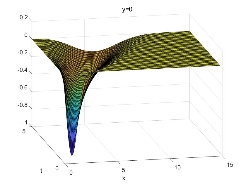
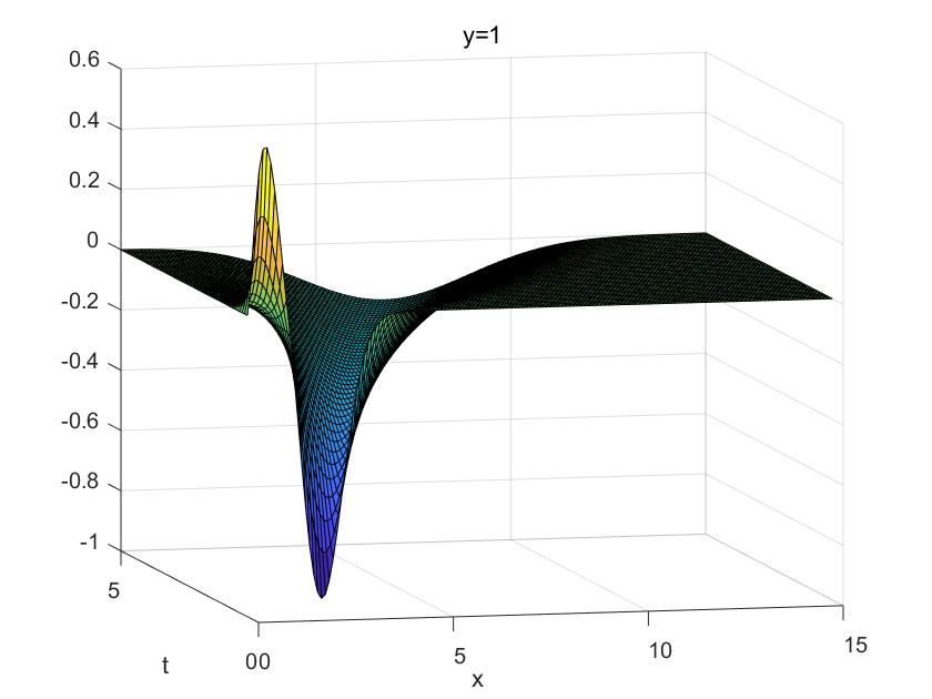
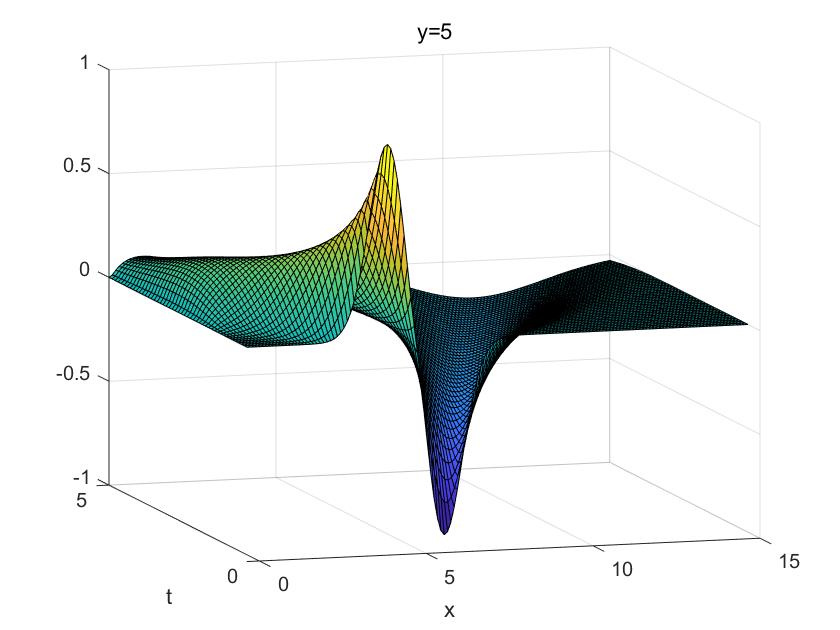
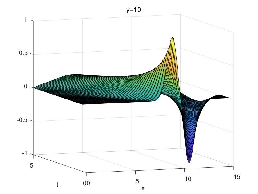
Figure 1: Derivative $\nabla w(t,x)$

Figure 2: Free boundary $s(t)$ for fixed $y>0$ demonstrating feature of “phase transition”

5 Application in Stochastic Optimal Control

In this section, we consider a stochastic optimal control problem related to reflecting diffusion processes. Let

$$X_{t}=x+W_{t}+\int_{0}^{t}u_{s}ds+L_{t}^{u}$$ (5.1)

be a diffusion type process reflecting at zero, where $u$ is adapted and satisfies $|u|_{\infty}\leq\kappa$ on the time interval $\mathbb{R}$. We denote all these controls $u$ as an admissible set $\mathscr{U}$. One problem is to minimize the cost functional

$$J(u)=\mathbb{E}_{x}\left[\int_{0}^{T}f(t,X_{t},u_{t})dt+h(X_{T})\right]$$

by choosing an optimal $u\in\mathscr{U}$. Our interest in this paper is to minimize the following expected discounted cost with infinite horizon:

$$J(u)=\mathbb{E}_{x}\int_{0}^{\infty}e^{-\lambda t}f(X_{t})dt,$$

where we take $T=\infty$, and $h=0$. The problem has been studied in e.g. [3, 10, 12, 23] for diffusion processes with different constraints. Here we consider the case with the reflecting boundary conditions.

Theorem 7.

Let $f(x)$ be of at most polynomial growth, and let

$$v(x)=\inf_{u\in\mathscr{U}}\mathbb{E}_{x}\int_{0}^{\infty}e^{-\lambda t}f(X_{t})dt.$$ (5.2)

Then $v(x)$ is the solution to the ordinary differential equation

$$\frac{1}{2}v^{\prime\prime}+f(x) =\kappa|v^{\prime}|+\lambda v,$$ (5.3)

$$v^{\prime}(0+) =0,$$ (5.4)

on $[0,\infty)$, with at most polynomial growth when $x$ is large enough.

Proof.

The equations (5.3) and (5.4), together with the polynomial growth at infinity, has a unique classical solution $v(x)\in C^{2}([0,\infty))$. Let $V_{u}(x)=\mathbb{E}_{x}\int_{0}^{\infty}e^{-\lambda t}f(X_{t})dt$, we will show that the solution $v(x)=\inf_{u\in\mathscr{U}}V_{u}(x)$. Define the process

$$M_{t}=e^{-\lambda t}v(X_{t})+\int_{0}^{t}e^{-\lambda s}f(X_{s})ds.$$ (5.5)

By Itô formula, we have

$$M_{t} =M_{s}+\int_{s}^{t}e^{-\lambda r}\left(-\lambda v(X_{r})+u_{r}v^{\prime}(X_{r})+\frac{1}{2}v^{\prime\prime}(X_{r})+f(X_{r})\right)dr$$

$$\quad\quad+\int_{s}^{t}e^{-\lambda r}v^{\prime}(X_{r})dW_{r}+\int_{s}^{t}e^{-\lambda r}v^{\prime}(X_{r})dL_{r}^{u},$$

for any $s<t$. Since

$$\quad-\lambda v+u_{r}v^{\prime}+\frac{1}{2}v^{\prime\prime}+f$$

$$\geq-\lambda v+\inf_{u\in\mathscr{U}}(u_{r}v^{\prime})+\frac{1}{2}v^{\prime\prime}+f$$

$$=-\lambda v-\kappa|v^{\prime}|+\frac{1}{2}v^{\prime\prime}+f=0,$$

and the support of $L_{\cdot}^{u}$ is $\{t\geq 0:\ X_{t}=0\}$ a.s., and $v^{\prime}(0+)=0$, so we have

$$M_{t}\geq M_{s}+\int_{s}^{t}e^{-\lambda r}v^{\prime}(X_{r})dW_{r}.$$

Thus,

$$\mathbb{E}_{x}[M_{t}|\mathcal{F}_{s}]\geq M_{s},\quad\textrm{for}\ \forall\ s\leq t.$$ (5.6)

That is, $M_{t}$ is a submartingale. So

$$\mathbb{E}_{x}M_{t}=e^{-\lambda t}\mathbb{E}_{x}v(X_{t})+\mathbb{E}_{x}\int_{0}^{t}e^{-\lambda s}f(X_{s})ds\geq M_{0}=v(x).$$

Let $t\to\infty$, then

$$\mathbb{E}_{x}\int_{0}^{\infty}e^{-\lambda t}f(X_{t})dt\geq v(x),\quad\textrm{for all}\ u\in\mathscr{U}.$$ (5.7)

On the other hand, by taking

$$u_{t}^{*}=-\kappa\mathrm{sgn}(v^{\prime}(X_{t}))\in\mathscr{U},$$ (5.8)

similarly we know that $M_{t}$ is a martingale and $\mathbb{E}_{x}M_{t}=v(x)$ for any $t\geq 0$. So

$$v(x)=\mathbb{E}_{x}\int_{0}^{\infty}e^{-\lambda t}f(X_{t}^{*})dt\geq\inf_{u\in\mathscr{U}}\mathbb{E}_{x}\int_{0}^{\infty}e^{-\lambda t}f(X_{t})dt,$$ (5.9)

where

$$X_{t}^{*}=x+W_{t}+\int_{0}^{t}u_{s}^{*}ds+L_{t}^{u^{*}}.$$

Therefore, we have completed the proof. Besides, we also know that $u^{*}$ is the optimal stochastic control for our problem. ∎

In fact we may obtain the explicit solution for the stochastic optimal control problem by using some simple algebra for the cases where $f(x)=x$ and $f(x)=x^{2}$.

If $f(x)=x$, then we have the value function

$$v(x)=\frac{e^{(\kappa-\sqrt{\kappa^{2}+2\lambda})x}}{\lambda(-\kappa+\sqrt{\kappa^{2}+2\lambda})}+\frac{x}{\lambda}-\frac{\kappa}{\lambda^{2}},\quad\textrm{on}\ [0,\infty).$$ (5.10)

If $f(x)=x^{2}$, the value function $v(x)$ is

$$v(x)=\frac{2\kappa e^{(\kappa-\sqrt{\kappa^{2}+2\lambda})x}}{\lambda^{2}(\kappa-\sqrt{\kappa^{2}+2\lambda})}+\frac{x^{2}}{\lambda}-\frac{2\kappa x}{\lambda^{2}}+\frac{2\kappa^{2}+\lambda}{\lambda^{3}},\quad\textrm{on}\ [0,\infty).$$ (5.11)

Moreover, we may verify that for any $x>0$, $v^{\prime}(x)>0$. Indeed if $f(x)=x$, then

$$v^{\prime}(x)=-\frac{1}{\lambda}e^{(\kappa-\sqrt{\kappa^{2}+2\lambda})x}+\frac{1}{\lambda}=\frac{1}{\lambda}\left(1-e^{(\kappa-\sqrt{\kappa^{2}+2\lambda})x}\right)>0,\quad\textrm{on}\ [0,\infty),$$

and if $f(x)=x^{2}$, then

$$v^{\prime}(x)=\frac{2\kappa}{\lambda^{2}}e^{(\kappa-\sqrt{\kappa^{2}+2\lambda})x}+\frac{2x}{\lambda}-\frac{2\kappa}{\lambda^{2}}.$$

Since the sign of $v^{\prime}(x)$ cannot be seen directly, we look at the second derivative $v^{\prime\prime}(x)$, that is,

$$v^{\prime\prime}(x) =\frac{2\kappa}{\lambda^{2}}(\kappa-\sqrt{\kappa^{2}+2\lambda})e^{(\kappa-\sqrt{\kappa^{2}+2\lambda})x}+\frac{2}{\lambda}$$

$$=\frac{\sqrt{\kappa^{2}+2\lambda}-\kappa}{\lambda^{2}}\left[(\sqrt{\kappa^{2}+2\lambda}+\kappa)-2\kappa e^{(\kappa-\sqrt{\kappa^{2}+2\lambda})x}\right]$$

$$\geq\frac{\sqrt{\kappa^{2}+2\lambda}-\kappa}{\lambda^{2}}\left[2\kappa\left(1-e^{(\kappa-\sqrt{\kappa^{2}+2\lambda})x}\right)\right]>0.$$

Therefore $v^{\prime}(x)>0$ for $x>0$. Thus, we know that the optimal control $u_{t}^{*}$ is the following feedback law by the proof of Theorem 7:

$$u_{t}^{*}=-\kappa\mathrm{sgn}(v^{\prime}(X_{t}))=-\kappa\mathrm{sgn}(X_{t})=-\kappa\in\mathscr{U}.$$ (5.12)

Hence the optimal controlled diffusion process with reflection at zero is then

$$X_{t}=x+W_{t}-\kappa\int_{0}^{t}\mathrm{sgn}(X_{s})ds+L_{t}=x+W_{t}-\kappa t+L_{t}.$$ (5.13)

It is the same process as in (3.7). For this case, we have obtained the explicit form of the transition probability density function $q^{\kappa}(t,x,z)$ of $X_{t}$ in the section §3. That is,

$$q^{\kappa}(t,x,z) =\frac{1}{\sqrt{2\pi t}}\left[e^{-\frac{(x-z-\kappa t)^{2}}{2t}}+e^{-\frac{(x+z+\kappa t)^{2}}{2t}+2\kappa x}\right]$$ (5.14)

$$\quad\quad\quad\quad\quad\quad+2\kappa e^{-2\kappa z}\int_{x+z-\kappa t}^{+\infty}\frac{1}{\sqrt{2\pi t}}e^{-\frac{u^{2}}{2t}}du,$$

for any $x\geq 0$ and $z\geq 0$.

We would like to point out that, for the problems without reflecting barriers, similar formulas have been obtained in [10, 12].

References

• [1] Abate, J., Whitt, W.: A unified framework for numerically inverting Laplace transforms. Informs J. Comput. 18 (2006), no. 4, 408-421.
• [2] Aronson, D.G.: Non-negative solutions of linear parabolic equations. Ann. Scuola Norm. Sup. Pisa (3) 22 (1968), 607-694.
• [3] BeneΕ‘, V.E., Shepp, L.A., Witsenhausen, H.S.: Some solvable stochastic control problems. Stochastics 4 (1980), no. 1, 39-83.
• [4] Borodin, A.N., Salminen, P.: Handbook of Brownian motion-facts and formulae. 2nd ed. Probability and its Applications. BirkhΓ€user Verlag, Basel, 2002.
• [5] Davies, E.B.: Heat Kernels and Spectral Theory. Cambridge Tracts in Mathematics, 92. Cambridge University Press, Cambridge, 1989.
• [6] Fabes, E.B. and Stroock, D. W.: A New Proof of Moser’s Parabolic Harnack Inequality Using the old Ideas of Nash, Arch. for Ratl. Mech. and Anal. 96 (1986), no. 4, 327-338.
• [7] Han, Q., Lin, F.-H.: Nodal sets of solutions of parabolic equations. II. Comm. Pure Appl. Math. 47 (1994), no. 9, 1219-1238.
• [8] Ikeda, N. and Watanabe, S.: Stochastic Differential Equations and Diffusion Processes. Second Edition. North-Holland Math Library, 24. North-Holland/Kodansha, 1989.
• [9] ItΓ΄, K. and McKean, H. P, Jr: Diffusion Processes and their Sample Paths, Second Printing, Corrected. Die Grundlehren der math Wissenschaften, Band 125. Springer-Verlag, Berlin-New York, 1974.
• [10] Karatzas, I. and Shreve, S.E.: Trivariate density of Brownian motion, its local and occupation times, with application to stochastic control. Ann. Probab. 12 (1984), no. 3, 819-828.
• [11] Karatzas, I. and Shreve, S.E.: Connections between optimal stopping and singular stochastic control. II. Reflected follower problems. SIAM J. Control Optim. 23 (1985), no. 3, 433-451.
• [12] Karatzas, I. and Shreve, S.E.: Brownian Motion and Stochastic Calculus. 2 ed. Graduate Texts in Mathematics, 113. Springer-Verlag, New York, 1991.
• [13] Krylov, N.V.: Controlled Diffusion Processes. Stochastic Modelling and Applied Probability, 14. Springer-Verlag, Berlin, 2009.
• [14] LadyΕΎenskaja, O.A., Solonnikov, V.A. and Ural’ceva, N.N.: Linear and Quasi-Linear Equations of Parabolic Type, American Mathematical Society, 1968.
• [15] Lin, F.-H.: Nodal sets of solutions of elliptic and parabolic equations. Comm. Pure Appl. Math. 44 (1991), no. 3, 287-308.
• [16] Mansy, R. and Yor, M.: Aspects of Brownian Motion. Springer-Verlag, Berlin, 2008.
• [17] Nash, J.: Continuity of Solutions of Parabolic and Elliptic Equations, American J. of Mathematics 80 (1958), No. 4, 931-954.
• [18] Norris, J.: Heat kernel asymptotics and the distance function in Lipschitz Riemannian manifolds. Acta Math. 179 (1997), no. 1, 79-103.
• [19] Qian, Z., Russo, F. and Zheng, W.: Comparison theorem and estimates for transition probability densities of diffusion processes. Probab. Theory Related Fields 127 (2003), no. 3, 388-406.
• [20] Qian, Z. and Zheng, W.: Sharp bounds for transition probability densities of a class of diffusions. C. R. Math. Acad. Sci. Paris 335 (2002), no. 11, 953-957.
• [21] Qian, Z. and Zheng, W.: A representation formula for transition probability densities of diffusions and applications. Stochastic Process. Appl. 111 (2004), no. 1, 57–76.
• [22] Revuz, D. and Yor, M.: Continuous Martingales and Brownian Motion. 3 ed. Grundlehren der Mathematischen Wissenschaften, 293. Springer-Verlag, Berlin, 1999.
• [23] Shreve, S.E.: Reflected Brownian motion in the β€œbang-bang” control of Brownian drift. SIAM J. Control Optim. 19 (1981), no. 4, 469-478.
• [24] Skorohod, A.: Stochastic equations for diffusion processes in a bounded region 1, 2, TV $\mathbf{6}$, 264-274 (1961); $\boldsymbol{7}$, 3-23 (1962).
• [25] Stroock, D. W.: Diffusion semigroups corresponding to uniformly elliptic divergence form operators, SΓ©minaire de ProbabilitΓ©s 22 (1988), 316-347.
• [26] Stroock, D.W. and Varadhan, S.R.S.: Multidimensional Diffusion Processes. Grundlehren der Mathematischen Wissenschaften, 233. Springer-Verlag, Berlin-New York, 1979.
• [27] Stroock, D. W. and Varadhan, S. R. S.: Diffusion processes with boundary conditions. Comm. Pure Appl. Math. 24 (1971), 147-225.
• [28] Varadhan, S.R.S.: On the behavior of the fundamental solution of the heat equation with variable coefficients. Comm. Pure Appl. Math. 20 (1967), 431-455.