Evolutionary Models for 15 Galactic Supernova Remnants with New Distances

Abstract

Recent studies using 21 cm HI line and ¹³CO line observations in the inner part of the Galaxy have resulted in new distances for 30 Galactic supernova remnants (SNRs). 15 of those remnants have observed X-ray spectra, for which shocked-gas temperatures and emission measures are measured. Here we apply spherically symmetric SNR evolution models to these 15 remnants to obtain estimates for ages, explosion energies, circum-stellar medium densities and profiles (uniform or wind-type). From the distribution of ages we obtain a supernova birth rate and estimate incompleteness. The energies and densities can be well fit with log-normal distributions. The distribution of explosion energies is very similar to that of SNRs in the Large Magellanic Cloud (LMC), suggesting SN explosions in the LMC and in the Galaxy are very similar. The density distribution has higher mean density for Galactic SNRs than for LMC SNRs, by a factor $\sim$2.5.

1 Introduction

The study of supernova remnants (SNRs) is of great interest in astrophysics (see Vink (2012) and references therein for a recent review). SNRs provide valuable information relevant to stellar evolution, the evolution of the Galaxy and its interstellar medium. SNRs are the dominant source of kinetic energy input into the interstellar medium (Cox, 2005) and thus measuring SNR energetics is critical to understanding the structure of the interstellar medium.

SNRs are observed primarily in X-rays, by emission from hot interior gas with temperature $\sim$1 keV, and in radio, by synchrotron emission from relativistic electrons accelerated by the SNR shockwave. The observational constraints for different SNRs are often different in nature. They depend on the brightness of emissions in different wavebands by a given SNR and by the instruments used to observe that SNR. Only a small fraction of the $\sim$300 observed SNRs in our Galaxy have previously been well enough characterized to determine their evolutionary state, including explosion type, explosion energy and age. A few historical SNR have been observed in great detail and modelled with hydrodynamic simulations. For example, Tycho has been modelled (Badenes et al., 2006) and used to test different models for SN Type Ia explosions. However, most SNRs are not observed nearly as well and have not been subject to similar detailed modelling. For these observationally less-constrained SNRs, it is worthwhile to determine their bulk physical characteristics, but with a simpler approach than full hydrodynamic modelling.

In order to expedite characterization of SNRs, we have developed a set of analytical SNR models for spherically symmetric SNRs and implemented them in Python (Leahy & Williams, 2017). The set of models includes a wide set of models constructed previously by other authors. We carried out the additional step of consistently joining different stages of evolution, which in several cases has not been done before. The resulting models facilitate the process of using different constraints from observations to estimate SNR physical properties of interest.

The current work includes the following. First, we extend the models to calculate the X-ray emission from a SNR during the evolutionary phase between the self-similar ejecta dominated phase and the self-similar Sedov-Taylor phase. Then we solve the inverse problem of how to determine the initial parameters of a SNR using its observed properties. Finally, we apply the solution of the inverse problem to a set of SNRs with newly determined distances. The structure of the paper is as follows. Section 2 presents an overview of the SNR models and the solution of the inverse problem. Section 3 describes the supernova remnant sample and the model fits for individual SNRs. Section 4 present our analysis of the properties of the SNR sample and Section 5 summarizes the results on the distribution of explosion energies and densities.

2 Overview of the Supernova Remnant Evolution

2.1 General SNR Evolution

A SNR is, by definition, the interaction of the SN progenitor’s ejecta with the interstellar medium (ISM) or circumstellar medium (CSM). The various stages of evolution of a SNR include, in order, the ejecta-dominated stage (labelled ED), the adiabatic (or Sedov-Taylor) stage (labelled ST), and radiative stages. These are reviewed in part in many previous publications, including Leahy & Williams (2017), Cioffi et al. (1988), Truelove & McKee (1999) (hereafter TM99) and Vink (2012). The radiative stages are usually divided into the earlier pressure driven snowplow (PDS) stage and later momentum conserving shell (MCS) stage. In addition to these phases, there are the transitions between stages, which we label as ED to ST, ST to PDS, and PDS to MCS, respectively. The ED to ST stage is particularly important, because the SNR is still bright in X-rays and radio, and it is long-lived enough that a significant number of Galactic SNRs could be in this phase. The end of the life of the SNR is usually taken to be when the SNR merges with the ISM, i.e. the shock velocity has dropped to a value similar to the random velocities in the general ISM.

2.2 The Adopted Model for SNRs

For simplicity we assume that the SN ejecta and CSM or ISM are spherically symmetric. The required hydrodynamic equations for a spherically symmetric SNR evolution are summarized by White & Long (1991). The ISM/CSM density profile is taken as a power-law centred on the SN explosion $\rho_{CSM}=\rho_{s}r^{-s}$, with s=0 (constant density medium) or s=2 (stellar wind density profile). The unshocked ejectum is taken to have a power-law density profile $\rho_{ej}\propto r^{-n}$. For these assumptions, the early part of the SNR evolution (the ED phase) follows a self-similar evolution, as determined by Chevalier (1982) and Nadezhin (1985). The SNR shock radius evolution was extended for the ED through ST phases by TM99.

The model for SNR evolution that we construct is partly based on the TM99 analytic solutions, with additional features. A detailed description of the most of the model is given in Leahy & Williams (2017). For example, we used Coulomb collisional electron heating, which is consistent with the results of Ghavamian et al. (2013). However, important extensions have been added in the current work. The main extensions are: i) we calculate the emission measure and emission measure-weighted temperature during the transition from ED phase to ST phase; ii) the inverse problem is solved, which takes as input the SNR observed properties and determines the initial properties of the SNR.

The SNRs modelled here have relatively small physical diameters, thus they are generally in a stage prior to the radiative stage. We checked after obtaining our model results that none of the models had reached the radiative phase, as defined by the time $t_{pds}$ (for example, see TM99). Such non-radiative supernova remnants follow unified evolution (TM99). For the case of uniform ISM, the characteristic radius is $R_{ch}=(M_{ej}/\rho_{0})^{1/3}$ and characteristic time is $t_{ch}=E_{0}^{-1/2}M_{ej}^{5/6}\rho_{0}^{-1/3}$. Here $M_{ej}$ is the mass of ejecta, $E_{0}$ is the explosion energy, $\rho_{0}$ is the mass density of the ISM, $\rho_{0}=\mu_{H}n_{0}m_{H}$, and $n_{0}$ is the hydrogen number density of the ISM. The characteristic velocity is $v_{ch}=R_{ch}/t_{ch}$ and the characteristic shock temperature is $T_{ch}=\frac{3}{16}\mu_{I}\frac{m_{H}}{k_{B}}v_{ch}^{2}$. For the case of a circumstellar wind medium, $\rho\propto r^{-s}$, s=2, the characteristic radius and time are $R_{ch}=(M_{ej}/\rho_{s})$ and $t_{ch}=E_{0}^{-1/2}M_{ej}^{3/2}v_{w}/\dot{M}$. Here $\dot{M}$ and $v_{w}$ are the wind mass loss rate and velocity, yielding $\rho_{s}=\frac{\dot{M}}{4\pi v_{w}}$.

For SNRs which are less than several thousand years old, the post shock gas is a mixture of electrons of lower temperature and different species of ions, each with their own (higher) temperature. The mechanism of electrons heating is taken to be Coulomb collisions. As shown by Leahy & Williams (2017), this electron heating model agrees well with the observed contraints on electron heating (Ghavamian et al., 2013). This allows calculation of the electron temperature as a function of time, so that the X-ray (electron) temperature can be determined in the model.

Element abundances for the ISM/CSM are taken to be solar values, from Grevesse & Sauval (1998). For the SN ejecta, generic abundances values were taken (in units of $log(X/H)+12$) for massive star core-collapse SN as: He: 11.22, C: 9.25, N: 8.62, O: 9.69, Ne: 8.92, Mg: 8.30, Si: 8.79, S: 8.54, Fe: 8.55; and for Type Ia SN as: He: 11.40, C: 12.60, N: 7.50, O: 12.91, Ne: 11.04, Mg: 11.55, Si: 12.75, S: 12.43, Fe: 13.12. The hydrodynamic boundary conditions at the contact discontinuity involve pressure, mass density, velocity and temperature, whereas the EM depends on electron and ion number densities. These are related by $\rho=\mu_{e}m_{H}n_{e}=\mu_{ion}m_{H}n_{ion}$, thus the composition affects the temperature and emission measure of the reverse shock gas. 14 of the 15 SNR in our sample have been previously classified as core-collapse or unknown type. Thus for simplicity, we use the ejecta abundances for core-collapse SN.

The evolution starts with the early ED self-similar phase (valid for $t<t_{core}$ in the notation of TM99). For ejecta with $n>5$ we use the self-similar solutions given by Chevalier (1982). For the current modelling we restrict our calculations to $n>5$ and either $s=0$ (uniform ISM) or $s=2$ (stellar wind CSM).

During the adiabatic (ST) phase valid for $t>t_{rev}$ (using the notation of TM99), the shock radius and shock velocity evolution were calculated using the TM99 solutions. These are much more accurate than the simple Sedov equations, as shown by Leahy & Williams (2017). The reason is that the Sedov models do not include the effect of ejected mass on changing the timescale of evolution.

The transition period from ED phase to ST phase occupies a significant amount of time (TM99). For example, for n=7, the ED phase ends at $t_{cor}=0.363t_{ch}$, the transition phase lasts from $t_{cor}$ to $t_{rev}=2.69t_{ch}$: the transition phase is 7.4 times as long as the self-similar phase. The shock radius and shock velocity during the transition were calculated using the results of TM99.

For the $s=2$ case, the period of self-similar evolution is much longer (e.g., TM99). Thus we only use the self-similar ED phase for $s=2$.

2.2.1 Emission Measures and Temperatures for Ejecta-Dominated, Transition and Adiabatic Phases

The radiation from the SNR post-shock plasma occurs via two body processes, e.g. Raymond et al. (1976). Thus it depends on the emission measure, $EM$, $EM=\int n_{e}(r)n_{H}(r)dV$ with electron density $n_{e}$ and hydrogen density $n_{H}$. $EM$ is measured for a given SNR from its X-ray spectrum, with: $norm=\frac{10^{-14}}{4\pi D^{2}}EM$, with $D$, the distance to the SNR with units in cgs (XSPEC manual at heasarc.gsfc.nasa.gov). The $EM$ is calculated for a given model using the interior density profile of that SNR model. We define the dimensionless $EM$, $dEM$, by

$$dEM=EM/(n_{e,s}n_{H,s}R_{s}^{3})$$ (1)

with $n_{e,s}$ and $n_{H,s}$ the values just inside the shock front. $dEM$ depends only on the profile of the interior density distribution.

The observed temperature of a SNR from the X-ray spectrum is the emission-weighted temperature of the interior gas:

$$T_{EM}=\frac{1}{EM}\int n_{e}(r)n_{H}(r)T(r)dV$$ (2)

We define the dimensionless emission-weighted temperature as the emission-weighted temperature divided by the shock temperature, $T_{s}$: $dT=T_{EM}/T_{s}$. $dT$ depends on the interior profiles of density and of temperature.

We distinguish between forward-shocked (hereafter fs) and reverse-shocked (hereafter rs) interior SNR gas and define the corresponding dimensionless $EM$’s ($dEM_{fs}$ and $dEM_{rs}$) and the dimensionless emission-weighted temperatures ($dT_{fs}$ and $dT_{rs}$). From the observed X-ray spectra it is sometimes clear, based on the observed element abundances, whether the emission is from fs gas or from rs gas. In such cases, the appropriate model emission (fs or rs) is used.

The interior structure ($T(r)$ and $\rho(r)$ at any given time) is required to calculate $dEM_{fs}$, $dEM_{rs}$, $dT_{fs}$ and $dT_{rs}$. $dEM$ and $dT$ are independent of time for the ED and ST self-similar phases of evolution, for which the density profiles have a constant shape. The interior structure solutions for the ED phase for different values of s and n are given by the solutions in Chevalier (1982). We use those solutions to calculate $dEM_{fs}$, $dEM_{rs}$, $dT_{fs}$ and $dT_{rs}$.

The SNR interior structure for the fs gas in the ST phase was calculated using solutions to the hydrodynamic equations carried out by Leahy & Williams (2017). During the ST phase, the fully shocked ejecta has a density profile peaked at the contact discontinuity and is expanding slowly. Cioffi et al. (1988) shows interior density profiles for a SNR with ejecta during the ST phase and later. The ejecta expansion speed at the contact discontinuity (at position $r_{cd}$) is $\sim V_{fs}r_{cd}/R_{fs}$. We carried out numerical solutions to the hydrodynamic equations with ejected mass for the s=0, n=0 case to obtain $dEM_{rs}$ and $dT_{rs}$ in the ST phase.

To calculate $dEM_{fs}$, $dEM_{rs}$, $dT_{fs}$ and $dT_{rs}$ for the ED to ST transition, we used hydrodynamic simulations to obtain the SNR interior profiles. These showed that $dEM$ and $dT$ vary smoothly with time between the ED and ST phases for both fs ISM and rs ejecta. Here we use an interpolation, as a function of $t/t_{ch}$, to obtain the values $dEM$ and $dT$ for transition period between the ED phase and the ST phase. From the hydrodynamic simulations, we find that the interpolation is a good approximation ($\sim 5\%$ error). This is similar to the error in using the TM99 analytic approximations for the shock evolution.

2.2.2 The inverse problem: application of models to SNR data

The forward modelling, taking initial SNR conditions and calculating conditions at time t, is described in Leahy & Williams (2017). The input parameters of the SNR forwardnmodel are time (in yr) plus the following. Ejecta parameters are: energy $E_{0}$; ejected mass $M_{ej}$; ejecta power-law index n; and ejecta composition. The ISM/CSM parameters are: temperature $T_{ISM}$; power-law index s (0 or 2); density $n_{0}$ (if s=0) or mass-loss parameter $\rho_{s}=\frac{\dot{M}}{4\pi v_{w}}$ (if s=2); and ISM/CSM composition. The total number of parameters is 7, taking the composition of ISM/CSM and ejecta to be fixed. For the Galactic SNRs modelled here, we take the ISM/CSM to be solar composition.

For the inverse model, the input parameters are normally the current fs radius, $EM$ and $T_{EM}$. The outer radius of the SNR is the fs radius. $EM$ and $T_{EM}$ are usually dominated by fs emission. However in cases where the element abundances are measured to be enhanced, the emission is dominated by rs ejecta or from a combination of fs ISM and rs ejecta. In some cases both forward and rs emission have been observed as separate components. In these, we fit the dominant component (the one with the higher $EM$, which is normally better constrained observationally) and then check if the other predicted component is consistent with the other observed component.

The model here has more parameters (7) than the number of observed parameters of the SNR (3 if one pair of $EM$ and $T$ is observed or 5 is two pairs are observed). Thus we make further simplifications. $T_{ISM}$ is set to 100K, which doesn’t affect the evolution unless the SNR is very old; and we apply both $s=0$ and $s=2$ models, effectively reducing the number of model parameters to 5. Because s=2 models have much faster growth of the fs radius with time, the two cases give very different parameters, such as age and explosion energy. We normally choose which of the two models yields results most consistent with any other observational data.

• For 3 observed parameters, we normally fix n to be 7 and fix $M_{ej}$, leaving 3 model parameters: age, energy and $n_{0}$ (s=0) or $\rho_{s}$ (s=2). For cases where the SN type is core-collapse (hereafter CC) we take $M_{ej}$=5$M_{\odot}$, and for cases where the SN is Type Ia or unknown, we take $M_{ej}$=1.4$M_{\odot}$.

• For 5 observed parameters, we first fit the dominant emission component. Then we adjust n and $M_{ej}$ to approximately match the $EM$ and $T_{EM}$ of the other component. In effect, there are 5 model parameters : n, $M_{ej}$, age, energy and $n_{0}$ (s=0) or $\rho_{s}$ (s=2).

In summary, some SNRs have 3 inputs: fs radius, and emission measure and temperature of either fs or rs. This results in 3 outputs: age, explosion energy, and either ISM density (for the $s=0$ case) or CSM density parameter (for the $s=2$ case). Some SNRs have 2 additional inputs ($EM$ and $T$ for both fs and rs material), which allows inference of additional constraints on n and $M_{ej}$, resulting in 5 model outputs.

It often not known whether the main emission component is from fs or rs material. In such cases, we apply one model assuming emission from the fs, and one assuming emission from the rs. Because the model calculates $EM$ and $kT$ for both fs and rs, we can determine which model is more consistent with the data. In some cases, both models are consistent. For those cases, other information (e.g. kinematic expansion age) is used to decide which model is more likely correct.

3 The SNR Sample

For the inner Galaxy, a significant number of SNRs (30) have had their distances measured or re-measured using HI absorption and ¹³CO emission data. Details of distance determinations are given in Ranasinghe & Leahy (2017), Ranasinghe & Leahy (2018a), Ranasinghe & Leahy (2018b) and Ranasinghe et al. (2018). Of these, 15 have existing X-ray spectral observations which yield EM and temperature. These SNRs include 2 cases with new distances (no previous values), 9 cases with changed distances and 4 cases with distances confirmed to be the same as from previous studies.

This set of 15 SNRs comprises our sample for modelling. For each SNR, the distance comes from the HI and CO studies and the EM and EM-weighted temperature comes from the X-ray studies. We examined both the VGPS radio images (available for all SNRs) and the Chandra X-ray images (available for some) to measure angular semi-major and semi-minor axes of the outer shock. The average of major and minor axes is used to estimate the average outer shock radius as input to the spherical SNR model. The observational input parameters are summarized in Table 1.

3.1 Models for Individual SNRs in the Sample

3.1.1 G18.1-0.1

G18.1-0.1 was noted as a probable SNR by Odegard (1986) and confirmed as an SNR by Brogan et al. (2006). The distance was determined by Leahy et al. (2014) as 5.6 kpc. That same work analyzed the Chandra X-ray spectrum of G18.1-0.1. Application of a Sedov model gave an age of $\sim$5 kyr and a low explosion energy. The improved distance analysis of Ranasinghe & Leahy (2018a) gave a distance of 6.4$\pm$0.2 kpc, which is used here.

We use the $EM$ and $kT$ from the apec model in Table 2 of Leahy et al. (2014). Our model for uniform ISM (s=0, n=7) for this SNR yields an age of 5400 yr and low explosion energy of 0.19$\times 10^{51}$ erg. For this model, $t_{rev}=3600$ yr and $t_{pds}=9800$ yr so the SNR is in the adiabatic phase. The predicted EM of the rs ejecta is 0.032$\times 10^{58}$cm^-3, much fainter than for the fs. The stellar wind SNR model does not yield a reasonable age (500 yr), so is not used.

3.1.2 G21.5-0.9

G21.5-0.9 consists of a bright central pulsar wind nebula and a faint surrounding shell, thus is CC type. The spin-down age of the pulsar PSR J1833-1034 in G21.5-09 is 4.9 kyr (Gupta et al., 2005). However an expansion speed measurement of the SNR yields an age of 870${}^{+200}_{-150}$ yr Bietenholz & Bartel (2008), making it very young. The distance to this SNR is given by Ranasinghe & Leahy (2018a). The Chandra X-ray image and spectrum was analyzed by Matheson & Safi-Harb (2010). They analyze the extended emission using a two component model consisting of a power-law plus pshock (their Table 4). The power law represents the contribution of synchrotron to the X-ray emission and the pshock represents the gas shocked by the SNR. We use $EM$ and $kT$ from the pshock component from the southern halo (Matheson & Safi-Harb, 2010), and multiply the $EM$ by a factor of two to account for the emission from the northern half of the SNR.

We apply a SNR model for uniform ISM (s=0) with n=7, and 5 $M_{\odot}$ ejecta assuming the fs is providing the X-ray emission. This yields an age of 2450 yr and low explosion energy of 0.019$\times 10^{51}$ erg. For this model, $t_{cor}=3600$ yr so the SNR is in the early ejecta-dominated phase. No consistent models are found for later stages. The predicted EM of the rs is about half of that for the fs and of similar temperature. It would be difficult to distinguish from the fs emission, and thus the model is consistent with a single observed emission component.

Next we apply s=0, rs emission models. The s=0, n=7 model yields an age of 1240 yr, explosion energy of 0.085$\times 10^{51}$ erg and $t_{cor}=1550$ yr. The predicted EM of the fs is nearly the same as for the rs, and the fs has a temperature of 1.1 keV. Alternately, we apply the s=0, rs emission model but with n=9. This yields an age of 470 yr, explosion energy of 0.56$\times 10^{51}$ erg and $t_{cor}=540$ yr. For n=9, the predicted EM of the fs ejecta is one-third of that for the rs and the fs has a temperature of 3.6 keV. The fs component would be difficult to distinguish from the bright PWN emission and the rs emission, so is consistent with observations. Because the s=0 n=9 rs emission model is consistent with the expansion age, we prefer that model over the s=0 fs model and adopt it.

The stellar wind SNR fs and rs models yield unreasonable ages ($\lesssim$200 yr), so are not used.

3.1.3 G21.8-0.6 (also known as Kes 69)

G21.8-0.6 was observed in X-rays with XMM-Newton by Seo & Hui (2013). The VLA radio image and kinematic distance to the SNR are given by Tian & Leahy (2008). The SNR consists of an incomplete radio shell and center-filled X-ray emission. The distance has been updated by Ranasinghe & Leahy (2018a) to 5.6$\pm$0.2 kpc.

The $EM$, $kT$ and uncertainties are from Section 3 and Fig. 3 of Seo & Hui (2013). A consistent SNR model has s=0, n=7, 1.4 $M_{\odot}$ fs emission. This is our adopted model. The SNR is 9700 yr old, in adiabatic stage with $t_{rev}=6200$ yr and $t_{pds}=45000$ yr. The predicted emission measure of the rs ejecta is 0.003$\times 10^{58}$ cm^-3, much fainter than for the fs.

3.1.4 G27.4+0.0 (also known as Kes 73)

G27.4+0.0 is a shell type SNR with an anomalous X-ray pulsar at its center (Helfand et al., 1994; Vasisht & Gotthelf, 1997). The distance of 8.5 kpc was determined by Tian & Leahy (2008). It was observed in X-rays with Chandra and XMM-Newton by Kumar et al. (2014). The X-ray spectrum yielded two components: one with low EM and high kT and a second with high EM and low kT. The first component had solar abundances, so is associated with shocked ISM, and the second had enhanced O, Si and S abundances, so is associated with the ejecta. Borkowski & Reynolds (2017) measured the expansion velocity of the SNR shell as 1100 km/s, assuming distance of 8.5 kpc, and derived a Sedov age of 1800 yr. Ranasinghe & Leahy (2018a) revised the distance to 5.8$\pm$0.3kpc, using a better rotation curve model for the inner Galaxy.

The unabsorbed flux and $kT$ are from Kumar et al. (2014) Table 3 whole “SNR” column values. Their unabsorbed flux was converted to $EM$ using XSPEC with the spectral parameters fixed to their values. We applied a Sedov model using the new distance (and thus radius) obtaining an age of 1600 yr (Table 2), similar to that obtained by Borkowski & Reynolds (2017). However the ST model ignores the effect of ejecta mass, which can considerably affect age and explosion energy estimates.

For this SNR (Kumar et al., 2014), we know the high kT, low EM component is fs emission, and the low kT, high EM component is rs emission. We apply the s=0, n=7, 5 $M_{\odot}$ ejecta, fs emission model to obtain an age of 2160 yr and explosion energy of 0.33$\times 10^{51}$ erg. For this model, $t_{cor}=980$ yr and $t_{rev}=7300$ yr, so the SNR is in the transition between ejecta-dominated and adiabatic phases. However, the predicted EM of the rs is lower (by a factor of $\simeq$0.06) than that for the observed rs component, so is not consistent with observations. For the s=0, n=12, fs emission model, the age reduces to 2020 yr and the explosion energy increases to 0.34$\times 10^{51}$ erg. This model has rs EM increased to 49.2$\times 10^{58}$cm^-3, which now agrees with the rs EM observed, and rs temperature of 0.77 keV. Increasing the ejected mass from 5 to 10 M_⊙ for the s=0, n=12, fs emission model, yields an age increase to 2490 yr, explosion energy decrease to 0.33$\times 10^{51}$ erg, rs EM increase to 52.7$\times 10^{58}$ cm^-3 and rs temperature decrease to 0.51 keV. These values are consistent with the observed values, so this last model is the adopted model.

The stellar wind SNR models for n=7 to 12 yield very low ages (150-200 yr) and very high explosion energies ($\simeq 30-60\times 10^{51}$ erg), so are not used.

3.1.5 G28.6-0.1

G28.6-0.1 was confirmed as an SNR by Ueno et al. (2003) using Chandra observations of the region containing the SNR candidate AX J1843.8-0352, identified by Bamba et al. (2001). The distance to this SNR was obtained by Ranasinghe & Leahy (2018b). The unabsorbed flux and $kT$ are from the Table 2 NEI model of Ueno et al. (2003). Their unabsorbed flux was converted to $EM$ using XSPEC with the spectral parameters fixed to their values.

We apply the s=0, n=7, 1.4 $M_{\odot}$ ejecta, fs emission model. This is the adopted model. This SNR is faint and of large size. It is in a low density region, is relatively old (age $\sim 15,000$ yr) and in the the adiabatic phase ($t_{pds}=101,000$ yr). The model predicted rs emission is very faint (EM of $10^{55}$cm^-3).

The stellar wind s=2 SNR models yield low age ($\sim 1300$ yr) and very high explosion energy $23\times 10^{51}$ erg) so are not used.

3.1.6 G29.7-0.3 (also known as Kes 75)

G29.7-0.3 was identified as a composite SNR by Becker & Helfand (1984). Su et al. (2009) found molecular clouds interacting with the SNR and analyzed the Chandra X-ray spectra of the diffuse shell, away from the central pulsar wind nebula. Their Fig. 8 shows the diffuse X-ray emission from the SNR consists of the SE and SW regions. We use the mean $kT$ from the two spectral fits in their Table 3, and sum the normalizations to determine the $EM$ of the SNR. The first reliable distance of 5.1-7.5 kpc to G29.7-0.3 was given by Leahy & Tian (2008), which was updated by Ranasinghe & Leahy (2018a) to 5.6 kpc.

An s=0 n=7, 5 $M_{\odot}$ ejecta, fs emission model yields an age of 2590 yr and explosion energy of 0.057$\times 10^{51}$ erg. The SNR is in the ED stage, with age just less than $t_{cor}$=2750 yr. The predicted rs emission has EM of 2/3 that of the fs and temperature of 0.33 keV.

An s=0 n=7 rs emission model yields an age of 1650 yr and explosion energy of 0.16$\times 10^{51}$ erg. It is in the transition from ED to adiabatic stage with $t_{cor}$=1520 yr and $t_{rev}$=11300 yr. The predicted fs emission has EM 1.6 times that of the rs and temperature of 1.4 keV, thus is not consistent. However an s=0 n=9 rs emission model yields age of 890 yr and explosion energy of 0.46$\times 10^{51}$ erg. The predicted fs emission has EM 0.37 times that of the rs and temperature of 2.7 keV, so is consistent with the observations.

Stellar wind s=2 SNR models yields low age ($\sim 170$ yr) and high explosion energy $8\times 10^{51}$ erg) so are not used. Because the measured abundances are indicative of rs emission we adopt the s=0, n=9 rs model and use it in Table 4.

3.1.7 G31.9+0.0 (also known as 3C391)

G31.9+0.0 is a mixed morphology SNR (Reynolds & Moffett, 1993) and is interacting with a molecular cloud (Wilner et al., 1998). The distance to G31.9+0.0 is 7.1$\pm$0.4 kpc (Ranasinghe & Leahy, 2017). Sato et al. (2014) carried out a high sensitivity X-ray study of this SNR using Suzaku observations. They determined the X-ray spectral parameters of a two-component plasma in the SNR: a collision-ionization equlibrium (CIE) componnent and a recombining plasma (RP) component. The abundance patterns of the RP are consistent with a core collapse SN. The $kT$ and $VEM$ are from their recombining plasma model (CIE plus NEIJ) Table 3 (third and fourth columns). The $VEM$ was converted to $EM$ using the new SNR distance. The CIE+CIE $kT$ and $VEM$ values are very similar to those for the CIE plus NEIJ model.

Initially we use an ejecta mass of 5 $M_{\odot}$ in our models. An s=0, n=9, fs emission model for the CIE component yields an SN explosion energy of 0.39$\times 10^{51}$ erg, age of 8740 yr and ISM density of 4.53 cm^-3. This model gives rs kT=0.38 keV and EM=0.61$\times 10^{58}$cm^-3. The rs EM is within the observed RP-EM uncertainty range but on the low side and the rs kT is close but lower than the observed RP value. The n=7 and n=12 models give almost the same results as the n=9 model for age, explosion energy and EM, kT for the rs.

The EM of the rs for the s=0, n=9, fs model can be increased by increasing the ejecta mass. For example increasing the ejecta mass to 15 M_⊙ increases the rs EM to 1.9$\times 10^{58}$cm^-3, but lowers the rs kT to 0.26 keV. As a compromise to fitting both EM and kT for the rs we choose the s=0, n=9, 10 M_⊙ model to present in Table 4.

SNR in stellar wind (s=2) models yield much higher EM and lower kT for the rs component compared to the observed RP values, so are not used.

Because this is a mixed-morphology SNR, we apply the WL (White & Long, 1991) model. Our WL model includes Coulomb electron-ion equilibration. We choose an intermediate cloud evaporation parameter ($C/\tau=2$) which has flat interior density and temperature profiles (Fig. 2 of White & Long (1991)), similar to those seen for mixed-morphology SNRs. The WL model does not include any ejecta, but if the SNR is old enough that the emission is dominated by ISM and evaporated cloud emission, the model is a good approximation. The results of the WL model for G31.9+0.0 are given in Table 4. It has nearly the same age and explosion energy as the above adopted model. The WL model has a lower ISM density, as expected, because evaporating clouds contribute to the observed $EM$.

3.1.8 G32.8-0.1 (also known as Kes 78)

G32.8-0.1 is an SNR interacting with a molecular cloud (Zhou & Chen, 2011). The distance was revised to 4.4 kpc by Ranasinghe & Leahy (2018a). The most recent X-ray study of this SNR is presented by Bamba et al. (2016), using Suzaku data. The SNR diffuse emission has an X-ray spectum which was equally well fit with two different two-component models: low (0.63 keV) and high (3.4 keV) temperature VNEI components, or a low temperature VNEI component plus a power-law component. The latter model is preferred by Bamba et al. (2016), and we use $EM$ (converted to the new distance) and $kT$ from that model (their Table 3).

Because there is no clear evidence that this is core-collapse SN, we use an ejected mass of 1.4 M_⊙ and n=7 for modelling. We ran s=0 fs models for different stages of evolution and found a consistent model if the SNR has an age between $t_{cor}$ and $t_{rev}$. The predicted EM of the rs component is 1.4$\times 10^{56}$ cm^-3 in agreement with the EM inferred for the second component of the two-component VNEI model. However the predicted kT for the rs component is a factor of $\sim$10 below the kT of the second VNEI component.

An s=2, n=7 model yields an age of 630 yr and explosion energy of 5.6$\times 10^{51}$ erg, with rs EM 1.0$\times 10^{56}$ cm^-3.

Neither the s=0 nor s=2 models can give a 3-4 keV rs, so we agree with Bamba et al. (2016) that the second component appears more likely to be non-thermal. The low ISM density inferred from the SNR models results from the large size and low EM. This is consistent with G32.8-0.1 interacting with a molecular cloud if the cloud interaction has taken place fairly recently compared to the age of the SNR. The adopted model is the s=0, n=7, 1.4 M_⊙ fs emission model.

3.1.9 G33.6+0.1 (also known as Kes 79)

G33.6+0.1 is a mixed morphology SNR (Rho & Petre, 1998) and a GeV gamma-ray emitter (Auchettl et al., 2014) interacting with a molecular cloud. The distance was revised to 3.5 kpc (Ranasinghe & Leahy, 2018a), significantly closer than previously estimated. The X-ray spectrum was characterized using Suzaku observations (Sato et al., 2016). Two emission components are found, an NEI plasma associated with the rs and a CIE plasma associated with the fs. We use the $EM$ and $kT$ from Table 3 Model B with $EM$ converted to cm^-3 using the new distance. Based on the abundance pattern in the ejecta, Sato et al. (2016) suggest a high mass progenitor of $\sim 40$M_⊙.

We initially used an ejecta mass of $20$ M_⊙ in our models. Consistent s=0 models are all in the evolutionary stage between $t_{cor}$ and $t_{rev}$. The age depends on the ejecta mass with higher ejecta mass yielding older models. E.g. for n=9 models, the age is 8300 yr for $5$ M_⊙ ejecta and 10300 yr for $20$ M_⊙ ejecta. The models produce too high EM for the rs and too low kT compared to measured values, unless the ejecta mass is low, $\simeq$2 M_⊙.

Next we ran s=2 models to fit the fs emission. For the s=2 models, a given n has a fixed ratio of EM of the fs to EM of the rs, independent of ejecta mass. This is a result of the self-similar nature of s=2 models. Thus the observed EM ratio requires n of 6 to 7 with higher n ruled out. For s=2 models, the age is also independent of ejecta mass.

The s=0, n=6 and n=7 models give ages of 3100 yr and 780 yr, respectively. For an ejected mass of 20 M_⊙, these models have explosion energies of 0.48$\times 10^{51}$ erg and 2.93$\times 10^{51}$ erg, respectively. The s=2, n=7 model has rs EM and kT close to the observed values. In Table 4 below we give the parameters for this model. We note that the s=2, n=7 model with 40 M_⊙ ejecta has the same age and rs EM and kT as the 20 M_⊙, but an explosion energy of 8.64$\times 10^{51}$ erg.

3.1.10 G34.7-0.4 (also known as W44)

G34.7-0.4 is a mixed morphology SNR with associated CO emission (Seta et al., 2004; Reach et al., 2005). ASCA spectra determined that the plasma was nearly in CIE (Kawasaki et al., 2005). Uchida et al. (2012) reported the analysis of Suzaku X-ray spectra of W44 demonstrating the presence of a recombining plasma. The X-ray image in 1-2 keV and 2-5 keV bands shows the centre filled nature of the thermal plasma X-ray emission from W44, while the 5-7 keV image shows the hard X-rays are displaced and likely from a different mechanism (Uchida et al., 2012). The abundances of the thermal plasma are mildly enhanced, with Si, S, Ar and Ca all about twice solar. This indicates that the emission is from a mixture of ISM and ejecta. Although the deduced amount of ISM and ejecta contributions depend on rather uncertain ejecta abundances, the low enhancement indicates the emission is likely dominated by ISM emission. The acceptable plasma model from Uchida et al. (2012) is the nonequilibrium ionization jump (NEIJ) model. This model describes a plasma which is in CIE at temperature kT_e1, then has electron temperature dropped suddenly to kT_e2 at some time in the past. The parameter n_et is the product of electron density and time since the temperature was dropped. The cause of the drop is plausibly adiabatic expansion, which would be caused if the blast wave was initially in dense circumstellar environment then propagated into the low density interstellar medium. An estimate of the time since the rapid cooling is $\sim$ 15000 to 20000 yr (Uchida et al., 2012).

We use the combination of regions A, B and C (see their Fig. 1) to represent the emission from the whole SNR. $kT$ is taken as the average of the 3 values of $kT_{e2}$ from their Table 2, and $EM$ is the sum of their $EM$s, converted to the new distance to the SNR. The distance to this SNR was updated by Ranasinghe & Leahy (2018a).

Since most of the SNR blast-wave evolution has occured after the sudden cooling, the appropriate temperature to use for our modelling is kT_e2. We use the sum of the observed emission measures of the different regions to represent the whole SNR emission. We use 5 M_⊙ ejecta, and have verified that for an old SNR, the ejecta mass make very little difference to the model.

The s=0, n=7, fs emission model yields an SN explosion energy of 2.23$\times 10^{51}$ erg, age of 9100 yr, an ISM density of 1.52 cm^-3 and significant rs emission (EM=11$\times 10^{58}$cm^-3), about 7.5% of the EM of the fs.

An s=2, n=7, fs emission model has a low age ($\sim$1400 yr) and high energy (10.2$\times 10^{51}$ erg). The model predicts rs EM and kT of 4.6$\times 10^{59}$cm^-3 and 0.47 keV. This is roughly consistent with it being observed together with the fs emission which has kT = 0.49 keV. The only issues with the s=2 model are the low age and high energy. Thus we adopt the s=0, n=7 model.

Because this is a mixed-morphology SNR, we apply the WL model with $C/\tau=2$. The results of the WL model for G34.7-0.4 are given in Table 4. It has nearly the same age and explosion energy as the above adopted model. The WL model has a lower ISM density, as expected, because evaporating clouds contribute to the observed $EM$.

3.1.11 G39.2-0.3 (also known as 3C396)

G39.2-0.3 is a composite SNR with central pulsar wind nebula and outer shell seen in radio (Patnaik et al., 1990; Anderson & Rudnick, 1993) and X-ray (Becker & Helfand, 1987). Shocked molecular gas has been identified with 3C396 (Hewitt et al., 2009). The updated distance to G39.2-0.3 is 8.5 kpc (Ranasinghe & Leahy, 2018a). Su et al. (2011) carried out X-ray spectroscopy of the thermal X-ray emission from this SNR, detecting two components interpreted as the shocked ISM and the shocked ejecta. Their N and S regions (see their Fig. 9 and Table 2) have enhanced abundances and high $kT$, whereas the E, W and SW regions have near solar abundances and low $kT$. We agree with their interpretation and take the shocked ejecta emission to be N+S ($kT$ and $EM$ from N+S fit). We take the shocked ISM emission to be E+W+SW, and use the $kT$ value of the E region, because it is the same as the mean of the E,W and SW values. We sum the $EM$s of the E, W and SW regions and convert to cm^-3 using the new distance to this SNR.

We apply our SNR models to this CC–type SNR. We model the shocked ISM component first using an s=0, n=9, 5 M_⊙ ejecta, fs emission model. The only consistent solutions are when the SNR is in the transition stage, between $t_{cor}$ and $t_{rev}$. The model yields a predicted rs EM of 4.9$\times 10^{58}$ cm^-3 and rs kT of 0.59 keV. An n=7 fs model yields a rs EM of 1.1$\times 10^{58}$ cm^-3 and kT of 0.68 keV, close to the observed values. An n=6 fs model gives higher rs kT of 0.68 keV, but lower rs EM of 3.2$\times 10^{57}$ cm^-3. The n=7 model as closest to the observations.

A s=2, n=7, fs emission model yields low SNR age (470 yr), high explosion energy (23$\times 10^{51}$ erg) and rs EM and kT very similar to the s=0, n=7 model. Because of the high energy and low age of s=2 models, the s=0, n=7, fs emission model is adopted.

3.1.12 G41.1-0.3 (also known as 3C397)

G41.1-0.3 is a composite SNR and is seen as a shell in radio observations (Anderson & Rudnick, 1993) and as centrally concentrated in X-rays (Rho & Petre, 1998). Safi-Harb et al. (2005) presents the Chandra X-ray study of this SNR. The spectral fitting for the diffuse emission of the bright and large Eastern and Western Lobe regions (see Fig. 6 and Table 3) was used to represent the spectrum of the whole SNR. $kT$ was taken from the Western Lobe, because that is equal to the mean of the two Lobes and better represents the uncertainty. $EM$ was taken as the sum of Eastern and Western lobes, multiplied by 2 to account for the missing diffuse emission (see their Fig. 6), then converted to cm^-3 using the new distance of the SNR. Based on the ejecta abundances, G41.1-0.3 was identified to be a Type Ia remnant with an energetic explosion (Yamaguchi et al., 2015). A new distance was obtained and modelling of this SNR was carried out by Leahy & Ranasinghe (2016). That gave a low age and confirmed an energetic explosion. The updated distance to G41.1-0.3 is 8.5 kpc (Ranasinghe & Leahy, 2018a).

Because it is type Ia, we apply s=0, 1.4 M_⊙ ejecta models using the type Ia ejecta compositions given in Section 2.2. We find consistent models for ages $>t_{rev}$. The model with n=7 predicts EM of the rs to be 0.19$\times 10^{58}$ cm^-3 closer to the observed values than for other values of n. The model gives kT of the rs as 6.0 keV. This could be a result of our assumption of uniformly mixed ejecta composition. For example, if we instead use typical CC ejecta composition which has lower mean ion mass, the rs temperature is 2 keV. Fitting the ejecta composition would likely allow fitting the rs EM and T. However that is a complex procedure beyond the scope of the current work.

A stellar wind SNR model (s=2, n=7) yields a lower age (1300 yr) and explosion energy of 0.95$\times 10^{51}$ erg. The predicted EM and kT of the rs are 3.0$\times 10^{57}$ cm^-3 and 0.43 keV. In this case the EM is close to the observed value but the temperature is low. Adjusting the ejecta composition could likely give a temperature closer to the observed value. The s=2, n=7 model has explosion energy consistent with that deduced by (Yamaguchi et al., 2015). Thus the adopted model is the s=2, n=7 one.

3.1.13 G43.3-0.2 (also known as W49B)

G43.3-0.2 is a mixed morphology SNR (Rho & Petre, 1998). The X-ray spectrum was shown to consist of a solar abundance component and a heavy element enriched component (Hwang et al., 2000), and noted as a probable type Ia SNR. G43.3-0.2 was discovered to have a recombining plasma by Kawasaki et al. (2005). With a long Suzaku observation, the integrated X-ray spectrum of G43.3 was analyzed by Ozawa et al. (2009). This confirmed the presence of a recombining plasma. Because this analysis gives the spatially integrated X-ray spectrum, we use their parameters for $kT$ and $EM$ for the whole SNR found using the CIE model (see their Table 1 and Section 4.4), with their $VEM$ converted to cm^-3 using the newest distance to the SNR . Lopez et al. (2013) illlustrate its unusual X-ray morphology (their Fig.3), with an iron-rich bar. They analyze Chandra X-ray spectra of $\sim$700 small regions, and conclude that G43.3-0.2 likely originates in a jet-driven core-collapse explosion, rather than a type Ia. Because of the conflicting evidence for type Ia or CC, we take the SN type of G43.3-0.2 as unknown. Further analysis by Lopez et al. (2013b) found that the origin of the recombining plasma was likely adiabatic expansion of the hot plasma. The updated distance to G43.3-0.2 is 11.3 kpc (Ranasinghe & Leahy, 2018a).

We apply models with ejecta masses of 1.4 M_⊙ for a type Ia explosion and 5 or 10 M_⊙ for a CC explosion. The observed abundance of Fe and Ni are $\simeq$ 5 times solar, but the large shock radius and large $EM$ imply the emission is dominated by swept up ISM. The iron abundance is elevated (5 times solar) but it is not clear if it is dominated by ISM or ejecta emission. The swept up mass for W49B is estimated as $(4\pi/3)~{}n_{0}~{}R^{3}~{}\simeq~{}80~{}M_{\odot}$, using an estimated $n_{0}=1$ cm^-3. An iron rich ejecta of $\sim 1~{}M_{\odot}$, would yield the observed abundance enhancement, so the emission is mostly from the ISM. Thus we apply fs models.

The s=0, n=7, 9 or 12, and 1.4 or 5 M_⊙ ejecta models all have age larger than $t_{rev}$. The age is 3240-3250 yr for the 1.4 M_⊙ ejecta cases, and 3400-3430 yr for the 5 M_⊙ ejecta cases. The predicted rs $EM$ is small enough (1% of fs EM for 5 M_⊙, and 5% of fs EM for 1.4 M_⊙) to be consistent with the observed X-ray spectra, which is dominated by fs EM. The high predicted rs $kT$ ($\simeq$2.8 keV for 5 M_⊙ ejecta, $\simeq$7.8 keV for 1.4 M_⊙ ejecta) might be related to the observed recombining plasma in this SNR (see Section 4.3 below).

The s=0, n=7, 9 or 12 with 10 M_⊙ ejecta models evolve more slowly, so they are in the stage $t_{cor}<t<t_{rev}$. However these models all have the rs emission with EM $\sim$5 times larger than the fs, so are not consistent with observations.

For a SNR in a stellar wind (s=2) with 1.4 M_⊙ ejecta, the n=7 model has the fs emission brighter than the rs, but higher n models have the rs brighter so that they are inconsistent with the observations. However, for all n, they require high explosion energies (0.6 to 5$\times 10^{53}$ erg) and yield low ages (290 to 690 yr). For a SNR in a stellar wind (s=2) with 5 or 10 M_⊙ ejecta the ages and rs $EM$s are similar to the 1.4 M_⊙ ejecta, but the explosion energies are $\simeq$3 (for 5 M_⊙ case) and $\simeq$6 (for 10 M_⊙ case) times larger. Thus the s=2 models are not realistic.

Only the s=0, n=7, 9 or 12, and 1.4 or 5 M_⊙ ejecta models are consistent with observations. We have a preference for the s=0, n=7, 1.4 M_⊙ model because of the elevated iron abundance but not intermediate mass elements. This is characteristic of type Ia explosions, and we adopt that model.

Because this is a mixed-morphology SNR, we apply the WL model with $C/\tau=2$. The results of the WL model for G43.3-0.2 are given in Table 4. It has nearly the same age and explosion energy as the above adopted model. The WL model has a lower ISM density, as expected, because evaporating clouds contribute to the observed $EM$.

3.1.14 G49.2-0.7 (also known as W51C)

G49.2-0.7 is part of the W51 complex containing prominent HII regions W51A and W51B. and has been detected in $\gamma$-rays (Abdo et al., 2009). The HI absorption spectrum was analyzed by Tian & Leahy (2013), who found that G49.2-0.7 is this side of the tangent point and not associated with high velocity HI. The radio emission of the SNR was modelled using magneto-hydrodynamic simulations by Zhang et al. (2017), yielding a new angular diameter and giving an estimate of the ejecta mass as 11M_⊙. Here we use an angular radius for the SNR of 21 arcminutes, based on comparison of the radio image with the magneto-hydrodynamic simulations. The SNR distance was updated to 5.6 kpc by Ranasinghe & Leahy (2018a).

G49.2-0.7 has been studied a number of times in X-rays, including an analysis of Chandra observations by Koo et al. (2005), Hanabata et al. (2013) analyze Suzaku observations of the diffuse thermal X-ray emission of G49.1-0.7 and find it is best fit with an NEI model. There is an additional hard X-ray component associated with the overlap of the SNR and adacent molecular clouds, which is not well understood but could be associated with synchrotron X-rays from TeV electrons. Sasaki et al. (2014) analyze XMM-Newton observations of the SNR and final similar results in their spectral analysis but suggest that the hard component originates in a pulsar wind nebula. They note that their extended region 1 (south-eastern half of the SNR) has solar abundances but their region 2 (the western half) has enhanced Ne and Mg abundances, and infer a progenitor mass of $\gtrsim$20M_⊙.

We model the thermal component here and use the spectral parameters given in Table 2 of Hanabata et al. (2013) for the NEI model fits for Regions 1 and 2 combined. The $kT$ for Regions 1 and 2 are nearly identical, so we use that for Region 1. We sum the $EM$ values of Regions 1 and 2, which contain most of the 0.5-2.5 keV flux from the SNR (see their Fig. 2), then convert the sum to cm^-3 using the newest distance to this SNR.

We first apply s=0, 10 M_⊙ ejecta, fs emission models. For for different n, these are all in the stage with $t_{core}<t<t_{rev}$. The n=7 model produces fs emission much higher than for the rs, so is not consistent with observation of enhanced Ne and Mg abundances. n=9 to 12 models produce similar $EM$ and $kT$ for fs and rs.

We next apply s=0, 10 M_⊙ ejecta, rs emission models. These produce results consistent with the fs emission models. I.e. the n=7 model produces fs emission much higher than for the rs, so is not consistent with observations. n=9 to 12 models produce similar $EM$ and $kT$ for fs and rs.

It is likely that the observed X-ray emission has contributions from both forward and rs emission. Thus the models support the suggestion by Sasaki et al. (2014) that their region 1 is shocked ISM and their region 2 is shocked ejecta. The best matching fs emission model with 10 M_⊙ ejecta has n=9. For this model the age is 16000 yr, the explosion energy is 0.76$\times 10^{51}$ erg and ISM density is 0.021 cm^-3. The fs and rs temperatures are nearly the same (0.70 and 0.61 keV) and the fs and rs each contribute half of the observed emission measure. The s=0, n=9, fs emission model is the adopted model.

We calculated an s=0, n=9, fs emission model with 20 M_⊙ ejecta because of the high suggested progenitor mass. The age is 18000 yr, the explosion energy is 0.73$\times 10^{51}$ erg and the ISM density is 0.020 cm^-3, not much different than the adopted model. For all of our models the ISM density is low. G49.1-0.7 has expanded into a low density medium prior to colliding with the molecular cloud on its western side (e.g. see Fig. 1 of Koo et al. 2005).

Stellar wind SNR models (s=2) require large energies ($\sim$ 2$\times 10^{52}$ erg) and low ages ($\sim$3000 yr), so are considered unlikely.

3.1.15 G54.1-0.3

G54.1-0.3 is a Crab-like SNR (Lu et al., 2002) with the central region dominated by non-thermal X-ray emission. Based on the pulsar spin-down age of 2900 yr, the SNR age is estimated at 1500-6000 yr (Camilo et al., 2002). Bocchino et al. (2010) use XMM-Newton and Suzaku observations of G54.1-0.3 to detect the thermal emission in the faint outer regions of the SNR. They corrected for scattering of the bright central PWN emission into the outer shell region of the SNR. We use the spectral parameters from their fit to the SNR shell spectrum, in their Table 2, and use XSPEC to convert their unabsorbed flux for the shell into XSPEC norm, then into $EM$ using the new distance to the SNR. The SNR distance was first determined by Leahy et al. (2008), then updated to 4.9 kpc by Ranasinghe & Leahy (2018a).

This is a core-collapse SNR with central PWN, so we use an ejecta mass of 5 M_⊙. s=0 models for both fs emission and rs emission are all in the stage with $t_{core}<t<t_{rev}$.

The s=0, n=7, fs emission model gives age of 2200 yr and explosion energy of 0.63$\times 10^{51}$ erg. The s=0, n=9, fs emission model gives age 2500 yr and explosion energy 0.48$\times 10^{51}$ erg, but has the $EM$ of the rs larger than for the fs, so is not consistent.

The s=0, n=7, rs emission model has age of 1600 yr and explosion energy of 1.39$\times 10^{51}$ erg, but has $EM$ of the fs larger than for the rs, so is not consistent. The s=0, n=9, rs emission model has age of 880 yr and explosion energy of 3.43$\times 10^{51}$ erg. This model has $EM$ of the fs smaller than for the rs, so is consistent. The s=0, n=12, rs emission model has a low age (600 yr) and a large explosion energy (6.1$\times 10^{51}$ erg) so is considered less likely.

s=2 models require large energies ($\sim$ 2$\times 10^{52}$ erg) and low ages ($\sim$360 yr), so are considered unlikely. Thus either s=0, n=7 fs emission or s=0, n=9 rs emission are consistent with the X-ray observations. We have a preference for the fs emission model based on the consistency with the pulsar spin-down age, so we adopt that one.

4 Results and Discussion

4.1 Comparison with Analytic ST Models

We have applied our SNR model (extension of the TM models) to our SNR sample. For comparision, we apply simpler ST models to find the corresponding Sedov age, ISM density and explosion energy parameters. One procedure is to assume an explosion energy and ISM density to determine Sedov ages using the ST equations, e.g from Cox (1972). Another approach is to use a model emission measure to derive density, then apply the ST equations to derive explosion energy and age from density and outer shock radius. The latter method is used here.

We compare two ST model calculations: one (commonly used) method uses a simple model emission measure and electron temperature equal to shock temperature (called simple model); and the second uses emission measure and temperature profiles from the ST hydrodyamic solution combined with the Coulomb electron heating formalism (called electron heating model). The simple model emission measure used is $dEM$=1. The electron heating model is similar to that used for the Sedov model of Hughes et al. (1998) (their Section 3.2), although our model is simplified in the following way. The electron heating model used here is self-similar, so we omit non-equilibrium ionization, which breaks self-similarity. Electron heating is more important for SNR dynamics than non-equlibrium ionization (e.g. Ghavamian et al. (2013)), although non-equlibrium ionization is important for radiative losses, and for deriving electron temperatures from observed X-ray spectra. The electron temperatures used here (in Table 1) are from X-ray spectral models which include non-equilibrium ionization. For the SNRs here, the ages are low enough that radiative losses are not important, so non-equlibrium ionization effects on the SNR models is expected to be small.

We show our calculated results from both ST models in Table 2 using the input $EM$ and $kT$ and radius values from Table 1. Consistent with the conclusion of Hughes et al. (1998), we find the observed electron temperature corresponds to a higher ion temperature in the electron heating models. This implies a higher shock speed and thus a younger age for the electron heating models. Partially compensating for this is a second effect: the simple model takes the observed electron temperature to be the shock temperature; but the electron-heating model uses the average over the entire shocked gas in the SNR, which is hotter than the shock temperature. This leads to a lower inferred shock temperature in the electron heating model for a given observed temperature. Thus older or higher density SNRs, where electron heating has time to equilibrate electron-ion temperatures, have a lower inferred shock speeds and increased ages.

The SNR radius and ISM density yield age and explosion energy from the ST formulae. The ST solution assumes an ejected mass of zero and thus the emission is 100% from the forward-shocked ISM. In cases where the assumptions of the ST model are approximately valid, i.e. for older SNRs, the ST parameters are close (within $\sim 10\%$) to those from the more complete models here. Often, some of the assumptions of the simple ST model are strongly violated. For example, the observed emission can have a significant rs component, the ejecta mass can be large enough to strongly affect the evolution, or the explosion can be in stellar wind environment instead of a uniform ISM. For those cases that the ST assumptions are not valid, we find the Sedov age, ISM density and explosion energy parameters are often very different from those found using the more complete model that we have used here. This demonstrates the need for using a more physically realistic model than the ST model.

4.2 Comparison of TM with numerical ST model

For validation, we compare our extended TM model results with results from another sophisticated model for the same set of SNRs. A set of 7 SNRs in the Large Magellanic Cloud has been modelled using a numerically integrated Sedov model by Hughes et al. (1998), and by Leahy (2017) using the TM model. Hughes et al. (1998) used a Sedov temperature and emissivity profile, and integrated the non-equilibrium ionization equations for sets of parameters to fit ASCA spectra of the SNRs. This was done for two cases (equal electron-ion temperatures and Coulomb equilibration of electrons with ions). Leahy (2017) used the TM (s=0, n=7) shock evolution model, with a fixed ejecta mass of 1.4 M_⊙. The input data for the two models were different. Hughes et al. (1998) used ASCA data from 1993-1995, whereas Leahy (2017) used higher quality XMM-Newton results (Maggi et al., 2016) from 2001-2015 and updated values of SNR radius.

The model values of $E_{0}$, $n_{0}$ and age from the two studies are compared in Table 3. It is seen that the input SNR radius is quite different for the two studies, especially for SNR N23. In order to compensate for this, our TM model was applied to these SNRs using the XMM-Newton $kT$ and $EM$ values but radius values from Hughes et al. (1998). Those results are labelled as (L2) in Table 3 are much closer to the Hughes et al. (1998) model values for most cases. This shows that the radius difference was the main cause for the differences in derived parameters. Another cause of the parameter differences is the difference in SNR spectra observed by ASCA and XMM-Newton. Overall, the comparison shows that the Hughes et al. (1998) model and current model produce similar results for the same SNRs.

4.3 Comments on SNRs in Non-uniform Media

Three of the SNRs above are mixed morphology (MM) SNRs: 3C391 (G31.9+0.0), W44 (G34.7-0.4), and W49B (G43.3-0.2). A model proposed for mixed morphology SNRs is the self-similar White and Long(WL) model for a SNR in a cloudy ISM (White & Long, 1991). This model assumes zero mass of ejecta, but can be a good approximation to MM SNRs if the age is large enough that the X-ray emission is dominated by shocked ISM and evaporating clouds compared to ejecta. 3C391 has EM dominated by shocked ISM. W44 has a slight enhancement of Si, S, Ar and Ca abundances so its emission is mainly ISM with a small contribution ($\sim$1%) from ejecta. W49B has higher iron abundance (5 times solar) but the emission is still mostly from the ISM (see estimate of swept-up mass in Section 3.1.13). Thus the WL model should be a reasonably good approximation for these three SNRs. Table 4 shows the results of applying the WL model to MM SNRs. The derived ages and explosion energies are the same as for the TM model, supporting the TM model results. The WL model densities, which are intercloud densities, are lower than the TM model densities, which represent mean densities, by a factor of $\simeq$0.57 for all 3 MM SNRs.

These same MM SNRs have a detected recombining plasma (RP). The origin of RP in SNRs is not yet well understood. There are two proposed explanations: the rarefaction model in which shocked material breaks out from dense circumstellar medium into rarefied interstellar medium (Shimizu et al., 2012), and the thermal conduction model in which evaporating dense material rapidly cools shocked plasma (Zhou et al., 2011). The latter is more consistent with the fact that MM SNRs are associated with detections of RP. This also indicates that the WL models are likely a better approximation than the TM models for MM SNRs.

We applied both uniform ISM (s=0) and stellar wind (s=2) SNR models to each SNR. There was an expectation that a significant fraction of the SNRs would better be described by the s=2 models. CC SNR have different types of progenitors. Smith et al. (2011) (Fig. 1) give the fractions of SN types. To obtain consistency with stellar evolution, Smith et al. (2011) argue that binary evolution is important and they give possible scenarios. We adopt their favored scenario (their Fig. 7), which has the following SN progenitors. 48.2% are type II-P with initial mass 8.5-18.7 M_⊙. 6.4% are type II-L with initial mass 18.7-23.1 M_⊙. 8.8% are type II-n with initial mass above 23.1 M_⊙. 27.7% are type IIb + Ibc with initial mass above 8.5 M_⊙. 8.8% are type Ic with initial mass above 23.1 M_⊙. The type II-P, II-L and II-n (total of 63.4% of SN) retain their hydrogen envelopes. The other types are stripped-envelope SN via stellar winds, LBV eruptions, or Roche-lobe overflow in binary systems. A high fraction of the stellar wind systems and some fraction of the LBV and Roche-lobe systems are expected to have an s=2 like circumstellar environment. This leads to the expectation that $\sim$20-40% of CC SNR would be described by s=2 SNR models. For type Ia SNR, single degenerate models are expected to have s=2, caused by the system mass-loss wind of the accreting white dwarf. If the type Ia is caused by a double degenerate system, no wind is expected so s=0 is expected.

We find that only 2 of the 15 SNRs are best described by an s=2 model. One of these is type Ia and the other is CC type. The 6 unknown types in the sample (Table 1) are all fit best with an s=0 model. Among those, there are likely one or two type Ia based on type Ia and CC SN frequencies (van den Bergh & Tammann, 1991). Those could be double degenerate type Ia SNR, thus consistent with s=0. We find 7 of 8 confirmed CC type SNR are s=0 SNR. Most massive stars, above $\sim$23 M_⊙ as noted above, are expected to have a stellar wind, resulting in s=2 SNR. A significant fraction of massive stars are in binaries, where the interaction between the stars can complicate the circumstellar density profile. Many massive stars are in stellar clusters where winds from nearby (fractions of a pc) massive stars can interact with the wind of the progenitor and produce complex structures in the ISM which may be better represented by a uniform density than a stellar wind profile. Unless we are ready to accept the high explosion energies ($\sim 10^{53}$ erg) and low ages (few hundred yr) for the majority of s=2 models, the current results are telling us that s=2 wind profiles are more rare than expected: $\sim$15% compared to $\sim$20-40% .

There are uncertainties introduced by applying spherically symmetric (SS) models to SNRs, because SNRs are observed to be non-symmetric. One measure of departure from SS is the departure of the major-axis to minor-axis ratio, $r_{axes}$ from 1. For the SNRs in our sample, $r_{axes}$ has a range from 1.0 to 2.07, a mean of 1.32 and standard deviation of 0.32. The most non-circular SNRs are G29.7-0.3, G32.8-0.1 and G41.1-0.3. G29.7-0.3 (Su et al., 2009) and G32.8-0.1 (Zhou & Chen, 2011) are interacting with molecular clouds and are X-ray and radio bright on one side. G41.1-0.3 (Safi-Harb et al., 2005) is elongated so has an asymmetric environment but has not been confirmed to be interacting with molecular cloud (Ranasinghe & Leahy, 2018a). The departures from SS for non-symmetric SNRs will affect their evolution, and parameters determined by applying SS SNR models will be approximations.

Existing SNR models are SS, so they cannot be used to determine the errors in using SS models for non-symmetric SNRs. Leahy & Williams (2017) review analytic models for SNRs, which are all SS. Hughes et al. (1998) and Borkowski et al. (2001) develop the numerical implementation of the ST model, which is SS, and include non-equilibrium ionization for calculation of synthetic X-ray spectra. Badenes et al. (2006), and references therein, apply SS hydrodynamic SNR models with ejecta, combined with calculation of synthetic X-ray spectra to model X-ray observations.

Two possible ways of estimating errors in using SS models for non-symmetric SNRs are as follows. One method is to analyze a non-symmetric SNR in angular sectors, applying a different SS model to each sector. This assumes that the properties in a given sector do not affect those in neighboring sectors. Then one can test if the derived SNR properties differ by sector, and whether the summed properties from the sectors are consistent with those derived from a single SS model applied to the whole SNR. For example, one sector of an SNR expanding into a high density region or molecular cloud could be approximated by having a high density model for that sector. A second method is to create idealized asymmetric density distributions, and parametrize these in order to have a manageable set of models. Then one can calculate the resulting SNR structure using a hydrodynamic code, and calculate the resulting X-ray spectrum and image. Finally one can fit the spectrum and image to data to obtain model parameters to compare to SS model parameters. These are goals for future work.

4.4 Estimated SNR Population Properties

The summary of our adopted models for the 15 SNRs is presented in Table 4. The statistical properties of the ages, explosion energies and ISM densities of the SNR sample are now examined. A similar analysis was carried out for the LMC SNR population by Leahy (2017). For that sample of 50 SNRs the observations are much closer to complete. The current sample is limited to the part of the Galaxy covered by the VGPS survey and limited to SNRs with adequate X-ray spectra. The volume of the Galaxy covered by the VGPS and by the X-ray observations is not easy to determine, partly because of confusion limits and partly because of sensitivity limits, both in the presence of a variable background. For X-ray measurements, SNRs which are further from the Sun suffer more from absorption by Galactic foreground material. One crude approximation of the fraction of the Galaxy observed in the current sample is the VGPS longitude range (18^∘ to 67^∘) divided by the full range of 360^∘, or 0.136. This ignores missing SNRs which are at higher latitudes (the VGPS maximum latitude varies from 1.3 to 1.9^∘), but also ignores the concentration of SNRs towards smaller longitudes ($\sim 270^{\circ}$ to $360^{\circ}$ and $0^{\circ}$ to $\sim 90^{\circ}$). We compare to Green’s catalog (Green, 2017), which lists 295 Galactic SNRs. 49 of these are in the VGPS survey area, yielding a fraction of 0.166, similar to the estimate above.

The model ages give information on the SN birth rate, subject to the uncertainties of the incompleteness of the sample. Fig. 1 show the cumulative distribution of model ages for our sample of 15 SNRs. The straight lines are the expected distributions for constant birth rates of 1 per 300 yr and 1 per 700 yr, respectively. The 1 per 300 yr line fits well the SNRs with the smallest 3 ages and the 1 per 700 yr line fits approximately the SNRs with the 10 lowest ages. This can be interpreted as increasing incompleteness of the sample for older SNRs. This is expected, as young SNRs are brighter and more easily measured to have an X-ray spectrum. The expected SNR birth rate in the Galaxy is 1 per 40$\pm 10$ yr (Tammann et al., 1994), with rates per SN type (Ia, Ib and II) discussed by van den Bergh & Tammann (1991) (see Table 11 in that paper). Using the fraction above of the fraction of 0.166 of Galactic SNRs in the sample region this translates to 1/(200 yr) to 1/(300 yr) for the sample region. This is close to the 1/(300 yr) birth rate estimate shown in Fig. 1 for the youngest SNRs (age $<$1000 yr). The agreement suggests that the X-ray detections are near 100% for the youngest SNRs. It also suggests that the decreasing birth rate with increasing age seen in Fig. 1 is caused by increasing incompleteness of X-ray (and perhaps radio) detections for older SNRs. I.e. for ages $\lesssim$5000 yr the incompleteness is a factor $\sim$2, yielding half the expected birth rate. The incompleteness continues to increase for higher ages, reaching a factor $\sim$4 for the oldest SNRs ($\sim$15000 yr) in the sample .

The cumulative distribution of explosion energies is shown in Fig. 2. This distribution is not consistent with uniform or Gaussian distributions, but is consistent with a log-normal distribution. The property that SNR explosion energies follows a log-normal distribution was discovered by Leahy (2017). The solid line in Fig. 2 is the best fit cumulative distribution, with parameters $E_{av}=5.4\times 10^{50}$ erg and $\sigma_{logE}$=0.45, which corresponds to a 1-$\sigma$ dispersion factor of 1.9 in energy. These parameters are similar to as those derived from the LMC SNR sample of $E_{av}=5.4\times 10^{50}$erg and $\sigma_{logE}$=0.47 (Leahy, 2017). This suggests that the LMC and Galactic SNR samples are very similar, and thus LMC and Galactic SN are very similar.

The cumulative distribution of ISM densities is shown in Fig. 3 for the 13 of the 15 SNRs with a derived ISM density. This distribution is consistent with a log-normal distribution. The property that ISM densities in the neighborhood of SN explosions has a log-normal distribution was first shown by Leahy (2017). The best fit cumulative distribution is shown by the solid line in Fig. 3. The parameters are $n_{0,av}=0.26$ cm^-3 and $\sigma_{log(n_{0})}$=0.80, which corresponds to a 1-$\sigma$ dispersion factor of 6.3 in density. For the LMC SNR sample (Leahy, 2017), the mean density was considerably lower, $n_{0,av}=0.08$ cm^-3 and the dispersion similar. The difference in mean density is not surprising because the current sample is mainly SNRs in the inner Galaxy whereas the LMC sample was for the whole LMC.

5 Conclusion

Distances to Galactic SNRs have improved significantly, allowing determination of radii and enabling the application of SNR models. We extended spherically symmetric SNR evolution models to include effects of ejecta mass and emission from shocked ejecta. We applied the models to estimate SNR parameters for our sample of SNRs from the inner Galaxy. Then we examined the distributions of the parameters to determine properties of the Galactic SNR population in the inner Galaxy. The estimated birth rate is consistent with estimates of the overall Galactic SNR birth rate and with estimates of the fraction of SNRs in the Galaxy in our sample. We find that the energies and ISM densities of SNR can be well fit with log-normal distributions. The distribution of explosion energies is very similar to that for SNRs in the Large Magellanic Cloud (LMC), suggesting a surprisingly close similarity in the population of SN explosions in the LMC and in the Galaxy. The ISM density distributions for Galactic and LMC SNRs have similar dispersion but Galactic SNRs have a higher mean density by factor $\sim 2.5$. A higher mean density is expected because our sample SNRs are selected from the inner Galaxy.

In future, we plan to extend this type of study of SNRs to include all Galactic SNRs with measured distances. The goal is to significantly increase the sample size and better determine the intrinsic properties of SNRs.

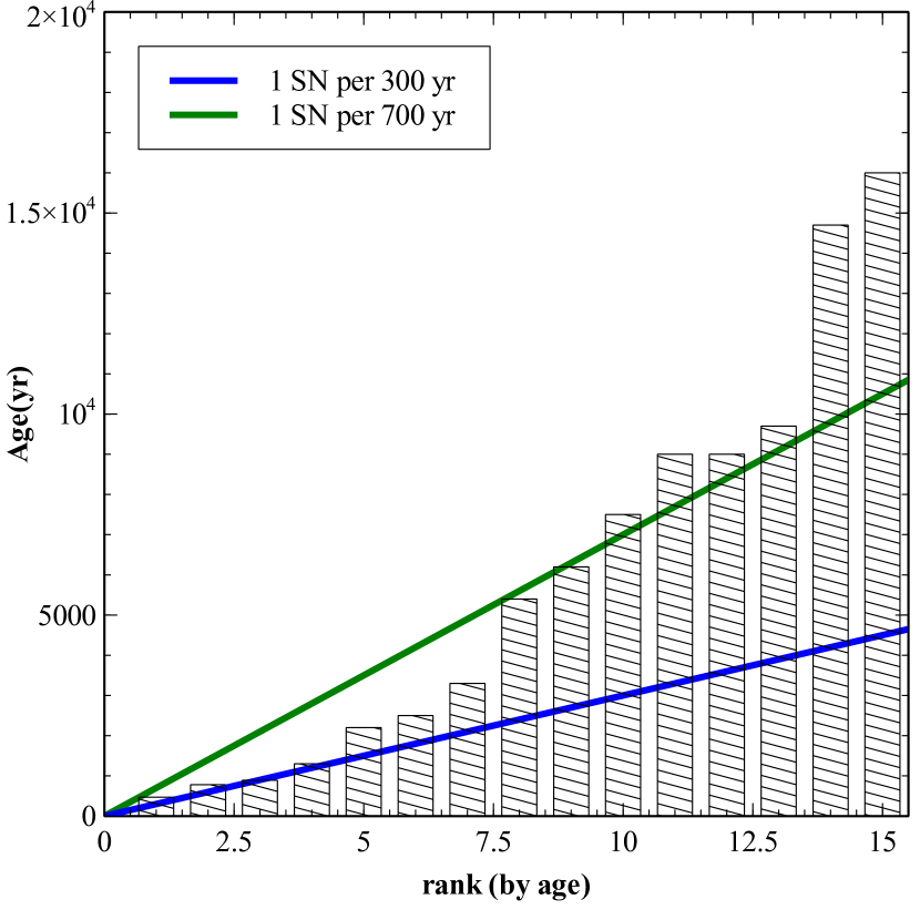
Figure 1: Cumulative distribution of model ages and fit lines for birth rate of 1 per 300 yr and 1 per 700 yr.

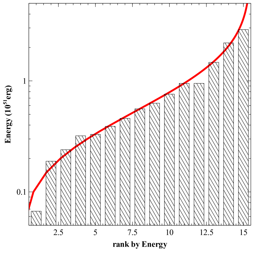
Figure 2: Cumulative distribution of model explosion energies of the 15 SNRs and fit line for a log-normal distribution of explosion energies with mean explosion energy of E₀=5.4$\times 10^{50}$ erg and variance in log(E₀) of 0.45.

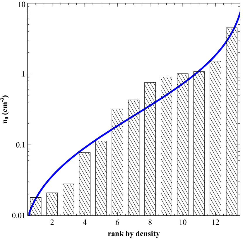
Figure 3: Cumulative distribution of model ISM densities and fit line for a log-normal distribution of ISM densities with mean density of n₀=0.26 cm^-3 and variance in log(n₀) of 0.80.

Table 1: SNR Observed Quantities

SNR	Type	Distance	Semi-axes	Radius	$EM^{a,b}$	$kT^{a,b}$	$EM_{2}^{a,b}$	$kT_{2}^{a,b}$
		(kpc)	(arcmin)	(pc)	($10^{58}$cm-3)	(keV)	($10^{58}$cm-3)	(keV)
G18.1-0.1	?	6.4$\pm$0.2	4.0$\times$3.6	7.0$\pm$0.2	8.3(2.9-21)d${}_{6.4}^{2}$	0.44(0.37-0.56)	n/a	n/a
G21.5-0.9	CC	4.4$\pm$0.2	1.8$\times$1.5	2.1$\pm$0.1	1.20(0.51-3.4)d${}_{4.4}^{2}$	0.33 (0.25-0.45)	n/a	n/a
G21.8-0.6	?	5.6$\pm$0.2	10$\times$10	16.3$\pm$0.6	0.75(0.077-0.83)d${}_{5.6}^{2}$	0.62(0.60-0.64)	n/a	n/a
G27.4+0.0	CC	5.8$\pm$0.3	2.9$\times$2.6	4.6$\pm$0.25	5.4(1.44-14.3)d${}_{5.8}^{2}$	1.60(0.90-2.4)	49(37-68)d${}_{5.8}^{2}$	0.50(0.30-0.60)
G28.6-0.1	?	9.6$\pm$0.3	12$\times$9.0	29.3$\pm$0.9	0.58(0.30-1.2)d${}_{9.6}^{2}$	0.71(0.55-0.93)	n/a	n/a
G29.7-0.3	CC	5.6$\pm$0.3	2.6$\times$1.5	3.3$\pm$0.15	0.86(0.43-1.29)d${}_{5.6}^{2}$	0.70(0.60-0.80)	n/a	n/a
G31.9+0.0	CC	7.1$\pm$0.4	4.0$\times$3.0	7.2$\pm$0.4	220(150-330)d${}_{7.1}^{2}$	0.17(0.16-0.18)	2.1(0.4-2.3)d${}_{7.1}^{2}$	0.49(0.48-0.51)
G32.8-0.1	?	4.8$\pm$0.3	12.4$\times$6.0	13.0$\pm$0.8	0.028(.014-.069)d${}_{4.8}^{2}$	0.65(0.44-0.97)	n/a	n/a
G33.6+0.1	CC	3.5$\pm$0.3	6.3$\times$5.9	6.3$\pm$0.4	2.9(2.5-4.5)d${}_{3.5}^{2}$	0.22(0.20-0.25)	0.50(.43-.57)d${}_{3.5}^{2}$	0.84(0.79-0.89)
G34.7-0.4	?	3.0$\pm$0.3	17.7$\times$12	13.0$\pm$1.3	146(132-162)d${}_{3.0}^{2}$	0.49(0.43-0.54)	n/a	n/a
G39.2-0.3	CC	8.5$\pm$0.5	3.9$\times$3.5	9.1$\pm$0.5	2.8(0.91-5.0)d${}_{8.5}^{2}$	0.68(0.49-1.05)	0.94(.74-1.14)d${}_{8.5}^{2}$	1.21(1.08-1.34)
G41.1-0.3	Ia	8.5$\pm$0.5	2.3$\times$1.3	4.45$\pm$0.25	950(650-1380)d${}_{8.5}^{2}$	0.21(0.20-0.23)	0.99(.81-1.18)d${}_{8.5}^{2}$	1.50(1.30-2.0)
G43.3-0.2	?	11.3$\pm$0.4	2.6$\times$2.6	8.55$\pm$0.3	24.6(24.4-24.8)d${}_{11.3}^{2}$	1.52(1.50-1.53)	n/a	n/a
G49.2-0.7	CC	5.6$\pm$0.6	18.5$\times$18.5	29$\pm$3.3	0.82(0.71-1.01)d${}_{5.6}^{2}$	0.70(0.65-0.76)	n/a	n/a
G54.1+0.3	CC	4.9$\pm$0.8	6.6$\times$4.5	7.9$\pm$1.3	0.26(0.125-0.39)d${}_{4.9}^{2}$	2.0(1.60-2.4)	n/a	n/a

Table 2: Basic and Electron-heating ST Model Results

	Basic ST model			ST with electron heating
SNR	Age	Energy	$n_{0}$	Age	Energy	$n_{0}$
	(yr)	($10^{51}$erg)	(cm-3)	(yr)	($10^{51}$erg)	(cm-3)
G18.1-0.1	9000	0.175	0.66	5100	0.189	0.92
G21.5-0.9	1550	0.0082	1.53	1800	0.0089	2.1
G21.8-0.6	8800	0.26	0.056	9200	0.34	0.078
G27.4+0.0	1560	0.28	0.99	1580	0.37	1.37
G28.6-0.1	14800	0.64	0.020	14200	0.96	0.028
G29.7-0.3	1690	0.030	0.65	1850	0.034	0.90
G31.9+0.0	7400	0.36	3.3	8400	0.39	4.5
G32.8-0.1	7000	0.037	0.015	5700	0.077	0.021
G33.6+0.1	5700	0.044	0.46	6500	0.048	0.64
G34.7-0.4	7900	2.1	1.09	8900	2.2	1.54
G39.2-0.3	4700	0.23	0.26	5200	0.27	0.36
G41.1-0.3	4100	0.45	13.9	4700	0.49	19.4
G43.3-0.2	2900	1.41	0.84	3200	1.70	1.17
G49.2-0.7	16700	0.89	0.020	16400	1.29	0.028
G54.1+0.3	2400	0.17	0.010	1500	0.56	0.136

Table 3: Comparison of TM Model^a and NEI Sedov model^b for LMC SNRs

SNR	Radiusc	Energyc	$n_{0}$c	Agec
	(pc)	($10^{51}$erg)	(cm-3)	($10^{3}$ yr)
J0505-6802 (N23)	6.7(H) 11.6(L)	0.46,0.53(H) 1.06(L),0.46(L2)	1.6,1.7(H) 1.5(L),3.5(L2)	3.8,3.6(H) 10.0(L),5.8(L2)
J0526-6605 (N49)	8.2(H) 10.2(L)	1.5,1.6(H) 1.2(L),0.84(L2)	2.6,2.6(H) 1.9(L),2.7(L2)	4.4,4.3(H) 7.6(L),6.2(L2)
J0535-6602 (N63A)	8.5(H) 9.80(L)	2.6,2.9(H) 2.0(L),1.6(L2)	3.9,3.9(H) 3.0(L),3.8(L2)	4.5,4.2(H) 6.6(L),5.7(L2)
J0505-6753 (DEM 71)	10.4(H) 9.4(L)	1.1,1.4(H) 0.67(L),0.77(L2)	0.67,0.86(H) 1.28(L),1.09(L2)	4.7,4.7(H) 6.8(L),7.5(L2)
J0525-6938 (N132D)	12.1(H) 13.4(L)	6.1,5.7(H) 4.8(L),4.1(L2)	2.5,2.7(H) 2.3(L),2.6(L2)	5.4,6.7(H) 8.1(L),7.3(L2)
J0453-6829 (0453-68.5)	15.0(H) 14.2(L)	0.91,1.2(H) 0.83(L),0.90(L2)	0.30,0.28(H) 0.58(L),0.53(L2)	8.7,7.4(H) 11.4(L),12.0(L2)
J0525-6559 (N49B)	17.0(H) 18.9(L)	2.7,3.1(H), 2.8(L),2.4(L2)	0.75,0.82(H) 0.51(L),0.60 (L2)	10.9,10.6(H) 11.8(L),10.7(L2)

Table 4: SNR Model Results

SNR	model typea	s	n	$M_{ej}$	Age	Energy	$n_{0}$(s=0)	$\rho_{s}$(s=2)
	(fs or rs)			($M_{\odot}$)	(yr)	($10^{51}$erg)	(cm-3)	(M⊙s/(km yr))
G18.1-0.1	fs	0	7	1.4	5400	0.189	0.92	n/a
G21.5-0.9	rs	0	9	5	470	0.56	1.01	n/a
G21.8-0.6	fs	0	7	1.4	9700	0.33	0.078	n/a
G27.4+0.0	fs	0	12	10	2500	0.32	1.08	n/a
G28.6-0.1	fs	0	7	1.4	14700	0.95	0.028	n/a
G29.7-0.3	rs	0	9	5	890	0.46	0.43	n/a
G31.9+0.0	rs	0	9	10	9000	0.39	4.5	n/a
	WL	n/a	n/a	n/a	8700	0.39	2.6	n/a
G32.8-0.1	fs	0	7	1.4	7500	0.067	0.018	n/a
G33.6+0.1	fs	2	7	20	780	2.9	n/a	6.3$\times 10^{-8}$
G34.7-0.4	fs	0	7	5	9100	2.2	1.52	n/a
	WL	n/a	n/a	n/a	9200	2.2	0.86	n/a
G39.2-0.3	fs	0	7	5	6200	0.24	0.32	n/a
G41.1-0.3	fs	2	7	1.4	1300	0.95	n/a	9.5$\times 10^{-7}$
G43.3-0.2	fs	0	7	1.4	3250	1.69	1.17	n/a
	WL	n/a	n/a	n/a	3100	1.82	0.66	n/a
G49.2-0.7	fs	0	9	10	16000	0.76	0.021	n/a
G54.1+0.3	fs	0	7	5	2200	0.63	0.113	n/a

References

- Abdo et al. (2009) Abdo, A. A., Ackermann, M., Ajello, M., et al. 2009, ApJ, 706, L1
- Anderson & Rudnick (1993) Anderson, M. C., & Rudnick, L. 1993, ApJ, 408, 514
- Auchettl et al. (2014) Auchettl, K., Slane, P., & Castro, D. 2014, ApJ, 783, 32
- Badenes et al. (2006) Badenes, C., Borkowski, K. J., Hughes, J. P., Hwang, U., & Bravo, E. 2006, ApJ, 645, 1373
- Bamba et al. (2001) Bamba, A., Ueno, M., Koyama, K., & Yamauchi, S. 2001, PASJ, 53, L21
- Bamba et al. (2016) Bamba, A., Terada, Y., Hewitt, J., et al. 2016, ApJ, 818, 63
- Becker & Helfand (1984) Becker, R. H., & Helfand, D. J. 1984, ApJ, 283, 154
- Becker & Helfand (1987) Becker, R. H., & Helfand, D. J. 1987, AJ, 94, 1629
- Bietenholz & Bartel (2008) Bietenholz, M. F., & Bartel, N. 2008, MNRAS, 386, 1411
- Bocchino et al. (2010) Bocchino, F., Bandiera, R., & Gelfand, J. 2010, A&A, 520, A71
- Borkowski et al. (2001) Borkowski, K. J., Lyerly, W. J., & Reynolds, S. P. 2001, ApJ, 548, 820
- Borkowski & Reynolds (2017) Borkowski, K. J., & Reynolds, S. P. 2017, ApJ, 846, 13
- Brogan et al. (2006) Brogan, C. L., Gelfand, J. D., Gaensler, B. M., Kassim, N. E., & Lazio, T. J. W. 2006, ApJ, 639, L25
- Camilo et al. (2002) Camilo, F., Lorimer, D. R., Bhat, N. D. R., et al. 2002, ApJ, 574, L71
- Chevalier (1982) Chevalier, R. A. 1982, ApJ, 258, 790
- Cioffi et al. (1988) Cioffi, D. F., McKee, C. F., & Bertschinger, E. 1988, ApJ, 334, 252
- Cox (1972) Cox, D. P. 1972, ApJ, 178, 159
- Cox (2005) Cox, D. P. 2005, ARA&A, 43, 337
- Ghavamian et al. (2013) Ghavamian, P., Schwartz, S. J., Mitchell, J., Masters, A., & Laming, J. M. 2013, Space Sci. Rev., 178, 633
- Green (2017) Green, D. A. 2017, VizieR Online Data Catalog, 7278,
- Grevesse & Sauval (1998) Grevesse, N., & Sauval, A. J. 1998, Space Sci. Rev., 85, 161
- Gupta et al. (2005) Gupta, Y., Mitra, D., Green, D. A., & Acharyya, A. 2005, Current Science, 89, 853
- Hanabata et al. (2013) Hanabata, Y., Sawada, M., Katagiri, H., Bamba, A., & Fukazawa, Y. 2013, PASJ, 65, 42
- Helfand et al. (1994) Helfand, D. J., Becker, R. H., Hawkins, G., & White, R. L. 1994, ApJ, 434, 627
- Hewitt et al. (2009) Hewitt, J. W., Rho, J., Andersen, M., & Reach, W. T. 2009, ApJ, 694, 1266
- Hughes et al. (1998) Hughes, J. P., Hayashi, I., & Koyama, K. 1998, ApJ, 505, 732
- Hwang et al. (2000) Hwang, U., Petre, R., & Hughes, J. P. 2000, ApJ, 532, 970
- Kawasaki et al. (2005) Kawasaki, M., Ozaki, M., Nagase, F., Inoue, H., & Petre, R. 2005, ApJ, 631, 935
- Koo et al. (2005) Koo, B.-C., Lee, J.-J., Seward, F. D., & Moon, D.-S. 2005, ApJ, 633, 946
- Kumar et al. (2014) Kumar, H. S., Safi-Harb, S., Slane, P. O., & Gotthelf, E. V. 2014, ApJ, 781, 41
- Leahy & Tian (2008) Leahy, D. A., & Tian, W. W. 2008, A&A, 480, L25
- Leahy et al. (2008) Leahy, D. A., Tian, W., & Wang, Q. D. 2008, AJ, 136, 1477
- Leahy et al. (2014) Leahy, D., Green, K., & Tian, W. 2014, MNRAS, 438, 1813
- Leahy & Ranasinghe (2016) Leahy, D. A., & Ranasinghe, S. 2016, ApJ, 817, 74
- Leahy & Williams (2017) Leahy, D. A., & Williams, J. E. 2017, AJ, 153, 239
- Leahy (2017) Leahy, D. A. 2017, ApJ, 837, 36
- Lopez et al. (2013) Lopez, L. A., Ramirez-Ruiz, E., Castro, D., & Pearson, S. 2013, ApJ, 764, 50
- Lopez et al. (2013b) Lopez, L. A., Pearson, S., Ramirez-Ruiz, E., et al. 2013, ApJ, 777, 145
- Lu et al. (2002) Lu, F. J., Wang, Q. D., Aschenbach, B., Durouchoux, P., & Song, L. M. 2002, ApJ, 568, L49
- Maggi et al. (2016) Maggi, P., Haberl, F., Kavanagh, P. J., et al. 2016, A&A, 585, A162
- Matheson & Safi-Harb (2010) Matheson, H., & Safi-Harb, S. 2010, ApJ, 724, 572
- Nadezhin (1985) Nadezhin, D. K. 1985, Ap&SS, 112, 225
- Odegard (1986) Odegard, N. 1986, AJ, 92, 1372
- Ozawa et al. (2009) Ozawa, M., Koyama, K., Yamaguchi, H., Masai, K., & Tamagawa, T. 2009, ApJ, 706, L71
- Patnaik et al. (1990) Patnaik, A. R., Hunt, G. C., Salter, C. J., Shaver, P. A., & Velusamy, T. 1990, A&A, 232, 467
- Ranasinghe & Leahy (2017) Ranasinghe, S., & Leahy, D. A. 2017, ApJ, 843, 119
- Ranasinghe & Leahy (2018a) Ranasinghe, S., & Leahy, D. A. 2018a, AJ, 155, 204
- Ranasinghe & Leahy (2018b) Ranasinghe, S., & Leahy, D. A. 2018b, MNRAS, 477, 2243
- Ranasinghe et al. (2018) Ranasinghe, S., Leahy, D. A., & Tian, W. 2018, Open Physics Journal, 4, 1
- Raymond et al. (1976) Raymond, J. C., Cox, D. P., & Smith, B. W. 1976, ApJ, 204, 290
- Reach et al. (2005) Reach, W. T., Rho, J., & Jarrett, T. H. 2005, ApJ, 618, 297
- Reynolds & Moffett (1993) Reynolds, S. P., & Moffett, D. A. 1993, AJ, 105, 2226
- Rho & Petre (1998) Rho, J., & Petre, R. 1998, ApJ, 503, L167
- Safi-Harb et al. (2005) Safi-Harb, S., Dubner, G., Petre, R., Holt, S. S., & Durouchoux, P. 2005, ApJ, 618, 321
- Sasaki et al. (2014) Sasaki, M., Heinitz, C., Warth, G., & Pühlhofer, G. 2014, A&A, 563, A9
- Sato et al. (2014) Sato, T., Koyama, K., Takahashi, T., Odaka, H., & Nakashima, S. 2014, PASJ, 66, 124
- Sato et al. (2016) Sato, T., Koyama, K., Lee, S.-H., & Takahashi, T. 2016, PASJ, 68, S8
- Seo & Hui (2013) Seo, K.-A., & Hui, C. Y. 2013, Journal of Astronomy and Space Sciences, 30, 87
- Seta et al. (2004) Seta, M., Hasegawa, T., Sakamoto, S., et al. 2004, AJ, 127, 1098
- Shimizu et al. (2012) Shimizu, T., Masai, K., & Koyama, K. 2012, PASJ, 64, 24
- Smith et al. (2011) Smith, N., Li, W., Filippenko, A. V., & Chornock, R. 2011, MNRAS, 412, 1522
- Su et al. (2009) Su, Y., Chen, Y., Yang, J., et al. 2009, ApJ, 694, 376
- Su et al. (2011) Su, Y., Chen, Y., Yang, J., et al. 2011, ApJ, 727, 43
- Tammann et al. (1994) Tammann, G. A., Loeffler, W., & Schroeder, A. 1994, ApJS, 92, 487
- Tian & Leahy (2008) Tian, W. W., & Leahy, D. A. 2008, MNRAS, 391, L54
- Tian & Leahy (2013) Tian, W. W., & Leahy, D. A. 2013, ApJ, 769, L17
- Truelove & McKee (1999) Truelove, J. K., & McKee, C. F. 1999, ApJS, 120, 299
- Uchida et al. (2012) Uchida, H., Koyama, K., Yamaguchi, H., et al. 2012, PASJ, 64, 141
- Ueno et al. (2003) Ueno, M., Bamba, A., Koyama, K., & Ebisawa, K. 2003, ApJ, 588, 338
- van den Bergh & Tammann (1991) van den Bergh, S., & Tammann, G. A. 1991, ARA&A, 29, 363
- Vasisht & Gotthelf (1997) Vasisht, G., & Gotthelf, E. V. 1997, ApJ, 486, L129
- Vink (2012) Vink, J. 2012, A&A Rev., 20, 49
- White & Long (1991) White, R. L., & Long, K. S. 1991, ApJ, 373, 543
- Wilner et al. (1998) Wilner, D. J., Reynolds, S. P., & Moffett, D. A. 1998, AJ, 115, 247
- Yamaguchi et al. (2015) Yamaguchi, H., Badenes, C., Foster, A. R., et al. 2015, ApJ, 801, L31
- Zhang et al. (2017) Zhang, M. F., Tian, W. W., Leahy, D. A., et al. 2017, ApJ, 849, 147
- Zhou et al. (2011) Zhou, X., Miceli, M., Bocchino, F., Orlando, S., & Chen, Y. 2011, MNRAS, 415, 244
- Zhou & Chen (2011) Zhou, P., & Chen, Y. 2011, ApJ, 743, 4