1 Introduction

In the last two decades, great deal of attention was devoted to miscellaneous generalizations of the Heisenberg algebra (HA) which use appropriate extensions [1, 2, 3, 4, 5, 8, 6, 7] of the relation $[X,P]={\rm i}\hbar$. Diversity of respective modifications of the famous position-momentum uncertainty relation, including those which imply minimal length, were also under study, see e.g. [3, 4, 9, 10, 11, 12] .

Recently, in ref. [8] we introduced and studied the two-parameter ($p,q$)- and three-parameter ($p,q,\mu$)-deformations of HA. In that paper (see also the two subsequent ones [13, 14]), the explicit mapping onto certain $q$- or ($p,q$)-deformed oscillator (DO) algebras was obtained. If $\mu=0$ and $p=1$, that reduces to the simplest modified HA with the $q$-commutator in the l.h.s. of its main relation and was studied earlier in [5]. Therein, the related ”target” DO algebra (DOA) was obtained as well. It is worth noting that there exists a vast number of applications of deformed oscillators or deformed bosons (to list a few [15, 16, 17, 18, 19, 20, 21, 22]).

In the cases of $q$- and ($p,q$)-deformations of HA, the formulas expressing the position and momentum operators $X,P$ in terms of the creation and destruction operators $a^{+},a^{-}$, basically differ from those (familiar linear ones) for the usual harmonic oscillator, as they involve $N$-dependent coefficients, with $N$ the excitation number operator. Caused by the required realizability of particular deformed HA through respective DOA, this fact is of great importance: it suggests real distinction from the usual Hermitian conjugation rules of the operators $a^{-}$, $a^{+}$ and others. In [13], the modified rules of (self)conjugation of the involved operators were studied in detail, with different cases listed. None of these admits Hermitian rule of conjugation of $a^{-}$ with $a^{+}$ jointly with Hermiticity of both position and momentum operators. On the other hand, it is possible that usual Hermitian conjugation rule is valid for the pair $a^{\pm}$, but $X$ and $P$ are non-hermitian.

In this paper we study the properties of some hermitian Hamiltonian built from so-called $\eta(N)$-pseudo-Hermitian position and momentum operators [8]. As note, the latter inevitably appear if one maps deformed Heisenberg algebra onto respective algebra of (nonstandard) deformed oscillator [5, 8].

Note that non-Hermitian modifications of quantum mechanics which lead nevertheless to real spectra of operators, attract great interest, see e.g. [23, 24, 25, 26, 27, 28, 29, 35, 30, 31, 33, 32]. The approach based on pseudo-Hermitian representation [27] in quantum mechanics leads to a variety of applications, ranging [33] from nonlinear optics and nuclear theory, to quantum field theory and even to biophysics.

In our approach, important role is played by the unusual $\eta(N)$-pseudo-Hermitian conjugation and the related $\eta(N)$-pseudo-Hermiticity of $X$ and/or $P$. Crucial feature is that the $\eta$-factor which performs $\eta(N)$-pseudo-Hermiticity arising within this approach due to the mentioned mapping, depends on the particle number operator $N$. That principally differs from the more common pseudo-Hermiticity (with $\eta$ depending on momentum) studied e.g. in [27, 28, 29, 33, 32]. Moreover, it was shown in [8] that in the case when $a^{+}$ and $a^{-}$ are usual Hermitian conjugates of each other, the both $X$ and $P$ should obey such $\eta(N)$-pseudo-Hermiticity. Just such situation is in the focus of this paper: i.e., we deal with the pair $a^{-}$, $a^{+}$ which are Hermitian conjugates of each other, while $X$ and $P$ are $\eta(N)$-pseudo-Hermitian (thus non-hermitian) ones, with $N$ the excitation number operator. In terms of these operators, we construct an Hermitian Hamiltonian and explore some of its properties.

The paper is organized as follows. Section 2 gives a sketch of the deformed version of HA and its mapping onto the respective DO (given by a structure function of deformation and possessing deformed analog of Fock basis), along with inclusion of the $\eta(N)$-pseudo-hermiticity aspects of operators. Then, in Sec. 3 an Hermitian Hamiltonian formed by $\eta(N)$-pseudo-Hermitian $X$ and $P$ is presented. In Sec. 4 we deal with generalized, nonlinearly extended Bogoliubov transformation (GNBT) needed to diagonalize the Hamiltonian. Section 5 is devoted to the study of unusual (given in the operator form) conditions for diagonalization. In case of so-called ”canonical” GNBT, the spectrum of the diagonalized or ”almost free” Hamiltonian is obtained in Sec. 7. The paper ends with conclusions.

2 Deformed Heisenberg algebra with $q$- or $p,q$-commutator

An approach to modify the Heisenberg algebra by deforming commutator was developed in the works [6, 5, 8, 13, 14]. Say, a one-parameter or $q$-deformed analog of HA results if one uses the $q$- commutator in the basic or defining relation:

$$XP-qPX={\rm i}\hbar\ .$$ (1)

For convenience, in all the treatment below we set $\hbar=1$.

Our main requirement, see [5, 8, 13], is that the equality (1) has to be mapped onto some DOA whose generating elements $a^{+}$, $a^{-}$ and $N$ – the creation/annihilation operators (not necessarily strict conjugates of each other) and the excitation number operator satisfy

$$[N,a^{+}]=a^{+}\ ,\hskip 22.76219pt[N,a^{-}]=-a^{-}\ ,$$ (2)

$$H(N)a^{-}a^{+}-G(N)a^{+}a^{-}=1\ \vspace{1mm}$$ (3)

where the operator functions $H(N)$ and $G(N)$ admit formal power series expansion. Note that from (2), for any function ${\cal F}(N)$ possessing formal power series expansion, we infer

$${\cal F}(N)a^{\pm}=a^{\pm}{\cal F}(N\pm 1),\hskip 19.91692pt[{\cal F}(N),a^{\pm}a^{\mp}]=0.$$ (4)

Besides (1), we will also consider the two-parameter or $p,q$-deformed analog [8] of HA whose defining relation is

$$qXP-pPX={\rm i}\hbar\,,\hskip 34.1433ptp\neq q\,,$$ (5)

where we exclude the trivial $p=q$ case as it reduces to the standard $[X,P]={\rm i}\hbar$  HA by simple rescaling of $X$ and/or $P$. Note that the deformation of HA given in ref. [11] by the relation $[X,P]={\rm i}\hbar(1+\alpha^{2}X^{2}+\beta^{2}P^{2}+\kappa XP+\kappa^{*}PX)$ can be at $\alpha=\beta=0$ related to the $q,p$-algebra (5) through juxtaposing : $\kappa=\frac{1-q}{{\rm i}\hbar}$ and $\kappa^{*}=\frac{p-1}{{\rm i}\hbar}$. That implies either $p\!=\!q\in{\bf R}$, the trivial excluded case, or the other one with $p^{*}=q=r{\rm e}^{{\rm i}\theta}$. In the latter case, one can get rid of the modulus $r$ (again by rescaling $X$ and/or $P$). For more details concerning admissible $q$, $p$ in (5) see [13].

2.1 From DHA to DOA

We are interested in its mapping onto some DOA, say, given by (2)-(3). What is important however, the desired DOA can be as well presented in a more useful form by introducing the so-called deformation structure function (DSF) $\Phi(N)$, see e.g. [36]. The latter determines the bilinears

$$a^{+}a^{-}=\Phi(N)\,,\ \ \ \ \ a^{-}a^{+}=\Phi(N+1)\,,$$ (6)

and hence the commutation relation

$$[a^{-},a^{+}]=\Phi(N+1)-\Phi(N).$$ (7)

It also determines the action formulas in the $\Phi(n)$-deformed analog of Fock space:

$$N|n\rangle=n|n\rangle,\ \ \ |n\rangle=\frac{(a^{+})^{n}}{\sqrt{\Phi(n)!}}|0\rangle,\ \ \ a^{-}|0\rangle=0$$

where $\Phi(n)!\equiv\Phi(n)\Phi(n-1)\ldots\Phi(2)\Phi(1)$ and also $\Phi(0)!=1$. In that space [36, 37],

$$\Phi(N)|n\rangle=\Phi(n)|n\rangle\,,\hskip 19.91692pta^{+}|n\rangle\!=\!\sqrt{\Phi(n\!+\!1)}|n\!+\!1\rangle,\ \ \ \ a^{-}|n\rangle\!=\!\sqrt{\Phi(n)}|n\!-\!1\rangle\ .$$ (8)

Consider first the $q$-deformed extension of HA. The desired DSF can be derived [8] if the operator functions $H(N)$, $G(N)$ are known. To find these, we set the (nonlinear) relation expressing the position/momentum operators through $a^{-}$, $a^{+}$, namely

$$X\equiv f(N)a^{-}+g(N)a^{+},\hskip 31.29802ptP\equiv{\rm i}\left(k(N)a^{+}-h(N)a^{-}\right)$$ (9)

where $f(N)$, $g(N)$, $h(N)$, $k(N)$ are some functions of the operator $N$.

After simple algebra based on (9), (5) and (3) we obtain the expressions

$$H(N)=f(N)k(N+1)+q~{}h(N)g(N+1)\ ,$$ (10)

$$G(N)=g(N)h(N-1)+q~{}k(N)f(N-1)\ .$$ (11)

For the functions $f,g,h,k$, like in [5] we have the following relations:

$$\frac{h(N\!+\!1)}{h(N)}=q\,\frac{f(N\!+\!1)}{f(N)}\,,\hskip 14.22636pt\frac{k(N\!-\!1)}{k(N)}={q}\,\frac{g(N\!-\!1)}{g(N)}\,.$$ (12)

2.2 Solutions of the relations (12) and obtaining the DSF

We need the solutions of (12) which then, using (10) and (11), yield the corresponding operator functions $G(N)$ and $H(N)$. Such solutions were found in [8, 14], and here we will deal with the following two of them.

Solution with single parameter $q$. This solution implies

$$f(N)\!=\!k(N)\!=\!\frac{1}{\sqrt{2}}\,{q}^{N},\hskip 19.91692pth(N)\!=\!g(N)\!=\!\frac{1}{\sqrt{2}}\,{q}^{2N}\ ,\vspace{-2mm}$$ (13)

from which

$$H(N)=\frac{1}{2}\,{q}^{2N+1}\Bigl{(}1+q^{2N+2}\Bigr{)}\,,\hskip 28.45274ptG(N)=\frac{1}{2}\,{q}^{2N}\Bigl{(}1+{q}^{2N-2}\Bigr{)}=\,q^{3}H(N-2).$$ (14)

Besides, putting (13) into (9), for the operators $X$ and $P$ we obtain:

$$X\!=\!\frac{1}{\sqrt{2}}\,\Bigl{(}q^{2N}a^{+}+q^{N}a^{-}\Bigr{)},\hskip 8.53581ptP\!=\!\frac{\rm i}{\sqrt{2}}\,\Bigl{(}q^{N}a^{+}\!-\!q^{2N}a^{-}\Bigr{)}.$$ (15)

Using $H(N)$ and $G(N)$ from (14), the explicit expression for the related DSF can be obtained, see [5, 8]. We will give that DSF at the end of this subsection.

Solution with two parameters $q,p$. For the $q,p$-deformed case the operators $X$ and $P$ are expressed as [14]

$$\vspace{-1mm}X=\frac{1}{\sqrt{2}}\,\Bigl{[}Q^{2N}\!a^{+}+Q^{N}\!a^{-}\Bigr{]},\hskip 19.91692ptP=\frac{\rm i}{\sqrt{2}}\,\Bigl{[}Q^{N}\!a^{+}-Q^{2N}\!a^{-}\Bigr{]},\hskip 22.76219ptQ\equiv q/p.$$ (16)

The inverse relations readily follow, namely

$$\vspace{-1mm}a^{-}\!=\!d_{N,Q}\bigl{(}Q^{-N}X\!+{\rm i}P\bigr{)},\hskip 14.22636pta^{+}\!=\!d_{N,Q}\bigl{(}X\!-{\rm i}Q^{-N}P\bigr{)},\hskip 17.07164ptd_{N,Q}\equiv\sqrt{2}(1+Q^{2N})^{-1}.$$ (17)

Obviously, at $p=1$ the latter relations give the (inverse) formulas for the $q$-deformed case. Further restriction $q=1$ implies $d_{N,1}=\frac{1}{\sqrt{2}}$ and recovers usual linear relations (see e.g. [38]) between $a^{+},a^{-}$ and $X,P$.

In the two-parameter case of $q,p$-deformed HA the operator functions $H(N)$ and $G(N)$ were also found [14] that allowed to obtain the desired DSF for (7):

$$\hskip 39.83385pt\Phi_{p,q}(n)\!=\!\frac{2p^{-1}Q^{-n}}{(1+Q^{2n-2})(1+Q^{2n})}\left(1\!+\!\frac{Q^{n}\!-\!Q^{-n+1}}{Q-1}\right)=$$

$$\ \ \ =\!\frac{2q^{-n}p^{5n-3}}{(q^{2n-2}+p^{2n-2})(q^{2n}+p^{2n})}\left(1\!+\!\frac{[2n\!-\!1]_{q,p}}{(qp)^{n-1}}\right)\,.$$ (18)

Here, $[m]_{q,p}\equiv\frac{q^{m}-p^{m}}{q-p}$ is the $q,p$-number corresponding to a number $m$, and the relation $\Phi(N)|n\rangle=\Phi(n)|n\rangle$ for the DSF, see eq. (8), has been used.

Formula (18) gives the DSF of nonstandard two-parameter deformed quantum oscillator. ”Nonstandard” means nonsymmetric under $q\leftrightarrow p$ because of the factor $q^{-n}p^{5n-3}$ in the numerator. Due to that it obviously differs from the well-known $q,p$-oscillator [34] whose structure function $\varphi_{q.p}(n)=[n]_{q,p}$ is ($q\leftrightarrow p$)-symmetric.

At last, the one-parameter or $q$-deformed DSF follows from the $p,q$-deformed one in (18) as special case if we set $p=1$. That is,

$${\Phi_{q}(n)}=\frac{2q^{-n}}{(1\!+\!q^{2n-2})(1\!+\!q^{2n})}\Bigl{(}1\!+\!\frac{q^{n}\!-\!q^{-n+1}}{q\!-\!1}\Bigr{)}=\frac{2\,q^{-n}\,[n]_{q}\,(1+q^{-n+1})}{(1+q^{2n-2})(1+q^{2n})}\,$$ (19)

where $[n]_{q}\equiv(1-q^{n})/(1-q)=\phi_{q}(n)$ (the latter coincides with the DSF of Arik-Coon deformed oscillator [39]). The obtained DSFs (16),(19) imply that now we have, besides the relation (3), also the commutation relation in the alternative form (7).

Note that from the two-parameter family with DSF in (18) one can infer, by imposing different functional relations $p\!=\!f(q)$ similarly to [40], a ”plethora” of one-parameter DOs.

3 Mutually conjugate $a^{+}$, $a^{-}$, and $\eta(N)$-pseudo-Hermitian position and momentum operators

We require that $a^{+}$ and $a^{-}$ obey the customary conjugation property:

$$(a^{\pm})^{\dagger}=a^{\mp}.$$ (20)

Then as shown in [13] it follows that both $X^{\dagger}\neq X$ and $P^{\dagger}\neq P$, and one of the possibilities is to consider these operators as $\eta(N)$-pseudo-Hermitian ones of the form

$$X^{\dagger}=\eta^{-1}_{\scriptstyle{X}}(N)\,X\,\eta_{\scriptstyle{X}}(N)\,,\hskip 28.45274ptP^{\dagger}=\eta^{-1}_{\scriptstyle{P}}(N)\,P\,\eta_{\scriptstyle{P}}(N).$$ (21)

In ref. [13], $\eta_{\scriptstyle{X}}(N)$ and $\eta^{-1}_{\scriptstyle{P}}(N)$ were found explicitly, by exploiting certain recurrence relations

$$\eta_{\scriptstyle{X}}(N+1)=\eta_{\scriptstyle{X}}(N)\,Q^{N+2}\,,\hskip 28.45274pt\eta_{\scriptstyle{P}}(N+1)=\eta_{\scriptstyle{P}}(N)\,Q^{-N+1}\,.$$

Solving of these yields

$$\eta_{\scriptstyle{X}}(N)=\ Q^{\frac{1}{2}N(N+3)}\,\eta_{\scriptstyle{X}}(0)\,,\hskip 28.45274pt\eta_{\scriptstyle{P}}(N)=\,Q^{\frac{1}{2}N(-N+3)}\,\eta_{\scriptstyle{P}}(0),$$

and the convenient choice is to set $\eta_{\scriptstyle{X}}(0)=\eta_{\scriptstyle{P}}(0)=1$. As result, we have

$$X^{\dagger}=Q^{-\frac{1}{2}N(N+3)}\,X\,Q^{\frac{1}{2}N(N+3)}\,,\hskip 28.45274ptP^{\dagger}=Q^{\frac{1}{2}N(N-3)}\,P\,Q^{-\frac{1}{2}N(N-3)}\,.$$ (22)

Although $X$ and $P$ are $\eta(N)$-pseudo-Hermitian (i.e. non-Hermitian of special form), in terms of these non-Hermitian operators we can nevertheless construct Hermitian Hamiltonian(s), see below.

Remark 1. Let us note that, as discussed in ref. [13], besides the considered case (20) of $a^{\pm}$ being mutual conjugates, there also exist the cases in which the operators $a^{+}$, $a^{-}$ are $\eta_{a}(N)$-pseudo-Hermitian conjugates of one another. For those cases, only one (or none) of the position/momentum operators can be Hermitian.

4 Hermitian Hamiltonian from non-Hermitian $X,P$

Simplest choice is to take the Hamiltonian in the familiar form $H=\frac{1}{2}\bigl{(}a^{-}a^{+}+a^{+}a^{-}\bigr{)}$ where we have set $\hbar\omega=1$. In view of (20), this form of Hamiltonian guarantees its Hermiticity. With account of the equality

$$\frac{p}{2}Q^{2N+1}\bigl{(}1+Q^{2N+2}\bigr{)}a^{-}a^{+}-\frac{p}{2}Q^{2N}\bigl{(}1+Q^{2N-2}\bigr{)}a^{+}a^{-}=1$$

which follows from (3) and the expressions (14) for $H(N)$, $G(N)$, the Hamiltonian $H$ can be presented in the form

$$H=\frac{1}{p}\ \frac{Q^{-2N-1}}{1+Q^{2N+2}}+\frac{1}{2}\biggl{(}1+Q^{-1}\frac{1+Q^{2N-2}}{1+Q^{2N+2}}\biggr{)}a^{+}a^{-}\,.$$ (23)

Besides that it is Hermitian, we can easily write down its energy spectrum $E_{n}=\frac{1}{2}\left(\Phi(n+1)+\Phi(n)\right)$, by the account of DSF $a^{+}a^{-}=\Phi(N)$ from eq. (6) applied to the Fock basis state $|n\rangle$, and taking the expression (19) for $\Phi_{q}(n)$. When $p=Q=1$, the usual harmonic oscillator with ${\cal H}={\cal H}_{0}=\frac{1}{2}+a^{+}a^{-}=N+\frac{1}{2}$ is recovered.

However, we are interested in the nontrivial Hamiltonian containing the $\eta(n)$-pseudo-Hermitian position and momentum operators considered above. It is clear that the familiar form $H=\frac{1}{2}(X^{2}+P^{2})$ is not admissible in our situation, being neither Hermitian nor pseudo-Hermitian in the deformed case (i.e. for $Q\neq 1$). That is why we suggest a natural and simple modification of $H$ which involvse the $\eta_{X}$-pseudo-Hermitian operator $X$ and $\eta_{P}$-pseudo-Hermitian operator $P$, namely

$${\cal H}=\frac{1}{2}\Bigl{(}(\eta_{X})^{-\frac{1}{2}}X^{2}(\eta_{X})^{\frac{1}{2}}+(\eta_{P})^{-\frac{1}{2}}P^{2}(\eta_{P})^{\frac{1}{2}}\Bigr{)},$$ (24)

whose Hermiticity follows from (21).

With the explicit $\eta_{X}(N)$ and $\eta_{P}(N)$ related (see [13] and Subsec. 2.3) with the case $(a^{\pm})^{\dagger}=a^{\mp}$, we have

$${\cal H}_{Q}=\frac{1}{2}\Bigl{(}Q^{-\frac{1}{4}N(N+3)}X^{2}\,Q^{\frac{1}{4}N(N+3)}+Q^{\frac{1}{4}N(N-3)}P^{2}\,Q^{-\frac{1}{4}N(N-3)}\Bigr{)}\ .$$ (25)

Using (22), we easily verify Hermiticity of ${\cal H}_{Q}$. Note that if $Q\to 1$, we recover $H=\frac{1}{2}(X^{2}+P^{2})$. Below, the Hamiltonian (25) with $Q\to q$ and the related DSF (19) will be main subject of our study.

Hermitian Hamiltonian ${\cal H}$ in (25) as nonlinear analog of Swanson model

From (15) we have

$$X^{2}=\frac{1}{2}(q^{4N-2}a^{+}a^{+}+q^{3N-1}a^{+}a^{-}+q^{3N+2}a^{-}a^{+}+q^{2N+1}a^{-}a^{-})\ ,$$

$$\hskip 19.91692ptP^{2}=-\frac{1}{2}(q^{2N-1}a^{+}a^{+}-q^{3N-2}a^{+}a^{-}-q^{3N+1}a^{-}a^{+}+q^{4N+2}a^{-}a^{-})\ .$$ (26)

Plugging these in ${\cal H}_{q}$ in eq. (25) we arrive at the (nonlinear, non-diagonal) Hermitian Hamiltonian expressed through the annihilation/creation operators, namely

$${\cal H}_{q}=A_{q}(N)a^{+}a^{+}+B_{q}(N)a^{-}a^{-}+C_{q}(N)a^{+}a^{-}+D_{q}(N)a^{-}a^{+}$$ (27)

where

$${A}_{q}(N)=\frac{1}{4}q^{3N-3}\left(q^{1/2}-q^{-1/2}\right)\ ,\hskip 34.1433pt{B}_{q}(N)=\frac{1}{4}q^{3N+3}\left(q^{1/2}-q^{-1/2}\right)\ ,$$

$$\ \ \ {C}_{q}(N)=\frac{1}{4}q^{3N-\frac{3}{2}}\left(q^{1/2}+q^{-1/2}\right)\ ,\hskip 34.1433pt{D}_{q}(N)=\frac{1}{4}q^{3N+\frac{3}{2}}\left(q^{1/2}+q^{-1/2}\right)\ .$$

The obtained Hamiltonian is reminiscent of the Swanson’s model [35] due to the presence of $a^{+}a^{+}$ and $a^{-}a^{-}$ terms. However, Swanson’s Hamiltonian is non-Hermitian because of the differing coupling constants $\alpha$, $\beta$ in front of $a^{+}a^{+}$ and $a^{-}a^{-}$ ($a^{+}$ and $a^{-}$ were taken in [35] as usual boson operators). On the other hand, in our Hamiltonian (which is Hermitian) we have, instead of numerical constants,the operator functions as ”coefficients” in front of $a^{+}a^{+}$ and $a^{-}a^{-}$. Moreover, we deal with $a^{+}$ and $a^{-}$ describing deformed bosons.

Remark 2. Notice that $A_{q}(N)\neq B_{q}(N)$ in (27). On the contrary, if we had $A_{q}(N)=B_{q}(N)$, the Hamiltonian could not be Hermitian because of relations (20) and (4). Fortunately, the explicit form of $A_{q}(N)$, $B_{q}(N)$ shows they are unequal, and related as

$${B}_{q}(N)=q^{6}{A}_{q}(N)\,,\hskip 34.1433pt{D}_{q}(N)=q^{3}\,{C}_{q}(N)\,.$$

Just this relation of proportionality of $A_{q}(N)$ and $B_{q}(N)$ provides the Hermiticity of ${\cal H}_{q}$ for real $q$, while ${C}_{q}(n)$ and ${D}_{q}(n)$ may be any real functions. In the case of phase-like $q$ i.e. $q={\rm e}^{{\rm i}\theta}$, detailed analysis shows that for such $q$ (and for general complex $q$) the Hamiltonian (27) cannot be Hermitian. So $q$ must be real, $q>0$.

Let us also note that in the no-deformation limit $q\to 1$, due to $A_{q}(N)|_{q\to 1}\to 0$ and $B_{q}(N)|_{q\to 1}\to 0$ (see (27) ), the terms containing $a^{+}a^{+}$ and $a^{-}a^{-}$ disappear from the Hamiltonian. That is, in our case the terms with $a^{+}a^{+}$ and $a^{-}a^{-}$ exist just due to deformation. In a sense, nontrivial deformation ($q\neq 1$) in our case corresponds to non-vanishing $\alpha$,  $\beta$ in Swanson’s Hamiltonian.

5 Example of $\eta(N)$-pseudo-Hermitian Hamiltonian

It is natural that in terms of $\eta_{X}(N)$-pseudo-Hermitian position and $\eta_{P}(N)$-pseudo-Hermitian momentum operators, see (21), one can easily construct an $\eta(N)$-pseudo-Hermitian Hamiltonian. Here we will present a rather simple, pseudo-Hermitian Hamiltonian which is very similar to the above Hermitian Hamiltonian.

Under the same conditions as above, i.e. for $(a^{\pm})^{\dagger}=a^{\mp}$ along with $X$, $P$ from (22) we obtain the Hamiltonian

$$\tilde{H}_{{}_{\rm PsH}}=\frac{1}{2}\left(Q^{\frac{1}{4}N(3-N)}X^{2}\,Q^{\frac{1}{4}N(N-3)}+Q^{\frac{1}{4}N(N+3)}P^{2}\,Q^{-\frac{1}{4}N(N+3)}\right).$$ (28)

One can easily verify that this is $\eta_{H}(N)$-pseudo-Hermitian with $\eta_{H}(N)=Q^{3N}$.

Remark 3. It is worth noting that the above $\eta_{H}(N)$-pseudo-hermitian Hamiltonian is very similar to the Hermitian Hamiltonian given in eq. (25). Moreover, from the $\eta_{H}(N)$-pseudo-hermitian Hamiltonian (28) one can formally obtain the Hermitian one (25) by the composition of two exchanges: $X\leftrightarrow P$ and then $q\rightarrow q^{-1}$.

Remark 4. The Hamiltonian eq. (28) can be presented in an almost ”standard” form. Indeed, denoting $\tilde{X}=Q^{-\frac{N^{2}}{4}}X\,Q^{\frac{N^{2}}{4}}$ and $\tilde{P}=Q^{\frac{N^{2}}{4}}P\,Q^{-\frac{N^{2}}{4}}$, we arrive at

$${H}_{{}_{\rm PsH}}=\frac{1}{2}Q^{\frac{3N}{4}}\bigl{(}\tilde{X}^{2}+\tilde{P}^{2}\bigr{)}Q^{-\frac{3N}{4}}\,\ \ \ \ \ {\rm or}\ \ \ \ \ \tilde{{\cal H}}=\frac{1}{2}\bigl{(}\tilde{X}^{2}+\tilde{P}^{2}\bigr{)}$$ (29)

where $\tilde{{\cal H}}\equiv Q^{-\frac{3N}{4}}H_{{}_{\rm PsH}}\,Q^{\frac{3N}{4}}$. Note also that while $X$ is $\eta_{X}(N)$-pseudo-Hermitian of the form

$$X^{\dagger}=\eta_{X}^{-1}(N)X\,\eta_{X}(N)=Q^{-\frac{1}{2}N(N+3)}X\,Q^{\frac{1}{2}N(N+3)},$$

its tilted counterpart satisfies:

$$\tilde{X}^{\dagger}=Q^{-\frac{3N}{2}}\tilde{X}\,Q^{\frac{3N}{2}}\,,$$

what means $\tilde{X}$ is $\eta_{\tilde{X}}(N)$-pseudo-Hermitian with $\eta_{\tilde{X}}(N)=Q^{\frac{3N}{2}}$.

Likewise, while $P$ is $\eta_{P}(N)$-pseudo-Hermitian of the form

$$P^{\dagger}=\eta_{P}^{-1}(N)P\,\eta_{P}(N)=Q^{\frac{1}{2}N(N-3)}P\,Q^{-\frac{1}{2}N(N-3)},$$

its tilted counterpart satisfies:

$$\tilde{P}^{\dagger}=Q^{-\frac{3N}{2}}\tilde{P}\,Q^{\frac{3N}{2}}\,,$$

what means $\tilde{P}$ is $\eta_{\tilde{P}}(N)$-pseudo-Hermitian with $\eta_{\tilde{P}}(N)=Q^{\frac{3N}{2}}$.

Hamiltonian ${H}_{\rm PsH}$ in (28) as nonlinear analog of Swanson model

Like in Hermitian case, using eq. (26) the $\eta(N)$-pseudo-Hermitian Hamiltonian (28) can also be presented in terms of annihilation/creation operators. Indeed,

$${H}_{{}_{\rm PsH}}=\tilde{A}_{N}a^{+}a^{+}+\tilde{B}_{N}a^{-}a^{-}+\tilde{C}_{N}a^{+}a^{-}+\tilde{D}_{N}a^{-}a^{+}\ ,$$ (30)

$$\ \tilde{A}_{N}=\frac{1}{4}q^{3N}\left(q^{1/2}-q^{-1/2}\right)\ ,\hskip 45.5244pt\tilde{B}_{N}=\frac{1}{4}q^{3N}\left(q^{1/2}-q^{-1/2}\right)\ ,$$

$$\ \ \ \tilde{C}_{N}=\frac{1}{4}q^{3N-\frac{3}{2}}\left(q^{1/2}+q^{-1/2}\right)\ ,\hskip 31.29802pt\tilde{D}_{N}=\frac{1}{4}q^{3N+\frac{1}{2}}\left(q^{3/2}+q^{-3/2}\right)$$

(compare with eq. (27) ). Notice that now $\tilde{A}_{N}=\tilde{B}_{N}$, $\tilde{C}_{N}=q^{-2}\tilde{D}_{N}$. Detailed study of $\eta(N)$-pseudo-Hermitian Hamiltonian (the spectrum etc.) will be done elsewhere.

6 General nonlinear Bogoliubov transformation

Basically we intend to find spectra of eigenvalues of the both Hamiltonians (27) and (30). However, since the treatment of non-Hermitian Hamiltonian is much more involved than Hermitian case, in the rest of this paper we restrict ourselves to the study of the Hermitian Hamiltonian, see Section 7 below.

In order to perform diagonalization of the Hermitian Hamiltonian (27), we have first to study general nonlinear Bogoliubov transformations (GNBT) between any two deformations of the quantum oscillator (note that some generalizations of Bogolyubov transformation involving deformed bosons were studied earlier in [41, 43, 42, 44] ). To this end, we introduce the new pair of creation/dectruction operators defined as

$$c=g_{1}{(N)}a^{+}+g_{2}{(N)}a^{-}\ ,$$ (31)

$$d=g_{3}{(N)}a^{+}+g_{4}{(N)}a^{-}\ .$$ (32)

Nonlinearity of these GNBT stems from the non-constant nature of the (operator) coefficient functions $g_{i}(N)$ of the Hermitian operator $N=\Phi^{-1}(a^{+}a^{-})$, see eq. (6).

We require $c$ and $d$ to be mutual Hermitian conjugates of one another so that

$$c^{\dagger}=d\hskip 28.45274pt\Longrightarrow\hskip 25.60747ptg_{3}{(N)}=g_{2}{(N-1)},\ \ g_{4}{(N)}=g_{1}{(N+1)}\$$

and thus

$$\ \ \ c=g_{1}{(N)}\,a^{+}+g_{2}{(N)}\,a^{-}\ ,$$ (33)

$$c^{\dagger}=g_{2}{(N\!-\!1)}\,a^{+}+g_{1}{(N\!+\!1)}\,a^{-}\ .$$ (34)

In the matrix form that reads

$$\left(\matrix{c\cr c^{\dagger}\cr}\right)=\left(\matrix{g_{2}(N)&g_{1}(N)\cr\,g_{1}(N\!+\!1)&\ \ g_{2}(N\!+\!1)\cr}\right)\!\left(\matrix{a^{-}\cr a^{+}\cr}\right)$$

where the elements of matrix are (mutually commuting) operator functions of $N$.

With the notation $c^{\dagger}\equiv c^{+}$,  $c\equiv c^{-}$, the inverse of (33), (34) is

$$a^{-}={\cal K}_{N}\left(g_{1}(N)\,c^{+}-g_{2}(N\!-\!1)\,c^{-}\right),$$ (35)

$$a^{+}={\cal K}_{N}\left(g_{1}(N\!+\!1)\,c^{-}-g_{2}(N)\,c^{+}\right)\$$ (36)

where

$${\cal K}_{N}\equiv\Bigl{(}g_{1}(N)g_{1}(N\!+\!1)-g_{2}(N)g_{2}(N\!-\!1)\Bigr{)}^{-1}.$$

Now assume that, after applying GNBT to the couple ($a^{+}$, $a^{-}$) we are led to another deformed operators $c^{+}$ and $c^{-}$ obeying the relations

$$[c^{-},c^{+}]=\chi(N+1)-\chi(N)\ ,\hskip 39.83385ptc^{+}c^{-}=\chi(N).$$ (37)

From (37) and (33)-(34), by simple algebra we infer

$$c^{-}c^{+}-c^{+}c^{-}=\left[g_{1}(N)g_{2}(N\!-\!2)-g_{2}(N\!-\!1)g_{1}(N\!-\!1)\right]a^{+}a^{+}+$$

$$+\left[g_{1}^{2}(N)-g_{2}^{2}(N\!-\!1)\right]a^{+}a^{-}+$$

$$+\left[g_{2}^{2}(N)-g_{1}^{2}(N\!+\!1)\right]a^{-}a^{+}+$$

$$\hskip 34.1433pt+\left[g_{2}(N)g_{1}(N\!+\!2)-g_{1}(N\!+\!1)g_{2}(N\!+\!1)\right]a^{-}a^{-}\ .$$

Clearly, validity of (37) imposes the following conditions

$$g_{1}(N)g_{2}(N\!-\!2)-g_{2}(N\!-\!1)g_{1}(N\!-\!1)=0,$$

$$g_{2}(N)g_{1}(N\!+\!2)-g_{1}(N\!+\!1)g_{2}(N\!+\!1)=0,$$

$$g_{1}^{2}(N)-g_{2}^{2}(N\!-\!1)=-\chi(N)/\Phi(N),\hskip 34.1433ptg_{2}^{2}(N)-g_{1}^{2}(N\!+\!1)=\chi(N+1)/\Phi(N+1)\,.$$

The first two relations are equivalent (with shift $N\to N+2$). Likewise equivalent (with shift $N\to N+1$) are the last two. Hence we have two independent relations:

$$\frac{g_{1}(N\!+\!1)}{g_{2}(N)}=\frac{g_{1}(N)}{g_{2}(N-1)}=\epsilon({\rm d.p.}),\hskip 34.1433ptg_{1}^{2}(N)-g_{2}^{2}(N\!-\!1)=-\chi(N)/\Phi(N)\,$$ (38)

where $\epsilon({\rm d.p.})\equiv\epsilon({\rm def.par.})$ reflects the fact that the ratio does not depend on $N$, but may depend on deformation parameter(s) involved in the structure functions $\chi(N)$, $\Phi(N)$. From the ratio in (38) we have $g_{2}(N\!-\!1)=\epsilon^{-1}g_{1}(N)$. Then, the explicit formulas for $g_{1}(N)$ and $g_{2}(N)$ do follow:

$$g_{1}(N)=\epsilon\,\sqrt{\frac{\chi(N)}{(1\!-\!\epsilon^{2})\,\Phi(N)}},\hskip 25.60747ptg_{2}(N)=\sqrt{\frac{\chi(N+1)}{(1\!-\!\epsilon^{2})\,\Phi(N+1)}}.$$ (39)

Let us note that if $\epsilon=\pm 1$ the formula (38) gives $\chi=0$ which in view of (37) implies $c^{+}c^{-}=c^{-}c^{+}=0$. From this and (33) we conclude that then $g_{1}=g_{2}=0$, and the whole concept of GNBT loses its sense. Hence, from now on $\epsilon\neq\pm 1$.

The obtained operator functions $g_{1}(N)$ and $g_{2}(N)$ in (39) provide most general (single-mode) nonlinear Bogoliubov transformation (33)-(34) from the deformed-boson operators $a^{+}$, $a^{-}$ (or $\Phi$-oscillator) to another deformed boson operators $c^{+}$, $c^{-}$ ($\chi$-oscillator) such that, denoting $\zeta(N)\equiv\sqrt{\Phi(N)/\chi(N)}$, we have

$$c^{-}=\frac{1}{\sqrt{1\!-\!\epsilon^{2}}}\Bigl{(}\,\epsilon\,\zeta^{-1}(N)\,a^{+}+\zeta^{-1}(N\!+\!1)\,a^{-}\Bigr{)},$$ (40)

$$c^{+}=\frac{1}{\sqrt{1\!-\!\epsilon^{2}}}\Bigl{(}\,\zeta^{-1}(N)\,a^{+}+\epsilon\,\zeta^{-1}(N\!+\!1)\,a^{-}\Bigr{)}.$$ (41)

In the matrix form this looks as

$$\left(\matrix{c^{-}\cr c^{+}\cr}\right)=||\hat{A}||\left(\matrix{a^{-}\cr a^{+}\cr}\right)\equiv\left(\matrix{\hskip 2.84526pt\frac{\zeta^{-1}(N+1)}{\sqrt{1\!-\!\epsilon^{2}}}&\ \ \ \frac{\epsilon\,\zeta^{-1}(N)}{\sqrt{1\!-\!\epsilon^{2}}}\cr\frac{\epsilon\,\zeta^{-1}(N+1)}{\sqrt{1\!-\!\epsilon^{2}}}&\ \ \frac{\zeta^{-1}(N)}{\sqrt{1\!-\!\epsilon^{2}}}\cr}\right)\!\left(\matrix{a^{-}\cr a^{+}\cr}\right),\hskip 17.07164pt\det\hat{A}=\frac{1}{\zeta(N)\,\zeta(N\!+\!1)}.$$

The operators $c^{+}$ and $c^{-}$ are mutual conjugates, and the requirement $\epsilon\neq\pm 1$ implies that $-1<\epsilon<1$. In case of $\epsilon=0$, the matrix takes diagonal form, with function of $N$ on the diagonal. This case looks similar to the familiar transformation [37] from nondeformed (or bosonic) creation/destruction operators to their deformed counterpart.

The inverse transformation reads

$$a^{-}=\frac{\zeta(N+1)}{\sqrt{1\!-\!\epsilon^{2}}}\left(c^{-}-\epsilon\,c^{+}\right),\hskip 17.07164pta^{+}=\frac{\zeta(N)}{\sqrt{1\!-\!\epsilon^{2}}}\left(c^{+}-\epsilon\,c^{-}\right),$$ (42)

or

$$\left(\matrix{a^{-}\cr a^{+}\cr}\right)=\left(\matrix{\hskip 2.84526pt\frac{\zeta(N+1)}{\sqrt{1\!-\!\epsilon^{2}}}&\ \ \ \frac{-\,\epsilon\,\zeta(N+1)}{\sqrt{1\!-\!\epsilon^{2}}}\cr\frac{-\,\epsilon\,\zeta(N)}{\sqrt{1\!-\!\epsilon^{2}}}&\ \ \frac{\zeta(N)}{\sqrt{1\!-\!\epsilon^{2}}}\cr}\right)\!\left(\matrix{c^{-}\cr c^{+}\cr}\right),\hskip 25.60747pt\det\hat{A}^{-1}=\zeta(N)\,\zeta(N+1).$$ (43)

Remark 5. The nonlinear Bogolyubov transformation that preserves commutation relation up to some constant multiplier $\kappa_{q}\equiv\kappa(q)$ so that

$$\chi(N)=\kappa_{q}\,\Phi(N)\,,\hskip 39.83385pt\lim_{q\to 1}\kappa_{q}=1\,,$$ (44)

will be called canonical GNBT. In this case we have $\zeta(N)=\kappa_{q}^{-1/2}$, i.e. zeta is a the constant. In particular, $\kappa_{q}$ may be put equal to 1 that implies $\zeta(N)=1$. Recall that usual canonical Bogolyubov transformation transforms bosons into bosons. In the canonical case, the GNBT and their inverse read:

$$c^{-}=\frac{\kappa_{q}^{1/2}}{\sqrt{1\!-\!\epsilon^{2}}}\left(\epsilon\,a^{+}+a^{-}\right),\hskip 17.07164ptc^{+}=\frac{\kappa_{q}^{1/2}}{\sqrt{1\!-\!\epsilon^{2}}}\left(a^{+}+\epsilon\,a^{-}\right),$$ (45)

$$a^{-}=\frac{\kappa_{q}^{-1/2}}{\sqrt{1\!-\!\epsilon^{2}}}\left(c^{-}-\epsilon\,c^{+}\right),\hskip 17.07164pta^{+}=\frac{\kappa_{q}^{-1/2}}{\sqrt{1\!-\!\epsilon^{2}}}\left(c^{+}-\epsilon\,c^{-}\right).$$ (46)

7 Hamiltonian for general case of quasi-particles

Now let us go back to the Hermitian Hamiltonian (27). With the account of (43), the Hamiltonian is expressed through the new deformed operators $c^{+}$ and $c^{-}$, i.e.

$${\cal H}_{q,\epsilon}=\frac{1}{1\!-\!\epsilon^{2}}R_{q}(N)\,c^{+}\,\zeta(N)\,c^{+}+\frac{\epsilon}{1\!-\!\epsilon^{2}}S_{q}(N)\,c^{+}\zeta(N+1)\,c^{+}$$

$$+\frac{\epsilon}{1\!-\!\epsilon^{2}}T_{q}(N)\,c^{-}\,\zeta(N)\,c^{-}+\frac{1}{1\!-\!\epsilon^{2}}U_{q}(N)\,c^{-}\zeta(N+1)\,c^{-}$$

$$-\frac{\epsilon}{1\!-\!\epsilon^{2}}R_{q}(N)\,c^{+}\,\zeta(N)\,c^{-}-\frac{1}{1\!-\!\epsilon^{2}}S_{q}(N)\,c^{+}\,\zeta(N+1)\,c^{-}$$

$$-\frac{1}{1\!-\!\epsilon^{2}}T_{q}(N)\,c^{-}\,\zeta(N)\,c^{+}-\frac{\epsilon}{1\!-\!\epsilon^{2}}U_{q}(N)\,c^{-}\,\zeta(N+1)\,c^{+}$$ (47)

where

$$R_{q}(N)=A_{q}(N)\,\zeta(N)-\epsilon D_{q}(N)\zeta(N+1)\ ,\hskip 14.22636ptS_{q}(N)=\epsilon B_{q}(N)\zeta(N+1)-C_{q}(N)\zeta(N)\ ,$$

$$T_{q}(N)=\epsilon A_{q}(N)\zeta(N)-D_{q}(N)\zeta(N+1)\ ,\hskip 14.22636ptU_{q}(N)=B_{q}(N)\zeta(N+1)-\epsilon\,C_{q}(N)\zeta(N)\ .$$

In the limit $q\to 1$ we have $R_{q}(N)\,\to-\frac{\epsilon}{2}\tilde{\zeta}(N+1)$,  $S_{q}(N)\to-\frac{1}{2}\tilde{\zeta}(N)$,   $T_{q}(N)\to-\frac{1}{2}\tilde{\zeta}(N+1)$ and $U_{q}(N)\,\to-\frac{\epsilon}{2}\tilde{\zeta}(N)$ with $\tilde{\zeta}(N)\equiv\left(N/\tilde{\chi}(N)\right)^{1/2}$, so that

$${\cal H}_{q,\epsilon}\buildrel q\to 1\over{\longrightarrow}{\cal H_{\epsilon}}=\frac{1}{2(1\!-\!\epsilon^{2})}\left[\left(\tilde{\zeta}(N)c^{+}\tilde{\zeta}(N+1)c^{-}+\tilde{\zeta}(N+1)c^{-}\tilde{\zeta}(N)c^{+}\right)\right.$$

$$\hskip 42.67912pt\left.+\,\epsilon^{2}\left(\tilde{\zeta}(N)c^{-}\tilde{\zeta}(N+1)c^{+}+\tilde{\zeta}(N+1)c^{+}\tilde{\zeta}(N)c^{-}\right)\right]-$$

$$\ \ \ -\,\frac{\epsilon}{2(1\!-\!\epsilon^{2})}\left[\tilde{\zeta}(N)c^{+}\tilde{\zeta}(N+1)c^{+}+\tilde{\zeta}(N+1)c^{+}\tilde{\zeta}(N)c^{+}\right.$$

$$\hskip 34.1433pt\left.+\,\tilde{\zeta}(N)c^{-}\tilde{\zeta}(N+1)c^{-}+\tilde{\zeta}(N+1)c^{-}\tilde{\zeta}(N)c^{-}\right]\,.$$

It involves the terms with $c^{\pm}\tilde{\zeta}(N)c^{\pm}$ and $c^{\pm}\tilde{\zeta}(N+1)c^{\pm}$ if $\epsilon\neq 0$. But if $\epsilon=0$, in the reduced ($q\!\to\!1$) ”quasiparticle” Hamiltonian only the first row survives. We thus have ${\cal H}_{\epsilon}|_{\epsilon=0}=\frac{1}{2}\left(\tilde{\zeta}(N)\,c^{+}\,\tilde{\zeta}(N+1)\,c^{-}+\tilde{\zeta}(N+1)\,c^{-}\,\tilde{\zeta}(N)\,c^{+}\right)$, and use (40),(41). As result, the Hamiltonian ${\cal H}_{\epsilon}|_{\epsilon=0}$ turns into $\frac{1}{2}(a^{+}a^{-}+a^{-}a^{+})$.

On the other hand, if in (47) we set $\epsilon=0$ and let $q\neq 1$, the Hamiltonian ${\cal H}_{q}$ slightly simplifies, but still contains the terms with $c^{+}...c^{+}$ and $c^{-}...c^{-}$ namely

$${\cal H}_{q,\epsilon}|_{\epsilon=0}=A_{q}(N)\zeta(N)c^{+}\zeta(N)c^{+}+B_{q}(N)\zeta(N+1)c^{-}\zeta(N+1)c^{-}$$

$$\hskip 39.83385pt+\,C_{q}(N)\zeta(N)c^{+}\zeta(N+1)c^{-}+D_{q}(N)\zeta(N+1)c^{-}\zeta(N)c^{+}.$$

In this case we have $c^{+}=\zeta^{-1}(N)a^{+}$, $c^{-}=\zeta^{-1}(N+1)a^{-}$, which correspond to the ”diagonal” DNBT, see the comment after eq. (41). Due to that, the Hamiltonian ${\cal H}_{q}|_{\epsilon=0}$ goes over into that given in (27).

Now consider the canonical case (see Remark 5). In this case

$$R^{\rm can.}_{q}(N)\!=\!\kappa_{q}^{-1/2}\bigl{(}A_{q}(N)-\epsilon\,D_{q}(N)\bigr{)},\ \ \ \ S^{\rm can.}_{q}(N)\!=\!\kappa_{q}^{-1/2}\bigl{(}\epsilon\,B_{q}(N)-C_{q}(N)\bigr{)},$$ (48)

$$T^{\rm can.}_{q}(N)\!=\!\kappa_{q}^{-1/2}\bigl{(}\epsilon\,A_{q}(N)-D_{q}(N)\bigr{)},\ \ \ \ U^{\rm can.}_{q}(N)\!=\!\kappa_{q}^{-1/2}\bigl{(}B_{q}(N)-\epsilon\,C_{q}(N)\bigr{)},$$ (49)

and the Hamiltonian (47) takes simpler form

$${\cal H}^{\rm can.}=\frac{\kappa^{-1/2}_{q}}{1-\epsilon^{2}}\biggl{\{}\left[\bigl{(}R^{\rm can.}_{q}(N)+\epsilon S^{\rm can.}_{q}(N)\bigr{)}\,c^{+}c^{+}+\bigl{(}U^{\rm can.}_{q}(N)+\epsilon T^{\rm can.}_{q}(N)\bigr{)}\,c^{-}c^{-}\right]\biggr{.}-$$

$$\biggl{.}\hskip 48.36967pt-\left[\bigl{(}S^{\rm can.}_{q}(N)+\epsilon R^{\rm can.}_{q}(N)\bigr{)}\,c^{+}c^{-}+\bigl{(}T^{\rm can.}_{q}(N)+\epsilon U^{\rm can.}_{q}(N)\bigr{)}\,c^{-}c^{+}\right]\biggr{\}}$$

(recall that GNBTs in this case look as in (45)-(46) ).

At $q\to 1$, we have $R^{\rm can.}_{q}(N),\ U^{\rm can.}_{q}(N)\to-\frac{\epsilon}{2}$,  $S^{\rm can.}_{q}(N),\ T^{\rm can.}_{q}(N)\to-\frac{1}{2}$, and then come to

$${\cal H}^{\rm can.}|_{q=1}={\cal H}^{\rm can.}=\frac{1+\epsilon^{2}}{2(1-\epsilon^{2})}\bigl{(}c^{+}c^{-}+c^{-}c^{+}\bigr{)}-\frac{\epsilon}{1-\epsilon^{2}}\bigl{(}c^{+}c^{+}+c^{-}c^{-}\bigr{)}.$$

With account of (45)-(46) we recover ${\cal H}^{\rm can.}=H=\frac{1}{2}(a^{+}a^{-}+a^{-}a^{+})$.

Now rewrite the Hamiltonian in (47) as

$${\cal H}_{q}=\frac{1}{1\!-\!\epsilon^{2}}\Bigl{(}R_{q}(N)\,c^{+}\,\zeta(N)+\epsilon S_{q}(N)\,c^{+}\zeta(N+1)\Bigr{)}\,c^{+}$$

$$\hskip 17.07164pt+\frac{\epsilon}{1\!-\!\epsilon^{2}}\Bigl{(}\epsilon T_{q}(N)\,c^{-}\,\zeta(N)+U_{q}(N)\,c^{-}\zeta(N+1)\Bigr{)}\,c^{-}$$

$$\hskip 17.07164pt-\frac{\epsilon}{1\!-\!\epsilon^{2}}\Bigl{(}\epsilon R_{q}(N)\,c^{+}\,\zeta(N)-S_{q}(N)\,c^{+}\,\zeta(N+1)\Bigr{)}\,c^{-}$$

$$\hskip 17.07164pt-\frac{1}{1\!-\!\epsilon^{2}}\Bigl{(}T_{q}(N)\,c^{-}\,\zeta(N)-\epsilon U_{q}(N)\,c^{-}\,\zeta(N+1)\Bigr{)}\,c^{+}.$$ (50)

Requiring that the first two lines of the Hamiltonian (with the terms $c^{+}\zeta(...)\,c^{+}$ and $c^{-}\zeta(...)\,c^{-}$) must vanish, we impose the following two operator relations:

$$R_{q}(N)\,c^{+}\zeta(N)\!+\epsilon\,S_{q}(N)\,c^{+}\zeta(N+1)=0\ ,$$ (51)

$$\epsilon\,T_{q}(N)\,c^{-}\zeta(N)\!+\,U_{q}(N)\,c^{-}\zeta(N+1)=0\ .$$ (52)

Remark 6. In the canonical case (see Remark 5), the Hamiltonian (50) depends on the multiplier $\kappa_{q}$. However, $\kappa_{q}$ completely cancels out from the constraints (51) and (52). Second, if we formally put $\epsilon=0$ in the constraints then these lead to the relations $R_{q}(N)=U_{q}(N)=0$ or respectively $A_{q}(N)=B_{q}(N)=0$. But the latter can hold only at $q=1$ (i.e. no deformation). So for what follows we assume $\epsilon\neq 0$.

Now let us study the implications of (51) and (52) holding simultaneously. With the use of (40), (41) we express these relations in terms of $a^{+}$ and $a^{-}$ as

$$[x(N)\,R_{q}(N)+\epsilon_{q}S_{q}(N)]a^{+}+\epsilon_{q}[R_{q}(N)+\epsilon_{q}y(N)S_{q}(N)]a^{-}=0,$$

$$[y(N)\,U_{q}(N)+\epsilon_{q}T_{q}(N)]a^{-}+\epsilon_{q}[\epsilon_{q}x(N)T_{q}(N)+U_{q}(N)]a^{+}=0,$$

where $x(N)\equiv\zeta^{-1}(N)\zeta(N\!-\!1)$ and $y(N)\equiv\zeta^{-1}(N\!+\!1)\zeta(N\!+\!2)$. Applying the formulas (8) for the operators $a^{+},a^{-}$ acting in deformed Fock basis we have

$$\sqrt{\Phi_{q}(n+1)}\,\Bigl{(}x(n+1)\,R_{q}(n+1)+\epsilon_{q}S_{q}(n+1)\Bigr{)}|n+1\rangle+$$

$$+\epsilon_{q}\sqrt{\Phi_{q}(n)}\,\Bigl{(}R_{q}(n-1)+\epsilon_{q}y(n-1)S_{q}(n-1)\Bigr{)}|n-1\rangle=0,$$

$$\sqrt{\Phi_{q}(n+1)}\,\epsilon_{q}\Bigl{(}U_{q}(n+1)+\epsilon_{q}x(n+1)\,T_{q}(n+1)\Bigr{)}|n+1\rangle+$$

$$+\sqrt{\Phi_{q}(n)}\,\Bigl{(}\epsilon_{q}T_{q}(n-1)+y(n-1)U_{q}(n-1)\Bigr{)}|n-1\rangle=0.$$

Vectors $|n-1\rangle$ and $|n+1\rangle$ are linearly independent. Since $\Phi_{q}(n)\neq 0$, and assuming $\epsilon_{q}\neq 0$ ($\epsilon_{q}=0$ dictates $c^{+}\sim a^{+}$, $c^{-}\sim a^{-}$), we infer that the equality can be valid only if the following relation does hold:

$$x(n+1)\,R_{q}(n+1)+\epsilon_{q}S_{q}(n+1)=0,\ \ \ \ \epsilon_{q}y(n-1)\,S_{q}(n-1)+R_{q}(n-1)=0.$$

These two equations yield: $x(n)=\frac{1}{y(n)}$. Taking into account that $y(n)=\frac{1}{x(n+2)}$ we arrive at the equality $x(n)=x(n+2)$ (note that the same can be drawn basing on ($\delta^{\prime}$) ). The result means the following:

$$x(n)=\cases{\rm e}^{{\rm i}\pi n}=\cos(\pi n)=\left(-1\right)^{n};\\ {\rm const}\equiv c_{q}.$$

The first option yields

$$\frac{\zeta(n)}{\zeta(n\!-\!1)}\!=\!\sqrt{\frac{\Phi_{q}(n)\,\chi_{q}(n\!-\!1)}{\Phi_{q}(n\!-\!1)\,\chi_{q}(n)}}={\rm e}^{-{\rm i}\pi n}\ \ \ \Rightarrow\ \ \ \frac{\Phi_{q}(n)}{\chi_{q}(n)}\!=\!\frac{\Phi_{q}(n\!-\!1)}{\chi_{q}(n\!-\!1)}\ \ \ \Rightarrow\ \ \ \Phi_{q}(n)\sim\chi_{q}(n).$$

The second one means that $\zeta(n)\equiv\zeta_{q}(n)$ admits the form $\zeta_{q}(n)=c_{q}^{-n}\zeta(0)$ where $\zeta(0)$ can be set as $\zeta(0)=1$, in view of footnote on page 10. Thus, $\chi_{q}(n)=c_{q}q^{n}\Phi_{q}(n)$, which at $q\!\neq\!1$, $q^{n}\!\neq\!1$ looks as a ”modification” of the canonical case (44).

The latter analysis shows we must examine more thoroughly the case and consequences of the canonical DNBT. That will be done in the next Section.

8 Diagonalized Hamiltonian for free quasi-particles

Requiring that (51) and (52) do hold, the Hamiltonian takes the form

$${\cal\tilde{H}}_{q}=\frac{1}{\epsilon^{2}\!-\!1}\Bigl{(}\epsilon\,R_{q}(N)c^{+}\zeta(N)\,c^{-}+S_{q}(N)c^{+}\zeta(N+1)\,c^{-}\Bigr{)}$$

$$+\frac{1}{\epsilon^{2}\!-\!1}\Bigl{(}T_{q}(N)c^{-}\zeta(N)\,c^{+}+\epsilon\,U_{q}(N)c^{-}\zeta(N+1)\,c^{+}\Bigr{)}\$$ (53)

and can be also given through only two operator functions say $S_{q}(N)$ and $T_{q}(N)$:

$${\cal\tilde{H}}_{q}=-\Bigl{(}S_{q}(N)\,c^{+}\,\zeta(N+1)\,c^{-}+T_{q}(N)\,c^{-}\,\zeta(N)\,c^{+}\Bigr{)}.$$ (54)

This is quasi-free (i.e. depending on the products $c^{+}...\,c^{-}$ and $c^{-}...\,c^{+}$) Hamiltonian for quasi-particles which are most general ($\chi$-)deformed bosons whose operators obey (37).

It is hardly possible to diagonalize ${\cal\tilde{H}}_{q}$ in (54) with general deformation function $\chi(N)$, and below we consider the case of canonical DNBT (see Remark 5). Note that in this canonical case $\zeta(N+1)=\zeta(N)=\kappa_{q}^{-1/2}$, and then we have

$${\cal\tilde{H}}_{q}\rightarrow{\cal\tilde{H}}^{\rm can.}_{q}=-\kappa_{q}^{-1/2}\Bigl{(}S^{c}_{q}(N)\,c^{+}\,c^{-}+T^{c}_{q}(N)\,c^{-}\,c^{+}\Bigr{)}.$$ (55)

In the limit $q\to 1$, we have $\kappa_{q}\to 1$, $S^{c}_{q}(N)\to-\frac{1}{2},\ T^{c}_{q}(N)\to-\frac{1}{2}$, and the familiar Hamiltonian ${\cal H}=\frac{1}{2}(a^{+}a^{-}+a^{-}a^{+})$ is recovered.

With account of Eq. (37) we come to the following Hermitian Hamiltonian for free quasi-particles expressed as a function of the excitation number operator:

$${\cal\tilde{H}}^{\rm can.}_{q}=\frac{-1}{\sqrt{\kappa_{q}}}\,\Bigl{(}S^{c}_{q}(N)\,\chi(N)+T^{c}_{q}(N)\,\chi(N+1)\Bigr{)}.$$ (56)

The spectrum of this Hamiltonian will be found in the next Subsection.

8.1 Eigenvalues of the quasi-particle Hamiltonian

In this section we examine the distinguished case of ”canonical” GNBT, see Remark 5, for which most advanced results can be achieved. Recall that in the case of usual (linear) Bogoliubov transformations, the term canonical refers to those transformations which preserve commutation relations. In the present deformed situation we impose slightly weaker requirement, that the DSF resulting after the ”canonical” GNBT being applied is equal to the initial DSF $\Phi(N)$ upto the multiplier $\kappa_{q}^{-1}$, depending on deformation parameter(s) and not depending on $N$, and such that $\lim_{q\to 1}\kappa_{q}=1\,$ is satisfied. In this (canonical) case eqs. (40)-(41) simplify and reduce to eqs. (45)-(46) (recall the action formulas (7)-(8) for $a^{+}$ and $a^{-}$).

From (56) we infer the result for the spectrum,

$$E_{n}\equiv\langle n|{\cal\tilde{H}}^{\rm can.}_{q}|n\rangle=-\sqrt{\kappa_{q}}\,\Bigl{(}S^{c}_{q}(n)\,\Phi_{q}(n)+T^{c}_{q}(n)\,\Phi_{q}(n+1)\Bigr{)}$$

where the relation (44) has been taken into account. Recalling the explicit form of $S^{c}_{q}(n)$ and $T^{c}_{q}(n)$ from (48) and (49) we finally obtain:

$$E_{n}=\frac{\,\ q^{3n}}{4}\Bigl{[}\Bigl{(}q^{1/2}+q^{-1/2}\Bigr{)}\left(q^{-3/2}\Phi_{q}(n)+q^{3/2}\Phi_{q}(n+1)\right)\Bigr{.}$$

$$\hskip 2.84526pt-\Bigl{.}\epsilon_{q}\Bigl{(}q^{1/2}-q^{-1/2}\Bigr{)}\Bigl{(}q^{3}\Phi_{q}(n)+q^{-3}\Phi_{q}(n+1)\Bigr{)}\Bigr{]}$$ (57)

where the expression for $\Phi_{q}(N)$ is given in (19).

This is our main result. It can also be equivalently presented as

$$E_{n}=E_{n}(q)=\frac{\,\ q^{3n}}{4}\Bigl{(}V_{q}\,\Phi_{q}(n)+W_{q}\,\Phi_{q}(n+1)\Bigr{)}$$ (58)

where

$$V_{q}=q^{-\frac{3}{2}}\Bigl{(}q^{1/2}+q^{-1/2}\Bigr{)}-\epsilon_{q}\,q^{3}\Bigl{(}q^{1/2}-q^{-1/2}\Bigr{)},$$

$$W_{q}=q^{\frac{3}{2}}\Bigl{(}q^{1/2}+q^{-1/2}\Bigr{)}-\epsilon_{q}\,q^{-3}\Bigl{(}q^{1/2}-q^{-1/2}\Bigr{)}.$$

Note that the ground state energy essentially depends on $q$:  $E_{0}=E_{0}(q)=\frac{W_{q}}{2q(1+q^{2})}$.

It only remains to examine the properties of $\epsilon_{q}$ and admissible $q$.

8.2 Function $\epsilon_{q}$ and admissible values of deformation parameter

So let us explore the explicit form and main properties of $\epsilon=\epsilon(q)\equiv\epsilon_{q}$ in the expression for energy eigenvalues $E_{n}=E_{q}(n)$. To this end we apply the relations (49)-(50). In the canonical case these take the form

$$\left(R^{c}_{q}(N)+\epsilon_{q}\,S^{c}_{q}(N)\right)\,c^{+}=0\ ,\ \ \ \ \ \left(\epsilon_{q}\,T^{c}_{q}(N)\,+\,U^{c}_{q}(N)\right)\,c^{-}=0\$$ (59)

where $R^{c}_{q}(N),\ S^{c}_{q}(N),\ T^{c}_{q}(N),\ U^{c}_{q}(N)$ are the same as in eqs. (48)-(49). For validity of these relations for all $N$, the two-term sums in each bracket should equal to zero. Having acted on Fock basis states $|n\rangle$ this gives

$$\epsilon^{2}_{q}\,A_{q}-\epsilon_{q}\,\left(C_{q}+D_{q}\right)+B_{q}=0,\ \ \ \ \ \epsilon^{2}_{q}\,B_{q}-\epsilon_{q}\,\left(C_{q}+D_{q}\right)+A_{q}=0$$

where $A_{q},\ B_{q},\ C_{q},\ D_{q}$ are given in (27), and it is meant that $q\neq 0\ {\rm nor}\ 1$ (the latter implies $\epsilon_{q}\neq 0$ ). Requiring compatibility of solutions of the two relations, we find the following possibilities:

$$A_{q}B_{q}\neq 0\ \ \ C_{q}+D_{q}\neq 0\,:\ \ \ \epsilon_{q}=\frac{A_{q}+B_{q}}{C_{q}+D_{q}}\,;$$ (60)

$$A_{q}+B_{q}\neq 0\,:\ \ \ {\tilde{\epsilon}}^{2}_{q}(A_{q}+B_{q})-2{\tilde{\epsilon}}_{q}(C_{q}+D_{q})+A_{q}+B_{q}=0.$$ (61)

Case (A).  This corresponds to eq. (60). Since both $A_{q}B_{q}\neq 0$,  $C_{q}+D_{q}\neq 0$  and $q\neq 0\ {\rm nor}\ 1$, for positive $q$ from (60) we deduce:

$$\epsilon_{q}=q^{-\frac{1}{2}}\,\frac{(q-1)(q^{2}+1)(q^{2}+q^{-2}-1)}{(q+1)^{2}(q+q^{-1}-1)}=q^{-\frac{3}{2}}\,\frac{(q-1)(q^{6}+1)}{(q+1)(q^{3}+1)}\equiv r^{-1}_{q}.$$ (62)

Admissible values of $q$ are such that $|\epsilon_{q}|<1$ and $\epsilon_{q}\neq 0$. Evaluation gives the result:  $-1<\epsilon_{q}<0$ for $q$ in the interval $1>q>0.4739142(\approx 0.4739)$, and  $0<\epsilon_{q}<1$ for $q$ in the range $1<q<2.11008657(\approx 2.11)$.

If $q\to q^{-1}$ we have $\epsilon_{q}\to\epsilon_{q^{-1}}=-\epsilon_{q}$. That gives the equality $W_{q}=V_{q^{-1}}$ for the coefficients in formula (58) for $E_{n}$. Now it can be rewritten as $E(n)=E_{q}(n)=\frac{q^{3n}}{4}\left[V_{q}\,\Phi_{q}(n)+V_{q^{-1}}\,\Phi_{q}(n+1)\right]\equiv E^{(1)}_{q}(n)+E^{(2)}_{q}(n)$. The obtained ranges of admitted values of $q$ for the intervals $-1<\epsilon_{q}<0$ and $0<\epsilon_{q}<1$ are interchangeable for the respective intervals of $\epsilon_{q^{-1}}$. This means that admissible $q$ cannot be common for $V_{q}$ and $V^{-1}_{q}$. Therefore, with possible physical application(s) in mind, we have to retain in the initial Hamiltonian (see eq. (27)) only one term – either that leading to $E^{(1)}_{q}(n)$ or leading to $E^{(2)}_{q}(n)$.

Case (B), linked with equation (61). Using the quantity $r_{q}$ from (62), we infer

$${\tilde{\epsilon}}_{q}=r_{q}\pm\sqrt{r_{q}^{2}-1}\,,\ \ \ q>0,\ \ \ q\neq 1\,.$$ (63)

Clearly, to the condition ${\tilde{\epsilon}}_{q}\neq\pm 1$ there corresponds the requirement $r_{q}\neq\pm 1$. Real solution of (63) is possible: 1) at $r_{q}>1$; 2) at $r_{q}<-1$. Moreover, if $r_{q}>1$ then $-1<{\tilde{\epsilon}}_{q}\equiv{\tilde{\epsilon}}^{-}_{q}=r_{q}-\sqrt{r_{q}^{2}-1}<1$, and if $r_{q}<-1$ then $-1<{\tilde{\epsilon}}_{q}\equiv{\tilde{\epsilon}}^{+}_{q}=r_{q}+\sqrt{r_{q}^{2}-1}<1$. Hence it remains to clarify for which values of $q>0$ the conditions 1) and 2) are valid. The analysis yields that 1) $r_{q}>1$ if $1<q<2.11008657(\approx 2.11)$, and 2) $r_{q}<-1$ when $1>q>0.4739142(\approx 0.4739)$.

If $q\to q^{-1}$ we have $r_{q}\to r_{q^{-1}}=-r_{q}$ and thus ${\tilde{\epsilon}}^{\pm}_{q}\to-{\tilde{\epsilon}}^{\mp}_{q}$ so that, unlike in previous Case A, now we have ${\tilde{\epsilon}}^{\pm}_{q^{-1}}=-\Bigl{(}r_{q}\mp\sqrt{r^{2}_{q}-1}\Bigr{)}=-{\tilde{\epsilon}}^{\mp}_{q}\neq-{\tilde{\epsilon}}^{\pm}_{q}$. Therefore in this case $W_{q}\neq V_{q^{-1}}$, and in the expression for $E_{q}(n)$ we may operate, unlike Case A,r with the both two terms, the one with $\Phi_{q}(n)$ and the othe with $\Phi_{q}(n+1)$.

Thus the obtained two expressions ${\tilde{\epsilon}}^{\pm}_{q}\neq 0$ belonging to the interval $-1<{\tilde{\epsilon}}^{\pm}_{q}<1$ and satisfying eq. (65) provide most general solution for the problem of spectrum of the deformed Hamiltonian eq. (27) (transformed into eq. (54) and then into eq. (56)). Herein, the range of admissible values of deformation parameter $q$ covers the interval $0.4739<q<2.11$ (with $q=1$ dropped).

In Figs. 1 and 2 we plot the energy spectrum function (58) at different values of deformation parameter. We observe the nontrivial (namely non-monotonic) behavior of $E_{q}(n)$ as function of $n$. Such type of behavior suggests [40] a possibility of pairwise accidental degeneracy of chosen (pairs of) energy levels at certain $q$.

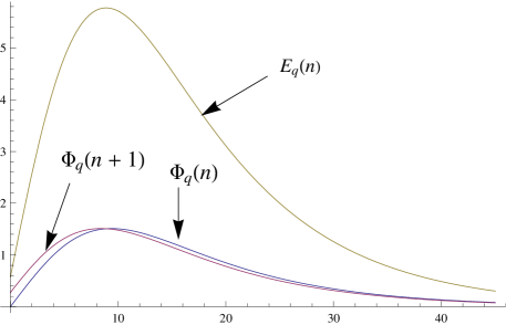
Figure 1: The functions $\Phi_{q}(n)$, $\Phi_{q}(n+1)$, and $E_{q}(n)$ versus excitation number $n$, at fixed $q=1.1$.

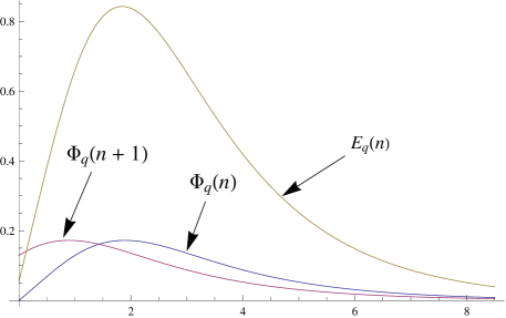
Figure 2: The functions $\Phi_{q}(n)$, $\Phi_{q}(n+1)$, and $E_{q}(n)$ versus excitation number $n$, at fixed $q=0.59$.

Concluding remarks

In this paper we have constructed the Hermitian Hamiltonian from non-Hermitian ingredients – $\eta_{X}(N)$-pseudo-Hermitian position operator $X$ and $\eta_{P}(N)$-pseudo-Hermitian momentum operator $P$, and explored its properties. Because of high (in fact non-polynomial) nonlinearity of the Hamiltonian, we have developed the generalized nonlinear Bogoliubov transformation which essentially differ from the usual ones (which are linear and involve $c$-number coefficients). In the distinguished case of canonical GNBT, by definition, the statistics determined by the structure function remains unchanged up to a multiplier $\kappa_{q}$, that is, $\Phi(N)$ $\to$ $\chi(N)=\kappa_{q}\Phi(N)$. A natural choice is to set $\kappa_{q}=1$.

When the GNBT has been applied with the goal to diagonalize the Hamiltonian, we have inferred the constraints that are basically different from the case of usual Bogoliubov transformations: indeed the constraints (51) and (52), based on GNBT and aimed as the tools for diagonalization, are the operator ones. It would be of interest to try to extract some physical consequences of these relations.

Our second main result is the energy spectrum (57) of the Hamiltonian diagonalized explicitly in the case of canonical GNBT. In this connection, we have analyzed in detail the ranges of admissible values of the deformation parameter $q$. The plots given in Fig. 1 and 2 show, for few chosen values of $q$, the nontrivial behavior of the spectrum as a function of the quantum number $n$.

References

• [1] I. Saavedra and K. Utreras, Phys. Lett. B 98, 74 (1981).
• [2] G. Brodimas, A. Jannussis and R. Mignani, J. Phys. A: Math. Gen. 25, L329 (1992).
• [3] A. Janussis, J. Phys. A 26, L233 (1993).
• [4] A. Kempf, J. Math. Phys. 35, 4483 (1994).
• [5] Chung W.S. and Klimyk A.U., J. Math. Phys. 37, 917 (1996).
• [6] J. Schwenk, J. Wess, Phys. Lett. B 291, 273 (1992).
• [7] M.S. Plyushchay, Ann. Phys. 245, 339 (1996).
• [8] A.M. Gavrilik and I.I. Kachurik, Mod. Phys. Lett. A 27, 1250114 (2012) (12pp).
• [9] L.J. Garay, Int. J. Mod. Phys. A 10, 145 (1995).
• [10] S. Hossenfelder, Class. Quant. Grav. 23, 1815 (2006).
• [11] C. Quesne, V.M. Tkachuk, SIGMA: Symmetry, Integrability and Geometry: Methods and Applications 3, 016 (2007).
• [12] T. Maslowski, A. Novicki and V.M. Tkachuk, J. Phys. A: Math. Theor. 45, 075309 (2012) (5 pp).
• [13] A.M. Gavrilik and I.I. Kachurik, Mod. Phys. Lett. A 31, 1650024 (2016) (15pp).
• [14] A.M. Gavrilik and I.I. Kachurik, SIGMA 12 (2016), 047 (12pp).
• [15] Z. Chang, Phys. Rep. 262, 137 (1995).
• [16] Y.-X. Liu et al., Phys. Rev. A 63, 023802 (2001).
• [17] L.V. Adamska, A.M. Gavrilik, J. Phys. A: Math. Gen. 37, 4787 (2004).
• [18] A.M. Gavrilik, SIGMA 2, paper 074, 12 pages (2006).
• [19] A.M. Gavrilik, I.I. Kachurik, Yu. A. Mishchenko, J. Phys. A: Math. Theor. 44, 475303 (2011).
• [20] A.M. Gavrilik, Yu. A. Mishchenko, Phys. Lett. A 376, 1596-1600 (2012).
• [21] A.M. Gavrilik, Yu. A. Mishchenko, J. Phys. A: Math. Theor. 46 (2013), 145301 (20pp).
• [22] A.M. Gavrilik, Yu.A. Mishchenko, Nucl. Phys. B 891, 466-481 (2015).
• [23] F.G. Scholtz, H.B. Geyer and F.J.W. Hahne, Ann. Phys. (N.Y.) vol.213, 74 (1992).
• [24] F. Cannata, G. Junker, and J. Trost, Phys. Lett. A 246, 219 (1998).
• [25] C. M. Bender, S. Boettcher, and P. N. Meisenger, J. Math. Phys. 40, 2201 (1999).
• [26] G. Levai and M. Znojil, J. Phys. A 33, 7165 (2000).
• [27] A. Mostafazadeh, J. Math. Phys. 43, 205 (2002).
• [28] Z. Ahmed, Phys. Lett. A 294, 287 (2002).
• [29] A. Mostafazadeh and A. Batal, J. Phys. A 37, 11645-11680 (2004).
• [30] C.M. Bender, Rep. Prog. Phys. 70, 947 (2007).
• [31] C.M Bender and H.F Jones, J. Phys. A 41, 244006 (2008).
• [32] B. Bagchi, A. Fring, Phys. Lett. A 373, 4307 (2009).
• [33] A. Mostafazadeh, Int. J. Geom. Meth. Mod. Phys., vol.7, no. 7, 1191 (2010).
• [34] A. Chakrabarti and R. Jagannathan, J. Phys. A: Math. Gen. 24, L711 (1991).
• [35] M.S. Swanson, J. Math. Phys. 45, 585 (2004).
• [36] S. Meljanac, M. Milekovic and S. Pallua, Phys. Lett. B 328, 55 (1994).
• [37] D. Bonatsos, Prog. Part. Nucl. Phys. 43, 537 (1999).
• [38] A.S. Davydov, Quantum Mechanics, Oxford: Pergamon, 1965.
• [39] M. Arik, D. D. Coon, J. Math. Phys. 17, 524 (1976).
• [40] A.M. Gavrilik, A.P. Rebesh, Mod. Phys. Lett. A 23, 921 (2008).
• [41] D. Gangopadhyay, Mod. Phys. Lett. A 6, 2909 (1991).
• [42] A. Zhedanov, Phys. Lett. A 165, 53 (1992).
• [43] J. Katriel, Phys. Lett. A 307, 1 (2003).
• [44] M.H. Naderi, R. Roknizadeh, M. Soltanolkotabi, Progr. Theor. Phys. 112, 797 (2004).