Neural Machine Translation Inspired Binary Code Similarity Comparison beyond Function Pairs

Abstract

Binary code analysis allows analyzing binary code without having access to the corresponding source code. A binary, after disassembly, is expressed in an assembly language. This inspires us to approach binary analysis by leveraging ideas and techniques from Natural Language Processing (NLP), a fruitful area focused on processing text of various natural languages. We notice that binary code analysis and NLP share many analogical topics, such as semantics extraction, classification, and code/text comparison. This work thus borrows ideas from NLP to address two important code similarity comparison problems. (I) Given a pair of basic blocks of different instruction set architectures (ISAs), determining whether their semantics is similar; and (II) given a piece of code of interest, determining if it is contained in another piece of code of a different ISA. The solutions to these two problems have many applications, such as cross-architecture vulnerability discovery and code plagiarism detection.

Despite the evident importance of Problem I, existing solutions are either inefficient or imprecise. Inspired by Neural Machine Translation (NMT), which is a new approach that tackles text across natural languages very well, we regard instructions as words and basic blocks as sentences, and propose a novel cross-(assembly)-lingual deep learning approach to solving Problem I, attaining high efficiency and precision. Many solutions have been proposed to determine whether two pieces of code, e.g., functions, are equivalent (called the equivalence problem), which is different from Problem II (called the containment problem). Resolving the cross-architecture code containment problem is a new and more challenging endeavor. Employing our technique for cross-architecture basic-block comparison, we propose the first solution to Problem II. We implement a prototype system InnerEye and perform a comprehensive evaluation. A comparison between our approach and existing approaches to Problem I shows that our system outperforms them in terms of accuracy, efficiency and scalability. The case studies applying the system demonstrate that our solution to Problem II is effective. Moreover, this research showcases how to apply ideas and techniques from NLP to large-scale binary code analysis.

I Introduction

Binary code analysis allows one to analyze binary code without access to the corresponding source code. It is widely used for vulnerability discovery, code clone detection, user-side crash analysis, etc. Today, binary code analysis has become more important than ever. Gartner forecasts that 8.4 billion IoT devices will be in use worldwide in 2017, up 31 percent from 2016, and will reach 20.4 billion by 2020 [22]. Due to code reuse and sharing, a single vulnerability at source code level may spread across hundreds or more devices that have diverse hardware architectures and software platforms [52]. However, it is difficult, often unlikely, to obtain the source code from the many IoT device companies. Thus, binary code analysis becomes the only feasible approach.

Given a code component that is known to contain some vulnerability and a large number of programs that are compiled for different ISAs, by finding programs that contain similar code components, more instances of the vulnerability can be found. Thus, cross-architecture binary code analysis draws great interests [52, 18, 19, 65].

Our insight. A binary, after disassembly, is represented in some assembly language. This inspires us to approach binary code analysis by learning from Natural Language Processing (NLP), a fruitful area focused on processing natural language corpora effectively and efficiently. Interestingly, the two seemingly remote areas—binary code analysis and NLP—actually share plenty of analogical topics, such as semantics extraction from code/text, summarization of paragraphs/functions, classification of code/articles, and code/text similarity comparison. We thus propose to adapt the ideas, methods, and techniques used in NLP to resolving binary code analysis problems. As a showcase, we use this idea to perform cross-architecture binary code similarity comparison.

Previous work [52, 18, 19, 65] essentially resolves the code equivalence problem at the function level: given a pair of functions, it is to determine whether they are equivalent. We consider a different problem: given a code component, which can be part of a function (e.g., the code in a web server that parses the URL) or a set of functions (e.g., an implementation of a crypto algorithm), to determine whether it is contained in a program. Thus, it is a code containment problem. The problem has been emphasized by previous work [27, 37, 45, 66, 60, 61, 38], but the proposed solutions can only work for code of the same ISA. Resolving the cross-architecture code containment problem is a new and important endeavor. A solution to this problem is critical for tasks such as fine-grained code plagiarism detection, thorough vulnerability search, and virus detection. For example, a code plagiarist may steal part of a function or a bunch of functions, and insert the stolen code into other code; that is, the stolen code is not necessarily a function. Code plagiarism detection based on searching for equivalent functions is too limited to handle such cases.

We define two concrete research problems: (I) given a pair of binary basic blocks of different instruction set architectures (ISAs), determining whether their semantics is similar or not; and (II) given a piece of critical code, determining whether it is contained in another piece of code of a different ISA. Problem I is a core sub-task in recent work on cross-architecture similarity comparison [52, 18, 19, 65], while Problem II is new.

Solution to Problem I. Problem I is one of the most fundamental problems for code comparison; therefore, many approaches have been proposed to resolve it, such as fuzzing [52] and representing a basic block using some features [18, 19, 65]. However, none of existing approaches are able to achieve both high efficiency and precision for this important problem. Fuzzing takes much time to try different inputs, while the feature-based representation is imprecise (A SVM classifier based on such features can only achieve AUC = 85% according to our evaluation). Given a pair of blocks of different architectures, they, after being disassembled, are two sequences of instructions in two different assembly languages. In light of this insight, we propose to learn from the ideas and techniques of Neural Machine Translation (NMT), a new machine translation framework based on neural networks proposed by NLP researchers that handles text across languages very well [29, 57]. NMT frequently uses word embedding and Long Short-Term Memory (LSTM), which are capable of learning features of words and dependencies between words in a sentence and encoding the sentence into a vector representation that captures its semantic meaning [50, 48, 64]. In addition to translating sentences, the NMT model has also been extended to measure the similarity of sentences by comparing their vector representations [48, 50].

We regard instructions as words and basic blocks as sentences, and consider that the task of detecting whether two basic blocks of different ISAs are semantically similar is analogous to that of determining whether two sentences of different human languages have similar meanings. Following this idea and learning from NMT, we propose a novel neural network-based cross-(assembly)-lingual basic-block embedding model, which converts a basic block into an embedding, i.e., a high dimensional numerical vector. The embeddings not only encode basic-block semantics, but also capture semantic relationships across architectures, such that the similarity of two basic blocks can be detected efficiently by measuring the distance between their embeddings.

Recent work [18, 19, 65] uses several manually selected features (such as the number of instructions and the number of constants) of a basic block to represent it. This inevitably causes significant information loss in terms of the contained instructions and the dependencies between these instructions. In contrast to using manually selected features, our NMT-inspired approach applies deep learning to automatically capturing such information into a vector. Specifically, we propose to employ LSTM to automatically encode a basic block into an embedding that captures the semantic information of the instruction sequence, just like LSTM is used in NMT to capture the semantic information of sentences. This way, our cross-(assembly)-lingual deep learning approach to Problem I achieves both high efficiency and precision (AUC = 98%).

Gemini [65] also applies neural networks. There are two main differences between Gemini and our work. First, as described above, Gemini uses manually selected features to represent a basic block. Second, Gemini handles the code equivalence problem rather than the code containment problem.

Solution to Problem II. A special case of Problem II, under the context of a single architecture, is well studied [31, 28, 2, 55, 54, 21, 37, 58, 56, 60, 27]. No prior solutions to Problem II under the cross-architecture context exist. To resolve it, we decompose the control flow graph (CFG) of the code of interest into multiple paths, each of which can be regarded as a sequence of basic blocks. Our idea is to leverage our solution to Problem I (for efficient and precise basic-block comparison), when applying the Longest Common Subsequence (LCS) algorithm to comparing the similarity of those paths (i.e., basic-block sequences). From there, we can calculate the similarity of two pieces of code quantitatively.

Note that we do not consider an arbitrary piece of code (unless it is a basic block) as a sentence, because it should not be simply treated as a straight-line sequence. For example, when a function is invoked, its code is not executed sequentially; instead, only a part of the code belonging to a particular path gets executed. The paths of a function can be scrambled (by compilers) without changing the semantics of the function.

We have implemented a prototype system InnerEye consisting of two sub-systems: InnerEye-BB to resolving Problem I and InnerEye-CC to resolving Problem II. We have evaluated InnerEye-BB in terms of accuracy, efficiency and scalability, and the evaluation results show that it outperforms existing approaches by large margins. Our case studies applying InnerEye-CC demonstrate that it can successfully resolve cross-architecture code similarity comparison tasks and is much more capable than recent work that is limited to comparison of function pairs. The datasets, neural network models, and evaluation results are publicly available.

We summarize our contributions as follows:

• We propose to learn from the successful NMT field to solve the cross-architecture binary code similarity comparison problem. We regard instructions as words and basic blocks as sentences. Thus, the ideas and methodologies for comparing the meanings of sentences in different natural languages can be adapted to cross-architecture code similarity comparison.

• We design a precise and efficient cross-(assembly)-lingual basic block embedding model. It utilizes word embedding and LSTM, which are frequently used in NMT, to automatically capture the semantics and dependencies of instructions. This is in contrast to prior work which largely ignores such information.

• We propose the first solution to the cross-architecture code containment problem. It has many applications, such as code plagiarism detection and virus detection.

• We implement a prototype InnerEye and evaluate its accuracy, efficiency, and scalability. We use real-world software across architectures to demonstrate the applications of InnerEye.

• This research successfully demonstrates that it is promising to approach binary analysis from the angle of language processing by adapting methodologies, ideas and techniques in NLP.

II Related Work

II-A Traditional Code Similarity Comparison

Mono-architecture solutions. Static plagiarism detection or clone detection includes string-based [2, 5, 16], token-based [31, 55, 54], tree-based [28, 32, 53], and PDG (program dependence graph)-based [20, 36, 13, 34]. Some approaches are source code based, and are less applicable in practice, especially concerning closed-source software; e.g., CCFINDER [31] finds equal suffix chains of source code tokens. TEDEM [53] introduces tree edit distances to measure code similarity at the level of basic blocks, which is costly for matching and does not handle all syntactical variation. Others compare the semantics of binary code using symbolic execution and theorem prover, such as BinHunt [21] and CoP [37], but they are computation expensive and thus not applicable for large codebases.

Second, dynamic birthmark based approaches include API birthmark [58, 56, 7] system call birthmark [60], function call birthmark [58], instruction birthmark [59, 51], and core-value birthmark [27]. Tamada et al. propose an API birthmark for Windows application [58]. Schuler et al. propose a dynamic birthmark for Java [56]. Wang et al. introduce two system call based birthmarks suitable for programs invoking sufficient system calls [60]. Jhi et al. propose a core-value based birthmark for detecting plagiarism [27]. However, as they rely on dynamic analysis, extending them to other architectures and adapting to embedded devices would be hard and tedious. Code coverage of dynamic analysis is another inherent challenge.

Cross-architecture solutions. Recently, researchers start to address the problem of cross-architecture binary code similarity detection. Multi-MH and Multi-k-MH [52] are the first two methods for comparing function code across different architectures. However, their fuzzing-based basic block similarity comparison and graph (i.e., CFG) matching-based algorithm are too expensive to handle a large number of function pairs. discovRE [18] utilizes pre-filtering to boost CFG based matching process, but it is still expensive, and the pre-filtering is unreliable, outputting too many false negatives. Both Esh [14] and its successor [15] define strands (data-flow slices of basic blocks) as the basic comparable unit. Esh uses SMT solver to verify function similarity, which makes it unscalable. As an improvement, the authors lift binaries to IR level and further create function-centric signatures [15].

II-B Machine Learning-based Code Similarity Comparison

Mono-architecture solutions. Recent research has demonstrated the usefulness of applying machine learning and deep learning techniques to code analysis [46, 39, 47, 26, 63, 25, 49, 23, 39]. White et al. further propose DeepRepair to detect the similarity between source code fragments [63]. Mou et al. introduce a tree-based convolutional neural network based on program abstract syntax trees to detect similar source code snippets [47]. Huo et al. devise NP-CNN [26] and LS-CNN [25] to identify buggy source code files. Asm2Vec [17] produces a numeric vector for each function based on the PV-DM model [33]. Similarity between two functions can be measured with the distances between the two corresponding representation vectors. $\alpha$Diff [35] characterizes a binary function using its code feature, invocation feature and module interactions feature, where the first category of feature is learned from raw bytes with a DNN. However, this work only focuses on similarity detection between cross-version binaries. Zheng et al. [11] independently propose to use word embedding to represent instructions, but their word-embedding model does not address the issue of out-of-vocabulary (OOV) instructions, while handling OOV words has been a critical step in NLP and is resolved in our system (Section IV-C); plus, their goal is to recover function signature from binaries of the same architecture, which is different from our cross-architecture code similarity comparison task. Nguyen et al. develop API2VEC for the API elements in source code to measure code similarity [49], which is not applicable if there are insufficient API calls.

Cross-architecture solutions. Genius [19] and Gemini [65] are two prior state-of-the-art works on cross-architecture bug search. They make use of conventional machine learning and deep learning, respectively, to convert CFGs of functions into vectors for similarity comparison. BinGo [8] introduces a selective inlining technique to capture the function semantics and extracts partial traces of various lengths to model functions. However, all of these approaches compare similarity between functions, and cannot handle code component similarity detection when only a part of a function or code cross function boundaries is reused in another program.

Summary. Currently, no solutions are able to meet all these requirements: (a) working on binary code, (b) analyzing code of different architectures, (c) resolving the code containment problem. This work fills the gap and proposes techniques for efficient cross-architecture binary code similarity comparison beyond function pairs. In addition, it is worth mentioning that many prior systems are built on basic block representation or comparison [21, 44, 37, 52, 19]; thus, they can benefit from our system which provides more precise basic block representation and efficient comparison.

III Overview

Given a query binary code component $\mathcal{Q}$, consisting of basic blocks whose relation can be represented in a control flow graph (CFG), we are interested in finding programs, from a large corpus of binary programs compiled for different architectures (e.g., x86 and ARM), that contain code components semantically equivalent or similar to $\mathcal{Q}$. A code component here can be part of a function or contain multiple functions.

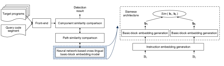
Figure 1: System architecture.

We examine code component semantics at three layers: basic blocks, CFG paths, and code components. The system architecture is shown in Figure 1. The inputs are the query code component and a set of target programs. The front-end disassembles each binary and constructs its CFG. (1) To model the semantics of a basic block, we design the neural network-based cross-lingual basic-block embedding model to represent a basic block as an embedding. The embeddings of all blocks are stored in a locality-sensitive hashing (LSH) database for efficient online search. (2) The path similarity comparison component utilizes the LCS (Longest Common Subsequence) algorithm to compare the semantic similarity of two paths, one from the query code component and another from the target program, constructed based on the LCS dynamic programming algorithm with basic blocks as the sequence elements. The length of the common subsequence is then compared to the length of the path from the query code component. The ratio indicates the semantics of the query path as embedded in the target program. (3) The component similarity comparison component explores multiple path pairs to collectively calculate a similarity score, indicating the likelihood of the query code component being reused in the target program.

Basic Block Similarity Detection. The key is to measure the similarity of two blocks, regardless of their target ISAs. As shown in the right side of Figure 1, the neural network-based cross-lingual basic-block embedding model takes a pair of blocks as inputs, and computes a similarity score $s\in[0,1]$ as the output. The objective is that the more the two blocks are similar, the closer $s$ is to $1$, and the more the two blocks are dissimilar, the closer $s$ is to $0$. To achieve this, the model adopts a Siamese architecture [6] with each side employing the LSTM [24]. The Siamese architecture is a popular network architecture among tasks that involve finding similarity between two comparable things [6, 10]. The LSTM is capable of learning long range dependencies of a sequence. The two LSTMs are trained jointly to tolerate the cross-architecture syntactic variations. The model is trained using a large dataset, which contains a large number of basic block pairs with a similarity score as the label for each pair (how to build the dataset is presented in Section V-D).

A vector representation of an instruction and a basic block is called an instruction embedding and a block embedding, respectively. The block embedding model converts each block into an embedding to facilitate comparison. Specifically, three main steps are involved in evaluating the similarity of two blocks, as shown on the right side of Figure 1. (1) Instruction embedding generation: given a block, each of its instructions is converted into an instruction embedding using an instruction embedding matrix, which is learned via a neural network (Section IV). (2) Basic-block embedding generation: the embeddings of instructions of each basic block are then fed into a neural network to generate the block embedding (Section V). (3) Once the embeddings of two blocks have been obtained, their similarity can be calculated efficiently by measuring the distance between their block embeddings.

A prominent advantage of the model inherited from Neural Machine Translation is that it does not need to select features manually when training the models; instead, as we will show later, the models automatically learn useful features during the training process. Besides, prior state-of-the-art, Genius [19] and Gemini [65], which use manually selected basic-block features, largely loses the information such as the semantics of instructions and their dependencies. As a result, the precision of our approach outperforms theirs by large margin. This is shown in our evaluation (Section VII-E3).

IV Instruction Embedding Generation

An instruction includes an opcode (specifying the operation to be performed) and zero or more operands (specifying registers, memory locations, or literal data). For example, mov eax, ebx is an instruction where mov is an opcode and both eax and ebx are operands. In NMT, words are usually converted into word embeddings to facilitate further processing. Since we regard instructions as words, similarly we represent instructions as instruction embeddings.

Our notations use blackboard bold upper case to denote functions (e.g., $\mathbb{F}$), capital letters to denote basic blocks (e.g., B), bold upper case to represent matrices (e.g., U, W), bold lower case to represent vectors (e.g., x, $\textbf{y}_{i}$), and lower case to represent individual instructions in a basic block (e.g., $x_{1}$, $y_{2}$).

IV-A Background: Word Embedding

A unique aspect of NMT is its frequent use of word embeddings, which represent words in a high-dimensional space, to facilitate the further processing in neural networks. In particular, a word embedding is to capture the contextual semantic meaning of the word; thus, words with similar contexts have embeddings close to each other in the high-dimensional space. Recently, a series of models [42, 43, 4] based on neural networks have been proposed to learn high-quality word embeddings. Among these models, Mikolov’s skip-gram model is popular due to its efficiency and low memory usage [42].

Figure 2: A sliding window used in skip-gram.

The skip-gram model learns word embeddings by using a neural network. During training, a sliding window is employed on a text stream. In Figure 2, for example, a window of size 2 is used, covering two words behind the current word and two words ahead. The model starts with a random vector for each word, and then gets trained when going over each sliding window. In each sliding window, the embedding of the current word, w_t, is used as the parameter vector of a softmax function (Equation 1) that takes an arbitrary word $w_{k}$ as a training input and is trained to predict a probability of 1, if $w_{k}$ appears in the context $C_{t}$ (i.e., the sliding window) of $w_{t}$, and 0, otherwise.

$$P(w_{k}\in C_{t}|w_{t})=\frac{\texttt{exp}(\textbf{w}_{t}^{T}\textbf{w}_{k})}{\sum_{w_{i}\in C_{t}}\texttt{exp}(\textbf{w}_{t}^{T}\textbf{w}_{i})}$$ (1)

where w_k, w_t, and w_i are the embeddings of words $w_{k}$, $w_{t}$, and $w_{i}$, respectively.

Thus, given an arbitrary word $w_{k}$, its vector representation w_k is used as a feature vector in the softmax function parameterized by w_t. When trained on a sequence of $T$ words, the model uses stochastic gradient descent to maximize the log-likelihood objective $J(\texttt{w})$ as showed in Equation 2.

$$J(w)=\frac{1}{T}\sum_{t=1}^{T}\sum_{w_{k}\in C_{t}}(\texttt{log}\hskip 2.0ptP(w_{k}|w_{t}))$$ (2)

However, it would be very expensive to maximize $J(\texttt{w})$, because the denominator $\sum_{w_{i}\in C_{t}}\texttt{exp}(\textbf{w}_{t}^{T}\textbf{w}_{i})$ sums over all words $w_{i}$ in $C_{t}$. To minimize the computational cost, popular solutions are negative sampling and hierarchical softmax. We adopt the skip-gram with negative sampling model (SGNS) [43]. After the model is trained on many sliding windows, the embeddings of each word become meaningful, yielding similar vectors for similar words. Due to its simple architecture and the use of the hierarchical softmax, the skip-gram model can be trained on a desktop machine at billions of words per hour. Plus, training the model is entirely unsupervised.

IV-B Challenges

Some unique challenges arise when learning instruction embeddings. First, in NMT, a word embedding model is usually trained once using large corpora, such as Wiki, and then reused by other researchers. However, we have to train an instruction embedding model from scratch.

Second, if a trained model is used to convert a word that has never appeared during training, the word is called an out-of-vocabulary (OOV) word and the embedding generation for such words will fail. This is a well-known problem in NLP, and it exacerbates significantly in our case, as constants, address offsets, labels, and strings are frequently used in instructions. How to deal with the OOV problem is a challenge.

IV-C Building Training Dataset

Because we regard blocks as sentences, we use instructions of each block, called a Block-level Instruction Stream (BIS) (Definition 1), to train the instruction embedding model.

Definition 1

(Block-level Instruction Stream) Given a basic block B, consisting of a list of instructions. The block-level instruction stream (BIS) of B, denoted as $\pi(\texttt{B})$, is defined as

$$\pi(\texttt{B})=(b_{1},\cdots,b_{n})$$

where $b_{i}$ is an instruction in B.

Preprocessing Training Data. To resolve the OOV problem, we propose to preprocess the instructions in the training dataset using the following rules: (1) The number constant values are replaced with 0, and the minus signs are preserved. (2) The string literals are replaced with <STR>. (3) The function names are replaced with FOO. (4) Other symbol constants are replaced with <TAG>. Take the following code snippets as an example: the left code snippet shows the original assembly code, and the right one is the preprocessed result.

MOVL %ESI, $.L.STR.31	MOVL ESI, <STR>
MOVL %EDX, $3	MOVL EDX, 0
MOVQ %RDI, %RAX	MOVQ RDI, RAX
CALLQ STRNCMP	CALLQ FOO
TESTL %EAX, %EAX	TESTL EAX, EAX
JE .LBB0_5	JE <TAG>

Note that the same preprocessing rules are applied to instructions before generating their embeddings. This way, we can significantly reduce the OOV cases. Our evaluation result (Section VII-C) shows that, after a large number of preprocessed instructions are collected to train the model, we encounter very few OOV cases in the later testing phase. This means the trained model is readily reusable for other researchers. Moreover, semantically similar instructions indeed have embeddings that are close to each other, as predicted.

IV-D Training Instruction Embedding Model

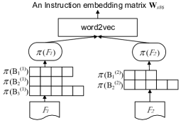
Figure 3: Learning instruction embeddings for x86. $\pi(\texttt{B}_{i}^{(j)})$ represents the $i$-th block-level instruction stream (BIS) in the function $\mathbb{F}_{j}$. Each square in a BIS represents an instruction.

We adopt the skip-gram negative sampling model as implemented in word2vec [42] to build our instruction embedding model. As an example, Figure 3 shows the process of training the model for the x86 architecture. For each architecture, an architecture-specific model is trained using the functions in our dataset containing binaries of that architecture. Each function is parsed to generate the corresponding Block-level Instruction Streams (BISs), which are fed, BIS by BIS, into the model for training. The training result is an embedding matrix containing the numerical representation of each instruction.

The resultant instruction embedding matrix is denoted by $\textbf{W}\in\mathbb{R}^{d^{e}\times V}$, where $d^{e}$ is the dimensionality of the instruction embedding selected by users (how to select $d^{e}$ is discussed in Section VII-F) and $V$ is the number of distinct instructions in the vocabulary. The i-th column of W corresponds to the instruction embedding of the i-th instruction in the vocabulary (all distinct instructions form a vocabulary).

V Block Embedding Generation

A straightforward attempt for generating the embedding of a basic block is to simply compose (e.g., summing up) all embeddings of the instruction in the basic block. However, this processing cannot handle the cross-architecture differences, as instructions that stem from the same source code but belong to different architectures may have very different embeddings. This is verified in our evaluation (Section VII-D).

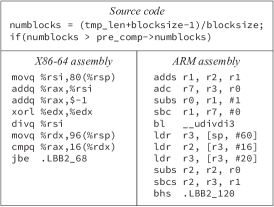
Figure 4: C source of a basic block from ec_mult.c in OpenSSL and the assembly code for two architectures.

Figure 4 shows a code snippet (containing one basic block) that has been compiled targeting two different architectures, x86-64 and ARM. While the two pieces of binary code are semantically equivalent, they look very different due to different instructions sets, CPU registers, and memory addressing modes. The basic block embedding generation should be able to handle such syntactic variation.

V-A Background: LSTM in NLP

RNN is a type of deep neural network that has been successfully applied to converting word embeddings of a sentence to a sentence embedding [12, 30]. As a special kind of RNN, LSTM is developed to address the difficulty of capturing long term memory in the basic RNN. A limit of 500 words for the sentence length is often used in practice, and a basic block usually contains less than 500 instructions.

In text analysis, LSTM treats a sentence as a sequence of words with internal structures, i.e., word dependencies. It encodes the semantic vector of a sentence incrementally, left-to-right and word-by-word. At each time step, a new word is encoded and the word dependencies embedded in the vector are “updated”. When the process reaches the end of the sentence, the semantic vector has embedded all the words and their dependencies, and hence, can be viewed as a feature representation of the whole sentence. That semantic vector is the sentence embedding.

V-B Cross-lingual Basic-block Embedding Model Architecture

Figure 5: Neural network-based basic-block embedding model. Each shaded box is an LSTM cell.

Inspired by the NMT model that compares the similarity of sentences of different languages, we design a neural network-based cross-lingual basic-block embedding model to compare the semantics similarity of basic blocks of different ISAs. As showed in Figure 5, we design our model as a Siamese architecture [6] with each side employing the identical LSTM. Our objective is to make the embeddings for blocks of similar semantics as close as possible, and meanwhile, to make blocks of different semantics as far apart as possible. A Siamese architecture takes the embeddings of instructions in two blocks, $\texttt{B}_{1}$ and $\texttt{B}_{2}$, as inputs, and produces the similarity score as an output. This model is trained with only supervision on a basic-block pair as input and the ground truth $\chi(\texttt{B}_{1},\texttt{B}_{2})$ as an output without relying on any manually selected features.

For embedding generation, each LSTM cell sequentially takes an input (for the first layer the input is an instruction embedding) at each time step, accumulating and passing increasingly richer information. When the last instruction embedding is reached, the last LSTM cell at the last layer provides a semantic representation of the basic block, i.e., a block embedding. Finally, the similarity of the two basic blocks is measured as the distance of the two block embeddings.

Detailed Process. The inputs are two blocks, $\texttt{B}_{1}$ and $\texttt{B}_{2}$, represented as a sequence of instruction embeddings, ($\textbf{e}_{1}^{(1)},\cdots,\textbf{e}_{T}^{(1)}$), and ($\textbf{e}_{1}^{(2)},\cdots,\textbf{e}_{S}^{(2)}$), respectively. Note that the sequences may be of different lengths, i.e., $|T|\neq|S|$, and the sequence lengths can vary from example to example; both are handled by the model. An LSTM cell analyzes an input vector coming from either the input embeddings or the precedent step and updates its hidden state at each time step. Each cell contains four components (which are real-valued vectors): a memory state $c$, an output gate $o$ determining how the memory state affects other units, and an input gate $i$ (and a forget gate $f$, resp.) that controls what gets stored in (and omitted from, resp.) memory. For example, an LSTM cell at the first layer in LSTM₁ updates its hidden state at the time step $t$ via Equations 3–8:

$$\footnotesize\textbf{i}_{t}^{(1)}=\texttt{sigmoid}(\textbf{W}_{i}\textbf{e}_{t}^{(1)}+\textbf{U}_{i}\textbf{x}_{t-1}^{(1)}+\textbf{v}_{i})$$ (3)

$$\footnotesize\textbf{f}_{t}^{(1)}=\texttt{sigmoid}(\textbf{W}_{f}\textbf{e}_{t}^{(1)}+\textbf{U}_{f}\textbf{x}_{t-1}^{(1)}+\textbf{v}_{f})$$ (4)

$$\footnotesize\widetilde{\textbf{c}_{t}}^{(1)}=\texttt{tanh}(\textbf{W}_{c}\textbf{e}_{t}^{(1)}+\textbf{U}_{c}\textbf{x}_{t-1}^{(1)}+\textbf{v}_{c})$$ (5)

$$\footnotesize\textbf{c}_{t}^{(1)}=\textbf{i}_{t}^{(1)}{\color[rgb]{0,0,0}\odot}\widetilde{\textbf{c}_{t}}^{(1)}+\textbf{f}_{t}^{(1)}{\color[rgb]{0,0,0}\odot}\widetilde{\textbf{c}_{t}}^{(1)}$$ (6)

$$\footnotesize\textbf{o}_{t}^{(1)}=\texttt{sigmoid}(\textbf{W}_{o}\textbf{e}_{t}^{(1)}+\textbf{U}_{o}\textbf{x}_{t-1}^{(1)}+\textbf{v}_{o})$$ (7)

$$\footnotesize\textbf{x}_{t}^{(1)}=\textbf{o}_{t}^{(1)}{\color[rgb]{0,0,0}\odot}\texttt{tanh}(\textbf{c}_{t}^{(1)})$$ (8)

where $\odot$ denotes Hadamard (element-wise) product; $\textbf{W}_{i}$, $\textbf{W}_{f}$, $\textbf{W}_{c}$, $\textbf{W}_{o}$, $\textbf{U}_{i}$, $\textbf{U}_{f}$, $\textbf{U}_{c}$, $\textbf{U}_{o}$ are weight matrices; and $\textbf{v}_{i}$, $\textbf{v}_{f}$, $\textbf{v}_{c}$, $\textbf{v}_{o}$ are bias vectors; they are learned during training. The reader is referred to [24] for more details.

At the last time step $T$, the last hidden state at the last layer provides a vector $\textbf{h}_{T}^{(1)}$ (resp. $\textbf{h}_{S}^{(2)}$ ), which is the embedding of $\texttt{B}_{1}$ (resp. $\texttt{B}_{2}$). We use the Manhattan distance ($\in[0,1]$) which is suggested by [48] to measure the similarity of $\texttt{B}_{1}$ and $\texttt{B}_{2}$ as showed in Equation 9:

$$\texttt{Sim}(\texttt{B}_{1},\texttt{B}_{2})=\texttt{exp}(-\mathbin{\|}\textbf{h}_{T}^{(1)}-\textbf{h}_{S}^{(2)}\mathbin{\|}_{1})\vspace*{-6pt}$$ (9)

To train the network parameters, we use stochastic gradient descent (SGD) to minimize the loss function:

$$\min_{\textbf{W}_{i},\textbf{W}_{f},...,\textbf{v}_{o}}\sum_{i=1}^{N}(y_{i}-\texttt{Sim}(\texttt{B}_{1}^{i},\texttt{B}_{2}^{i}))^{2}$$ (10)

where $y_{i}$ is the similarity ground truth of the pair $<\texttt{B}_{1}^{i},\texttt{B}_{2}^{i}>$, and $N$ the number of basic block pairs in the training dataset.

In the end, once the Area Under the Curve (AUC) value converges, the training process terminates, and the trained cross-lingual basic-block embedding model is capable of encoding an input binary block to an embedding capturing the semantics information of the block that is suitable for similarity detection.

V-C Challenges

There are two main challenges for learning block embeddings. First, in order to train, validate and test the basic-block embedding model, a large dataset containing labeled similar and dissimilar block pairs is needed. Unlike prior work [65] that builds the dataset of similar and dissimilar function pairs by using the function names to establish the ground truth about the function similarity, it is very challenging to establish the ground truth for basic blocks because: (a) no name is available to indicate whether two basic blocks are similar or not, and (b) even if two basic blocks have been compiled from two pieces of code, they may happen to be equivalent or similar, and therefore, it would be incorrect to label them as dissimilar.

Second, many hyperparameters need to be determined to maximize the model performance. The parameter values selected for NMT are not necessarily applicable to our model, and need to be comprehensively examined (Section VII-F).

V-D Building Dataset

V-D1 Generating Similar Basic-Block Pairs

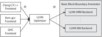
Figure 6: LLVM architecture. The basic-block boundary annotator is added into the backends of different architectures.

We consider two basic blocks of different ISAs that have been compiled from the same piece of source code as equivalent. To establish the ground truth about the block similarity, we modify the backends of various architectures in the LLVM compiler. As shown in Figure 6, the LLVM compiler consists of various frontends (that compile source code into a uniform Intermediate Representation (IR)), the middle-end optimizer, and various architecture-dependent backends (that generate the corresponding assembly code). We modify the backends to add the basic-block boundary annotator, which not only clearly marks the boundaries of blocks, but also annotates a unique ID for each generated assembly block in a way that all assembly blocks compiled from the same IR block (i.e., the same piece of source code), regardless of their architectures, will obtain the same ID.

To this end, we collect various open-sourced software projects, and feed the source code into the modified LLVM compiler to generate a large number of basic blocks for different architectures. After preprocessing (Section IV-C) and data deduplication, for each basic block B^x86, the basic block B^ARM with the same ID is sampled to construct one training example <B^x86, B^ARM, 1>. By continually sampling, we can collect a large number of similar basic-block pairs.

V-D2 Generating Dissimilar Basic-Block Pairs

While two basic blocks with the same ID are always semantically equivalent, two blocks with different IDs may not necessarily be dissimilar, as they may happen to be be equivalent.

To address this issue, we make use of $n$-gram to measure the text similarity between two basic blocks compiled for the same architecture at the same optimization level. A low text similarity score indicates two basic blocks are dissimilar. Next, assume a block B${}_{1}^{ARM}$ of ARM is equivalent to a block B${}_{1}^{x86}$ of x86 (they have the same ID); and another block B${}_{2}^{x86}$ of x86 is dissimilar to B${}_{1}^{x86}$ according to the $n$-gram similarity comparison. Then, the two blocks, B${}_{1}^{ARM}$ and B${}_{2}^{x86}$, are regarded as dissimilar, and the instance <B${}_{1}^{ARM}$, B${}_{2}^{x86}$, 0> is added to the dataset. Our experiments set $n$ as 4 and the similarity threshold as 0.5; that is, if two blocks, through this procedure, have a similarity score smaller than 0.5, they are labeled as dissimilar. This way, we can obtain a large number of dissimilar basic-block pairs across architectures.

VI Path/Code Component Similarity Comparison

Detecting similar code components is an important problem. Existing work either can only work on a single architecture [60, 21, 37, 44, 58, 56, 27], or can compare a pair of functions across architectures [52, 18, 19, 65]. However, as a critical code part may be inserted inside a function to avoid detection [28, 27, 37], how to resolve the cross-archite code containment problem is a new and more challenging problem.

We propose to decompose the CFG of the query code component $\mathcal{Q}$ into multiple paths. For each path from $\mathcal{Q}$, we compare it to many paths from the target program $\mathcal{T}$, to calculate a path similarity score by adopting the Longest Common Subsequence (LCS) dynamic programming algorithm with basic blocks as sequence elements. By trying more than one path, we can use the path similarity scores collectively to detect whether a component in $\mathcal{T}$ is similar to $\mathcal{Q}$.

VI-A Path Similarity Comparison

A linearly independent path is a path that introduces at least one new node (i.e., basic block) that is not included in any previous linearly independent paths [62]. Once the starting block of $\mathcal{Q}$ and several candidate starting blocks of $\mathcal{T}$ are identified (presented in Section VI-B), the next step is to explore paths to calculate a path similarity score. For $\mathcal{Q}$, we select a set of linearly independent paths from the starting block. We first unroll each loop in $\mathcal{Q}$ once, and adopt the Depth First Search algorithm to find a set of linearly independent paths.

For each linearly independent path of $\mathcal{Q}$, we need to find the highest similarity score between the query path and the many paths of $\mathcal{T}$. To this end, we apply a recently proposed code similarity comparison approach, called CoP [37] (it is powerful for handling many types of obfuscations but can only handle code components of the same architecture). CoP combines the LCS algorithm and basic-block similarity comparison to compute the LCS of semantically equivalent basic blocks (SEBB). However, CoP’s basic-block similarity comparison relies on symbolic execution and theorem proving, which is very computationally expensive [40]. On the contrary, our work adopts techniques in NMT to significantly speed up basic-block similarity comparison, and hence is much more scalable for analyzing large codebases.

Here we briefly introduce how CoP applies LCS to detect path similarity. It adopts breadth-first search in the inter-procedural CFG of the target program $\mathcal{T}$, combined with the LCS dynamic programming to compute the highest score of the LCS of SEBB. For each step in the breadth-first dynamic programming algorithm, the LCS is kept as the “longest path” computed so far for a block in the query path. The LCS score of the last block in the query path is the highest LCS score, and is used to compute a path similarity score. Definition 2 gives a high-level description of a path similarity score.

Definition 2

(Path Similarity Score) Given a linearly independent path $\mathcal{P}$ from the query code component, and a target program $\mathcal{T}$. Let $\Gamma=\{\mathcal{P}_{1}^{t},\ldots,\mathcal{P}_{n}^{t}\}$ be all of the linearly independent paths of $\mathcal{T}$, and $|\mathrm{LCS}(\mathcal{P},\mathcal{P}_{i}^{t})|$ be the length of the LCS of SEBB between $\mathcal{P}$ and $\mathcal{P}_{i}^{t}$, $\mathcal{P}_{i}^{t}\in\Gamma$. Then, the path similarity score for $\mathcal{P}$ is defined as

$$\psi(\mathcal{P},T)=\frac{\max\nolimits_{\mathcal{P}_{i}^{t}\in\Gamma}|\mathrm{LCS}(\mathcal{P},\mathcal{P}_{i}^{t})|}{|\mathcal{P}|}$$

VI-B Component Similarity Comparison

Challenge. The location that the code component gets embedded into the containing target program is unknown, and it is possible for it to be inserted into the middle of a function. It is important to determine the correct starting points so that the path exploration is not misled to irrelevant code parts of the target program. This is a unique challenge compared to function-level code similarity comparison.

Idea. We look for the starting blocks in the manner as follows. First, the embeddings of all basic blocks of the target program $\mathcal{T}$ are stored in an locality-sensitive hashing database for efficient online search. Next, we begin with the first basic block in the query code component $\mathcal{Q}$ as the starting block, and search in the database to find a semantically equivalent basic block (SEBB) from the target program $\mathcal{T}$. If we find one or several SEBBs, we proceed with the path exploration (Section VI-A) on each of them. Otherwise, we choose another block from $\mathcal{Q}$ as the starting block [37], and repeat the process until the last block of $\mathcal{Q}$ is checked.

Component similarity score. We select a set of linearly independent paths from $\mathcal{Q}$, and compute a path similarity score for each linearly independent path. Next, we assign a weight to each path similarity score according to the length of the corresponding query path. The final component similarity score is the weighted average score.

Summary. By integrating our cross-lingual basic-block embedding model with an existing approach [37], we have come up with an effective and efficient solution to cross-architecture code-component similarity comparison. Moreover, it demonstrates how the efficient, precise and scalable basic-block embedding model can benefit many other systems [21, 37, 44] that rely on basic-block similarity comparison.

VII Evaluation

We evaluate InnerEye in terms of its accuracy, efficiency, and scalability. First, we describe the experimental settings (Section VII-A) and discuss the datasets used in our evaluation (Section VII-B). Next, we examine the impact of preprocessing on out-of-vocabulary instructions (Section VII-C) and the quality of the instruction embedding model (Section VII-D). We then evaluate whether InnerEye-BB can successfully detect the similarity of blocks compiled for different architectures (Problem I). We evaluate its accuracy and efficiency (Sections VII-E and VII-G), and discuss hyperparameter selection (Section VII-F). We also compare it with a machine learning-based basic-block comparison approach that uses a set of manually selected features [19, 65] (Section VII-E3). Finally, we present three real-world case studies demonstrating how InnerEye-CC can be applied for cross-architecture code component search and cryptographic function search under realistic conditions (Problem II) in Section VII-H.

VII-A Experimental Settings

We adopt word2vec [42] to learn instruction embeddings, and implemented our cross-lingual basic-block embedding model in Python using the Keras [9] platform with TensorFlow [1] as backend. Keras provides a large number of high-level neural network APIs and can run on top of TensorFlow. Like the work CoP [37], we require that the selected linearly independent paths cover at least 80% of the basic blocks in each query code component; the largest number of the selected linearly independent paths in our evaluation is 47. InnerEye-CC (the LCS algorithm with path exploration) is implemented in the BAP framework [3] which constructs CFGs and call graph and builds the inter-procedural CFG. InnerEye-CC queries the block embeddings (computed by InnerEye-BB) stored in an LSH database. The experiments are performed on a computer running the Ubuntu 14.04 operating system with a 64-bit 2.7 GHz Intel^® Core^(TM) i7 CPU and 32 GB RAM without GPUs. The training and testing are expected to be significantly accelerated if GPUs are used.

VII-B Dataset

TABLE I: The number of basic-block pairs in the training, validation and testing datasets.

	Training			Validation			Testing			Total
	Sim.	Dissim.	Total	Sim.	Dissim.	Total	Sim.	Dissim.	Total	Sim.	Dissim.	Total
O1	35,416	35,223	70,639	3,902	3,946	7,848	4,368	4,354	8,722	43,686	43,523	87,209
O2	45,461	45,278	90,739	5,013	5,069	10,082	5,608	5,590	11,198	56,082	55,937	112,019
O3	48,613	48,472	97,085	5,390	5,397	10,787	6,000	5,988	11,988	60,003	59,857	119,860
Cross-opts	34,118	33,920	68,038	3,809	3,750	7,559	4,554	4,404	8,958	42,481	42,074	84,555
Total	163,608	162,893	326,501	18,114	18,162	36,276	20,530	20336	40,866	202,252	201,391	403,643

We first describe the dataset (Dataset I), as shown in Table I, used to evaluate the cross-lingual basic-block embedding model (InnerEye-BB). All basic-block pairs in the dataset are labeled with the similarity ground truth. In particular, we prepare this dataset using OpenSSL (v1.1.1-pre1) and four popular Linux packages, including coreutils (v8.29), findutils (v4.6.0), diffutils (v3.6), and binutils (v2.30). We use two architectures (x86-64 and ARM) and clang (v6.0.0) with three different optimization levels (O1-O3) to compile each program. In total, we obtain 437,104 basic blocks for x86, and 393,529 basic blocks for ARM.

We follow the approach described in Section V-D to generate similar/dissimilar basic-block pairs. Totally, we generate 202,252 similar basic-block pairs (one compiled from x86 and another from ARM; as shown in the 11th column of Table I), where 43,686 pairs, 56,082 pairs, 60,003 pairs, and 42,481 pairs are compiled using O1, O2, O3, and different optimization levels, respectively. Similarly, we generate 201,391 dissimilar basic-block pairs (as shown in the 12th column of Table I), where 43,523 pairs, 55,937 pairs, 59,857 pairs, and 42,074 pairs are compiled using O1, O2, O3, and different optimization levels, respectively.

VII-C Evaluation on Out-Of-Vocabulary Instructions

As pre-processing is applied to addressing the issue of out-of-vocabulary (OOV) instructions (Section IV-C), we evaluate its impact, and seek to understand: a) how the vocabulary size (the number of columns in the instruction embedding matrix) grows with or without pre-processing, and b) the number of OOV cases in later instruction embedding generation.

To this end, we collect various x86 binaries, and disassemble these binaries to generate a corpus which contains 6,115,665 basic blocks and 39,067,830 assembly instructions. We then divide the corpus equally into 20 parts. We counted the vocabulary size in terms of the percentage of the corpus analyzed, and show the result in Figure 8. The red line and the blue line show the growth of the vocabulary size when pre-processing is and is not applied, respectively. It can be seen that the vocabulary size grows fast and becomes uncontrollable when the corpus is not pre-processed.

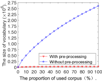
Figure 7: The growth of the vocabulary size.

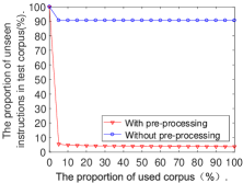
Figure 8: The proportion of unseen instructions.

We next investigate the number of OOV cases, i.e., unseen instructions, in later instruction embedding generation. We select two binaries that have never appeared in the previous corpus, containing 67,862 blocks and 453,724 instructions. We then count the percentage of unseen instructions that do not exist in the vocabulary, and show the result in Figure 8. The red and blue lines show the percentage of unseen instructions when the vocabulary is built with or without pre-processing, respectively. We can see that after pre-processing, only 3.7% unseen instructions happen in later instruction embedding generation, compared to 90% without pre-processing; (for an OOV instruction, a zero vector is assigned). This shows that the instruction embedding model with pre-processing has a good coverage of instructions. Thus, it may be reused by other researchers and we have made it publicly available.

VII-D Qualitative Analysis of Instruction Embeddings

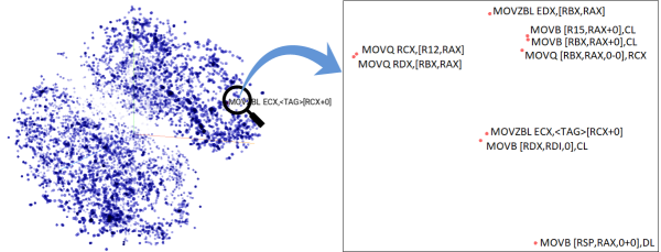
Figure 9: Visualization of all the instructions for x86 and ARM in 3D space, and a particular x86 instruction and its neighbor instructions, with t-SNE.

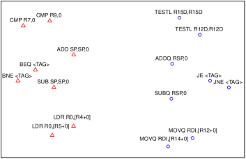
Figure 10: Visualization of a set of instructions for x86 and ARM based on MDS. The blue circles and red triangles represent x86 instructions and ARM instructions, respectively.

We present our results from qualitatively analyzing the instruction embeddings for the two architectures, x86 and ARM. We first use t-SNE [41], a useful tool for visualizing high-dimensional vectors, to plot the instruction embeddings in a three-dimensional space, as shown in Figure 10. A quick inspection immediately shows that the instructions compiled for the same architecture cluster together. Thus the most significant factor that influences code is the architecture as it introduces more syntactic variation. This also reveals one of the reasons why cross-architecture code similarity detection is more difficult than single-architecture code similarity detection.

We then zoom in Figure 10, and plot a particular x86 instruction MOVZBL EXC,<TAG>[RCX+0] and its neighbors. We can see that the mov family instructions are close together.

Next, we use the analogical reasoning to evaluate the quality of the cross-architecture instruction embedding model. To do this, we randomly pick up eight x86 instructions. For each x86 instruction, we select its similar counterpart from ARM based on our prior knowledge and experience. We use [$x$] and {$y$} to represent the embedding of an ARM instruction $x$, and an x86 instruction $y$, respectively; and cos([$x_{1}$], [$x_{2}$]) refers to the cosine distance between two ARM instructions, $x_{1}$ and $x_{2}$. We have the following findings: (1) cos([ADD SP,SP,0], [SUB SP,SP,0]) is approximate to cos({ADDQ RSP,0}, {SUBQ RSP,0}). (2) cos([ADD SP,SP,0], {ADDQ RSP,0}) is approximate to cos([SUB SP,SP,0], {SUBQ RSP,0}). This is similar to other instruction pairs. We plot the relative positions of these instructions in Figure 10 according to their cosine distance matrix based on MDS. We limit the presented examples to eight due to space limitation. In our manual investigation, we find many such semantic analogies that are automatically learned. Therefore, it shows that the instruction embedding model learns semantic information of instructions.

VII-E Accuracy of InnerEye-BB

We now evaluate the accuracy of our InnerEye-BB. All evaluations in this subsection are conducted on Dataset I.

VII-E1 Model Training

We divide Dataset I into three parts for training, validation, and testing: for similar basic-block pairs, 80% of them are used for training, 10% for validation, and the remaining 10% for testing; the same splitting rule is applied to the dissimilar block pairs as well. Table I shows the statistic results. In total, we have four training datasets: the first three datasets contain the basic-block pairs compiled with the same optimization level (O1, O2, and O3), and the last one contains the basic-block pairs with each one compiled with a different optimization level (cross-opt-levels). Note that in all the datasets, the two blocks of each pair are compiled for different architectures. This is the same for validation and testing datasets. Note that we make sure the training, validation, and testing datasets contain disjoint sets of basic blocks (we split basic blocks into three disjoint sets before constructing similar/dissimilar basic block pairs). Thus, any given basic block that appears in the training dataset does not appear in the validation or testing dataset. Through this, we can better examine whether our model can work for unseen blocks. Note that the instruction embedding matrices for different architectures can be precomputed and reused.

We use the four training datasets to train InnerEye-BB individually for 100 epochs. After each epoch, we measure the AUC and loss on the corresponding validation datasets, and save the models achieving the best AUC as the base models.

VII-E2 Results

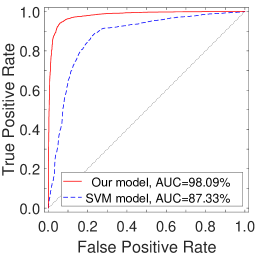
(a) O1

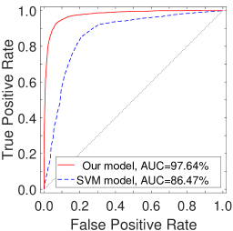
(b) O2

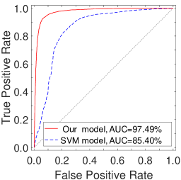
(c) O3

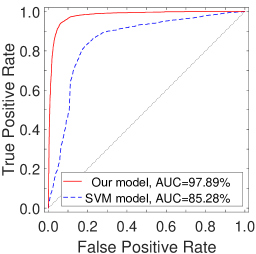
(d) Cross-opt-levels

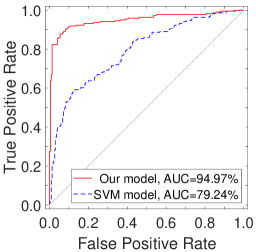
(e) Large basic blocks in O3

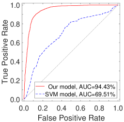
(f) Small basic blocks in O3

Figure 11: The ROC evaluation results based on the four testing datasets.

We now evaluate the accuracy of the base models using the corresponding testing datasets. The red lines in the first four figures in Figure 11, from (a) to (d), are the ROC curves of the similarity test. As each curve is close to the left-hand and top border, our models have good accuracy.

To further comprehend the performance of our models on basic blocks with different sizes, we create small-BB and large-BB testing subsets. If a basic block contains less than 5 instructions it belongs to the small-BB subset; a block containing more than 20 instructions belongs to the large-BB subset. We then evaluate the corresponding ROC. Figure 11e and Figure 11f show the ROC results evaluated on the large-BB subset (221 pairs) and small-BB subset (2409 pairs), respectively, where the basic-block pairs are compiled with the O3 optimization level. The ROC results evaluated on the basic-block pairs compiled with other optimization levels are similar, and are omitted here due to the page limit. We can observe that our models achieve good accuracy for both small blocks and large ones. Because a small basic block contains less semantic information, the AUC (=94.43%) of the small-BB subset (Figure 11f) is slightly lower than others. Moreover, as there are a small portion (4.4%) of large BB pairs in the training dataset, the AUC (=94.97%) of the large-BB subset (Figure 11e) is also slightly lower; we expect this could be improved if more large BB pairs are seen during training.

VII-E3 Comparison with Manually Selected Features

Several methods are proposed for cross-architecture basic block similarity detection, e.g., fuzzing [52], symbolic execution [21, 37], and basic-block feature-based machine learning classifier [19]. Fuzzing and symbolic execution are much slower than our deep learning based approach. We thus compare our model against the SVM classifier using six manually selected block features adopted in Gemini, such as the number of instructions and the number of constants (see Table 1 in  [65].

We extract the six features from each block to represent the block, and use all blocks in the training dataset to train the SVM classifier. We adopt leave-one-out cross-validation with $K=5$ and use the Euclidean distance to measure the similarity of blocks. By setting the complexity parameter $c=1.0$, $\gamma=1.0$ and choosing the RBF kernel, the SVM classifier achieves the best AUC value. Figure 11 shows the comparison results on different testing subsets. We can see that our models outperform the SVM classifier and achieve much higher AUC values. This is because the manually selected features largely lose the instruction semantics and dependency information, while InnerEye-BB precisely encodes the block semantics.

Examples. Table III shows three pairs of similar basic-block pairs (after pre-processing) that are correctly classified by InnerEye-BB, but misclassified by the statistical feature-based SVM model. Note that the pre-processing does not change the statistical features of basic blocks; e.g., the number of transfer instructions keeps the same before and after pre-processing. Our model correctly reports each pair as similar.

Table III shows three pairs of dissimilar basic-block pairs (after pre-processing) that are correctly classified by InnerEye-BB, but misclassified by the SVM model. As the statistical features of two dissimilar blocks tend to be similar, the SVM model—which ignores the meaning of instructions and the dependency between them—misclassifies them as similar.

TABLE II: Examples of similar BB pairs that are correctly classified by InnerEye-BB, but misclassified by the SVM model.

Pair 1		Pair 2		Pair 3
x86	ARM	x86	ARM	x86	ARM
MOVSLQ RSI,EBP	LDRB R0,[R8+R4]	MOVQ RDX,<TAG>+[RIP+0]	LDR R2,[R8+0]	MOVQ [RSP+0],RBX	LDR R0,[SP+0]
MOVZBL ECX,[R14,RBX]	STR R9,[SP]	MOVQ RDI,R12	MOV R0,R4	MOVQ [RSP+0],R14	STR R9,[SP+0]
MOVL EDX,<STR>	STR R0,[SP+0]	MOVL ESI,R14D	MOV R1,R5	ADDQ RDI,0	STR R0,[SP+0]
XORL EAX,EAX	ASR R3,R7,0	CALLQ FOO	BL FOO	CALLQ FOO	ADD R0,R1,0
MOVQ RDI,R13	MOV R0,R6	MOVQ RDI,R12	MOV R0,R4	MOVL ESI,<TAG>	BL FOO
CALLQ FOO	MOV R2,R7	CALLQ FOO	BL FOO	MOVQ RDI,[R12]	LDR R7,<TAG>
TESTL EAX,EAX	BL FOO	MOVQ RDX,<TAG>+[RIP+0]	LDR R2,[R8+0]	MOVB [RDI+0],AL	LDR R1,[R6]
JLE <TAG>	CMP R0,0	MOVQ RDI,R12	MOV R0,R4	CMPB [RDI+0],0	LDR LR,[SP+0]
	BLT <TAG>	MOVL ESI,R14D	MOV R1,R5	JNE <TAG>	MOV R12,R7
		CALLQ FOO	BL FOO		STRB R0,[R1+0]
		TESTL EAX,EAX	CMP R0,0		B <TAG>
		JNE <TAG>	BNE<TAG>

TABLE III: Examples of dissimilar BB pairs that are correctly classified by InnerEye-BB, but misclassified by the SVM model.

Pair 4		Pair 5		Pair 6
x86	ARM	x86	ARM	x86	ARM
IMULQ R13,RAX,0	MOV R1,R0	XORL R14D,R14D	LDMIB R5,R0,R1	MOVL [RSP+0],R14D	SUB R2,R1,0
XORL EDX,EDX	LDR R6,[SP+0]	TESTQ RBP,RBP	CMP R0,R1	MOVQ RAX,[RSP+0]	MOV R10,0
MOVQ RBP,[RSP+0]	CMP R0, 0	JE <TAG>	BHS <TAG>	CMPB [RAX],0	CMP R2,0
DIVQ RBP	BEQ <TAG>			MOVQ [RSP+0],R13	MOV R9,0
JMP <TAG>				MOVQ [RSP+0],R15	BHI <TAG>
				JNE <TAG>

VII-F Hyperparameter Selection for InnerEye-BB

We next investigate the impact of different hyperparameters on InnerEye-BB. In particular, we consider the number of epochs, the dimensionality of the embeddings, network depth, and hidden unit types. We use the validation datasets of Dataset I to examine the impact of the number of epochs, and the testing datasets to examine the impact of other hyperparameters.

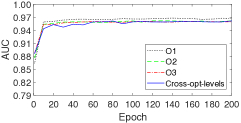
(a) AUC vs. # of epochs.

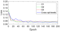
(b) Loss vs. # of epochs.

(%)	Optimization levels			Cross
	O1	O2	O3	-opts
50	95.77	95.23	94.97	95.39
100	96.83	96.33	95.99	95.82
150	96.89	96.33	96.24	95.86

(c) AUC vs. instruction embedding dimensions.

(%)	Optimization levels			Cross
	O1	O2	O3	-opts
10	95.57	95.73	95.48	95.59
30	95.88	95.65	96.17	95.45
50	96.83	96.33	95.99	95.82

(d) AUC vs. block embedding dimensions.

(%)	Optimization levels			Cross
	O1	O2	O3	-opts
1	95.88	95.65	96.17	95.45
2	97.83	97.49	97.59	97.45
3	98.16	97.39	97.48	97.76

(e) AUC vs. # of network layers.

(%)	Optimization levels			Cross
	O1	O2	O3	-opts
LSTM	96.83	96.33	95.99	95.82
GRU	96.15	95.30	95.83	95.71
RNN	91.39	93.26	92.60	92.66

(f) AUC vs. network hidden unite types.

Figure 12: Impact of different hyperparameters. Figure 12a and Figure 12b are evaluated on the validation datasets of Dataset I, and others are evaluated on its testing datasets.

VII-F1 Number of Epochs

To see whether the accuracy of the model fluctuates during training, we trained the model for 200 epochs and evaluated the model every 10 epochs for the AUC and loss. The results are displayed in Figure 12a and Figure 12b. We observe that the AUC value steadily increases and is stabilized at the end of epoch 20; and the loss value decreases quickly and almost stays stable after 20 epochs. Therefore, we conclude that the model can be quickly trained to achieve good performance.

VII-F2 Embedding Dimensions

We next measure the impact of the instruction embedding and block embedding dimensions.

Instruction embedding dimension. We vary the instruction embedding dimension, and evaluate the corresponding AUC values shown in Figure 12c. We observe that increasing the embedding dimensions yields higher performance; and the AUC values corresponding to the embedding dimension higher than 100 are close to each other. Since a higher embedding dimension leads to higher computational costs (requiring longer training time), we conclude that a moderate dimension of 100 is a good trade-off between precision and efficiency.

Block embedding dimension. Next, we vary the block embedding dimension, and evaluate the corresponding AUC values shown in Figure 12d. We observe that the performance of the models with 10, 30 and 50 block embedding dimensions are close to each other. Since a higher embedding dimension leads to higher computational costs, we conclude that a dimension of 50 for block embeddings is a good trade-off.

VII-F3 Network Depth

We then change the number of layers of each LSTM, and evaluate the corresponding AUC values. Figure 12e shows that the LSTM networks with two and three layers outperform the network with a single layer, and the AUC values for the networks with two and three layers are close to each other. Because adding more layers increases the computational complexity and does not help significantly on the performance, we choose the network depth as 2.

VII-F4 Network Hidden Unit Types

As a simpler-version of LSTM, Gated Recurrent Unit (GRU) has become increasingly popular. We conduct experiments on comparing three types of network units, including LSTM, GRU as well as RNN. Figure 12f shows the comparison results. It can be seen that LSTM and GRU are more powerful than the basic RNN, and LSTM shows the highest AUC values.

VII-G Efficiency of InnerEye-BB

VII-G1 Training Time

We first analyze the training time for both the instruction and basic-block embedding models.

Instruction embedding model training time. The training time is linear to the number of epochs and the corpus size. We use Dataset I, containing 437,104 blocks for x86 and 393,529 blocks for ARM, with 6,199,651 instructions in total, as the corpus to train the instruction embedding model. The corpus contains 49,760 distinct instructions which form a vocabulary. We use $10^{-5}$ as the down sampling rate and set the parameter mini-word-count as zero (no word is ignored during training), and train the model for 100 epochs. Table IV shows the training time with respect to different instruction embedding dimensions. We can see that the instruction embedding model can be trained in a very short period of time.

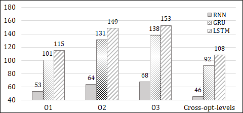
(a) Training time of single-layer networks with respect to different hidden unit types.

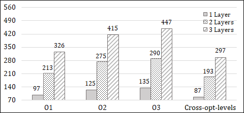
(b) Training time of LSTMs with respect to different number of network layers

Figure 13: Training time of the basic-block embedding model. The instruction embedding dimension is 100, and the block embedding dimension is 50. The number above each bar is the time (second per epoch) used to train the model.

(Second)	Optimization levels			Cross
	O1	O2	O3	-opts
L=1, D=30	3.040	3.899	4.137	2.944
L=1, D=50	3.530	4.702	4.901	3.487
L=2, D=30	6.359	8.237	8.780	6.266
L=2, D=50	6.663	8.722	9.139	6.625

Figure 14: Testing time of InnerEye-BB with respect to different number of network layers and block embedding dimensions. The instruction embedding dimension is 100. $L$ denotes the number of network layers. $D$ denotes the block embedding dimension.

Block embedding model training time. We next evaluate the time used for training the basic-block embedding model. The training time is linear to the number of epochs and the number of training samples. The results are showed in Figure 14. The number above each bar is the time (second per epoch) used to train the model. Figure 13a shows the training time with respect to different types of network hidden unit. Figure 13b displays the training time of the LSTM networks in terms of different number of network layers. In general, LSTM takes longer training time, and a more complicated model (with more layers) requires more time per epoch.

TABLE IV: Training time of the instruction embedding model with respect to different embedding dimensions.

Instruction embedding dimension	50	100	150
Training time (second)	82.71	84.22	89.75

Earlier we have shown that the block embedding model with 2 network layers and 20 epochs of training can achieve a good performance (Section VII-F), which means that it requires five and a half hours (=$(213+275+290+193)\times 20/3600$) to train the four models on the four training subsets, and each model takes around an hour and a half for training. With a single network layer, each model only needs about 40 mins for training and can still achieve a good performance.

VII-G2 Testing Time

We next investigate the testing time of InnerEye-BB. We are interested in the impacts of the number of network layers and the dimension of block embeddings, in particular. Figure 14 summaries the similarity test on the four testing datasets in Dataset I. The result indicates that the number of network layers is the major contributing factor of the computation time. Take the second column as an example. For a single-layer LSTM network with the block embedding dimension as 50, it takes 0.41 ms ($=3.530/8722$) on average to measure the similarity of two blocks, while a double-layer LSTM network requires 0.76 ms ($=6.663/8722$) on average.

Comparison with Symbolic Execution. We compare the proposed embedding model with one previous basic-block similarity comparison tool which relies on symbolic execution and theorem proving [37]. We randomly select 1,000 block pairs and use the symbolic execution-based tool to measure the detection time for each pair. The result shows that the InnerEye-BB runs 3700x to 140000x faster, and the speedup can be as high as 8000x on average.

The reason for the high efficiency of our model is that most computations of InnerEye-BB are implemented as easy-to-compute matrix operations (e.g., matrix multiplication, matrix summation, and element-wise operations over a matrix). Moreover, such operations can be parallelized to utilize multi-core CPUs or GPUs to achieve further speedup.

VII-H Code Component Similarity Comparison

We conduct three case studies to demonstrate how InnerEye-CC can handle real-world programs for cross-architecture code component similarity detection.

VII-H1 Thttpd

This experiment evaluated thttpd (v2.25b) and sthttpd (v2.26.4), where sthttpd is forked from thttpd for maintenance. Thus, their codebases are similar, with many patches and new building systems added to sthttpd. To measure false positives, we tested our tool on four independent programs, including thttpd (v2.25b), atphttpd (v0.4b), boa (v0.94.13), and lighttpd (v1.4.30). We use two architectures (x86 and ARM) and clang with different compiler optimization levels (O1-O3) to compile each program.

We consider a part of the httpd_parse_request function as well as the functions invoked within this code part from thttpd as the query code component, and check whether it is reused in sthttpd. Such code part checks for HTTP/1.1 absolute URL and is considered as critical. We first identify the starting blocks both in the query code component and the target program sthttpd (Section VI-B), and proceed with the path exploration to calculate the similarity score, which is 91%, indicating that sthttpd reuses the query code component. The whole process is finished within 2 seconds. However, CoP [37] (it uses symbolic execution and theorem proving to measure the block similarity) takes almost one hour to complete. Thus, by adopting techniques in NMT to speed up block comparison, InnerEye  is more efficient and scalable.

To measure false positives, we test InnerEye against four independently developed programs. We use the query code component to search for the similar code components in atphttpd (v0.4b), boa (v0.94.13), and lighttpd (v1.4.30). Very low similarity scores (below 4%) are reported, correctly indicating that these three programs do not reuse the query code component.

VII-H2 Cryptographic Function Detection

We next apply InnerEye to the cryptographic function detection task. We choose MD5 and AES as the query functions, and search for their implementations in 13 target programs ranging from small to large real-world software, including cryptlib (v3.4.2), OpenSSL (v1.0.1f), openssh (v6.5p1), git (v1.9.0), libgcrypt (v1.6.1), truecrypt (v7.1a), berkeley DB (v6.0.30), MySQL (v5.6.17), glibc (v2.19), p7zip (v9.20.1), cmake (v2.8.12.2), thttpd (v2.25b), and sthttpd (v2.26.4). We use x86 and ARM, and clang with O1–O3 optimization levels to compile each program.

MD5. MD5 is a cryptographic hash function that produces a 128-bit hash value. We first extract the implementation of MD5 from OpenSSL compiled targeting x86 with -O2. The part of the MD5 code that implements message compressing is selected as the query.

We use the query code component to search for similar code components from the target programs. The results show that cryptlib, openssh, libgcrypt, MySQL, glibc, and cmake implement MD5 with similarity scores between 88% and 93%. We have checked the source code and confirmed it.

AES. AES is a 16-byte block cipher and processes input via a substitution-permutation network. We extract the implementation of AES from OpenSSL compiled for ARM with -O2, and select a part of the AES code that implements transformation iterations as the query code component.

We test the query code component to check whether it is reused in the target programs, and found that cryptlib, openssh, libgcrypt, truecrypt, berkeley DB, and MySQL contain AES with the similarity scores between 86% and 94%, and the others do not. We have checked the source code and obtained consistent results.

The case studies demonstrate that InnerEye-CC is an effective and precise tool for cross-architecture binary code component similarity detection.

VIII Discussion

We chose to modify LLVM to prepare similar/dissimilar basic blocks, as LLVM is well structured as passes and thus it is easier to add the basic block boundary annotator to LLVM than GCC. However, the presented model merely learned from binaries compiled by LLVM. We have not evaluated how well our model can be used to analyze binaries in the case binaries are compiled using diverse compilers. As word embeddings and LSTM are good at extracting instruction semantics and their dependencies, we believe our approach itself is compiler-agnostic. We will verify this point in our future work.

We evaluated our tool on its tolerability of the syntactic variation introduced by different architectures and compiling settings; but we have not evaluated the impact of code obfuscation. How to handle obfuscations on the basic block level without relying on expensive approaches such as symbolic execution is a challenging and important problem. We plan to explore, with plenty of obfuscated binary basic blocks in the training dataset, whether the presented model can handle obfuscations by properly capturing the semantics of binary basic blocks. But it is notable that, at the program path level, our system inherits the powerful capability of handling obfuscations due to, e.g., garbage code insertion and opaque predicate insertion, from CoP [37].

Finally, it is worth pointing out that, as many prior systems are built on basic block comparison or representation [21, 44, 37, 52, 19], they can benefit from our block embedding model, which provides precise and efficient basic block information extraction and comparison.

IX Conclusion

Inspired by Neural Machine Translation, which is able to compare the meanings of sentences of different languages, we propose a novel neural network-based basic-block similarity comparison tool InnerEye-BB by regarding instructions as words and basic block as sentences. We thus borrow techniques from NMT: word embeddings are used to represent instructions and then LSTM is to encode both instruction embeddings and instruction dependencies. It is the first tool that achieves both efficiency and accuracy for cross-architecture basic-block comparison; plus, it does not rely on any manually selected features. By leveraging InnerEye-BB, we propose the first tool InnerEye-CC that resolves the cross-architecture code containment problem. We have implemented the system and performed a comprehensive evaluation. This research successfully demonstrates that it is promising to approach binary analysis from the angle of language processing by adapting methodologies, ideas and techniques in NLP.

References

- [1] M. Abadi, P. Barham, J. Chen, Z. Chen, A. Davis, J. Dean, M. Devin, S. Ghemawat, G. Irving, M. Isard et al., “Tensorflow: A system for large-scale machine learning.” in OSDI, 2016.
- [2] B. S. Baker, “On finding duplication and near-duplication in large software systems,” in WCRE, 1995.
- [3] BAP: The Next-Generation Binary Analysis Platform, “http://bap.ece. cmu.edu/,” 2013.
- [4] Y. Bengio, R. Ducharme, P. Vincent, and C. Jauvin, “A neural probabilistic language model,” Journal of Machine Learning Research, vol. 3, no. Feb, pp. 1137–1155, 2003.
- [5] M. Bilenko and R. J. Mooney, “Adaptive duplicate detection using learnable string similarity measures,” in KDD, 2003.
- [6] J. Bromley, I. Guyon, Y. LeCun, E. Säckinger, and R. Shah, “Signature verification using a "Siamese" time delay neural network,” in NIPS, 1994.
- [7] D.-K. Chae, S.-W. Kim, J. Ha, S.-C. Lee, and G. Woo, “Software plagiarism detection via the static API call frequency birthmark,” in Annual ACM Symposium on Applied Computing (SAC), 2013.
- [8] M. Chandramohan, Y. Xue, Z. Xu, Y. Liu, C. Y. Cho, and H. B. K. Tan, “BinGo: Cross-architecture cross-OS binary search,” in FSE, 2016.
- [9] F. Chollet et al., “Keras,” https://keras.io, 2015.
- [10] S. Chopra, R. Hadsell, and Y. LeCun, “Learning a similarity metric discriminatively, with application to face verification,” in CVPR, 2005.
- [11] Z. L. Chua, S. Shen, P. Saxena, and Z. Liang, “Neural nets can learn function type signatures from binaries,” in USENIX Security, 2017.
- [12] J. Chung, C. Gulcehre, K. Cho, and Y. Bengio, “Empirical evaluation of gated recurrent neural networks on sequence modeling,” in NIPS Deep Learning and Representation Learning Workshop, 2014.
- [13] J. Crussell, C. Gibler, and H. Chen, “Attack of the clones: Detecting cloned applications on android markets,” in ESORICS, 2012.
- [14] Y. David, N. Partush, and E. Yahav, “Statistical similarity of binaries,” in PLDI, 2016.
- [15] Y. David, N. Partush, and E. Yahav, “Similarity of binaries through re-optimization,” in PLDI, 2017.
- [16] S. Deerwester, S. T. Dumais, G. W. Furnas, T. K. Landauer, and R. Harshman, “Indexing by latent semantic analysis,” Journal of the American society for information science, vol. 41, no. 6, pp. 391–407, 1990.
- [17] S. H. Ding, B. C. Fung, and P. Charland, “Asm2vec: Boosting static representation robustness for binary clone search against code obfuscation and compiler optimization,” in IEEE Symposium on Security and Privacy (SP), 2019.
- [18] S. Eschweiler, K. Yakdan, and E. Gerhards-Padilla, “discovRE: Efficient cross-architecture identification of bugs in binary code.” in NDSS, 2016.
- [19] Q. Feng, R. Zhou, C. Xu, Y. Cheng, B. Testa, and H. Yin, “Scalable graph-based bug search for firmware images,” in CCS, 2016.
- [20] M. Gabel, L. Jiang, and Z. Su, “Scalable detection of semantic clones,” in ICSE, 2008.
- [21] D. Gao, M. Reiter, and D. Song, “Binhunt: Automatically finding semantic differences in binary programs,” in ICICS, 2008.
- [22] Gartner says 8.4 billion connected "Things" will be in use in 2017, “http://www.gartner.com/newsroom/id/3598917,” 2017.
- [23] Z. Han, X. Li, Z. Xing, H. Liu, and Z. Feng, “Learning to predict severity of software vulnerability using only vulnerability description,” in International Conference on Software Maintenance and Evolution (ICSME), 2017.
- [24] S. Hochreiter and J. Schmidhuber, “Long short-term memory,” Neural computation, vol. 9, no. 8, pp. 1735–1780, 1997.
- [25] X. Huo and M. Li, “Enhancing the unified features to locate buggy files by exploiting the sequential nature of source code,” in IJCAI, 2017.
- [26] X. Huo, M. Li, and Z.-H. Zhou, “Learning unified features from natural and programming languages for locating buggy source code.” in IJCAI, 2016.
- [27] Y.-C. Jhi, X. Wang, X. Jia, S. Zhu, P. Liu, and D. Wu, “Value-based program characterization and its application to software plagiarism detection,” in ICSE, 2011.
- [28] L. Jiang, G. Misherghi, Z. Su, and S. Glondu, “Deckard: Scalable and accurate tree-based detection of code clones,” in ICSE, 2007.
- [29] N. Kalchbrenner and P. Blunsom, “Recurrent continuous translation models.” in EMNLP, 2013.
- [30] N. Kalchbrenner, E. Grefenstette, and P. Blunsom, “A convolutional neural network for modelling sentences,” in CIKM, 2013.
- [31] T. Kamiya, S. Kusumoto, and K. Inoue, “CCFinder: A multilinguistic token-based code clone detection system for large scale source code,” IEEE Transactions on Software Engineering, 2002.
- [32] R. Koschke, R. Falke, and P. Frenzel, “Clone detection using abstract syntax suffix trees,” in WCRE, 2006.
- [33] Q. Le and T. Mikolov, “Distributed representations of sentences and documents,” in ICML, 2014.
- [34] J. Li and M. D. Ernst, “CBCD: Cloned buggy code detector,” in ICSE, 2012.
- [35] B. Liu, W. Huo, C. Zhang, W. Li, F. Li, A. Piao, and W. Zou, “Diff: cross-version binary code similarity detection with DNN,” in ASE, 2018.
- [36] C. Liu, C. Chen, J. Han, and P. S. Yu, “GPLAG: detection of software plagiarism by program dependence graph analysis,” in KDD, 2006.
- [37] L. Luo, J. Ming, D. Wu, P. Liu, and S. Zhu, “Semantics-based obfuscation-resilient binary code similarity comparison with applications to software plagiarism detection,” in FSE, 2014.
- [38] L. Luo, J. Ming, D. Wu, P. Liu, and S. Zhu, “Semantics-based obfuscation-resilient binary code similarity comparison with applications to software and algorithm plagiarism detection,” IEEE Transactions on Software Engineering, no. 12, pp. 1157–1177, 2017.
- [39] L. Luo and Q. Zeng, “SolMiner: mining distinct solutions in programs,” in ICSE-C, 2016.
- [40] L. Luo, Q. Zeng, C. Cao, K. Chen, J. Liu, L. Liu, N. Gao, M. Yang, X. Xing, and P. Liu, “System service call-oriented symbolic execution of android framework with applications to vulnerability discovery and exploit generation,” in Proceedings of the 15th Annual International Conference on Mobile Systems, Applications, and Services. ACM, 2017, pp. 225–238.
- [41] L. v. d. Maaten and G. Hinton, “Visualizing data using t-SNE,” Journal of Machine Learning Research, vol. 9, no. Nov, pp. 2579–2605, 2008.
- [42] T. Mikolov, K. Chen, G. Corrado, and J. Dean, “Efficient estimation of word representations in vector space,” in ICLR Workshop, 2013.
- [43] T. Mikolov, I. Sutskever, K. Chen, G. S. Corrado, and J. Dean, “Distributed representations of words and phrases and their compositionality,” in NIPS, 2013.
- [44] J. Ming, M. Pan, and D. Gao, “iBinHunt: Binary hunting with inter-procedural control flow,” in Annual International Conference on Information Security and Cryptology (ICISC), 2012.
- [45] J. Ming, F. Zhang, D. Wu, P. Liu, and S. Zhu, “Deviation-based obfuscation-resilient program equivalence checking with application to software plagiarism detection,” IEEE Transactions on Reliability, 2016.
- [46] S. A. Mokhov, J. Paquet, and M. Debbabi, “The use of NLP techniques in static code analysis to detect weaknesses and vulnerabilities,” in Canadian Conference on Artificial Intelligence, 2014.
- [47] L. Mou, G. Li, L. Zhang, T. Wang, and Z. Jin, “Convolutional neural networks over tree structures for programming language processing.” in AAAI, 2016.
- [48] J. Mueller and A. Thyagarajan, “Siamese recurrent architectures for learning sentence similarity,” in AAAI, 2016.
- [49] T. D. Nguyen, A. T. Nguyen, H. D. Phan, and T. N. Nguyen, “Exploring API embedding for API usages and applications,” in ICSE, 2017.
- [50] H. Palangi, L. Deng, Y. Shen, J. Gao, X. He, J. Chen, X. Song, and R. Ward, “Deep sentence embedding using long short-term memory networks: Analysis and application to information retrieval,” IEEE/ACM Transactions on Audio, Speech and Language Processing (TASLP), 2016.
- [51] H. Park, S. Choi, H.-i. Lim, and T. Han, “Detecting code theft via a static instruction trace birthmark for Java methods,” in International Conference on Industrial Informatics (INDIN), 2008.
- [52] J. Pewny, B. Garmany, R. Gawlik, C. Rossow, and T. Holz, “Cross-architecture bug search in binary executables,” in IEEE Symposium on Security and Privacy (SP), 2015.
- [53] J. Pewny, F. Schuster, L. Bernhard, T. Holz, and C. Rossow, “Leveraging semantic signatures for bug search in binary programs,” in ACSAC, 2014.
- [54] L. Prechelt, G. Malpohl, and M. Philippsen, “Finding plagiarisms among a set of programs with JPlag,” Journal of Universal Computer Science, vol. 8, no. 11, pp. 1016–1038, 2002.
- [55] S. Schleimer, D. S. Wilkerson, and A. Aiken, “Winnowing: local algorithms for document fingerprinting,” in SIGMOD, 2003.
- [56] D. Schuler, V. Dallmeier, and C. Lindig, “A dynamic birthmark for Java,” in ASE, 2007.
- [57] I. Sutskever, O. Vinyals, and Q. V. Le, “Sequence to sequence learning with neural networks,” in NIPS, 2014.
- [58] H. Tamada, K. Okamoto, M. Nakamura, A. Monden, and K.-i. Matsumoto, “Dynamic software birthmarks to detect the theft of windows applications,” in International Symposium on Future Software Technology, 2004.
- [59] Z. Tian, Q. Zheng, T. Liu, and M. Fan, “DKISB: Dynamic key instruction sequence birthmark for software plagiarism detection,” in HPCC_EUC, 2013.
- [60] X. Wang, Y.-C. Jhi, S. Zhu, and P. Liu, “Behavior based software theft detection,” in CCS, 2009.
- [61] X. Wang, Y.-C. Jhi, S. Zhu, and P. Liu, “Detecting software theft via system call based birthmarks,” in ACSAC, 2009.
- [62] A. H. Watson and T. J. McCabe, Structured testing: A testing methodology using the cyclomatic complexity metric. US Department of Commerce, Technology Administration, NIST, 1996, vol. 500, no. 235.
- [63] M. White, M. Tufano, M. Martinez, M. Monperrus, and D. Poshyvanyk, “Sorting and transforming program repair ingredients via deep learning code similarities,” arXiv preprint: 1707.04742, 2017.
- [64] J. Wieting, M. Bansal, K. Gimpel, and K. Livescu, “Towards universal paraphrastic sentence embeddings,” in ICLR, 2016.
- [65] X. Xu, C. Liu, Q. Feng, H. Yin, L. Song, and D. Song, “Neural network-based graph embedding for cross-platform binary code similarity detection,” in CCS, 2017.
- [66] F. Zhang, D. Wu, P. Liu, and S. Zhu, “Program logic based software plagiarism detection,” in International Symposium on Software Reliability Engineering (ISSRE), 2014.