Efficient Sum-of-Sinusoids based Spatial Consistency for the 3GPP New-Radio Channel Model

Abstract

Spatial consistency was proposed in the 3GPP TR 38.901 channel model to ensure that closely spaced mobile terminals have similar channels. Future extensions of this model might incorporate mobility at both ends of the link. This requires that all random variables in the model must be correlated in 3 (single-mobility) and up to 6 spatial dimensions (dual-mobility). Existing filtering methods cannot be used due to the large requirements of memory and computing time. The sum-of-sinusoids model promises to be an efficient solution. To use it in the 3GPP channel model, we extended the existing model to a higher number of spatial dimensions and propose a new method to calculate the sinusoid coefficients in order to control the shape of the autocorrelation function. The proposed method shows good results for 2, 3, and 6 dimensions and achieves a four times better approximation accuracy compared to the existing model. This provides a very efficient implementation of the 3GPP proposal and enables the simulation of many communication scenarios that were thought to be impossible to realize with geometry-based stochastic channel models.

I Introduction

Channel models are an essential requirement for the development of new wireless communication protocols and systems. Standardized channel models can be used to evaluate and compare the different proposals against each other. For the upcoming fifth generation (5G) of wireless cellular communications, a new channel model was proposed by the 3rd generation partnership project (3GPP) [1]. An open-source implementation of this model is provided by the quasi deterministic radio channel generator (QuaDRiGa) [2, 3]. An essential new feature that was introduced by 3GPP is spatial consistency which solves one major drawback of previous geometry-based stochastic channel models (GSCMs), namely the lack of realistic correlation in the small-scale-fading (SSF). Without spatial consistency, the positions of individual scattering clusters are generated randomly for each new mobile terminal (MT) position. This contradicts the causality and the observations made in channel measurements [4].

GSCMs consist of two main components: a stochastic part that generates a random propagation environment, and a deterministic part that lets transmitters and receivers interact with this environment. In order to make realistic predictions of the wireless system performance, the random environment must fulfill certain statistical properties which are determined by measurements. This means that for a given set of model parameters the joint spatial correlation of these parameters must be captured for a large number of transceivers. This is done in the so-called large-scale fading (LSF) model. A subsequent SSF model then generates individual scattering clusters for each MT.

Large-scale parameters (LSPs) are more or less constant within an area of several meters. An example for this is the shadow fading (SF) which is caused by buildings or trees blocking a significant part of the signal. The so-called decorrelation distance of the SF, i.e., the distance a MT must move to experience a significant change in the SF, is in the same order of magnitude as the size of the objects causing it. Thus, if a MT travels along a trajectory or if multiple MTs are closely spaced together, their LSPs are correlated. A common approach to model such correlation is by filtered Gaussian-distributed random numbers [5]. However, when it comes to spatial consistency, the positions of the scattering clusters must also be spatially correlated. The 3GPP proposal suggests that “spatially consistent powers/delays/angles of clusters are generated” [1]. However, this requires that all random variables that determine the location of the scattering clusters are correlated. For a moderate scenario with 12 clusters and 20 sub-paths per cluster, this results in 2288 random variables. Compared to the 7 variables needed for the LSF model, the filtering approach therefore requires a prohibitively large amounts of memory and computing time.

Another problem arises when incorporating so-called vertical industries into the 5G infrastructure which is not yet covered by the 3GPP new-radio model but discussed in several ongoing research projects and standardization activities. Such verticals could be vehicular networks, air-to-ground communications, industrial peer-to-peer (P2P) communications, or communication scenarios involving satellites in low-earth orbit. All of these examples have in common that both ends of the link are mobile. However, the simultaneous mobility of both communication partners is not supported by the classical cellular shadowing models. Therefore, an alternative method for the generation of the random propagation environment is needed [6].

A computational efficient method to generate correlated random variables has been introduced by Pätzold el. al. [7] who approximated the filtered white Gaussian noise process by a finite sum of properly weighted sinusoids. This idea was further developed into a two-dimensional (2-D) shadowing model [8]. Wang et. al. then extended this 2-D method into a four-dimensional (4-D) method for device-to-device (D2D) channels [9]. A common problem for all these methods is finding the coefficients that best approximate a desired autocorrelation function (ACF) with a limited number of sinusoids.

In this paper, a new approximation method is presented that allows the efficient calculation of the sinusoid coefficients for an arbitrary ACF in three-dimensional (3-D) space. Previously published results focused solely on the exponential ACF and mobility was limited to planar movements. Furthermore, it is shown how this translates directly into a six-dimensional random process for D2D channels where both ends can be in different propagation environments, such as in air-to-ground channels. Compared to [9], the proposed method also achieves a 6.5 dB better approximation average squared error (ASE) with the same number of sinusoids. An implementation of this model is available in MATLAB and Octave as part of the open-source QuaDRiGa channel model [3].

II The Sum of Sinusoids Model

A spatially correlated Gaussian random process generates Normal distributed random numbers

$$k(x,y,z)\sim\mathcal{N}(0,1)\text{,}$$ (1)

with zero mean and unit variance. The value $k$ is a function of the terminal location in 3-D Cartesian coordinates $(x,y,z)$. From these numbers, other types of distributions can be obtained, e.g. Uniform or log-Normal distributed random numbers having a different mean or variance. The one-dimensional (1-D) spatial autocorrelation function (ACF) describes how fast the local mean of $k(x,y,z)$ evolves as a terminal moves. The ACF is usually modeled as an exponential decay function

$$\rho(d)=\exp\left(-\frac{d}{d_{\lambda}}\right)\text{,}$$ (2)

with $d$ as the distance between two positions and $d_{\lambda}$ as the so-called decorrelation distance, i.e. the distance at which the correlation between two samples falls below $e^{-1}\approx 0.37$ [10]. However, other types of decay functions may be desirable. The sum-of-sinusoids (SOS) method outlined in [7] approximates a 1-D Gaussian random process $k(x)$ as a function of the position $x$ on a 1-D linear trajectory as

$$\hat{k}(x)=\sum_{n=1}^{N}a_{n}\cos\left\{2\pi f_{n}x+\psi_{n}\right\}$$ (3)

with $N$ sinusoids. The variables $a_{n}$, $f_{n}$, and $\psi_{n}$ denote the amplitude, the frequency, and the phase of a sinusoid, respectively. The amplitudes $a_{n}$ and the frequencies $f_{n}$ are determined in a way that $\hat{k}(x)$ has similar statistical properties as $k(x)$, i.e. $\hat{k}(x)$ has the same approximate ACF and the cumulative distribution function (CDF) is close to Gaussian density if $N$ is sufficiently large. According to [7], 6 to 30 sinusoids are sufficient for a 1-D approximation. The phases $\psi_{n}$ are random variables distributed in the range from $-\pi$ to $\pi$. Hence, exchanging the $\psi_{n}$ while keeping $a_{n}$ and $f_{n}$ fixed creates a new set of spatially correlated random variables at minimal computational cost. A straight-forward expansion to a 3-D Gaussian random process follows from [9] as

$$\hat{k}(x,y,z)=\sum_{n=1}^{N}a_{n}\cos\left\{2\pi\left(f_{x,n}x+f_{y,n}y+f_{z,n}z\right)+\psi_{n}\right\}\text{.}$$ (4)

Under the assumption that the fluctuations of $k(x,y,z)$ are wide sense stationary, the ACF only depends on the distance between two terminal positions. Hence, the 3-D spatial ACF of $\hat{k}(x,y,z)$ can be expressed as [9]

$$\hat{\rho}(\Delta x,\Delta y,\Delta z)=\\ \sum_{n=1}^{N}\frac{a_{n}^{2}}{2}\cos\left\{2\pi\left(f_{x,n}\Delta x+f_{y,n}\Delta y+f_{z,n}\Delta z\right)\right\}\text{.}$$ (5)

When a MT moves from one location to another, the correlation $\rho(\Delta x,\Delta y,\Delta z)$ between the generated values $k(x,y,z)$ depends not only on the distance, but also on the direction of movement. In 3-D space, the traveling direction can be expressed by pitch and yaw. The pitch angle $\theta$ describes the vertical (tilt) angle relative to the horizontal plane. Positive rotation is up. The bearing or yaw angle $\phi$ describes the orientation on the ground. Here, it is defined in mathematic sense, i.e., seen from above, a value of 0 points to the east and the angles increase counter-clockwise. By assigning a direction $(\theta_{n},\phi_{n})$ to each of the $N$ sinusoids, the relative movement in $x$, $y$, and $z$ direction can be expressed as

$$f_{x,n}\Delta x = f_{n}\cdot d\cdot\cos\phi_{n}\cos\theta_{n},$$ (6)

$$f_{y,n}\Delta y = f_{n}\cdot d\cdot\sin\phi_{n}\cos\theta_{n},$$ (7)

$$f_{z,n}\Delta z = f_{n}\cdot d\cdot\sin\theta_{n},$$ (8)

where $f_{n}$ is the root-frequency of the $n$-th sinusoid frequency and $d$ is the distance. The directions $(\theta_{n},\phi_{n})$ have to be chosen in a way that covers all possible movement directions of the MT. This can be done by generating equidistributed points on the surface of a sphere as described in [11].

Pätzold et. al. [7] proposed four methods to determine the amplitudes $a_{n}$ and frequencies $f_{n}$ in a SOS model. All of them show different performance in terms of average squared error (ASE) vs. the number of sinusoids, and computational complexity. They have in common that the approximated ACF is an exponential decay function (2). However, this is not always desirable since other types of decay functions might be needed. Hence, in the next section, a numeric approximation method is presented that calculates the sinusoid coefficients for arbitrary ACFs.

III Approximation of Arbitrary ACFs

The approximation method is derived from the Monte Carlo method [12, 7]. The sinusoid frequencies $f_{n}$ are generated by an iterative optimization method that minimizes the error between the desired ACF and the approximate ACF for a given number of sinusoids. This method requires that the ACF is discretely sampled at $s=1\ldots S$ sampling distances. This is done by defining a vector $\mathbf{d}$ that contains the sampling distances in increasing order.

$$\mathbf{d}=\left(\begin{array}[]{cccc}d_{1}&d_{2}&\ldots&d_{S}\\ \end{array}\right)^{T}$$ (9)

Then, the sampled ACF $\rho(\mathbf{d})$ is obtained. The first distance value $d_{1}$ must be 0 and the first correlation value $\rho_{1}$ must be 1, i.e. at zero-distance the generated values $\hat{k}(x,y,z)$ are identical. The $N$ root-frequencies are randomly initialized to

$$f_{n}\sim\frac{1}{d_{S}}\cdot\mathcal{U}(-\pi,\pi)\text{,}$$ (10)

where $\mathcal{U}(-\pi,\pi)$ describes an uniform distribution with values between $-\pi$ and $\pi$, and $d_{S}$ the maximum distance for which the ACF is defined. The directional components $f_{x,n}$, $f_{y,n}$, and $f_{z,n}$ are calculated according to (6), (7), and (8) with $d=\Delta x=\Delta y=\Delta z=1$, respectively.

The iterative optimization is done by updating the $n$-th root frequency while keeping all other $N-1$ frequencies fixed. Then, the ASE is calculated. If it improves, the update is applied, otherwise it is discarded and the previous value of $f_{n}$ is used. The update is calculated by

$$f_{n}=\frac{1}{d_{S}}\arg\min_{f}\sum_{s=1}^{S}\left\{\rho(d_{s})-\hat{\rho}(d_{s})-\frac{1}{N}\cos\left(\frac{2\pi}{d_{S}}fd_{s}\right)\right\}^{2}\text{,}$$ (11)

where $\rho(d_{s})$ is the desired ACF and $\hat{\rho}(d_{s})$ is the approximate ACF constructed from all $N-1$ components from the previous iteration. The amplitudes of all sinusoids are set to $a_{n}^{2}=\frac{2}{N}$ and standard numerical methods can be applied to find the values $f$. However, (11) can only be used to approximate a 1-D random process such as (3). For a 3-D random process (4) it is necessary to estimate the three sinusoid components $f_{x,n}$, $f_{y,n}$, and $f_{z,n}$. This can be done by performing the estimation along the axes of the coordinate system. For example, combining (6) and (5) while setting $\Delta y=\Delta z=0$ leads to a directional ACFs in $x$-direction

$$\hat{\rho}(\Delta x)=\frac{1}{N}\sum_{n=1}^{N}\cos(2\pi d_{s}\cdot\underbrace{f_{n}\cos\phi_{n}\cos\theta_{n}}_{=f_{x,n}})\text{.}$$ (12)

This function is used instead of $\hat{\rho}(d_{s})$ in (11) to get an update of the $n$-th root frequency $f_{n}$. Due to the linear dependency, $f_{x,n}$, $f_{y,n}$, and $f_{z,n}$ can be calculated from (6), (7), and (8). The same approach can be used to perform the estimation in $y$ or $z$-direction, where

$$\hat{\rho}(\Delta y) = \frac{1}{N}\sum_{n=1}^{N}\cos(2\pi d_{s}\cdot\underbrace{f_{n}\sin\phi_{n}\cos\theta_{n}}_{=f_{y,n}})\text{,}$$ (13)

$$\hat{\rho}(\Delta z) = \frac{1}{N}\sum_{n=1}^{N}\cos(2\pi d_{s}\cdot\underbrace{f_{n}\sin\theta_{n}}_{=f_{z,n}}).$$ (14)

Depending on which of the $N$ sinusoid frequencies is estimated, the estimation direction is chosen according to

$$\hat{\rho}(d_{s})=\left\{\begin{array}[]{ll}\hat{\rho}(\Delta x),&\hbox{for }\Delta x\geq\Delta y\hbox{ and }\Delta x\geq\Delta z\hbox{;}\\ \hat{\rho}(\Delta y),&\hbox{for }\Delta y>\Delta x\hbox{ and }\Delta y\geq\Delta z\hbox{;}\\ \hat{\rho}(\Delta z),&\hbox{for }\Delta z>\Delta x\hbox{ and }\Delta z>\Delta y\hbox{,}\end{array}\right.$$ (15)

where $\Delta x$, $\Delta y$, and $\Delta z$ are calculated according to (6), (7), and (8) with $d=1$, respectively.

Cai and Giannakis [8] introduced the ASE as a performance measure of the approximation. It is defined as the average squared error between the desired ACF $\rho(\mathbf{d})$ and the approximate ACF $\hat{\rho}(\Delta x,\Delta y,\Delta z)$. Here it is calculated as

$$\mathrm{ASE}=\frac{1}{ST}\sum_{t=1}^{T}\sum_{s=1}^{S}\left\{\rho(d_{s})-\frac{1}{N}\sum_{n=1}^{N}\cos\left(\frac{2\pi}{d_{S}}f_{t,n}d_{s}{}\right)\right\}^{2}\text{.}$$ (16)

Since the approximate ACF depends on the direction, the ASE calculation must take the directivity into account. Hence, the evaluation is done for $t=1\ldots T$ test directions $(\theta_{t},\phi_{t})$. The corresponding test frequencies $f_{t,n}$ are

$$f_{t,n}=\left(f_{x,n}\cos\phi_{t}+f_{y,n}\sin\phi_{t}\right)\cos\theta_{t}+f_{z,n}\sin\theta_{t}\text{.}$$ (17)

The ASE is used as a cost function for the iterative refinement of the sinusoid frequencies. If the ASE improves for a newly estimated frequency, the sinusoid frequencies are replaced by the newly estimated ones, otherwise the new values are discarded. The iteration stops when no further improvement can be achieved for any of the $N$ frequencies.

The output of the approximation method are the sinusoid frequencies that can be used in (4) to generate spatially correlated Normal-distributed random numbers with an arbitrary ACF. It is possible to adjust the decorrelation distance $d_{\lambda}$ and the distribution function of the random process without having to recalculate the sinusoid frequencies. Doubling the distances in (9) is equal to halving the frequencies in (4). For example, if the approximation was done for $d_{\lambda}=10$ m, but correlated random variables are needed for 20 m decorrelation distance, then simply dividing the frequencies by 2 creates the correct results. Uniform distribution can be achieved by a transformation from Normal to Uniform samples. In the next section, it is shown how the SOS method can be used to generate correlated random numbers for P2P links where both ends of the communication channel are mobile.

IV Device-to-Device Extension

It was found in [9] that the MT movement at each end of the P2P link has an independent and equal effect on the correlation coefficient and that the joint correlation function (JCF) can be decomposed into two independent ACFs

$$\rho(\Delta x_{t},\Delta y_{t},\Delta z_{t},\Delta x_{r},\Delta y_{r},\Delta z_{r})=\\ \rho(\Delta x_{t},\Delta y_{t},\Delta z_{t})\cdot\rho(\Delta x_{r},\Delta y_{r},\Delta z_{r}).$$ (18)

The locations of the transmitting and receiving terminal are given in 3-D Cartesian coordinates as $(x_{t},y_{t},z_{t})$ and $(x_{r},y_{r},z_{r})$, respectively. [9] proposes to approximate a combined ACF. However, with six dimensions this results in a prohibitively large number of sinusoid coefficients and computing time. A simpler approach is to combine two independent Gaussian random processes, one for the transmitter and one for the receiver into

$$k(x_{t},y_{t},z_{t},x_{r},y_{r},z_{r})=\frac{k_{t}(x_{t},y_{t},z_{t})+k_{r}(x_{r},y_{r},z_{r})}{\sqrt{2}}.$$ (19)

The approximated six-dimensional Gaussian process is

$$\hat{k}(x_{t},y_{t},z_{t},x_{r},y_{r},z_{r})=\\ \sum_{n=1}^{2N}\frac{a_{n}}{\sqrt{2}}\cos\left\{2\pi\cdot\mathbf{f}_{n}^{T}\cdot\left[x_{t}\enspace y_{t}\enspace z_{t}\enspace x_{r}\enspace y_{r}\enspace z_{r}\right]^{T}+\psi_{n}\right\}\text{,}$$ (20)

where the sinusoid frequencies are obtained independently for the transmitting and receiving side.

$$\mathbf{f}_{n}=\left\{\begin{array}[]{ll}\left[\begin{array}[]{cccccc}f_{x_{t},n}&f_{y_{t},n}&f_{z_{t},n}&0&0&0\end{array}\right]^{T},&\hbox{for }n\leq N\hbox{;}\\ \left[\begin{array}[]{cccccc}0&0&0&f_{x_{r},n}&f_{y_{r},n}&f_{z_{r},n}\end{array}\right]^{T},&\hbox{for }n>N\hbox{.}\end{array}\right.$$ (21)

The scaling by $\sqrt{2}$ in (19) accounts for doubling the number of SOS components in (20).

V Numeric Results

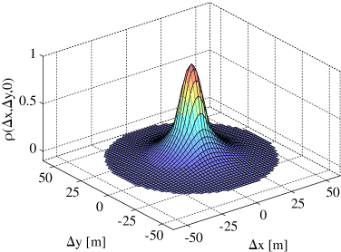
In the following, we present numerical results for the proposed estimation method. To demonstrate the approximation of an arbitrary ACFs, we study the performance of the model for a combination of a Gaussian and an exponential ACF which has the same decorrelation distance as (2) with closely spaced samples showing a higher correlation.

$$\rho(d)=\left\{\begin{array}[]{ll}\exp\left(-\frac{d^{2}}{d_{\lambda}^{2}}\right),&\hbox{for $d<d_{\lambda}$;}\\ \exp\left(-\frac{d}{d_{\lambda}}\right),&\hbox{for $d\geq d_{\lambda}$}\end{array}\right.$$ (22)

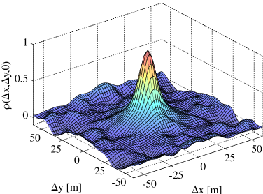
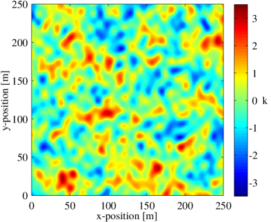
Results for the exponential ACF are presented at the end of this section. The decorrelation distance $d_{\lambda}$ was set to 10 meters and the ACF was sampled in intervals of 0.25 meters ranging from 0 to 49.75 meters. Hence, $\rho(d_{s})$ contains 200 values. A 2-D plot of this function is shown in Fig. 1 (top). This function was approximated using the method outlined in section III with a varying number of sinusoid coefficients. The number of test directions for the iterative search was set to 28 and the entire estimation process was repeated 5000 times with different initial values for the directions $(\theta_{n},\phi_{n})$ and the initial root-frequencies. Fig. 1 (bottom) shows the best result of an approximation using 300 sinusoids. An example of the 2-D random process resulting from this approximation is shown in Fig. 2. The output was generated by defining $x,y$-positions on a 250 $\times$ 250 m grid with 0.5 m spacing. The $z$-position was set to 0 m and no D2D extension was used.

Figure 1: Desired 2-D ACF on the $x-y$ plane (top) and approximated ACF using 300 sinusoids (bottom)

Figure 2: Example of a spatially correlated 2-D process

ACF approximation accuracy

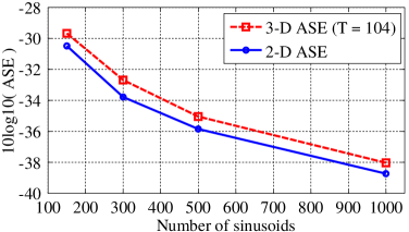
The achievable ASE as a function of the number of sinusoids is shown in Figure 3 (lower values are better). The red dashed curve shows the ASE calculation using (16) whereas the blue, solid line compares the 2-D ACFs on the $x-y$, $x-z$, and $y-z$ plane with the one shown in Fig. 1 (taking only the disk-shaped area covered by the ACF into account). Both methods estimate similar values for the ASE. The curves indicate that when doubling the number of coefficients, the ASE improves by roughly 3 dB. However, this also comes at the cost of doubling the computation time for the generation of the random numbers.

Figure 3: Achievable ASE vs. number of sinusoids for the combined ACF

Random number generation

Figure 4: Estimated ACF from spatially correlated random values

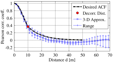
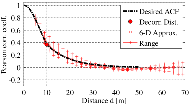
Figure 4 compares the desired ACF (thick dashed line) with the output of the random number generator using 300 sinusoids. For the upper plot, 6000 positions were randomly chosen within a cube of 56 m edge length. Then, spatially correlated Normal distributed random numbers were generated for each position using (4). The distance between each pair of positions was calculated and pairs with similar distance were grouped, i.e. positions with a distance between 0 and 2 meters of each other belong to group 1, positions with a distance between 2 and 4 meters belong to group 2, and so on. The Pearson correlation coefficient was calculated for the samples within each group. The entire process was repeated 10 times to obtain an average ACF (blue squares) and the spread for different initializations (bars showing the minimum and maximum values of the 10 initializations). For the lower part of the figure, 3000 positions were randomly chosen for the transmitter and 3000 were chosen for the receiver. Then, spatially correlated values were generated using (19). The grouping was done for the transmitter positions under the constraint that the receiver does not move faster than the transmitter. For example, group 3 contains all pairs where the transmitters have a distance between 4 and 6 meters and the receivers have a distance between 0 and 6 meters of each other. Both curves indicate that the given ACF can be approximated with good accuracy.

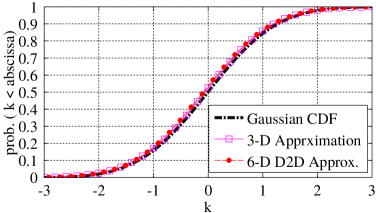
Figure 5 shows that the CDF of the generated random numbers is close to Gaussian density. For this, $10^{4}$ random positions were generated in a cube of $1000\times 1000\times 50$ m edge length and spatially correlated random numbers were generated using (4) and (19). There is no notable difference between the distribution of the generated values and the Gaussian CDF.

Figure 5: CDF of the output values vs. the Gaussian CDF

Complexity considerations

As mentioned in the introduction, the state-of-the-art alternative for the generation of correlated random numbers is by filtering white noise [5]. Here, the filter approach is compared with the SOS model in terms of memory requirements, initialization time, time to generate the output values, and the restrictions on the MT placement. The results are summarized in Table I.

TABLE I: Performance comparison of filter-based and SOS model

	Filter approach	Sum-of-sinusoids
Required memory	$N^{D}$ elements	$(D+1)\cdot N$ elements
Initialization	$\approx D\cdot S\cdot N^{D}$ op.	$\approx N$ operations
Output generation	$2D^{2}+5D$ op.	$\approx N\cdot(2D+15)$ op.
MT placement	inside map area	no restriction

For the filter approach, the parameter $N$ in Tab. I refers to the edge length of the sampled area and $D$ refers to the number of dimensions. The sample resolution needs to be high enough to captures the variation in the random process. With $d_{\lambda}=10$ m, we assume that a resolution of 2.5 m is sufficient. With $N=300$ and $D=2$, the filtered map covers an area of $750\times 750$ meters and requires 360 kilobytes of memory. Without increasing $N$ or lowering the resolution, all MTs must be located within this area. In comparison, the SOS method requires only 3.6 kilobytes of memory for the sinusoid coefficients and there are no restrictions on the MT positions.

Initializing the random number generator means that a new map must be generated, i.e. for the filter approach, generating $N^{D}$ random numbers and processing each number with $D$ finite impulse response filters of order $S$. For the SOS method, only the $N$ phases $\psi_{n}$ must be randomly initialized in (4). The sinusoid frequencies can be precalculated and stored in a table. This makes the SOS method very efficient when many random variables are needed, such as for the spacial consistency model from 3GPP [1]. The downside of the SOS method resides in the commutation time required to generate the correlated output values. Calculating the cosine in (4) is computationally expensive and the sum over all $N$ sinusoids must be calculated for each output value. With $N=300$ and $D=2$, approximately 5700 operations are needed to generate one output value. For the filter approach, the map only needs to be interpolated to obtain the output value at the MT position. This requires 18 operations using bilinear interpolation. Hence, the filter approach might be preferred when the output value generation is the dominating factor in the overall computing time.

Exponential ACF approximation

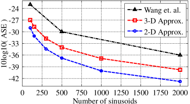
The achievable ASE performance is compared with the results from Wang et. al. [9], where an exponential ACF was approximated by different methods using 100, 500, and 2000 sinusoids. With the Monte Carlo method, [9] reported an ASE for a 2-D approximation of $-23$ dB, $-30$ dB, and $-36$ dB, respectively. The other proposed methods performed similarly. Our iterative approximation method achieved $-29$ dB, $-36.8$ dB, and $-42.7$ dB for the 2-D approximation of the exponential ACF using the same number of sinusoids, respectively. This is an average improvement of $6.5$ dB. Results are shown in Fig. 6. The 3-D approximation has an average performance loss of 2.7 dB compared to 2-D . However, this is still a significant improvement compared to [9].

Figure 6: Achievable ASE vs. number of sinusoids for the exponential ACF

VI Conclusions

The proposed iterative approximation method can obtain the sinusoid coefficients for arbitrary autocorrelation functions with better accuracy compared to previous results. It is possible to change the decorrelation distance and the distribution of the spatially correlated random process without recalculating the sinusoid frequencies. They can be precomputed and stored in a table for fast access. Therefore, generating spatially correlated random numbers, even for a large number of positions, can be done by simply calculating a weighted sum. The performance scales linearly with the number of sinusoids and the number of positions. Furthermore, memory requirements are negligible. This provides a very efficient implementation of the 3GPP proposal for spatial consistency. The scheme can be used with minimal adjustments to support a system where both ends of a link are mobile.

References

- [1] 3GPP TR 38.901 v14.1.0, “Study on channel model for frequencies from 0.5 to 100 GHz,” Tech. Rep., 2017.
- [2] S. Jaeckel, “Quasi-deterministic channel modeling and experimental validation in cooperative and massive mimo deployment topologies,” Ph.D. dissertation, TU Ilmenau, 2017. [Online]. Available: https://www.db-thueringen.de
- [3] [Online]. Available: http://www.quadriga-channel-model.de
- [4] M. Narandzic, M. Käske, S. Jäckel, G. Sommerkorn, C. Schneider, and R. S. Thomä, “Variation of estimated large-scale MIMO channel properties between repeated measurements,” Proc. IEEE VTC ’11 Spring, 2011.
- [5] K. Bakowski and K. Wesolowski, “Change the channel,” IEEE Veh. Technol. Mag., vol. 6, pp. 82–91, 2011.
- [6] T. Jamsa and P. Kyosti, “Device-to-device extension to geometry-based stochastic channel models,” Antennas and Propagation (EuCAP), 2015 9th European Conference on, pp. 1–4, April 2015.
- [7] M. Patzold, U. Killat, and F. Laue, “A deterministic digital simulation model for suzuki processes with application to a shadowed rayleigh land mobile radio channel,” IEEE Transactions on Vehicular Technology, vol. 45, no. 2, pp. 318–331, May 1996.
- [8] X. Cai and G. B. Giannakis, “A two-dimensional channel simulation model for shadowing processes,” IEEE Trans. Veh. Technol., vol. 52, no. 6, pp. 1558–1567, 2003.
- [9] Z. Wang, E. Tameh, and A. Nix, “A sum-of-sinusoids based simulation model for the joint shadowing process in urban peer-to-peer radio channels,” Proc. IEEE VTC ’05 Fall, vol. 3, pp. 1732–1736, Sept 2005.
- [10] M. Gudmundson, “Correlation model for shadow fading in mobile radio systems,” IET Electron Lett., vol. 27, no. 23, pp. 2145–2146, November 1991.
- [11] M. Deserno, “How to generate equidistributed points on the surface of a sphere,” Max-Planck-Institut für Polymerforschung, Tech. Rep., 2004.
- [12] P. Hoeher, “A statistical discrete-time model for the wssus multipath channel,” IEEE Transactions on Vehicular Technology, vol. 41, no. 4, pp. 461–468, 1992.