11institutetext: Quoc Tran-Dinh 22institutetext: Department of Statistics and Operations Research, University of North Carolina at Chapel Hill (UNC-Chapel Hill), 333 Hanes Hall, CB#3260, UNC Chapel Hill, NC 27599-3260.
22email: quoctd@email.unc.edu
33institutetext: Ahmet Alacaoglu 44institutetext: Volkan Cevher 55institutetext: Laboratory for Information and Inference Systems (LIONS), École Polytechnique Fédérale de Lausanne (EPFL), CH1015-Lausanne, Switzerland.
55email: {ahmet.alacaoglu, volkan.cevher}@epfl.ch
66institutetext: Olivier Fercoq 77institutetext: LTCI, Télécom ParisTech, Université Paris-Saclay, 75634-Paris, France.
77email: olivier.fercoq@telecom-paristech.fr

An Adaptive Primal-Dual Framework for
Nonsmooth Convex Minimization

Quoc Tran-Dinh    Ahmet Alacaoglu    Olivier Fercoq    Volkan Cevher
(Received: date / Accepted: date)
Abstract

We propose a new self-adaptive, double-loop smoothing algorithm to solve composite, nonsmooth, and constrained convex optimization problems. Our algorithm is based on Nesterov’s smoothing technique via general Bregman distance functions. It self-adaptively selects the number of iterations in the inner loop to achieve a desired complexity bound without requiring the accuracy a priori as in variants of Augmented Lagrangian methods (ALM). We prove 𝒪(1k)𝒪1𝑘\mathcal{O}\left(\frac{1}{k}\right)-convergence rate on the last iterate of the outer sequence for both unconstrained and constrained settings in contrast to ergodic rates which are common in ALM as well as alternating direction method-of-multipliers literature. Compared to existing inexact ALM or quadratic penalty methods, our analysis does not rely on the worst-case bounds of the subproblem solved by the inner loop. Therefore, our algorithm can be viewed as a restarting technique applied to the ASGARD method in TranDinh2015b but with rigorous theoretical guarantees or as an inexact ALM with explicit inner loop termination rules and adaptive parameters. Our algorithm only requires to initialize the parameters once, and automatically update them during the iteration process without tuning. We illustrate the superiority of our methods via several examples as compared to the state-of-the-art.

Keywords:
primal-dual first-order methods restarting augmented Lagrangian homotopy nonsmooth convex optimization constrained convex programming
MSC:
90C25 90C06 90-08

1 Introduction

We study the following nonsmooth composite convex minimization template:

P:=minxp{P(x):=f(x)+g(Ax)},assignsuperscript𝑃subscript𝑥superscript𝑝assign𝑃𝑥𝑓𝑥𝑔𝐴𝑥P^{\star}:=\min_{x\in\mathbb{R}^{p}}\Big{\{}P(x):=f(x)+g(Ax)\Big{\}}, (1)

where both f:p{+}:𝑓superscript𝑝f:\mathbb{R}^{p}\to\mathbb{R}\cup\{+\infty\} and g:n{+}:𝑔superscript𝑛g:\mathbb{R}^{n}\to\mathbb{R}\cup\{+\infty\} are proper, closed, and nonsmooth convex functions, and A:pn:𝐴superscript𝑝superscript𝑛A:\mathbb{R}^{p}\rightarrow\mathbb{R}^{n} is a linear operator.

Under only convexity and zero duality gap assumptions, the state-of-the-art methods for solving (1) include primal-dual first-order methods (PDFOM) Bauschke2011 ; Chambolle2011 , and augmented Lagrangian-based algorithms Bertsekas1996d ; Boyd2011 . While PDFOM directly tackles problem (1), the augmented Lagrangian-based framework (ALM) and its variants solve (1) via a constrained reformulation as follows:

P:=minxp,zn{P(x,z):=f(x)+g(z)s.t.Axz=0},P^{\star}:=\min_{x\in\mathbb{R}^{p},z\in\mathbb{R}^{n}}\Big{\{}P(x,z):=f(x)+g(z)~{}~{}\mathrm{s.t.}~{}~{}Ax-z=0\Big{\}}, (2)

Alternating direction method of multipliers (ADMM) is another (and perhaps the most) successful method to solve (2). ADMM can be viewed as an approximation to ALM by alternating between x𝑥x and z𝑧z to break the computational bottleneck in the primal subproblem. Inexact and linearized variants enhance the scalability of ALM and ADMM for the same problem template xu2017accelerated ; ouyang2015accelerated ; xu2017iteration .

While ADMM and PDFOM and their variants work really well in practice, their best-known convergence rate is 𝒪(1k)𝒪1𝑘\mathcal{O}\left(\frac{1}{k}\right) under only convexity and zero duality gap assumptions, where k𝑘k is the iteration counter. Moreover, such a rate is achieved via an ergodic sense (i.e., using an averaging sequence or a weighted averaging sequence) Chambolle2011 ; chambolle2016ergodic ; Davis2014b ; Davis2014 ; Monteiro2010 ; Monteiro2012b ; Shefi2014 .

In stark contrast, empirical evidence shows that averaging sequences in PDFOM and ALM exhibit the theoretical worst case rate 𝒪(1k)𝒪1𝑘\mathcal{O}\left(\frac{1}{k}\right) in practice compared to the last iterate of the algorithm (see Subsection 4.1 for a concrete example), which is superior and often locally linear in many examples.111There exist examples showing arbitrarily slow convergence rate of ADMM, see, e.g., Davis2014b . However, for these methods, last iterate generally has convergence guarantees but has no rate guarantees.

Recently, TranDinh2015b proposed an accelerated, smoothed gap reduction (ASGARD) framework to solve nonsmooth convex optimization problems. ASGARD combines acceleration, smoothing, and homotopy techniques to handle both unconstrained and constrained nonsmooth problems, including (1).

One notable feature of ASGARD is a non-ergodic optimal 𝒪(1k)𝒪1𝑘\mathcal{O}\left(\frac{1}{k}\right) rate on the objective residual, and feasibility violation in the constrained settings. Moreover, this method only requires one proximal operator of f𝑓f, one matrix-vector multiplication, and one adjoint operator per iteration. When f𝑓f is separable, the algorithm can be naturally parallelized. However, as also noted in TranDinh2015b , ASGARD needs restarting to be competitive with state-of-the-art methods such as ADMM and PDFOM in practice. This is not surprising since empirical evidence fercoq2016restarting ; Giselsson2014 ; Odonoghue2012 ; Su2014 has shown that restarting significantly improves the actual convergence rate in practice. While there exists theory to support the restarting strategies in accelerated gradient-type methods, supporting theory of these strategies are not yet investigated in primal-dual methods.

In this paper, we introduce an analysis framework for restarting ASGARD and prove the same worst-case 𝒪(1k)𝒪1𝑘\mathcal{O}\left(\frac{1}{k}\right) rate in a non-ergodic sense. To our knowledge, this is the first time restarting is studied for primal-dual methods with a rigorous convergence rate guarantee. While doing so, we identify that restarting ASGARD corresponds to an inexact ALM algorithm in the constrained case. In contrast to existing works on this front, our method has explicit inner-loop termination rules and does not need to set a horizon (i.e., the maximum number of inner iterations or a predefined inner loop accuracy) for the algorithm.

As a result, we present a method which has the guarantees on the last iterate compared to ALM/ADMM methods and extend the guarantees of ASGARD to the restarting case which significantly improves the practical performance. In addition, we allow general Bregman distances to be used for smoothing and proximal operators in contrast to the original ASGARD scheme. A more thorough discussion and comparison between our method and existing state-of-the-arts is deferred to Section 5 for the sake of presentation.

Composite vs. constrained settings:

An interesting instance of (1) is the following constrained convex setting:

f:=minxp{f(x)Axb𝒦},assignsuperscript𝑓subscript𝑥superscript𝑝conditional𝑓𝑥𝐴𝑥𝑏𝒦f^{\star}:=\min_{x\in\mathbb{R}^{p}}\Big{\{}f(x)~{}\mid~{}Ax-b\in\mathcal{K}\Big{\}}, (3)

where 𝒦𝒦\mathcal{K} is a nonempty, closed, and convex set in nsuperscript𝑛\mathbb{R}^{n}, and bn𝑏superscript𝑛b\in\mathbb{R}^{n}. If we define g(u):=δb+𝒦(u)assign𝑔𝑢subscript𝛿𝑏𝒦𝑢g(u):=\delta_{b+\mathcal{K}}(u), the indicator of b+𝒦𝑏𝒦b+\mathcal{K}, then (3) can be converted into (1).

In the general setting (1), under different choices of f𝑓f and g𝑔g, (1) covers a wide range of applications from different fields including compressive sensing, image/signal processing, machine learning, statistics, and optimal control. Classical and well-known examples such as LASSO, square-root LASSO, support vector machines, image denoising and deblurring, and matrix completion can be cast into (1), see, e.g., Boyd2011 ; Combettes2011 ; Parikh2013 ; wright2017optimization for some concrete examples.

For the setting (3), we do not impose any restriction on 𝒦𝒦\mathcal{K}. Hence, it covers a large class of constrained problems including equality and inequality constraints. When 𝒦𝒦\mathcal{K} is a given cone (e.g., +nsubscriptsuperscript𝑛\mathbb{R}^{n}_{+}, second-order cone, or symmetric positive semidefinite cone), problem (3) covers also problems with cone constraints such as linear programming, second-order cone, and semidefinite programming. Although the theory for (1) as well as for (3) are well developed, various numerical methods for solving these problems rely on different structure assumptions and do not have a unified analysis: cf., Section 5.

Contributions:

Our contributions can be summarized as follows.

  • (a)a\mathrm{(a)}

    We propose a new self-adaptive, double-loop smoothing algorithm to solve nonsmooth convex optimization problems of the form (1). Our algorithm is based on Nesterov’s smoothing technique via general Bregman distance functions. It self-adaptively selects the number of iterations in the inner loop to achieve a desired complexity bound without requiring the accuracy a priori as in variants of ALM. Compared to ASGARD TranDinh2015b , it incorporates restarts, updates the dual center, and can work with general Bregman distances instead of only Lipschitz gradient distances.

  • (b)b\mathrm{(b)}

    We prove 𝒪(1k)𝒪1𝑘\mathcal{O}\left(\frac{1}{k}\right)-convergence rate on the last iterate of the outer sequence for both unconstrained and constrained settings in contrast to ergodic rates which are common in ALM/ADMM literature. This rate is known to be optimal Nemirovskii1983 ; Nesterov2005c ; woodworth2016tight under just convexity and strong duality assumptions. Compared to existing inexact ALM or quadratic penalty methods such as necoara2015complexity ; xu2016homotopy , our analysis does not rely on the worst-case bounds of the subproblem solved by the inner loop. Therefore, our algorithm can be viewed as a restarting technique applied to ASGARD but with rigorous theoretical guarantees or as an inexact ALM with explicit inner loop termination rules and adaptive parameters.

  • (c)c\mathrm{(c)}

    As an upshot, we customize our algorithm to solve general constrained problems of the form (3). We prove the same 𝒪(1k)𝒪1𝑘\mathcal{O}\left(\frac{1}{k}\right)-convergence rate guarantee on both the objective residual |f(xk)f(x)|𝑓superscript𝑥𝑘𝑓superscript𝑥|f(x^{k})-f(x^{\star})| and the feasibility dist𝒦(Axkb)subscriptdist𝒦𝐴superscript𝑥𝑘𝑏\mathrm{dist}_{\mathcal{K}}\left(Ax^{k}-b\right). This rate is given on the last iterate of the outer sequence.

Our algorithm is a primal-dual method, which can solve composite convex problem with linear operators as in Chambolle-Pock’s method Chambolle2011 . It only requires one proximal operator of f𝑓f and gsuperscript𝑔g^{*}, one matrix-vector multiplication and one adjoint for each iteration. It is parallelizable when f𝑓f is separable, i.e., f(x)=i=1Nfi(x[i])𝑓𝑥superscriptsubscript𝑖1𝑁subscript𝑓𝑖subscript𝑥delimited-[]𝑖f(x)=\sum_{i=1}^{N}f_{i}(x_{[i]}). Under this structure, our method has more advantages than ADMM and Chambolle-Pock’s method. In the algorithm, we provide explicit rules to update all algorithmic parameters. We also note that these updates can be modified to trade-off between the primal or the dual progress.

Paper organization:

The rest of this paper is organized as follows. Section 2 recalls some mathematical background and the ASGARD algorithm in TranDinh2015b . Section 3 presents our main result with algorithm and its convergence guarantee. We study both unconstrained and constrained cases. Section 3.3 shows an extension of our method to three composite objective functions with linearization on potentially smooth terms. We provide overall complexity bounds in Section 3.4 for linear programming and discuss their superiority compared to existing results. In Section 4, we provide seven numerical examples to test our algorithm against state-of-the arts. Section 5 compares our method and existing algorithms in the literature.

2 Mathematical tools and ASGARD

We review some key ingredients for the design of our primal-dual methods. We also recall the ASGARD algorithm in TranDinh2015b and discuss its possible variants.

Notation:

We denote the norm in primal space 𝒳𝒳\mathcal{X} as 𝒳\|\cdot\|_{\mathcal{X}} and the norm in dual space 𝒴𝒴\mathcal{Y} as 𝒴\|\cdot\|_{\mathcal{Y}}. Their dual norms are denoted as 𝒳,\|\cdot\|_{\mathcal{X},\ast} and 𝒴,\|\cdot\|_{\mathcal{Y},\ast}, respectively. Given a proper, closed, and convex function f𝑓f, we use dom(f)dom𝑓\mathrm{dom}(f) to denote its domain and f(x)𝑓𝑥\partial f(x) to denote its subdifferential at x𝑥x. When the function is differentiable, we denote its gradient at x𝑥x as f(x)𝑓𝑥\nabla f(x). For a given nonempty, closed, and convex set 𝒦𝒦\mathcal{K}, we denote its indicator function as δ𝒦(x)=0subscript𝛿𝒦𝑥0\delta_{\mathcal{K}}(x)=0, if x𝒦𝑥𝒦x\in\mathcal{K}, δ𝒦(x)=+subscript𝛿𝒦𝑥\delta_{\mathcal{K}}(x)=+\infty, otherwise; and its support function as s𝒦(y)=supx𝒦x,ysubscript𝑠𝒦𝑦subscriptsupremum𝑥𝒦𝑥𝑦s_{\mathcal{K}}(y)=\sup_{x\in\mathcal{K}}\langle x,y\rangle. We define the normal cone of 𝒦𝒦\mathcal{K} as 𝒩𝒦(x):={wnw,yx0,y𝒦}assignsubscript𝒩𝒦𝑥conditional-set𝑤superscript𝑛formulae-sequence𝑤𝑦𝑥0𝑦𝒦\mathcal{N}_{\mathcal{K}}(x):=\left\{w\in\mathbb{R}^{n}\mid\langle w,y-x\rangle\geq 0,~{}y\in\mathcal{K}\right\} if x𝒦𝑥𝒦x\in\mathcal{K}; 𝒩𝒦(x):=assignsubscript𝒩𝒦𝑥\mathcal{N}_{\mathcal{K}}(x):=\emptyset, otherwise. We also define 𝒦o:={wnw,x1,x𝒦}assignsuperscript𝒦𝑜conditional-set𝑤superscript𝑛formulae-sequence𝑤𝑥1𝑥𝒦\mathcal{K}^{o}:=\left\{w\in\mathbb{R}^{n}\mid\langle w,x\rangle\leq 1,~{}x\in\mathcal{K}\right\} as the polar set of 𝒦𝒦\mathcal{K}. If 𝒦𝒦\mathcal{K} is a convex cone, then 𝒦o=𝒦superscript𝒦𝑜superscript𝒦\mathcal{K}^{o}=-\mathcal{K}^{\ast}, where 𝒦:={wnw,x0,x𝒦}assignsuperscript𝒦conditional-set𝑤superscript𝑛formulae-sequence𝑤𝑥0𝑥𝒦\mathcal{K}^{\ast}:=\left\{w\in\mathbb{R}^{n}\mid\langle w,x\rangle\geq 0,~{}x\in\mathcal{K}\right\} the dual cone of 𝒦𝒦\mathcal{K}. The Fenchel conjugate of a function f𝑓f is defined as f(y):=supx{x,yf(x)}assignsuperscript𝑓𝑦subscriptsupremum𝑥𝑥𝑦𝑓𝑥f^{\ast}(y):=\sup_{x}\left\{\langle x,y\rangle-f(x)\right\}. We say that f:𝒳:𝑓𝒳f:\mathcal{X}\rightarrow\mathbb{R} has Lipschitz gradient if it satisfies f(x)f(y)𝒳,Lfxy𝒳subscriptnorm𝑓𝑥𝑓𝑦𝒳subscript𝐿𝑓subscriptnorm𝑥𝑦𝒳\left\|\nabla f(x)-\nabla f(y)\right\|_{\mathcal{X},\ast}\leq L_{f}\left\|x-y\right\|_{\mathcal{X}}, for any x,y𝒳𝑥𝑦𝒳x,y\in\mathcal{X}. This is equivalent to f(x)f(y)+f(y),xy+Lf2xy𝒳2𝑓𝑥𝑓𝑦𝑓𝑦𝑥𝑦subscript𝐿𝑓2superscriptsubscriptnorm𝑥𝑦𝒳2f(x)\leq f(y)+\langle\nabla f(y),x-y\rangle+\tfrac{L_{f}}{2}\left\|x-y\right\|_{\mathcal{X}}^{2}, for all x,y𝒳𝑥𝑦𝒳x,y\in\mathcal{X}. Given a positive real number a𝑎a, a𝑎\lfloor a\rfloor denotes the largest integer that is less than or equal to a𝑎a.

Given a proper, closed, and convex function f:p{+}:𝑓superscript𝑝f:\mathbb{R}^{p}\to\mathbb{R}\cup\{+\infty\}, proxf(x):=argminu{f(u)+(1/2)ux𝒳2}assignsubscriptprox𝑓𝑥argsubscript𝑢𝑓𝑢12superscriptsubscriptnorm𝑢𝑥𝒳2\mathrm{prox}_{f}(x):=\mathrm{arg}\!\min_{u}\left\{f(u)+(1/2)\|u-x\|_{\mathcal{X}}^{2}\right\} is called the proximal operator of f𝑓f. We say that f𝑓f is “proximally tractable” if proxfsubscriptprox𝑓\mathrm{prox}_{f} can be computed efficiently, e.g., in a closed form, or by a polynomial algorithm. By Moreau’s identity, we have proxγf(x)+γproxf/γ(γ1x)=xsubscriptprox𝛾𝑓𝑥𝛾subscriptproxsuperscript𝑓𝛾superscript𝛾1𝑥𝑥\mathrm{prox}_{\gamma f}(x)+\gamma\mathrm{prox}_{f^{\ast}/\gamma}(\gamma^{-1}x)=x for any xdom(f)𝑥dom𝑓x\in\mathrm{dom}(f).

2.1 Primal-dual formulation

Dual problem and min-max formulation: Associated with the primal problem (1), we also consider the corresponding dual problem:

D:=minyn{D(y):=f(Ay)+g(y)},assignsuperscript𝐷subscript𝑦superscript𝑛assign𝐷𝑦superscript𝑓superscript𝐴top𝑦superscript𝑔𝑦D^{\star}:=\min_{y\in\mathbb{R}^{n}}\Big{\{}D(y):=f^{\ast}(-A^{\top}y)+g^{\ast}(y)\Big{\}}, (4)

where fsuperscript𝑓f^{\ast} and gsuperscript𝑔g^{\ast} are the Fenchel conjugates of f𝑓f and g𝑔g, respectively. Clearly, we can write the primal and dual pair (1)-(4) in the following min-max saddle point problem:

P=minxpmaxyn{f(x)+Ax,yg(y)}=maxynminxp{g(y)(x,Ayf(x))}=D.superscript𝑃absentsubscript𝑥superscript𝑝subscript𝑦superscript𝑛𝑓𝑥𝐴𝑥𝑦superscript𝑔𝑦missing-subexpressionabsentsubscript𝑦superscript𝑛subscript𝑥superscript𝑝superscript𝑔𝑦𝑥superscript𝐴top𝑦𝑓𝑥superscript𝐷\begin{array}[]{ll}P^{\star}&=\displaystyle\min_{x\in\mathbb{R}^{p}}\displaystyle\max_{y\in\mathbb{R}^{n}}\Big{\{}f(x)+\langle Ax,y\rangle-g^{\ast}(y)\Big{\}}\vspace{1ex}\\ &=\displaystyle\max_{y\in\mathbb{R}^{n}}\displaystyle\min_{x\in\mathbb{R}^{p}}\Big{\{}-g^{\ast}(y)-(\langle x,-A^{\top}y\rangle-f(x))\Big{\}}=-D^{\star}.\end{array} (5)

Under mild and standard assumptions, this min-max problem is solvable and achieves zero duality gap, i.e., P+D=0superscript𝑃superscript𝐷0P^{\star}+D^{\star}=0. In particular, the dual problem of (3) can be written as follows:

D:=minyn{D(y):=f(ATy)+b,y+s𝒦(y)},assignsuperscript𝐷subscript𝑦superscript𝑛assign𝐷𝑦superscript𝑓superscript𝐴𝑇𝑦𝑏𝑦subscript𝑠𝒦𝑦D^{\star}:=\min_{y\in\mathbb{R}^{n}}\left\{D(y):=f^{\ast}(-A^{T}y)+\langle b,y\rangle+s_{\mathcal{K}}(y)\right\}, (6)

where s𝒦(y)=supx𝒦y,xsubscript𝑠𝒦𝑦subscriptsupremum𝑥𝒦𝑦𝑥s_{\mathcal{K}}(y)=\sup_{x\in\mathcal{K}}\langle y,x\rangle is the support function of 𝒦𝒦\mathcal{K}. Compared to (4), we have g(y)=b,y+s𝒦(y)=sb+𝒦(y)superscript𝑔𝑦𝑏𝑦subscript𝑠𝒦𝑦subscript𝑠𝑏𝒦𝑦g^{\ast}(y)=\langle b,y\rangle+s_{\mathcal{K}}(y)=s_{b+\mathcal{K}}(y). Let 𝒳superscript𝒳\mathcal{X}^{\star} and 𝒴superscript𝒴\mathcal{Y}^{\star} be the solution sets of the primal problem (1) (or (3)) and dual problem (4) (or (6)), respectively.

Fundamental assumptions: Throughout this paper, we will develop methods for solving (1) and (3). Note that we will use different assumptions for these two cases, which are given below for  (1) and (3), respectively.

Assumption 2.1.

The solution set 𝒳superscript𝒳\mathcal{X}^{\star} of (1) is nonempty. Both f𝑓f and g𝑔g are proper, closed, and convex. Moreover, dom(g)domsuperscript𝑔\mathrm{dom}(g^{\ast}) is bounded, or equivalently, g𝑔g is Lipschitz continuous. Note that this implies the Slater condition 𝟎ri(dom(g)A(dom(f)))0ridom𝑔𝐴dom𝑓\boldsymbol{0}\in\mathrm{ri}\left(\mathrm{dom}(g)-A(\mathrm{dom}(f))\right), where ri(𝒳)ri𝒳\mathrm{ri}\left(\mathcal{X}\right) is the relative interior of 𝒳𝒳\mathcal{X}.

Assumption 2.2.

The solution set 𝒳superscript𝒳\mathcal{X}^{\star} of (3) is nonempty. The function f𝑓f is proper, closed, and convex. The constraint set 𝒦𝒦\mathcal{K} is nonempty, closed, and convex, and 𝟎n𝒦superscript0𝑛𝒦\boldsymbol{0}^{n}\in\mathcal{K}. The Slater condition ri(dom(f)){xpAxbri(𝒦)}ridom𝑓conditional-set𝑥superscript𝑝𝐴𝑥𝑏ri𝒦\mathrm{ri}\left(\mathrm{dom}(f)\right)\cap\left\{x\in\mathbb{R}^{p}\mid Ax-b\in\mathrm{ri}\left(\mathcal{K}\right)\right\}\neq\emptyset holds, where ri(𝒳)ri𝒳\mathrm{ri}\left(\mathcal{X}\right) is the relative interior of 𝒳𝒳\mathcal{X}.

Except for the boundedness of dom(g)domsuperscript𝑔\mathrm{dom}(g^{\ast}), Assumptions 2.1 and 2.2 are very standard in convex optimization. It guarantees the strong duality of (1) (respectively, (3)) and (4) to hold. The boundedness of dom(g)domsuperscript𝑔\mathrm{dom}(g^{\ast}) is guaranteed if and only if g𝑔g is Lipschitz continuous as we mentioned. We emphasize that we need boundedness of dom(g)domsuperscript𝑔\mathrm{dom}(g^{\ast}) only for (1) and we do not require it for (3)

We note that the assumption 𝟎n𝒦superscript0𝑛𝒦\boldsymbol{0}^{n}\in\mathcal{K} is not restrictive, since if 𝟎n𝒦superscript0𝑛𝒦\boldsymbol{0}^{n}\notin\mathcal{K}, we can fix any point 𝒆𝒦𝒆𝒦\boldsymbol{e}\in\mathcal{K}, and consider the set 𝒦~=𝒦𝒆~𝒦𝒦𝒆\tilde{\mathcal{K}}=\mathcal{K}-\boldsymbol{e}, then 𝟎n𝒦~superscript0𝑛~𝒦\boldsymbol{0}^{n}\in\tilde{\mathcal{K}}, and Axb𝒦𝐴𝑥𝑏𝒦Ax-b\in\mathcal{K} becomes Axb+𝒆𝒦~𝐴𝑥𝑏𝒆~𝒦Ax-b+\boldsymbol{e}\in\tilde{\mathcal{K}}. Note that, in the sequel, we will refer to the setting of (1) with Assumption 2.1 as the bounded dual domain case, and to the setting of (3) with Assumptions 2.2 as the constrained case.

Optimality conditions: Associated with the primal and dual problems (1)-(4), we have the following optimality conditions:

0f(x)+Ag(Ax)and0Af(Ay)+g(y).0𝑓superscript𝑥superscript𝐴top𝑔𝐴superscript𝑥and0𝐴superscript𝑓superscript𝐴topsuperscript𝑦superscript𝑔superscript𝑦0\in\partial{f}(x^{\star})+A^{\top}\partial{g}(Ax^{\star})~{}~{}~{}\text{and}~{}~{}~{}0\in-A\partial{f^{\ast}}(-A^{\top}y^{\star})+\partial{g^{\ast}}(y^{\star}). (7)

From (5), it is straightforward to see the relation yg(Ax)Axg(y)superscript𝑦𝑔𝐴superscript𝑥𝐴superscript𝑥superscript𝑔superscript𝑦y^{\star}\in\partial{g}(Ax^{\star})\Leftrightarrow Ax^{\star}\in\partial{g^{\ast}}(y^{\star}) and xf(Ay)Ayf(x)superscript𝑥superscript𝑓superscript𝐴topsuperscript𝑦superscript𝐴topsuperscript𝑦𝑓superscript𝑥x^{\star}\in\partial{f^{\ast}}(-A^{\top}y^{\star})\Leftrightarrow-A^{\top}y^{\star}\in\partial{f}(x^{\star}), we can write this optimality condition into the following KKT condition:

0f(x)+Ayand0Ax+g(y).0𝑓superscript𝑥superscript𝐴topsuperscript𝑦and0𝐴superscript𝑥superscript𝑔superscript𝑦0\in\partial{f}(x^{\star})+A^{\top}y^{\star}~{}~{}~{}\text{and}~{}~{}~{}0\in-Ax^{\star}+\partial{g^{\ast}}(y^{\star}).

For the constrained problem (3) these conditions are written as

0f(x)+Ay,Axb𝒦,andy𝒩𝒦(Axb),formulae-sequence0𝑓superscript𝑥superscript𝐴topsuperscript𝑦formulae-sequence𝐴superscript𝑥𝑏𝒦andsuperscript𝑦subscript𝒩𝒦𝐴superscript𝑥𝑏0\in\partial{f}(x^{\star})+A^{\top}y^{\star},~{}~{}~{}Ax^{\star}-b\in\mathcal{K},~{}~{}\text{and}~{}~{}y^{\star}\in\mathcal{N}_{\mathcal{K}}\left(Ax^{\star}-b\right),

where 𝒩𝒦()subscript𝒩𝒦\mathcal{N}_{\mathcal{K}}(\cdot) is the normal cone of 𝒦𝒦\mathcal{K} defined above. If 𝒦𝒦\mathcal{K} is a closed, pointed, and convex cone, then 𝒩𝒦𝒦subscript𝒩𝒦superscript𝒦\mathcal{N}_{\mathcal{K}}\equiv-\mathcal{K}^{\ast} the dual cone of 𝒦𝒦\mathcal{K}. In this case, y𝒦superscript𝑦superscript𝒦y^{\star}\in-\mathcal{K}^{\ast}.

2.2 Bregman Distances and Generalized Proximal Operators

In the sequel, we will use Bregman distances for smoothing and computing proximal operators. Therefore, we give basic properties on Bregman distances.

Let p𝒵subscript𝑝𝒵p_{\mathcal{Z}} be μpsubscript𝜇𝑝\mu_{p}-strongly convex, continuous, and differentiable on 𝒵𝒵\mathcal{Z} with the strong convexity μp=1subscript𝜇𝑝1\mu_{p}=1, where 𝒵=dom(p𝒵)𝒵domsubscript𝑝𝒵\mathcal{Z}=\text{dom}(p_{\mathcal{Z}}). We call p𝒵subscript𝑝𝒵p_{\mathcal{Z}} a proximity function (or prox-function). We define the Bregman distance induced by p𝒵subscript𝑝𝒵p_{\mathcal{Z}} as

b𝒵(x,y):=p𝒵(x)p𝒵(y)p𝒵(y),xy,x,y𝒵.formulae-sequenceassignsubscript𝑏𝒵𝑥𝑦subscript𝑝𝒵𝑥subscript𝑝𝒵𝑦subscript𝑝𝒵𝑦𝑥𝑦for-all𝑥𝑦𝒵b_{\mathcal{Z}}(x,y):=p_{\mathcal{Z}}(x)-p_{\mathcal{Z}}(y)-\langle\nabla p_{\mathcal{Z}}(y),x-y\rangle,~{}~{}\forall x,y\in\mathcal{Z}.

We assume that b𝒵subscript𝑏𝒵b_{\mathcal{Z}} is 111-strongly convex with respect to the norm 𝒵\|\cdot\|_{\mathcal{Z}}. Then

b𝒵(x,y)12xy𝒵2,x,y𝒵.formulae-sequencesubscript𝑏𝒵𝑥𝑦12superscriptsubscriptnorm𝑥𝑦𝒵2for-all𝑥𝑦𝒵b_{\mathcal{Z}}(x,y)\geq\tfrac{1}{2}\|x-y\|_{\mathcal{Z}}^{2},~{}~{}\forall x,y\in\mathcal{Z}. (8)

A special case of prox-functions is p𝒵(x)=12x22subscript𝑝𝒵𝑥12superscriptsubscriptnorm𝑥22p_{\mathcal{Z}}(x)=\frac{1}{2}\|x\|_{2}^{2}, which corresponds to the well-known Euclidean distance b𝒵(x,y)=12xy22subscript𝑏𝒵𝑥𝑦12superscriptsubscriptnorm𝑥𝑦22b_{\mathcal{Z}}(x,y)=\frac{1}{2}\|x-y\|_{2}^{2}. Another example is the entropy function p𝒵(x):=ixiln(xi)assignsubscript𝑝𝒵𝑥subscript𝑖subscript𝑥𝑖subscript𝑥𝑖p_{\mathcal{Z}}(x):=\sum_{i}x_{i}\ln(x_{i}), which corresponds to the so-called KL divergence b𝒵(x,y):=ixiln(xiyi)xi+yiassignsubscript𝑏𝒵𝑥𝑦subscript𝑖subscript𝑥𝑖subscript𝑥𝑖subscript𝑦𝑖subscript𝑥𝑖subscript𝑦𝑖b_{\mathcal{Z}}(x,y):=\sum_{i}x_{i}\ln\left(\frac{x_{i}}{y_{i}}\right)-x_{i}+y_{i}. When a Bregman distance b𝒵subscript𝑏𝒵b_{\mathcal{Z}} has Lipschitz continuous gradient, we denote its Lipschitz constant by Lb𝒵subscript𝐿subscript𝑏𝒵L_{b_{\mathcal{Z}}}.

We also define the strong convexity of a function f𝑓f with respect to a prox-function p𝒵subscript𝑝𝒵p_{\mathcal{Z}} which induces the Bregman distance b𝒵subscript𝑏𝒵b_{\mathcal{Z}} as follows:

f(x)f(y)+f(y),xy+b𝒵(x,y),x,y𝒵.formulae-sequence𝑓𝑥𝑓𝑦𝑓𝑦𝑥𝑦subscript𝑏𝒵𝑥𝑦for-all𝑥𝑦𝒵f(x)\geq f(y)+\langle\nabla f(y),x-y\rangle+b_{\mathcal{Z}}(x,y),~{}~{}~{}\forall x,y\in\mathcal{Z}. (9)

We refer to chen1993convergence ; eckstein1993nonlinear ; kiwiel1997proximal for several concrete examples of Bregman divergences.

2.3 Nesterov’s smoothing technique

We focus on Nesterov’s smoothing technique with general Bregman distances Beck2012a ; Nesterov2005c . Since g𝑔g is nonsmooth, assuming that it admits a max-form as

g(u)=maxy𝒴{u,yg(y)},where𝒴=dom(g),formulae-sequence𝑔𝑢subscript𝑦𝒴𝑢𝑦superscript𝑔𝑦where𝒴domsuperscript𝑔g(u)=\max_{y\in\mathcal{Y}}\left\{\langle u,y\rangle-g^{\ast}(y)\right\},~{}~{}~{}\text{where}~{}\mathcal{Y}=\mathrm{dom}(g^{\ast}),

we smooth it by

gβ(u;y˙):=maxy𝒴{u,yg(y)βb𝒴(y,y˙)},subscript𝑔𝛽𝑢˙𝑦assignabsentsubscript𝑦𝒴𝑢𝑦superscript𝑔𝑦𝛽subscript𝑏𝒴𝑦˙𝑦\begin{array}[]{ll}g_{\beta}(u;\dot{y})&:=\displaystyle\max_{y\in\mathcal{Y}}\left\{\langle u,y\rangle-g^{\ast}(y)-\beta b_{\mathcal{Y}}(y,\dot{y})\right\},\end{array} (10)

where y˙n˙𝑦superscript𝑛\dot{y}\in\mathbb{R}^{n} is a given center point, and β>0𝛽0\beta>0 is a smoothness parameter. The function gβ(;y˙)subscript𝑔𝛽˙𝑦g_{\beta}(\cdot;\dot{y}) is convex and smooth, its gradient is given by

gβ(u;y˙)=yβ(u;y˙)=argminy𝒴{g(y)u,y+βb𝒴(y,y˙)}.subscript𝑔𝛽𝑢˙𝑦subscriptsuperscript𝑦𝛽𝑢˙𝑦argsubscript𝑦𝒴superscript𝑔𝑦𝑢𝑦𝛽subscript𝑏𝒴𝑦˙𝑦\nabla{g_{\beta}}(u;\dot{y})=y^{\ast}_{\beta}(u;\dot{y})=\mathrm{arg}\!\min_{y\in\mathcal{Y}}\Big{\{}g^{\ast}(y)-\langle u,y\rangle+\beta b_{\mathcal{Y}}(y,\dot{y})\Big{\}}. (11)

Clearly, gβ(;y˙)subscript𝑔𝛽˙𝑦\nabla{g_{\beta}}(\cdot;\dot{y}) is Lipschitz continuous with the Lipschitz constant Lgβ=1βsubscript𝐿subscript𝑔𝛽1𝛽L_{g_{\beta}}=\frac{1}{\beta}. Moreover, we have

gβ(u;y˙)g(u)gβ(u;y˙)+βD𝒴,subscript𝑔𝛽𝑢˙𝑦𝑔𝑢subscript𝑔𝛽𝑢˙𝑦𝛽subscript𝐷𝒴g_{\beta}(u;\dot{y})\leq g(u)\leq g_{\beta}(u;\dot{y})+\beta D_{\mathcal{Y}}, (12)

where D𝒴:=sup{b𝒴(y,y˙)ydom(g)}assignsubscript𝐷𝒴supremumconditional-setsubscript𝑏𝒴𝑦˙𝑦𝑦domsuperscript𝑔D_{\mathcal{Y}}:=\sup\left\{b_{\mathcal{Y}}(y,\dot{y})\mid y\in\mathrm{dom}(g^{\ast})\right\} is the prox-diameter of gsuperscript𝑔g^{\ast}. Here, D𝒴subscript𝐷𝒴D_{\mathcal{Y}} is finite if and only if g𝑔g is Lipschitz continuous with the Lipschitz constant Lg:=2D𝒴assignsubscript𝐿𝑔2subscript𝐷𝒴L_{g}:=\sqrt{2D_{\mathcal{Y}}}, i.e., |g(u)g(v)|2D𝒴uv𝑔𝑢𝑔𝑣2subscript𝐷𝒴norm𝑢𝑣|g(u)-g(v)|\leq\sqrt{2D_{\mathcal{Y}}}\|u-v\| for all u,vdom(g)𝑢𝑣dom𝑔u,v\in\mathrm{dom}(g) due to (borwein2010convex, , Proposition 4.4.6).

If we choose b𝒴(y,y˙)=12yy˙22subscript𝑏𝒴𝑦˙𝑦12superscriptsubscriptnorm𝑦˙𝑦22b_{\mathcal{Y}}(y,\dot{y})=\frac{1}{2}\|y-\dot{y}\|_{2}^{2}, then we can write yβ(u;y˙)superscriptsubscript𝑦𝛽𝑢˙𝑦y_{\beta}^{\ast}(u;\dot{y}) as:

gβ(u;y˙)=argminyn{g(y)u,y+β2yy˙2}=proxg/β(y˙+1βu).subscript𝑔𝛽𝑢˙𝑦argsubscript𝑦superscript𝑛superscript𝑔𝑦𝑢𝑦𝛽2superscriptnorm𝑦˙𝑦2subscriptproxsuperscript𝑔𝛽˙𝑦1𝛽𝑢{\!\!\!\!}\nabla{g_{\beta}}(u;\dot{y})=\mathrm{arg}\!\min_{y\in\mathbb{R}^{n}}\left\{g^{\ast}(y)-\langle u,y\rangle+\tfrac{\beta}{2}\|y-\dot{y}\|^{2}\right\}=\mathrm{prox}_{g^{\ast}/\beta}\left(\dot{y}+\tfrac{1}{\beta}u\right).{\!\!\!\!} (13)

Smoothing techniques are widely used in the literature, including Beck2012a ; boct2012variable ; Bot2013 ; Devolder2012 ; Necoara2008 . The idea of smoothing is to approximate the original problem (1) by a (partially) smoothed problem. For example, in our setting, we smooth g𝑔g and consider the following smoothed problem:

Pβ:=minxp{Pβ(x;y˙):=f(x)+gβ(Ax;y˙)}.assignsuperscriptsubscript𝑃𝛽subscript𝑥superscript𝑝assignsubscript𝑃𝛽𝑥˙𝑦𝑓𝑥subscript𝑔𝛽𝐴𝑥˙𝑦P_{\beta}^{\star}:=\min_{x\in\mathbb{R}^{p}}\Big{\{}P_{\beta}(x;\dot{y}):=f(x)+g_{\beta}(Ax;\dot{y})\Big{\}}. (14)

We define the following generalized proximal operator with Bregman distance d𝒳subscript𝑑𝒳d_{\mathcal{X}} induced by a prox-function q𝒳subscript𝑞𝒳q_{\mathcal{X}}:

𝒫θfd𝒳(u,y):=argminv𝒳{f(v)+y,vu+1θd𝒳(v,u)}.assignsubscriptsuperscript𝒫subscript𝑑𝒳𝜃𝑓𝑢𝑦argsubscript𝑣𝒳𝑓𝑣𝑦𝑣𝑢1𝜃subscript𝑑𝒳𝑣𝑢\mathcal{P}^{d_{\mathcal{X}}}_{\theta f}(u,y):=\mathrm{arg}\!\min_{v\in\mathcal{X}}\Big{\{}f(v)+\langle y,v-u\rangle+\tfrac{1}{\theta}d_{\mathcal{X}}(v,u)\Big{\}}. (15)

Note that the setup described in this and previous subsections will allow us to use different Bregman distances for smoothing as in (10) and computing the proximal operator as in (15), depending on the geometry of the problem. Given that the Bregman distance d𝒳subscript𝑑𝒳d_{\mathcal{X}} is defined in 𝒳𝒳\mathcal{X} and b𝒴subscript𝑏𝒴b_{\mathcal{Y}} is defined in 𝒴𝒴\mathcal{Y}, we define the following operator norm of A𝐴A:

A:=maxxp{Ax𝒴,x𝒳}.assignnorm𝐴subscript𝑥superscript𝑝subscriptnorm𝐴𝑥𝒴subscriptnorm𝑥𝒳\left\|A\right\|:=\max_{x\in\mathbb{R}^{p}}\left\{\frac{\left\|Ax\right\|_{\mathcal{Y},\ast}}{\left\|x\right\|_{\mathcal{X}}}\right\}. (16)

Different from Beck2012a ; Bot2013 ; Devolder2012 ; Necoara2008 ; Nesterov2005c , our strategy allows one to update the smoothness parameter β𝛽\beta gradually at each iteration. Similar work can be found in boct2012variable ; Nesterov2005d , which are also essentially different from ours as discussed in Section 5.

2.4 ASGARD: A primal-dual gap reduction framework

In TranDinh2015b , the authors proposed two primal-dual algorithms to solve (1). The first algorithm, ASGARD (Accelerated Smoothed Gap Reduction), can be viewed as a variant of FISTA Beck2009 applied to the smoothed problem of (3). The second one, ADSGARD (Accelerated Dual Smoothed Gap Reduction) is a Nesterov’s accelerated variant Nesterov2004 applied to the smoothed problem of the dual (4).

ASGARD:

Let us recall the first algorithm, ASGARD, from TranDinh2015b as in Algorithm 1 for our further reference.

Algorithm 1 (ASGARDASGARD\mathrm{ASGARD} - Accelerated Smoothed GAp ReDuction)
1:Initialization:
2:Choose x0psuperscript𝑥0superscript𝑝x^{0}\in\mathbb{R}^{p}, y˙n˙𝑦superscript𝑛\dot{y}\in\mathbb{R}^{n}, and β0>0subscript𝛽00\beta_{0}>0 (e.g., β0:=Aassignsubscript𝛽0norm𝐴\beta_{0}:=\|A\|). Set τ01subscript𝜏01\tau_{0}\leftarrow 1 and x¯0=x^0x0superscript¯𝑥0superscript^𝑥0superscript𝑥0\bar{x}^{0}=\hat{x}^{0}\leftarrow x^{0}.
3:Choose d𝒳(,x˙)=12x˙2d_{\mathcal{X}}(\cdot,\dot{x})=\tfrac{1}{2}\|\cdot-\dot{x}\|^{2}, and a Bregman distance b𝒴subscript𝑏𝒴b_{\mathcal{Y}} as in Section 2.2.​​​
4:For k:=0assign𝑘0k:=0 to kmaxsubscript𝑘k_{\max} perform
5:      Update {x~k(1τk)x¯k+τkx^ky~k+1argminy𝒴{g(y)Ax~k,y+βkb𝒴(y,y˙)}x¯k+1𝒫(βk/A2)fd𝒳(x~k,Ay~k+1)x^k+1x^k+1τk(x¯k+1x~k).casessuperscript~𝑥𝑘absent1subscript𝜏𝑘superscript¯𝑥𝑘subscript𝜏𝑘superscript^𝑥𝑘superscript~𝑦𝑘1absentargsubscript𝑦𝒴superscript𝑔𝑦𝐴superscript~𝑥𝑘𝑦subscript𝛽𝑘subscript𝑏𝒴𝑦˙𝑦superscript¯𝑥𝑘1absentsubscriptsuperscript𝒫subscript𝑑𝒳subscript𝛽𝑘superscriptnorm𝐴2𝑓superscript~𝑥𝑘superscript𝐴topsuperscript~𝑦𝑘1superscript^𝑥𝑘1absentsuperscript^𝑥𝑘1subscript𝜏𝑘superscript¯𝑥𝑘1superscript~𝑥𝑘\left\{\begin{array}[]{ll}\tilde{x}^{k}&\leftarrow(1-\tau_{k})\bar{x}^{k}+\tau_{k}\hat{x}^{k}\vspace{0.75ex}\\ \tilde{y}^{k+1}&\leftarrow\displaystyle\mathrm{arg}\!\min_{y\in\mathcal{Y}}\left\{g^{\ast}(y)-\langle A\tilde{x}^{k},y\rangle+\beta_{k}b_{\mathcal{Y}}(y,\dot{y})\right\}\vspace{0.75ex}\\ \bar{x}^{k+1}&\leftarrow\mathcal{P}^{d_{\mathcal{X}}}_{(\beta_{k}/\left\|A\right\|^{2})f}\left(\tilde{x}^{k},A^{\top}\tilde{y}^{k+1}\right)\vspace{0.75ex}\\ \hat{x}^{k+1}&\leftarrow\hat{x}^{k}+\frac{1}{\tau_{k}}(\bar{x}^{k+1}-\tilde{x}^{k}).\end{array}\right.
6:      Compute τk+1(0,1)by solvingτ3Lb𝒴+τ2+τk2ττk2=0subscript𝜏𝑘101by solvingsuperscript𝜏3subscript𝐿subscript𝑏𝒴superscript𝜏2superscriptsubscript𝜏𝑘2𝜏superscriptsubscript𝜏𝑘20\tau_{k+1}\in(0,1)~{}\text{by solving}~{}\frac{\tau^{3}}{L_{b_{\mathcal{Y}}}}+\tau^{2}+\tau_{k}^{2}\tau-\tau_{k}^{2}=0 in τ𝜏\tau.
7:      Update βk+1βk1+Lb𝒴1τk+1subscript𝛽𝑘1subscript𝛽𝑘1superscriptsubscript𝐿subscript𝑏𝒴1subscript𝜏𝑘1\beta_{k+1}\leftarrow\frac{\beta_{k}}{1+L_{b_{\mathcal{Y}}}^{-1}\tau_{k+1}}.
8:End for

The main step of ASGARD, Algorithm 1, is Step 5, which requires one subproblem in y~k+1superscript~𝑦𝑘1\tilde{y}^{k+1}, one proxfsubscriptprox𝑓\mathrm{prox}_{f} of f𝑓f, one matrix-vector multiplication Ax𝐴𝑥Ax and its adjoint Aysuperscript𝐴top𝑦A^{\top}y at each iteration. If b𝒴(,y˙):=12y˙22b_{\mathcal{Y}}(\cdot,\dot{y}):=\tfrac{1}{2}\|\cdot-\dot{y}\|_{2}^{2}, then the computation of y~k+1superscript~𝑦𝑘1\tilde{y}^{k+1} reduces to proximal operator proxgsubscriptproxsuperscript𝑔\mathrm{prox}_{g^{\ast}} of gsuperscript𝑔g^{\ast}. Therefore, the per-iteration complexity of Algorithm 1 is the same as in several primal-dual first-order algorithms Chambolle2011 ; Esser2010a . In contrast to existing works, the convergence guarantee is on the last primal iterate {x¯k}superscript¯𝑥𝑘\left\{\bar{x}^{k}\right\}, instead of its weighted average {x~k}superscript~𝑥𝑘\left\{\tilde{x}^{k}\right\}.

Variants:

Although ASGARD relies on FISTA Beck2009 , one can replace Step 5 by any other accelerated proximal-gradient scheme such as Tseng’s variant (APG) in tseng2008accelerated . One can also use two proximal operator schemes from lan2011primal ; Nesterov2005c to substitute Step 5. To avoid the overload of this paper, we skip the analysis of Algorithm 1 and its variants, which can be found in TranDinh2015b .

Convergence:

As proved in TranDinh2015b , if Algorithm 1 is applied to solve (1) with b𝒴(;y˙):=12y˙𝒴2b_{\mathcal{Y}}(\cdot;\dot{y}):=\frac{1}{2}\|\cdot-\dot{y}\|_{\mathcal{Y}}^{2}, then, under Assumption 2.1, one has

P(x¯k)P𝒪(Ax0x𝒳D𝒴k).𝑃superscript¯𝑥𝑘superscript𝑃𝒪norm𝐴subscriptnormsuperscript𝑥0superscript𝑥𝒳subscript𝐷𝒴𝑘P(\bar{x}^{k})-P^{\star}\leq\mathcal{O}\left(\frac{\|A\|\|x^{0}-x^{\star}\|_{\mathcal{X}}D_{\mathcal{Y}}}{k}\right).

If we apply Algorithm 1 to solve the constrained problem (3), then, under Assumption 2.2, we obtain the following guarantee

{|f(x¯k)f|𝒪(Ax0x𝒳y𝒴k)dist𝒦(Ax¯kb)𝒪(Ax0x𝒳y𝒴k).casesmissing-subexpression𝑓superscript¯𝑥𝑘superscript𝑓absent𝒪norm𝐴subscriptnormsuperscript𝑥0superscript𝑥𝒳subscriptnormsuperscript𝑦𝒴𝑘missing-subexpressionsubscriptdist𝒦𝐴superscript¯𝑥𝑘𝑏absent𝒪norm𝐴subscriptnormsuperscript𝑥0superscript𝑥𝒳subscriptnormsuperscript𝑦𝒴𝑘\left\{\begin{array}[]{lll}&|f(\bar{x}^{k})-f^{\star}|&\leq\mathcal{O}\left(\dfrac{\|A\|\|x^{0}-x^{\star}\|_{\mathcal{X}}\|y^{\star}\|_{\mathcal{Y}}}{k}\right)\vspace{1ex}\\ &\mathrm{dist}_{\mathcal{K}}\left(A\bar{x}^{k}-b\right)&\leq\mathcal{O}\left(\dfrac{\|A\|\|x^{0}-x^{\star}\|_{\mathcal{X}}\|y^{\star}\|_{\mathcal{Y}}}{k}\right).\end{array}\right.

Hence, the convergence rate of Algorithm 1 under Assumption 2.1 or Assumption 2.2 is 𝒪(1k)𝒪1𝑘\mathcal{O}\left(\frac{1}{k}\right) and is in a non-ergodic sense.

3 Main results: Self-Adaptive Double-Loop ASGARD

In this section, we develop a self-adaptive double-loop accelerated smoothed primal-dual gap reduction algorithm to solve (1) and (3). We first present the complete algorithm. Next, we provide its convergence analysis. Then, we specify our algorithm to handle the constrained setting (3). Finally, we extend our method to handle (1) with the sum of three objective functions where the third function has Lipschitz gradient.

3.1 The algorithm and its convergence guarantee

Main idea: The proposed algorithm consists of two loops:

  • The inner loop performs an accelerated proximal gradient scheme (APG) tseng2008accelerated to solve the smoothed problem (14) for a fixed β𝛽\beta, which is a different strategy from TranDinh2015b , where β𝛽\beta is updated at each iteration. We note that in the constrained case, the smoothed problem (14) is the augmented Lagrangian.

  • The outer loop can be considered as a restarting step and simultaneously decreases the smoothness parameter β𝛽\beta.

The intuition behind our new strategy lies on the fact that when applied to (14) with a fixed β𝛽\beta, APG gets 𝒪(1k2)𝒪1superscript𝑘2\mathcal{O}\left(\frac{1}{k^{2}}\right) rate, whereas ASGARD as presented in TranDinh2015b controls the parameters in such a way that the algorithm gets 𝒪(1k)𝒪1𝑘\mathcal{O}\left(\frac{1}{k}\right) rate throughout its execution. The idea is to take the advantage of the faster rate of APG for the inner loop while carefully adjusting the number of inner iterations and the smoothness parameter to get the same overall 𝒪(1k)𝒪1𝑘\mathcal{O}\left(\frac{1}{k}\right) rate with better practical performance. Our analysis also gives insights on the heuristic restart strategy outlined in TranDinh2015b . For the sake of presentation and its flexibility for using Bregman distances in proximal operators, we choose Tseng’s variant of APG tseng2008accelerated . However, we can replace by another scheme such as FISTA Beck2009 . We adaptively determine the number of inner iterations at each outer iteration. Therefore, there is no need to tune this parameter. The outer loop gradually decreases the smoothness parameter β𝛽\beta such that the algorithm is still guaranteed to converge to the true solution of (1) or (3).

The algorithm: The complete algorithm is presented in Algorithm 2.

Algorithm 2 (Self-Adaptive Double Loop ASGARD Algorithm)
1:Initialization:
2:Choose β0>0subscript𝛽00\beta_{0}>0, ω>1𝜔1\omega>1, a positive integer m01subscript𝑚01m_{0}\geq 1, x¯0psuperscript¯𝑥0superscript𝑝\bar{x}^{0}\in\mathbb{R}^{p}, and y˙0nsuperscript˙𝑦0superscript𝑛\dot{y}^{0}\in\mathbb{R}^{n}.
3:Choose a Bregman distance b𝒴subscript𝑏𝒴b_{\mathcal{Y}} for y𝑦y and d𝒳subscript𝑑𝒳d_{\mathcal{X}} for x𝑥x.
4:Set K00subscript𝐾00K_{0}\leftarrow 0, x^0x¯0superscript^𝑥0superscript¯𝑥0\hat{x}^{0}\leftarrow\bar{x}^{0}, and τ0:=1assignsubscript𝜏01\tau_{0}:=1.
5:For s=0𝑠0s=0 to Smax1subscript𝑆1S_{\max}-1, perform:
6:      For j:=0assign𝑗0j:=0 to ms1subscript𝑚𝑠1m_{s}-1 perform
7:            Set kKs+jk{~{}~{}~{}~{}}\leftarrow K_{s}+j.
8:            Update {x~k(1τk)x¯k+τkx^ky~k+1argminy𝒴{g(y)Ax~k,y+βsb𝒴(y,y˙s)}x^k+1𝒫γkfd𝒳(x^k,Ay~k+1)withγkβsA2τk.casessuperscript~𝑥𝑘absent1subscript𝜏𝑘superscript¯𝑥𝑘subscript𝜏𝑘superscript^𝑥𝑘superscript~𝑦𝑘1absentargsubscript𝑦𝒴superscript𝑔𝑦𝐴superscript~𝑥𝑘𝑦subscript𝛽𝑠subscript𝑏𝒴𝑦superscript˙𝑦𝑠superscript^𝑥𝑘1absentsubscriptsuperscript𝒫subscript𝑑𝒳subscript𝛾𝑘𝑓superscript^𝑥𝑘superscript𝐴topsuperscript~𝑦𝑘1withsubscript𝛾𝑘subscript𝛽𝑠superscriptnorm𝐴2subscript𝜏𝑘\left\{\begin{array}[]{ll}\tilde{x}^{k}&\leftarrow(1-\tau_{k})\bar{x}^{k}+\tau_{k}\hat{x}^{k}\vspace{1ex}\\ \tilde{y}^{k+1}&\leftarrow\displaystyle\mathrm{arg}\!\min_{y\in\mathcal{Y}}\left\{g^{\ast}(y)-\langle A\tilde{x}^{k},y\rangle+\beta_{s}b_{\mathcal{Y}}(y,\dot{y}^{s})\right\}\vspace{1ex}\\ \hat{x}^{k+1}&\leftarrow\mathcal{P}^{d_{\mathcal{X}}}_{\gamma_{k}f}\left(\hat{x}^{k},A^{\top}\tilde{y}^{k+1}\right)~{}~{}~{}\text{with}~{}~{}\gamma_{k}\leftarrow\frac{\beta_{s}}{\|A\|^{2}\tau_{k}}.\end{array}\right.
9:            Update x¯k+1superscript¯𝑥𝑘1\bar{x}^{k+1} using one of the following two options:
[x¯k+1x~k+τk(x^k+1x^k)Option 1: Averaging stepx¯k+1𝒫βsf/A2d𝒳(x~k,Ay~k+1)Option 2: Proximal step.\left[\begin{array}[]{lll}\bar{x}^{k+1}&\leftarrow\tilde{x}^{k}+\tau_{k}(\hat{x}^{k+1}-\hat{x}^{k})&~{}~{}~{}~{}~{}\text{{Option 1:} Averaging step}\vspace{1ex}\\ \bar{x}^{k+1}&\leftarrow\mathcal{P}^{d_{\mathcal{X}}}_{\beta_{s}f/\|A\|^{2}}\left(\tilde{x}^{k},A^{\top}\tilde{y}^{k+1}\right)&~{}~{}~{}~{}~{}\text{{Option 2:} Proximal step}.\end{array}\right.{\hskip-34.44434pt}
10:            Update τk2kKs+2subscript𝜏𝑘2𝑘subscript𝐾𝑠2\tau_{k}\leftarrow\frac{2}{k-K_{s}+2}.
11:       End for
12:       Update Ks+1Ks+mssubscript𝐾𝑠1subscript𝐾𝑠subscript𝑚𝑠K_{s+1}{~{}~{}}\leftarrow K_{s}+m_{s}.
13:       Restart x¯Ks+1x^Ks+1x^Ks+mssuperscript¯𝑥subscript𝐾𝑠1superscript^𝑥subscript𝐾𝑠1superscript^𝑥subscript𝐾𝑠subscript𝑚𝑠\bar{x}^{K_{s+1}}\leftarrow\hat{x}^{K_{s+1}}\equiv\hat{x}^{K_{s}+m_{s}}.
14:       Restart y˙s+1prox1βsg(y˙s+1βsAx¯Ks+1)superscript˙𝑦𝑠1subscriptprox1subscript𝛽𝑠superscript𝑔superscript˙𝑦𝑠1subscript𝛽𝑠𝐴superscript¯𝑥subscript𝐾𝑠1\dot{y}^{s+1}{~{}}\leftarrow\mathrm{prox}_{\frac{1}{\beta_{s}}g^{\ast}}\left(\dot{y}^{s}+\frac{1}{\beta_{s}}A\bar{x}^{K_{s+1}}\right).
15:       Restart τKs+11subscript𝜏subscript𝐾𝑠11\tau_{K_{s+1}}\leftarrow 1,  and update βssubscript𝛽𝑠\beta_{s} and mssubscript𝑚𝑠m_{s} by (18).
16:End for

Algorithm 2 uses APG with Option 1 at Step 8 and has the same per-iteration complexity as Algorithm 1 except for the extra step, Step 14, where we update the dual center y˙ssuperscript˙𝑦𝑠\dot{y}^{s} at each outer loop iteration. In general, the number of outer iterations is small as it is the number of restarting steps. Hence, Step 14 does not significantly increase the overall computational cost of the entire algorithm. Note that x¯k+1superscript¯𝑥𝑘1\bar{x}^{k+1} computed at Step 9 using Option 1 is a weighted averaging step. To avoid this averaging, we can choose Option 2, which requires an additional generalized proximal operator of f𝑓f. Alternatively, we can replace Step 8 of Algorithm 2 by the following FISTA step:

{y~k+1argminy𝒴{g(y)Ax~k,y+βsb𝒴(y,y˙s)}x¯k+1𝒫γkfd𝒳(x~k,Ay~k+1)withγkβsA2x~k+1x¯k+1+(1τk)τk+1τk(x¯k+1x¯k).casessuperscript~𝑦𝑘1absentargsubscript𝑦𝒴superscript𝑔𝑦𝐴superscript~𝑥𝑘𝑦subscript𝛽𝑠subscript𝑏𝒴𝑦superscript˙𝑦𝑠superscript¯𝑥𝑘1absentsubscriptsuperscript𝒫subscript𝑑𝒳subscript𝛾𝑘𝑓superscript~𝑥𝑘superscript𝐴topsuperscript~𝑦𝑘1withsubscript𝛾𝑘subscript𝛽𝑠superscriptnorm𝐴2superscript~𝑥𝑘1absentsuperscript¯𝑥𝑘11subscript𝜏𝑘subscript𝜏𝑘1subscript𝜏𝑘superscript¯𝑥𝑘1superscript¯𝑥𝑘\left\{\begin{array}[]{ll}\tilde{y}^{k+1}&\leftarrow\displaystyle\mathrm{arg}\!\min_{y\in\mathcal{Y}}\left\{g^{\ast}(y)-\langle A\tilde{x}^{k},y\rangle+\beta_{s}b_{\mathcal{Y}}(y,\dot{y}^{s})\right\}\vspace{1ex}\\ \bar{x}^{k+1}&\leftarrow\mathcal{P}^{d_{\mathcal{X}}}_{\gamma_{k}f}\left(\tilde{x}^{k},A^{\top}\tilde{y}^{k+1}\right)~{}~{}~{}\text{with}~{}~{}\gamma_{k}\leftarrow\frac{\beta_{s}}{\|A\|^{2}}\vspace{1ex}\\ \tilde{x}^{k+1}&\leftarrow\bar{x}^{k+1}+\frac{(1-\tau_{k})\tau_{k+1}}{\tau_{k}}(\bar{x}^{k+1}-\bar{x}^{k}).\end{array}\right. (17)

However, we need to replace the general Bregman distance d𝒳subscript𝑑𝒳d_{\mathcal{X}} by an Euclidean distance d𝒳(,x˙):=12x˙2d_{\mathcal{X}}(\cdot,\dot{x}):=\frac{1}{2}\|\cdot-\dot{x}\|^{2}. The scheme (17) allows us to compute x¯ksuperscript¯𝑥𝑘\bar{x}^{k} through 𝒫γkfd𝒳()subscriptsuperscript𝒫subscript𝑑𝒳subscript𝛾𝑘𝑓\mathcal{P}^{d_{\mathcal{X}}}_{\gamma_{k}f}(\cdot) instead of a weighted averaging step as with Option 1.

Convergence guarantee: Now, we analyze convergence of Algorithm 2 for solving (1) under Assumption 2.1. Due to technical details, we separate the main theorem, Theorem 3.1, and its proof into different sections.

Theorem 3.1.

Let {x¯Ks}superscript¯𝑥subscript𝐾𝑠\left\{\bar{x}^{K_{s}}\right\} be the sequence generated by Algorithm 2 and ω>1𝜔1\omega>1 be a given constant. Assume that (1) satisfies Assumption 2.1 and the parameters βssubscript𝛽𝑠\beta_{s} and mssubscript𝑚𝑠m_{s} are updated as

βs+1βsωandms+1ω(ms+1)+11.subscript𝛽𝑠1subscript𝛽𝑠𝜔andsubscript𝑚𝑠1𝜔subscript𝑚𝑠111\beta_{s+1}\leftarrow\tfrac{\beta_{s}}{\omega}~{}~{}~{}\text{and}~{}~{}~{}m_{s+1}\leftarrow\lfloor\omega(m_{s}+1)+1\rfloor-1. (18)

where m01subscript𝑚01m_{0}\geq 1 and β0>0subscript𝛽00\beta_{0}>0. Let κ0:=m0+ωω1>0assignsubscript𝜅0subscript𝑚0𝜔𝜔10\kappa_{0}:=m_{0}+\frac{\omega}{\omega-1}>0. Then, we have

P(x¯Ks+1)Pωκ0β0[(ω1)Ks+1+κ0][R02+β02ωD𝒴(ω1)m0],𝑃superscript¯𝑥subscript𝐾𝑠1superscript𝑃𝜔subscript𝜅0subscript𝛽0delimited-[]𝜔1subscript𝐾𝑠1subscript𝜅0delimited-[]superscriptsubscript𝑅02superscriptsubscript𝛽02𝜔subscript𝐷𝒴𝜔1subscript𝑚0P(\bar{x}^{K_{s+1}})-P^{\star}\leq\frac{\omega\kappa_{0}}{\beta_{0}\left[(\omega-1)K_{s+1}+\kappa_{0}\right]}\left[R_{0}^{2}+\frac{\beta_{0}^{2}\omega D_{\mathcal{Y}}}{(\omega-1)m_{0}}\right], (19)

where R02:=4A2(m0+1)2d𝒳(x,x¯0)+β02b𝒴(y,y˙0)assignsuperscriptsubscript𝑅024superscriptnorm𝐴2superscriptsubscript𝑚012subscript𝑑𝒳superscript𝑥superscript¯𝑥0superscriptsubscript𝛽02subscript𝑏𝒴superscript𝑦superscript˙𝑦0R_{0}^{2}:=\frac{4\|A\|^{2}}{(m_{0}+1)^{2}}d_{\mathcal{X}}(x^{\star},\bar{x}^{0})+\beta_{0}^{2}b_{\mathcal{Y}}(y^{\star},\dot{y}^{0}) and D𝒴:=sup{b𝒴(y,y˙s)ydom(g),s0}assignsubscript𝐷𝒴supremumconditional-setsubscript𝑏𝒴𝑦superscript˙𝑦𝑠formulae-sequence𝑦domsuperscript𝑔for-all𝑠0D_{\mathcal{Y}}:=\sup\big{\{}b_{\mathcal{Y}}(y,\dot{y}^{s})\mid y\in\mathrm{dom}(g^{\ast}),~{}\forall s\geq 0\big{\}}.

Consequently, if dom(g)domsuperscript𝑔\mathrm{dom}(g^{\ast}) is bounded (((equivalently, g is Lipschitz continuous))), then Algorithm 2 achieves 𝒪(1Ks)𝒪1subscript𝐾𝑠\mathcal{O}\left(\frac{1}{K_{s}}\right) convergence rate at the last iterate of the outer loop, i.e. |P(x¯Ks+1)P|𝒪(1Ks+1)𝑃superscript¯𝑥subscript𝐾𝑠1superscript𝑃𝒪1subscript𝐾𝑠1|P(\bar{x}^{K_{s+1}})-P^{\star}|\leq\mathcal{O}\left(\frac{1}{K_{s+1}}\right).

We make a few remarks about Theorem 3.1.

  • The smoothness parameter β𝛽\beta is only updated at the outer loop but with a geometric rate, depending on the parameter ω𝜔\omega. We can select different ω𝜔\omega to observe the performance in particular applications.

  • The convergence rate depends on both the prox-distance between x¯0superscript¯𝑥0\bar{x}^{0} to xsuperscript𝑥x^{\star} and y˙0superscript˙𝑦0\dot{y}^{0} to ysuperscript𝑦y^{\star} as well as D𝒴subscript𝐷𝒴D_{\mathcal{Y}}, the prox-diameter of dom(g)domsuperscript𝑔\mathrm{dom}(g^{*}).

  • The convergence rate is given at the last iterate instead of the averaged sequence as often seen in other primal-dual methods Chambolle2011 ; Ouyang2014 ; Shefi2014 ; xu2017accelerated .

Remark 3.1.

By using (48) in our analysis, we can show that {P(x¯k)}𝑃superscript¯𝑥𝑘\left\{P(\bar{x}^{k})\right\} converges to Psuperscript𝑃P^{\star} at the rate of 𝒪(1k)𝒪1𝑘\mathcal{O}\left(\frac{1}{k}\right) for any k1𝑘1k\geq 1 instead of k=Ks𝑘subscript𝐾𝑠k=K_{s} at the outer loop only.

  • If we use the averaging step of APG, then x¯ksuperscript¯𝑥𝑘\bar{x}^{k} is computed via a weighted averaging step of the inner loop.

  • However, if we use the proximal step in APG or the FISTA scheme (17), then x¯ksuperscript¯𝑥𝑘\bar{x}^{k} is computed through the generalized proximal operator 𝒫βsf/A2d𝒳subscriptsuperscript𝒫subscript𝑑𝒳subscript𝛽𝑠𝑓superscriptnorm𝐴2\mathcal{P}^{d_{\mathcal{X}}}_{\beta_{s}f/\|A\|^{2}}. This rate is fully non-ergodic.

3.2 Application to constrained convex optimization

One important application of nonsmooth optimization is linearly constrained convex optimization. Most of the works on smoothing, including Nesterov’s seminal work Nesterov2005c , need to know the diameter of the dual domain D𝒴subscript𝐷𝒴D_{\mathcal{Y}} to set the smoothness parameter. For the case of linear equality constraints, D𝒴subscript𝐷𝒴D_{\mathcal{Y}} is unbounded, therefore, these algorithms cannot be applied.

We will illustrate now how to apply our algorithm to constrained convex optimization problem (3), without any dependence on D𝒴subscript𝐷𝒴D_{\mathcal{Y}}. In this section, we require the Bregman distance used in smoothing for the dual variables to have Lipschitz gradient. Under this condition, we have

b𝒴(y,y˙)Lb𝒴2yy˙𝒴2.subscript𝑏𝒴𝑦˙𝑦subscript𝐿subscript𝑏𝒴2superscriptsubscriptnorm𝑦˙𝑦𝒴2b_{\mathcal{Y}}(y,\dot{y})\leq\frac{L_{b_{\mathcal{Y}}}}{2}\|y-\dot{y}\|_{\mathcal{Y}}^{2}. (20)

Let us define g(Ax):=δ𝒦(Axb)assign𝑔𝐴𝑥subscript𝛿𝒦𝐴𝑥𝑏g(Ax):=\delta_{\mathcal{K}}(Ax-b) the indicator function of 𝒦𝒦\mathcal{K}, where 𝒦𝒦\mathcal{K} satisfies Assumption 2.2. Then, we can write g𝑔g as

g(Ax):=supyn{Axb,ys𝒦(y)},assign𝑔𝐴𝑥subscriptsupremum𝑦superscript𝑛𝐴𝑥𝑏𝑦subscript𝑠𝒦𝑦g(Ax):=\sup_{y\in\mathbb{R}^{n}}\left\{\langle Ax-b,y\rangle-s_{\mathcal{K}}(y)\right\}, (21)

where s𝒦(y):=supu𝒦y,uassignsubscript𝑠𝒦𝑦subscriptsupremum𝑢𝒦𝑦𝑢s_{\mathcal{K}}(y):=\sup_{u\in\mathcal{K}}\langle y,u\rangle is the support function of 𝒦𝒦\mathcal{K}. In this case, the smooth function gβ(Ax;y˙)subscript𝑔𝛽𝐴𝑥˙𝑦g_{\beta}(Ax;\dot{y}) becomes

gβ(Ax;y˙):=maxyn{Axb,ys𝒦(y)βb𝒴(y,y˙)}.assignsubscript𝑔𝛽𝐴𝑥˙𝑦subscript𝑦superscript𝑛𝐴𝑥𝑏𝑦subscript𝑠𝒦𝑦𝛽subscript𝑏𝒴𝑦˙𝑦g_{\beta}(Ax;\dot{y}):=\max_{y\in\mathbb{R}^{n}}\Big{\{}\langle Ax-b,y\rangle-s_{\mathcal{K}}(y)-\beta b_{\mathcal{Y}}(y,\dot{y})\Big{\}}. (22)
Example 3.1.

Suppose that b𝒴(x,x˙)=12xx˙22subscript𝑏𝒴𝑥˙𝑥12superscriptsubscriptnorm𝑥˙𝑥22b_{\mathcal{Y}}(x,\dot{x})=\frac{1}{2}\|x-\dot{x}\|_{2}^{2}. Then, the function gβ(;y˙)subscript𝑔𝛽˙𝑦g_{\beta}(\cdot;\dot{y}) defined by (22) can be written as

gβ(Ax;y˙)=12βdist𝒦(Axb+βy˙)2β2y˙2.subscript𝑔𝛽𝐴𝑥˙𝑦12𝛽subscriptdist𝒦superscript𝐴𝑥𝑏𝛽˙𝑦2𝛽2superscriptnorm˙𝑦2g_{\beta}(Ax;\dot{y})=\frac{1}{2\beta}\mathrm{dist}_{\mathcal{K}}\left(Ax-b+\beta\dot{y}\right)^{2}-\frac{\beta}{2}\|\dot{y}\|^{2}. (23)

Moreover, the solution yβ(Ax;y˙)subscriptsuperscript𝑦𝛽𝐴𝑥˙𝑦y^{\ast}_{\beta}(Ax;\dot{y}) of the maximization problem in (22) is given in a closed form as

yβ(Ax;y˙)=y˙+1β(Axbproj𝒦(Axb+βy˙)),subscriptsuperscript𝑦𝛽𝐴𝑥˙𝑦˙𝑦1𝛽𝐴𝑥𝑏subscriptproj𝒦𝐴𝑥𝑏𝛽˙𝑦y^{\ast}_{\beta}(Ax;\dot{y})=\dot{y}+\tfrac{1}{\beta}\left(Ax-b-\mathrm{proj}_{\mathcal{K}}\left(Ax-b+\beta\dot{y}\right)\right), (24)

where proj𝒦()subscriptproj𝒦\mathrm{proj}_{\mathcal{K}}\left(\cdot\right) denotes the projection onto 𝒦𝒦\mathcal{K}.

In particular, if 𝒦𝒦\mathcal{K} is a cone, then yβ(Ax;y˙)=proj𝒦(y˙+1β(Axb))subscriptsuperscript𝑦𝛽𝐴𝑥˙𝑦subscriptprojsuperscript𝒦˙𝑦1𝛽𝐴𝑥𝑏y^{\ast}_{\beta}(Ax;\dot{y})=\mathrm{proj}_{-\mathcal{K}^{\ast}}\left(\dot{y}+\tfrac{1}{\beta}(Ax-b)\right), where 𝒦superscript𝒦\mathcal{K}^{\ast} is the dual cone of 𝒦𝒦\mathcal{K}. The dual step for computing y~ksuperscript~𝑦𝑘\tilde{y}^{k} at the second line of Step 8 of Algorithm 2 becomes

y~k+1superscript~𝑦𝑘1\displaystyle\tilde{y}^{k+1} y˙s+1βs(Ax~kbproj𝒦(Ax~kb+βsy˙s))absentsuperscript˙𝑦𝑠1subscript𝛽𝑠𝐴superscript~𝑥𝑘𝑏subscriptproj𝒦𝐴superscript~𝑥𝑘𝑏subscript𝛽𝑠superscript˙𝑦𝑠\displaystyle\leftarrow\dot{y}^{s}+\tfrac{1}{\beta_{s}}\left(A\tilde{x}^{k}-b-\mathrm{proj}_{\mathcal{K}}\left(A\tilde{x}^{k}-b+\beta_{s}\dot{y}^{s}\right)\right) (25)
=1βsproj𝒦(Ax~kb+βsy˙s).absent1subscript𝛽𝑠subscriptprojsuperscript𝒦𝐴superscript~𝑥𝑘𝑏subscript𝛽𝑠superscript˙𝑦𝑠\displaystyle=\tfrac{1}{\beta_{s}}\mathrm{proj}_{-\mathcal{K}^{\ast}}\left(A\tilde{x}^{k}-b+\beta_{s}\dot{y}^{s}\right).

The following lemma provides a key estimate for the optimality condition of (3), whose proof is given in Appendix 7.2.

Lemma 3.1.

Let Sβ(x¯;y˙):=f(x¯)+gβ(Ax¯;y˙)f(x)assignsubscript𝑆𝛽¯𝑥˙𝑦𝑓¯𝑥subscript𝑔𝛽𝐴¯𝑥˙𝑦𝑓superscript𝑥S_{\beta}(\bar{x};\dot{y}):=f(\bar{x})+g_{\beta}(A\bar{x};\dot{y})-f(x^{\star}) and βb:=βLb𝒴assignsubscript𝛽𝑏𝛽subscript𝐿subscript𝑏𝒴\beta_{b}:=\beta L_{b_{\mathcal{Y}}}. Then:

{f(x¯)fβby˙,yydist𝒦(Ax¯b+βby˙)f(x¯)fSβ(x¯;y˙)12βbdist𝒦(Ax¯b+βby˙)+βb2y˙2dist𝒦(Ax¯b+βby˙)βb[y+(y˙y2+2βbSβ(x¯;y˙))1/2].cases𝑓¯𝑥superscript𝑓absentsubscript𝛽𝑏˙𝑦superscript𝑦normsuperscript𝑦subscriptdist𝒦𝐴¯𝑥𝑏subscript𝛽𝑏˙𝑦𝑓¯𝑥superscript𝑓absentsubscript𝑆𝛽¯𝑥˙𝑦12subscript𝛽𝑏subscriptdist𝒦𝐴¯𝑥𝑏subscript𝛽𝑏˙𝑦subscript𝛽𝑏2superscriptnorm˙𝑦2subscriptdist𝒦𝐴¯𝑥𝑏subscript𝛽𝑏˙𝑦absentsubscript𝛽𝑏delimited-[]normsuperscript𝑦superscriptsuperscriptnorm˙𝑦superscript𝑦22subscript𝛽𝑏subscript𝑆𝛽¯𝑥˙𝑦12\left\{\begin{array}[]{ll}f(\bar{x})-f^{\star}&\geq\beta_{b}\langle\dot{y},y^{\star}\rangle-\|y^{\star}\|\mathrm{dist}_{\mathcal{K}}\left(A\bar{x}-b+\beta_{b}\dot{y}\right)\vspace{1ex}\\ f(\bar{x})-f^{\star}&\leq S_{\beta}(\bar{x};\dot{y})-\frac{1}{2\beta_{b}}\mathrm{dist}_{\mathcal{K}}\left(A\bar{x}-b+\beta_{b}\dot{y}\right)+\frac{\beta_{b}}{2}\|\dot{y}\|^{2}\vspace{1ex}\\ \mathrm{dist}_{\mathcal{K}}\left(A\bar{x}-b+\beta_{b}\dot{y}\right)&\leq\beta_{b}\Big{[}\|y^{\star}\|+\big{(}\|\dot{y}-y^{\star}\|^{2}+\frac{2}{\beta_{b}}S_{\beta}(\bar{x};\dot{y})\big{)}^{1/2}\Big{]}.\end{array}\right. (26)

Here, the term y˙y2+2βbSβ(x¯;y˙)yβ(Ax¯;y˙)y˙20superscriptnorm˙𝑦superscript𝑦22subscript𝛽𝑏subscript𝑆𝛽¯𝑥˙𝑦superscriptnormsubscriptsuperscript𝑦𝛽𝐴¯𝑥˙𝑦˙𝑦20\|\dot{y}-y^{\star}\|^{2}+\frac{2}{\beta_{b}}S_{\beta}(\bar{x};\dot{y})\geq\|y^{\ast}_{\beta}(A\bar{x};\dot{y})-\dot{y}\|^{2}\geq 0. In addition, we have the following bound for any β𝛽\beta:

dist𝒦(Ax¯b)β(y˙y+y)dist𝒦(Ax¯bβy˙)dist𝒦(Ax¯b)+β(y˙y+y).\begin{array}[]{ll}\mathrm{dist}_{\mathcal{K}}\left(A\bar{x}-b\right)-\beta\big{(}\|\dot{y}-y^{\star}\|&+\|y^{\star}\|\big{)}\leq\mathrm{dist}_{\mathcal{K}}\left(A\bar{x}-b-\beta\dot{y}\right)\vspace{1ex}\\ &\leq\mathrm{dist}_{\mathcal{K}}\left(A\bar{x}-b\right)+\beta\left(\|\dot{y}-y^{\star}\|+\|y^{\star}\|\right).\end{array} (27)

Now, we apply Algorithm 1 to solve the constrained convex problem (3). Then, the following steps are changed:

  • The APG scheme at Steps 8 and 9 is replaced by the FISTA scheme (17).

  • The dual step for computing y~k+1superscript~𝑦𝑘1\tilde{y}^{k+1} of Algorithm 2 becomes

    y~k+1argmaxyn{Ax~kb,ys𝒦(y)βsb𝒴(y,y˙s)}.superscript~𝑦𝑘1subscript𝑦superscript𝑛𝐴superscript~𝑥𝑘𝑏𝑦subscript𝑠𝒦𝑦subscript𝛽𝑠subscript𝑏𝒴𝑦superscript˙𝑦𝑠\tilde{y}^{k+1}\leftarrow\arg\max_{y\in\mathbb{R}^{n}}\left\{\langle A\tilde{x}^{k}-b,y\rangle-s_{\mathcal{K}}(y)-\beta_{s}b_{\mathcal{Y}}(y,\dot{y}^{s})\right\}. (28)
  • The update rule of τksubscript𝜏𝑘\tau_{k} and βksubscript𝛽𝑘\beta_{k} is changed as (29).

Combining the result of Theorem 3.1 and Lemma 3.1, we obtain the following convergence result of this new variant of Algorithm 2.

Theorem 3.2.

Assume that Assumption 2.2 holds. Let {x¯Ks}superscript¯𝑥subscript𝐾𝑠\left\{\bar{x}^{K_{s}}\right\} be the sequence generated by Algorithm 1 for solving (3) using (28) for y~k+1superscript~𝑦𝑘1\tilde{y}^{k+1}. Let the parameters βssubscript𝛽𝑠\beta_{s} and mssubscript𝑚𝑠m_{s} be updated as

{ms+1ω(ms+1)+11withm0>1ω1βs+1βs(ms+1+1)ωms+1(ms+1+3).casessubscript𝑚𝑠1absent𝜔subscript𝑚𝑠111withsubscript𝑚01𝜔1subscript𝛽𝑠1absentsubscript𝛽𝑠subscript𝑚𝑠11𝜔subscript𝑚𝑠1subscript𝑚𝑠13\left\{\begin{array}[]{ll}m_{s+1}&\leftarrow\lfloor\omega(m_{s}+1)+1\rfloor-1~{}~{}~{}\text{with}~{}~{}~{}m_{0}>\frac{1}{\omega-1}\vspace{1ex}\\ \beta_{s+1}&\leftarrow\frac{\beta_{s}(m_{s+1}+1)}{\omega\sqrt{m_{s+1}(m_{s+1}+3)}}.\end{array}\right. (29)

Then, we have

{f(x¯Ks+1)fydist𝒦(Ax¯Ks+1b)22ωβ0Lb𝒴κ0yR0ρ0[(ω1)Ks+1+κ0]f(x¯Ks+1)fωκ0R02ρ0[(ω1)Ks+1+κ0]+ωβ0Lb𝒴κ02[(ω1)Ks+1+κ0](y2+2R02ρ2)dist𝒦(Ax¯Ks+1b)ωβ0Lb𝒴κ0[(ω1)Ks+1+κ0][2y+(22+2Lb𝒴)R0ρ0],cases𝑓superscript¯𝑥subscript𝐾𝑠1superscript𝑓absentnormsuperscript𝑦subscriptdist𝒦𝐴superscript¯𝑥subscript𝐾𝑠1𝑏22𝜔subscript𝛽0subscript𝐿subscript𝑏𝒴subscript𝜅0normsuperscript𝑦subscript𝑅0subscript𝜌0delimited-[]𝜔1subscript𝐾𝑠1subscript𝜅0𝑓superscript¯𝑥subscript𝐾𝑠1superscript𝑓absent𝜔subscript𝜅0superscriptsubscript𝑅02subscript𝜌0delimited-[]𝜔1subscript𝐾𝑠1subscript𝜅0𝜔subscript𝛽0subscript𝐿subscript𝑏𝒴subscript𝜅02delimited-[]𝜔1subscript𝐾𝑠1subscript𝜅0superscriptnormsuperscript𝑦22superscriptsubscript𝑅02superscript𝜌2subscriptdist𝒦𝐴superscript¯𝑥subscript𝐾𝑠1𝑏absent𝜔subscript𝛽0subscript𝐿subscript𝑏𝒴subscript𝜅0delimited-[]𝜔1subscript𝐾𝑠1subscript𝜅0delimited-[]2normsuperscript𝑦222subscript𝐿𝑏𝒴subscript𝑅0subscript𝜌0{\!\!\!\!\!\!\!}\left\{\begin{array}[]{ll}f(\bar{x}^{K_{s+1}})-f^{\star}&{\!\!\!}\geq-\|y^{\star}\|\mathrm{dist}_{\mathcal{K}}\left(A\bar{x}^{K_{s+1}}-b\right)-\frac{2\sqrt{2}\omega\beta_{0}L_{b_{\mathcal{Y}}}\kappa_{0}\|y^{\star}\|R_{0}}{\rho_{0}\left[(\omega-1)K_{s+1}+\kappa_{0}\right]}\vspace{1ex}\\ f(\bar{x}^{K_{s+1}})-f^{\star}&{\!\!\!}\leq\frac{\omega\kappa_{0}R_{0}^{2}}{\rho_{0}\left[(\omega-1)K_{s+1}+\kappa_{0}\right]}+\frac{\omega\beta_{0}L_{b_{\mathcal{Y}}}\kappa_{0}}{2\left[(\omega-1)K_{s+1}+\kappa_{0}\right]}\left(\|y^{\star}\|^{2}+\frac{2R_{0}^{2}}{\rho^{2}}\right)\vspace{1ex}\\ \mathrm{dist}_{\mathcal{K}}\left(A\bar{x}^{K_{s+1}}{\!}-b\right)&\leq\frac{\omega\beta_{0}L_{b_{\mathcal{Y}}}\kappa_{0}}{\left[(\omega-1)K_{s+1}+\kappa_{0}\right]}\left[2\|y^{\star}\|+\left(2\sqrt{2}+\sqrt{\frac{2}{L_{b\mathcal{Y}}}}\right)\frac{R_{0}}{\rho_{0}}\right],\end{array}\right.{\!\!\!\!\!\!} (30)

where ysuperscript𝑦y^{\star} is any dual solution of (4), and

{ρ0:=β0(11(ω1)m0)κ0:=m0+ωω1R0:=[4A2(m0+1)2d𝒳(x,x¯0)+β02m0(m0+3)(m0+1)2b𝒴(y,y˙0)]1/2.casessubscript𝜌0assignabsentsubscript𝛽011𝜔1subscript𝑚0subscript𝜅0assignabsentsubscript𝑚0𝜔𝜔1subscript𝑅0assignabsentsuperscriptdelimited-[]4superscriptnorm𝐴2superscriptsubscript𝑚012subscript𝑑𝒳superscript𝑥superscript¯𝑥0superscriptsubscript𝛽02subscript𝑚0subscript𝑚03superscriptsubscript𝑚012subscript𝑏𝒴superscript𝑦superscript˙𝑦012\left\{\begin{array}[]{ll}\rho_{0}&:=\beta_{0}\left(1-\frac{1}{(\omega-1)m_{0}}\right)\vspace{1ex}\\ \kappa_{0}&:=m_{0}+\frac{\omega}{\omega-1}\vspace{1ex}\\ R_{0}&:=\left[\frac{4\|A\|^{2}}{(m_{0}+1)^{2}}d_{\mathcal{X}}(x^{\star},\bar{x}^{0})+\frac{\beta_{0}^{2}m_{0}(m_{0}+3)}{(m_{0}+1)^{2}}b_{\mathcal{Y}}(y^{\star},\dot{y}^{0})\right]^{1/2}.\end{array}\right.

Consequently, Algorithm 2 achieves an 𝒪(1Ks)𝒪1subscript𝐾𝑠\mathcal{O}\left(\frac{1}{{K_{s}}}\right) convergence rate in a non-ergodic sense, i.e., |f(x¯Ks)f|𝒪(1Ks)𝑓superscript¯𝑥subscript𝐾𝑠superscript𝑓𝒪1subscript𝐾𝑠|f(\bar{x}^{K_{s}})-f^{\star}|\leq\mathcal{O}\left(\frac{1}{{K_{s}}}\right) and dist𝒦(Ax¯Ksb)𝒪(1Ks)subscriptdist𝒦𝐴superscript¯𝑥subscript𝐾𝑠𝑏𝒪1subscript𝐾𝑠\mathrm{dist}_{\mathcal{K}}\left(A\bar{x}^{K_{s}}-b\right)\leq\mathcal{O}\left(\frac{1}{{K_{s}}}\right).

3.3 Extension to Composite Case with Three Objective Terms

It is straightforward to apply Algorithm 2 in the presence of a smooth term in the objective. The problem template we focus on in this section is

F:=minxp{F(x):=f(x)+g(Ax)+h(x)},assignsuperscript𝐹subscript𝑥superscript𝑝assign𝐹𝑥𝑓𝑥𝑔𝐴𝑥𝑥F^{\star}:=\min_{x\in\mathbb{R}^{p}}\Big{\{}F(x):=f(x)+g(Ax)+h(x)\Big{\}}, (31)

where f𝑓f and g𝑔g are as described in Assumption 1 and hh is a differentiable function with Lhsubscript𝐿L_{h}-Lipschitz gradient. In this case, only Step 8 in Algoritm 2 needs to be modified as follows (see also in van2017smoothing ):

x^k+1𝒫γkfd𝒳(x^k,h(x~k)+Ay~k+1)withγkβsτk(A2+βsLh).superscript^𝑥𝑘1subscriptsuperscript𝒫subscript𝑑𝒳subscript𝛾𝑘𝑓superscript^𝑥𝑘superscript~𝑥𝑘superscript𝐴topsuperscript~𝑦𝑘1withsubscript𝛾𝑘subscript𝛽𝑠subscript𝜏𝑘superscriptnorm𝐴2subscript𝛽𝑠subscript𝐿\hat{x}^{k+1}\leftarrow\mathcal{P}^{d_{\mathcal{X}}}_{\gamma_{k}f}\left(\hat{x}^{k},\nabla h(\tilde{x}^{k})+A^{\top}\tilde{y}^{k+1}\right)~{}~{}~{}\text{with}~{}~{}\gamma_{k}\leftarrow\tfrac{\beta_{s}}{\tau_{k}\left(\|A\|^{2}+\beta_{s}L_{h}\right)}.

Note that, this modification only changes the analysis of the inner loop as in van2017smoothing which does not affect our analysis of the outer loop. In addition, using Lhsubscript𝐿L_{h} in the stepsize is not restrictive. When the Lipschitz constant is not known, line search strategies can be employed, see van2017smoothing for more details. The convergence of this variant is still guaranteed by Theorem 3.1 but the quantity R02superscriptsubscript𝑅02R_{0}^{2} will depend on Lhsubscript𝐿L_{h}. We omit the details of this result here for succinctness.

3.4 Better complexity bounds for Linear Programming

As an application of our theory, we analyze the overall complexity of our algorithm for linear programming:

minxp{cx s.t. Ax=b,x0},subscript𝑥superscript𝑝superscript𝑐top𝑥 s.t. 𝐴𝑥𝑏𝑥0\min_{x\in\mathbb{R}^{p}}\Big{\{}c^{\top}x~{}~{}\text{ s.t. }~{}~{}Ax=b,~{}x\geq 0\Big{\}}, (32)

where we define f(x):=cx+δ{x0}(x)assign𝑓𝑥superscript𝑐top𝑥subscript𝛿𝑥0𝑥f(x):=c^{\top}x+\delta_{\left\{x\geq 0\right\}}(x).

First-order methods for linear programming have been widely studied in the literature. However, it is generally not preferred since nonsmooth optimization methods have 𝒪(1ε2)𝒪1superscript𝜀2\mathcal{O}\left(\frac{1}{\varepsilon^{2}}\right) complexity renegar2014efficient ; wang2017new , where ε𝜀\varepsilon is a desired accuracy. renegar2014efficient proposed applying Nesterov smoothing to linear programs. Unfortunately, since Nesterov smoothing does not apply to indicator function of the linear constraints, their per-iteration complexity requires projection to the domain defined by the linear constraint which is computationally expensive. We propose applying smoothing to the linear constraint since our theory supports it to come up with an algorithm with much cheaper iterations.

Given f(x):=cx+δ{x0}(x)assign𝑓𝑥superscript𝑐top𝑥subscript𝛿𝑥0𝑥f(x):=c^{\top}x+\delta_{\{x\geq 0\}}(x), we define x~superscript~𝑥\tilde{x}^{\ast} to be an ε𝜀\varepsilon-solution to (32) if

|f(x~)f(x)|ε and Ax~bε.𝑓superscript~𝑥𝑓superscript𝑥𝜀 and norm𝐴superscript~𝑥𝑏𝜀|f(\tilde{x}^{\ast})-f(x^{\star})|\leq\varepsilon\text{ and }\|A\tilde{x}^{\ast}-b\|\leq\varepsilon.

Using the bounds from Theorem 3.2, we can derive the iteration complexity of our method for linear programming. Let us use b𝒴(y1,y2):=12y1y222assignsubscript𝑏𝒴subscript𝑦1subscript𝑦212superscriptsubscriptnormsubscript𝑦1subscript𝑦222b_{\mathcal{Y}}(y_{1},y_{2}):=\frac{1}{2}\|y_{1}-y_{2}\|_{2}^{2} and d𝒳(x1,x2)=12x1x222subscript𝑑𝒳subscript𝑥1subscript𝑥212superscriptsubscriptnormsubscript𝑥1subscript𝑥222d_{\mathcal{X}}(x_{1},x_{2})=\frac{1}{2}\|x_{1}-x_{2}\|_{2}^{2} and let x¯0superscript¯𝑥0\bar{x}^{0} and y˙0superscript˙𝑦0\dot{y}^{0} to be all zero vectors. Then, we can achieve an ε𝜀\varepsilon-solution xKsuperscript𝑥𝐾x^{K} of (32) for any KCKε𝐾𝐶subscript𝐾𝜀K\geq CK_{\varepsilon}, where

Kε=max(y2,R02)ε=max(y2,A2x2)ε,subscript𝐾𝜀superscriptnormsuperscript𝑦2superscriptsubscript𝑅02𝜀superscriptnormsuperscript𝑦2superscriptnorm𝐴2superscriptnormsuperscript𝑥2𝜀\displaystyle K_{\varepsilon}=\frac{\max\left(\|y^{\star}\|^{2},R_{0}^{2}\right)}{\varepsilon}=\frac{\max\left(\|y^{\star}\|^{2},\|A\|^{2}\|x^{\star}\|^{2}\right)}{\varepsilon}, (33)

and C𝐶C hides dimension independent quantities. The per-iteration complexity of our method is dominated by applying A𝐴A matrix which has nnz(A)nnz𝐴\mathrm{nnz}(A) complexity. Combining this with the iteration complexity, we can estimate the overall complexity of our method for linear programming as

𝒪(max(A2x2,y)nnz(A)(1ε)).𝒪superscriptnorm𝐴2superscriptnormsuperscript𝑥2normsuperscript𝑦nnz𝐴1𝜀\mathcal{O}\left(\max\left(\|A\|^{2}\|x^{\star}\|^{2},\|y^{\star}\|\right)\mathrm{nnz}(A)\left(\tfrac{1}{\varepsilon}\right)\right). (34)

In renegar2014efficient , the author focuses on a specific case of linear programming where the primal domain diameter can be bounded. Here, we focus on general linear programs, therefore, it is fairer to compare our complexity with wang2017new . Compared with wang2017new , from the overall complexity, we remove the terms am:=maxiAiassignsubscript𝑎𝑚subscript𝑖normsubscript𝐴𝑖a_{m}:=\max_{i}\|A_{i}\| and θS2superscriptsubscript𝜃superscript𝑆2\theta_{S^{\ast}}^{2} where θS2superscriptsubscript𝜃superscript𝑆2\theta_{S^{\ast}}^{2} is the Hoffman bound and Ssuperscript𝑆S^{\ast} is the solution set. One thing to note here is that wang2017new has a better dependence in terms of ϵitalic-ϵ\epsilon since they have linear convergence. Our method, has a sublinear rate for accuracy, but a better dimension dependence which is the main bottleneck in large scale linear programming.

4 Numerical experiments

We will test standard ASGARD TranDinh2015b ; van2017smoothing , ASGARD with restart TranDinh2015b ; van2017smoothing and standard Chambolle-Pock’s algorithm Chambolle2011 on the following problems. Note that when there is a smooth term in the objective, we use the version of Chambolle-Pock which linearizes the smooth term, which is also known in the literature as Vu-Condat’s algorithm vu2013splitting ; condat2013primal . We omit HOPS xu2016homotopy from the comparisons because it does not apply to Basis pursuit and Markowitz’s portfolio optimization problems due to the unboundedness of the dual domain. For the 1subscript1\ell_{1}-SVM example, we observed it to be extremely slow and difficult to tune for different datasets. In all the experiments, we have used the standard b𝒴(y1,y2)=12y1y222subscript𝑏𝒴subscript𝑦1subscript𝑦212superscriptsubscriptnormsubscript𝑦1subscript𝑦222b_{\mathcal{Y}}(y_{1},y_{2})=\frac{1}{2}\|y_{1}-y_{2}\|_{2}^{2} and d𝒳(x1,x2)=12x1x222subscript𝑑𝒳subscript𝑥1subscript𝑥212superscriptsubscriptnormsubscript𝑥1subscript𝑥222d_{\mathcal{X}}(x_{1},x_{2})=\frac{1}{2}\|x_{1}-x_{2}\|_{2}^{2} for smoothing and computing the proximal operators for fair comparison with other methods which do not allow Bregman distances. In the sequel, we refer to our algorithm as ASGARD-DL. In some cases, we also compare with ADMM and its variants.

The parameters are set as follows. For Chambolle-Pock’s method, we set its step-size σ=τ=1A𝜎𝜏1norm𝐴\sigma=\tau=\frac{1}{\|A\|}, where A𝐴A is the linear operator in (1). For ASGARD-DL, we choose ω:=1.2assign𝜔1.2\omega:=1.2 and ms:=6assignsubscript𝑚𝑠6m_{s}:=6 which give us comparable performance. For restarting ASGARD, we set the restarting frequency to be s=10𝑠10s=10 in all experiments.

4.1 Convergence guarantees: Ergodic vs. Non-ergodic

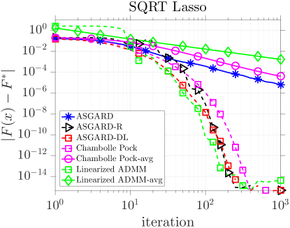
ALM, ADMM and Chambolle-Pock methods have the convergence rate guarantees in an ergodic sense. That is, they have the rate guarantees only on the averaged iterate sequence. In contrast, our guarantees are for the last iterate of the algorithm. To illustrate the importance between these two, we consider two synthetic problems in this section. The first one is a square root LASSO problem widely studied in the literature, which is given by:

F:=minxp{F(x):=Axb2+λx1},assignsuperscript𝐹subscript𝑥superscript𝑝assign𝐹𝑥subscriptnorm𝐴𝑥𝑏2𝜆subscriptnorm𝑥1F^{\star}:=\min_{x\in\mathbb{R}^{p}}\Big{\{}F(x):=\|Ax-b\|_{2}+\lambda\|x\|_{1}\Big{\}},

where An×p𝐴superscript𝑛𝑝A\in\mathbb{R}^{n\times p} is generated using a Gaussian distribution and is normalized such that column norms are equal to 1. Given a groundtruth vector xsuperscript𝑥x^{\natural}, we generate the observations as b=Ax+σ𝐧𝑏𝐴superscript𝑥𝜎𝐧b=Ax^{\natural}+\sigma\mathbf{n}, where 𝐧𝐧\mathbf{n} is a noise vector generated by a standard Gaussian distribution and σ=0.01𝜎0.01\sigma=0.01. We set λ=0.03𝜆0.03\lambda=0.03 which is tuned to get a good recovery of xsuperscript𝑥x^{\natural}.

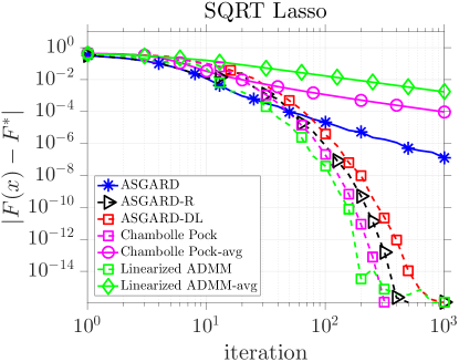
In this experiment, we test the ergodic and non-ergodic variants of Linearized ADMM (in the sense that the augmented term in the Lagrangian is linearized) gao2017first , and Chambolle-Pock’s algorithm Chambolle2011 . These methods have convergence guarantees for their last iterates, however, their rate guarantees only apply to the averaged sequence. Moreover, they are very successful to solve this type of problems as can be seen from the litterature. The behavior of the algorithms is given in Figure 1.
Refer to caption
Refer to caption
Figure 1: Performance of 5 algorithms for solving square root LASSO problem. Left: σ=0.1,λ=0.04formulae-sequence𝜎0.1𝜆0.04\sigma=0.1,\lambda=0.04, Right: σ=0.01,λ=0.03formulae-sequence𝜎0.01𝜆0.03\sigma=0.01,\lambda=0.03

As can be seen in Figure 1, last iterates of Linearized ADMM and Chambolle Pock’s algorithms seem to have the best performance. However, the averaged iterates for which the methods have the rate guarantees shows the slowest convergence behavior. Our method has the same rate as restarted ASGARD which does not have any convergence guarantees.

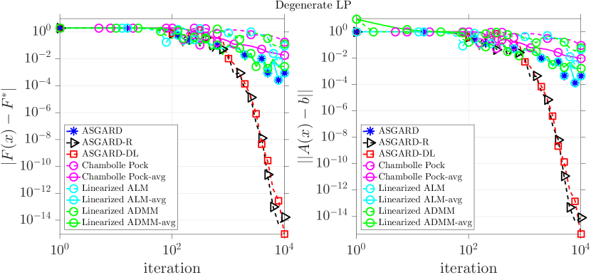
To illustrate the behavior of the last iterates of Linearized ADMM and Chambolle Pock’s algorithm, we consider a degenerate linear program which is also studied in TranDinh2015b :

minxp{h(x):=2xpk=1p1xk=1,xpk=1p1xk=0(2jn),xp0}.subscript𝑥superscript𝑝assign𝑥conditional2subscript𝑥𝑝superscriptsubscript𝑘1𝑝1subscript𝑥𝑘1subscript𝑥𝑝superscriptsubscript𝑘1𝑝1subscript𝑥𝑘02𝑗𝑛subscript𝑥𝑝0\min_{x\in\mathbb{R}^{p}}\Big{\{}h(x):=2x_{p}~{}\mid~{}~{}\sum_{k=1}^{p-1}x_{k}=1,~{}~{}x_{p}-\sum_{k=1}^{p-1}x_{k}=0~{}~{}(2\leq j\leq n),~{}~{}x_{p}\geq 0\Big{\}}.

The second inequality is repeated n1𝑛1n-1 times which causes the problem to be degenerate. We define the linear constraint as

Ax:=[k=1p1xk,xpk=1p1xk,,xpk=1p1xk].assign𝐴𝑥superscriptsuperscriptsubscript𝑘1𝑝1subscript𝑥𝑘subscript𝑥𝑝superscriptsubscript𝑘1𝑝1subscript𝑥𝑘subscript𝑥𝑝superscriptsubscript𝑘1𝑝1subscript𝑥𝑘topAx:=\Big{[}\sum_{k=1}^{p-1}x_{k},~{}~{}x_{p}-\sum_{k=1}^{p-1}x_{k},\cdots,~{}~{}x_{p}-\sum_{k=1}^{p-1}x_{k}\Big{]}^{\top}.

We have b:=(1,0,,0)nassign𝑏superscript100topsuperscript𝑛b:=\left(1,0,\cdots,0\right)^{\top}\in\mathbb{R}^{n}. We map the problem to our template in (31) as f(x):=δ{xp0}(xp)assign𝑓𝑥subscript𝛿subscript𝑥𝑝0subscript𝑥𝑝f(x):=\delta_{\left\{x_{p}\geq 0\right\}}(x_{p}), g(x):=δ{b}(Ax)assign𝑔𝑥subscript𝛿𝑏𝐴𝑥g(x):=\delta_{\left\{b\right\}}(Ax), and h(x):=2xpassign𝑥2subscript𝑥𝑝h(x):=2x_{p}. For this problem, we pick p=10𝑝10p=10 and n=200𝑛200n=200.

In addition to Linearized ADMM and Chambolle-Pock’s algorithm, we also include linearized ALM gao2017first to solve this example. The result of this test is given in Figure 2, where F(x)=h(x)𝐹𝑥𝑥F(x)=h(x).

Refer to caption
Figure 2: Performance of 6 algorithms for solving the degenerate linear program.

As can be seen from Figure 2, Linearized ADMM, Linearized ALM and Chambolle-Pock’s algorithm can get extremely slow where our algorithm and ASGARD with restart makes progress and converges to optimal value with a very high accuracy, and beyond the theoretical rate guarantee.

4.2 Basis Pursuit for recovering Bag-of-Words of text documents

We first consider a basis pursuit problem which is used in signal/image processing, statistics, and machine learning chen2001atomic ; donoho2006compressed ; candes2006robust :

minxp{F(x):=x1Ax=b},subscript𝑥superscript𝑝assign𝐹𝑥conditionalsubscriptnorm𝑥1𝐴𝑥𝑏\min_{x\in\mathbb{R}^{p}}\big{\{}F(x):=\|x\|_{1}~{}\mid~{}Ax=b\big{\}}, (35)

where An×p𝐴superscript𝑛𝑝A\in\mathbb{R}^{n\times p} and bn𝑏superscript𝑛b\in\mathbb{R}^{n}. This problem clearly fits into our template (1) by mapping f()=1f(\cdot)=\|\cdot\|_{1} and g()=δ{b}()𝑔subscript𝛿𝑏g(\cdot)=\delta_{\left\{b\right\}}(\cdot). It is also a special case of (3) with 𝒦={𝟎}𝒦0\mathcal{K}=\left\{\boldsymbol{0}\right\}. Proximal operators of both terms are given in a closed form.

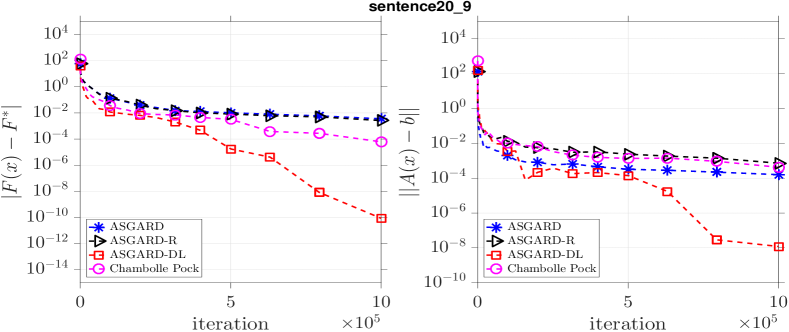
We apply this model to text processing. In arora2018a , the authors proposed using basis pursuit formulation to obtain bag-of-words representation from the unigram embedding representation of a text. The setting can be briefly described as the following: For any word w𝑤w, there exists a word vector vwnsubscript𝑣𝑤superscript𝑛v_{w}\in\mathbb{R}^{n}. For a given text document {w1,,wT}subscript𝑤1subscript𝑤𝑇\left\{w_{1},\cdots,w_{T}\right\}, one defines the unigram embedding as i=1Tvwisuperscriptsubscript𝑖1𝑇subscript𝑣subscript𝑤𝑖\sum_{i=1}^{T}v_{w_{i}}. It is easy to see that unigram embeddings can be written as a linear system Ax𝐴𝑥Ax where An×p𝐴superscript𝑛𝑝A\in\mathbb{R}^{n\times p} contains vwisubscript𝑣subscript𝑤𝑖v_{w_{i}} in the ithsuperscript𝑖𝑡i^{th} column and xp𝑥superscript𝑝x\in\mathbb{R}^{p} is the bag-of-words vector which counts the number of occurances of words in a text. This application is considered in text processing applications to obtain the original text document given the unigram embeddings white2016generating .

For this experiment, we have used the movie review dataset of maas-EtAl:2011:ACL-HLT2011 . We have selected 444 different documents and computed the unigram embeddings using pre-trained word embeddings from GloVe pennington2014glove with n=50𝑛50n=50 as the dimension of the word vectors and restricted the vocabulary size to p=10,000𝑝10000p=10,000 for getting faster results with all algorithms.

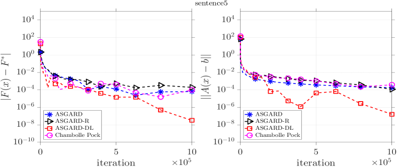
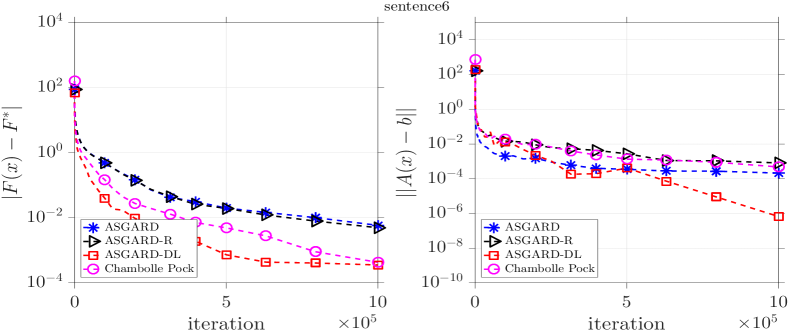
We have applied 444 methods to solve (35) for 444 different documents. Here, the parameter β0subscript𝛽0\beta_{0} in ASGARD, ASGARD-restart, and ASGARD-DL is set to β0:=10Aassignsubscript𝛽010norm𝐴\beta_{0}:=10\|A\|. Note that this choice is not optimal, but give us reasonable results in all test. The results are compiled in Figure 3.

Refer to caption
Refer to caption
Refer to caption
Refer to caption
Figure 3: Performance of 4 algorithms for solving basis pursuit for 4 text documents.

As we can observe from Figure 3, our new algorithm works quite well and is comparable with state-of-the-art methods for low accuracy. It outperforms them if we run the algorithms long enough to get more accurate solutions than ε=105𝜀superscript105\varepsilon=10^{-5} both in objective residual and feasibility. Note that (35) is fully nonsmooth, and A𝐴A is non-orthogonal. If we apply ADMM to solve (35), then it requires to solve a general convex subproblem, or a linear system, which has higher per-iteration complexity than four methods we used in this example.

4.3 The 1subscript1\ell_{1}-Regularized Least Absolute Deviation Problem (LAD)

Our second example is the 1subscript1\ell_{1}-regularized least absolute deviation regression problem, also known as LAD-Lasso in the literature. It is known that when the noise has a heavy tailed distribution such as Laplace distribution, LAD-Lasso is more robust to the outliers wang2007robust . The optimization model of this problem is

minxp{F(x):=Axb1+λx1},subscript𝑥superscript𝑝assign𝐹𝑥subscriptnorm𝐴𝑥𝑏1𝜆subscriptnorm𝑥1\min_{x\in\mathbb{R}^{p}}\Big{\{}F(x):=\left\|Ax-b\right\|_{1}+\lambda\left\|x\right\|_{1}\Big{\}}, (36)

where An×p𝐴superscript𝑛𝑝A\in\mathbb{R}^{n\times p} is generated according to a normal distribution and the noise 𝐧n𝐧superscript𝑛\mathbf{n}\in\mathbb{R}^{n} is generated by Laplace(0,1)01(0,1) distribution. We generate an observed vector b:=Ax+σ𝐧assign𝑏𝐴superscript𝑥𝜎𝐧b:=Ax^{\natural}+\sigma\mathbf{n}, where σ:=0.1assign𝜎0.1\sigma:=0.1 and xsuperscript𝑥x^{\natural} is a s𝑠s-sparse vector of ground-truth. We choose λ:=1/nassign𝜆1𝑛\lambda:=1/n for the regularization parameter, which gives us a good recovery of xsuperscript𝑥x^{\natural}.

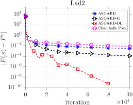
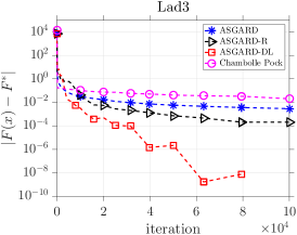
This problem fits to our template by setting f():=λ1f(\cdot):=\lambda\|\cdot\|_{1} and g()=b1g(\cdot)=\|\cdot-b\|_{1}. We set β0subscript𝛽0\beta_{0} in ASGARD, ASGARD-restart, and ASGARD-DL as β0:=100Aassignsubscript𝛽0100norm𝐴\beta_{0}:=100\|A\|. We generated three problem instances of the size n:=340rassign𝑛340𝑟n:=340r, p:=1000rassign𝑝1000𝑟p:=1000r, s:=100rassign𝑠100𝑟s:=100r, where s𝑠s is the sparsity level, and r=1,2,3𝑟123r=1,2,3 for the first, second and third instances, respectively. We present the results of this example in Figure 4.
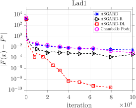
Refer to caption Refer to caption Refer to caption
Figure 4: Performance of 4 algorithms for LAD-Lasso problem in 3 different realization of varying problem size.

As we can see from Figure 4 that, with the same per-iteration complexity, our method significantly outperforms the other algorithms after accuracy 104superscript10410^{-4}. It beats other algorithms after a couple of hundred iterations and continues to decrease the objective values. Although this problem is fully nonsmooth, heuristic restart such as in ASGARD still improves the performance of the non-restart one, but does not significant outperform.

4.4 Support Vector Machines

Our next example is the following primal support vector machines (SVM) problem in binary classification. Instead of classical models, we consider the following 1subscript1\ell_{1}-regularized nonsmooth hinge loss as proposed in zhu20041 :

minxp{F(x):=1ni=1nmax{0,1biai,x}+λx1},subscript𝑥superscript𝑝assign𝐹𝑥1𝑛superscriptsubscript𝑖1𝑛01subscript𝑏𝑖subscript𝑎𝑖𝑥𝜆subscriptnorm𝑥1\min_{x\in\mathbb{R}^{p}}\Big{\{}F(x):=\frac{1}{n}\sum_{i=1}^{n}\max\left\{0,1-b_{i}\langle a_{i},x\rangle\right\}+\lambda\|x\|_{1}\Big{\}}, (37)

where aipsubscript𝑎𝑖superscript𝑝a_{i}\in\mathbb{R}^{p} are the feature vectors and bi{1,+1}subscript𝑏𝑖11b_{i}\in\{-1,+1\} are the labels for i=1,,n𝑖1𝑛i=1,\cdots,n. We can cast (37) into our template by setting f():=λ1f(\cdot):=\lambda\|\cdot\|_{1} and

g(Ax)=1ni=1nmax{0,1biai,x}=maxy[0,1]ny,Ax+1n𝟙,𝑔𝐴𝑥1𝑛superscriptsubscript𝑖1𝑛01subscript𝑏𝑖subscript𝑎𝑖𝑥subscript𝑦superscript01𝑛𝑦𝐴𝑥1𝑛1g(Ax)=\frac{1}{n}\sum_{i=1}^{n}\max\{0,1-b_{i}\langle a_{i},x\rangle\}=\max_{y\in[0,1]^{n}}\langle y,Ax+\frac{1}{n}\mathbbm{1}\rangle,

where A:=1n[b1a1,b2a2,,bnan]assign𝐴1𝑛superscriptmatrixsubscript𝑏1subscript𝑎1subscript𝑏2subscript𝑎2subscript𝑏𝑛subscript𝑎𝑛topA:=-\frac{1}{n}\begin{bmatrix}b_{1}a_{1},b_{2}a_{2},\cdots,b_{n}a_{n}\end{bmatrix}^{\top} and 𝟙1\mathbbm{1} is a vector of all ones. Clearly, the proximal operator of g𝑔g is simply a projection onto [0,1]nsuperscript01𝑛[0,1]^{n}.

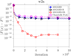
We use 10 different datasets from libsvm CC01a to test four different algorithms. The initial value β0subscript𝛽0\beta_{0} in ASGARD, ASGARD-restart, and ASGARD-DL is set to β0:=0.1Aassignsubscript𝛽00.1norm𝐴\beta_{0}:=0.1\|A\|. But for covtype dataset, we used β0:=0.01Aassignsubscript𝛽00.01norm𝐴\beta_{0}:=0.01\|A\|. The details about the datasets are given in Table 1.

Table 1: Datasets used for classification.
Data set Training size Number of features
w1a 2,477 300
w2a 3,470 300
w3a 4,912 300
w4a 7,366 300
w5a 9,888 300
w6a 17,188 300
w7a 24,692 300
w8a 49,749 300
rcv1 20,242 47,236
covtype 581,012 54

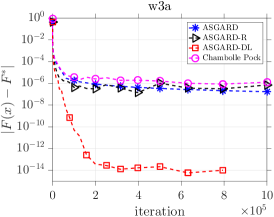
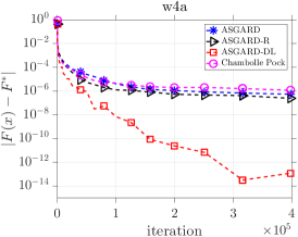
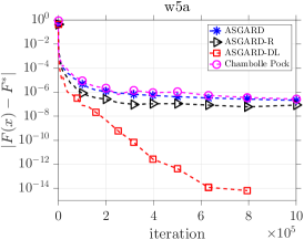
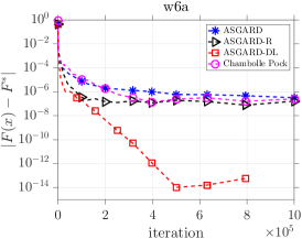
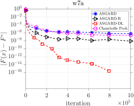
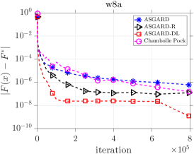
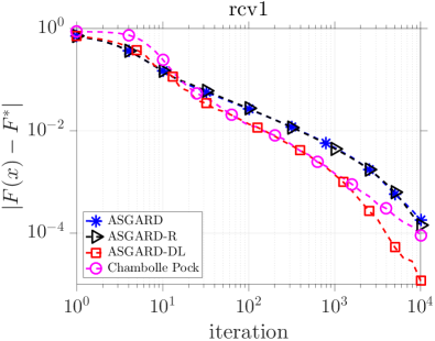
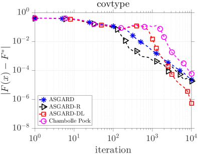
We test 444 algorithms on these ten datasets. The results of the first 888 problems are given in Figure 5, and the results of the two last problems are in Figure 6.

Refer to caption Refer to caption Refer to caption
Refer to caption Refer to caption
Figure 5: Performance of 444 algorithms for the 1subscript1\ell_{1}-regularized SVM problem on {w1a,,w8a}w1aw8a\left\{\texttt{w1a},\cdots,\texttt{w8a}\right\}.
Refer to caption Refer to caption
Figure 6: Performance of 444 algorithms for the 1subscript1\ell_{1}-regularized SVM problem on {rcv1,covtype}rcv1covtype\left\{\texttt{rcv1},\texttt{covtype}\right\}.

We again observe that Algorithm 2 significantly outperform the other methods. Since these algorithms have the same per-iteration complexity, it is sufficient to compare them in terms of iteration numbers. Although all the algorithms have 𝒪(1k)𝒪1𝑘\mathcal{O}\left(\frac{1}{k}\right)-worst-case convergence rate, due to its double-loop, Algorithm 2 performs much better than the others, especially for high accurate solutions. This is not surprise. The double-loop allows Algorithm 1 to use large stepsize by frequently restarting τksubscript𝜏𝑘\tau_{k} and βksubscript𝛽𝑘\beta_{k}, while ASGARD gradually decreases these parameters to zero, and Chambolle-Pock’s method fixes the step-size. Note that the 𝒪(1k)𝒪1𝑘\mathcal{O}\left(\frac{1}{k}\right) rate of Chambolle-Pock’s method is achieved via the averaging sequence, which is often much slower than the last iteration as we showed in Figures 5 and 6.

4.5 Markowitz Portfolio Optimization

We consider a classical example from Markowitz portfolio optimization brodie2009sparse . The setting we consider here aims at maximizing the expected return for a given risk level. Assume that we are given a vector ρn𝜌superscript𝑛\rho\in\mathbb{R}^{n}, where ρ𝜌\rho is composed of expected returns from n𝑛n assets. This problem can be formulated as

maxxp{ρxx,𝔼[|(aiρ)x|2]ϵ},subscript𝑥superscript𝑝conditionalsuperscript𝜌top𝑥𝑥𝔼delimited-[]superscriptsuperscriptsubscript𝑎𝑖𝜌top𝑥2italic-ϵ\max_{x\in\mathbb{R}^{p}}\Big{\{}\rho^{\top}x~{}\mid~{}x\in\triangle,~{}\mathbb{E}\left[|(a_{i}-\rho)^{\top}x|^{2}\right]\leq\epsilon\Big{\}}, (38)

For our setting, we use empirical sample average instead of the expectation and convert the problem to a minimization problem by negating the objective:

minxp{ρ,xx,1pAx22ϵ},subscript𝑥superscript𝑝conditional𝜌𝑥𝑥1𝑝superscriptsubscriptnorm𝐴𝑥22italic-ϵ\min_{x\in\mathbb{R}^{p}}\left\{-\langle\rho,x\rangle~{}\mid~{}x\in\triangle,~{}\tfrac{1}{p}\|Ax\|_{2}^{2}\leq\epsilon\right\}, (39)

where A=[(a1ρ),(a2ρ),,(anρ)]𝐴superscriptsubscript𝑎1𝜌subscript𝑎2𝜌subscript𝑎𝑛𝜌topA=[(a_{1}-\rho),(a_{2}-\rho),\dots,(a_{n}-\rho)]^{\top}. We map this problem to our template (31) by mapping f():=δ()assign𝑓subscript𝛿f(\cdot):=\delta_{\triangle}(\cdot), g():=δ{2pϵ}()g(\cdot):=\delta_{\left\{\left\|\cdot\right\|_{2}\leq\sqrt{p\epsilon}\right\}}(\cdot), and h(x):=ρ,xassign𝑥𝜌𝑥h(x):=-\langle\rho,x\rangle. One key step of primal-dual algorithms is computing the projection onto an 2subscript2\ell_{2}-norm ball and on a simplex. Here, the complexity of simplex projection is 𝒪(plogp)𝒪𝑝𝑝\mathcal{O}(p\log p).

As before, we apply 444 algorithms to solve (38). We use 444 datasets that are also considered in borodin2004can . The details about the datasets are given in Table 2.

Table 2: Portfolio optimization datasets and parameters of algorithms.
The size of datasets Parameters used in 444 algorithms.
Datasets n𝑛n p𝑝p ϵitalic-ϵ\epsilon in (39) β0subscript𝛽0\beta_{0} RF ω𝜔\omega mssubscript𝑚𝑠m_{s} τ𝜏\tau σ𝜎\sigma
DJIA 507 30 0.002 Anorm𝐴\|A\| 10 1.1 11 1A1norm𝐴\frac{1}{\|A\|} 1A1norm𝐴\frac{1}{\|A\|}
NYSE 5651 36 0.02 100A100norm𝐴100\|A\| 10 1.1 11 1A1norm𝐴\frac{1}{\|A\|} 1A1norm𝐴\frac{1}{\|A\|}
SP500 1276 25 0.02 100A100norm𝐴100\|A\| 10 1.2 6 1A1norm𝐴\frac{1}{\|A\|} 1A1norm𝐴\frac{1}{\|A\|}
TSE 1258 88 0.002 100A100norm𝐴100\|A\| 10 1.1 11 1A1norm𝐴\frac{1}{\|A\|} 1A1norm𝐴\frac{1}{\|A\|}

We summarized the parameters that we used for these algorithms in Table 2, where β0subscript𝛽0\beta_{0} is common to ASGARD, ASGARD-restart, our algorithm, restart frequency (RF) is specific to ASGARD-restart, ω𝜔\omega and mssubscript𝑚𝑠m_{s} are specific to our algorithm and τ𝜏\tau and σ𝜎\sigma are specific to Chambolle-Pock’s algorithm.
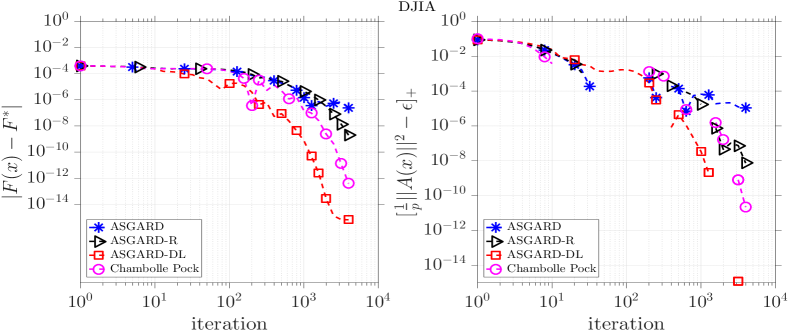
Refer to caption
Refer to caption
Refer to caption
Refer to caption
Figure 7: Performance of 4 algorithms for Markowitz portfolio optimization problem on 4 real datasets.

We have tested 4 algorithms on 4 real datasets and the results are compiled in Figure 7. As can be seen, except for SP500 dataset, Algorithm 2 significantly outperforms the other methods and shows a much faster practical performance than 𝒪(1k)𝒪1𝑘\mathcal{O}\left(\frac{1}{k}\right) guarantee. For SP500 dataset, ASGARD-restart algorithm shows a comparable performance to our method. However, as discussed in TranDinh2015b , the effect of restarting to ASGARD method is not understood theoretically. Our algorithm theoretically preserves the best-known 𝒪(1k)𝒪1𝑘\mathcal{O}\left(\frac{1}{k}\right) guarantee while performing as fast as, and most of the times faster than the heuristic restarting ASGARD method.

4.6 Sparse Subspace Clustering

In the last example, we consider the following sparse subspace clustering problem which has broad applications in machine learning, computer vision and image processing. This problem is studied extensively in the literature elhamifar2013sparse ; elhamifar2009sparse ; pourkamali2018efficient . In this problem setting, we assume that there exist n𝑛n points {x1,x2,,xn}psubscript𝑥1subscript𝑥2subscript𝑥𝑛superscript𝑝\left\{x_{1},x_{2},\cdots,x_{n}\right\}\in\mathbb{R}^{p} lying in the union of subspaces in psuperscript𝑝\mathbb{R}^{p}. We form a matrix Xp×n𝑋superscript𝑝𝑛X\in\mathbb{R}^{p\times n} by stacking {x1,x2,,xn}subscript𝑥1subscript𝑥2subscript𝑥𝑛\left\{x_{1},x_{2},\cdots,x_{n}\right\} as the columns. With this notation, each point can be represented as

xj=Xcj+ej,s.t.[cj]j=0and𝟙cj=1.formulae-sequencesubscript𝑥𝑗𝑋subscript𝑐𝑗subscript𝑒𝑗s.t.subscriptdelimited-[]subscript𝑐𝑗𝑗0andsuperscript1topsubscript𝑐𝑗1x_{j}=Xc_{j}+e_{j},~{}~{}\text{s.t.}~{}~{}[c_{j}]_{j}=0~{}~{}\text{and}~{}~{}\mathbbm{1}^{\top}c_{j}=1.

where cjnsubscript𝑐𝑗superscript𝑛c_{j}\in\mathbb{R}^{n} represents the coefficients to represent point xjpsubscript𝑥𝑗superscript𝑝x_{j}\in\mathbb{R}^{p} as an affine combination of other points, ejpsubscript𝑒𝑗superscript𝑝e_{j}\in\mathbb{R}^{p} is the representation error and 𝟙n1superscript𝑛\mathbbm{1}\in\mathbb{R}^{n} is a vector of 111’s.

This formulation can be represented compactly by stacking cjsubscript𝑐𝑗c_{j} to the jthsuperscript𝑗thj^{\text{th}} column of matrix C𝐶C as follows:

X=CXs.t.diag(C)=0,C𝟙=𝟙.formulae-sequence𝑋𝐶𝑋s.t.diag𝐶0superscript𝐶top11X=CX~{}~{}\text{s.t.}~{}~{}\mathrm{diag}(C)=0,~{}C^{\top}\mathbbm{1}=\mathbbm{1}. (40)

The optimization problem that we will tackle in this subsection is referred to as an SSC-Lasso problem in the literature, and is written as

minCn×n{C1+λ2XCX2diag(C)=0,C𝟙=𝟙}.subscript𝐶superscript𝑛𝑛subscriptnorm𝐶1conditional𝜆2superscriptnorm𝑋𝐶𝑋2diag𝐶0superscript𝐶top11\min_{C\in\mathbb{R}^{n\times n}}\Big{\{}\left\|C\right\|_{1}+\tfrac{\lambda}{2}\left\|X-CX\right\|^{2}~{}\mid~{}\mathrm{diag}(C)=0,~{}C^{\top}\mathbbm{1}=\mathbbm{1}\Big{\}}. (41)

In elhamifar2009sparse and elhamifar2013sparse , ADMM is used to solve (41) and recently, pourkamali2018efficient proposed an efficient implementation of ADMM and an application of standard accelerated proximal scheme to this setting. One drawback of applying accelerated proximal schemes to (41) is the evaluation of the proximal operator of an 1subscript1\ell_{1}-norm over the linear constraint C𝟙=𝟙superscript𝐶top11C^{\top}\mathbbm{1}=\mathbbm{1}. This requires additional computation cost of log(n)pn2𝑛𝑝superscript𝑛2\log(n)pn^{2}. We fit (41) into our template (31) by defining f():=1+δ{diag()=0}()f(\cdot):=\|\cdot\|_{1}+\delta_{\left\{\mathrm{diag}(\cdot)=0\right\}}(\cdot), g():=δ{,𝟙=𝟙}()assign𝑔subscript𝛿11g(\cdot):=\delta_{\left\{\langle\cdot,\mathbbm{1}\rangle=\mathbbm{1}\right\}}(\cdot), and h()=λ2XX()2𝜆2superscriptnorm𝑋𝑋2h(\cdot)=\frac{\lambda}{2}\|X-X(\cdot)\|^{2}. If we apply Algorithm 2 to solve this reformulation, then no extra computation cost is incurred as in accelerated proximal gradient methods.

We use a classic benchmark Extended Yale B dataset georghiades2001few to test the sparse subspace clustering problem (41). This dataset contains face pictures of 383838 individuals taken under 646464 different environmental conditions. As previous works, we use downsampled images of size 48×42484248\times 42 pixels which correspond to p=2016𝑝2016p=2016. We ran experiments with ADMM, TFOCS, and our method ASGARD-DL. We note that our method includes tuning parameters similar to ADMM. We use β0:=Massignsubscript𝛽0norm𝑀\beta_{0}:=\sqrt{\|M\|}, where M(C)=C𝟙𝑀𝐶superscript𝐶top1M(C)=C^{\top}\mathbbm{1}. We randomly selected m=2,3,5𝑚235m=2,3,5 clusters and ran 333 trials for each case. We have used the implementation of ADMM elhamifar2013sparse ; elhamifar2009sparse and TFOCS pourkamali2018efficient provided by the authors of pourkamali2018efficient ; elhamifar2013sparse ; elhamifar2009sparse . For fair comparison, we ran the algorithms for the same duration of time and reported the results accordingly. We used objective value and clustering error as comparison measures as pourkamali2018efficient .

Table 3: Comparison of 3 methods on the SSC-Lasso problem with m=2,3,5𝑚235m=2,3,5 clusters and 333 independent trials of each.
Problem ADMM TFOCS ASGARD-DL
(n=2𝑛2n=2)-objective-trial 1 236.5653 226.4371 225.7578
(n=2𝑛2n=2)-Clustering error-trial 1 0.0312 0.0391 0.0391
(n=2𝑛2n=2)-objective-trial 2 200.3710 192.2985 191.5177
(n=2𝑛2n=2)-Clustering error-trial 2 0.0234 0.0469 0.0469
(n=2𝑛2n=2)-objective-trial 3 197.2510 188.7655 188.1555
(n=2𝑛2n=2)-Clustering error-trial 3 0.0703 0.0938 0.0938
(n=3𝑛3n=3)-objective-trial 1 329.9188 320.9690 319.5887
(n=3𝑛3n=3)-Clustering error-trial 1 0.0156 0.0156 0.0312
(n=3𝑛3n=3)-objective-trial 2 341.1980 330.6395 329.5704
(n=3𝑛3n=3)-Clustering error-trial 2 0.0729 0.0677 0.0677
(n=3𝑛3n=3)-objective-trial 3 398.8778 389.3963 388.0739
(n=3𝑛3n=3)-Clustering error-trial 3 0.4375 0.3594 0.3646
(n=5𝑛5n=5)-objective-trial 1 549.8250 530.0340 526.1905
(n=5𝑛5n=5)-Clustering error-trial 1 0.1625 0.1156 0.0906
(n=5𝑛5n=5)-objective-trial 2 482.8483 467.0535 461.6563
(n=5𝑛5n=5)-Clustering error-trial 2 0.2188 0.1125 0.1562
(n=5𝑛5n=5)-objective-trial 3 1029.5459 1017.7089 1025.6752
(n=5𝑛5n=5)-Clustering error-trial 3 0.3156 0.3469 0.3156

We can see from Table 3 that our method consistently outperforms other methods in terms of objective values, and has similar performance in terms of the clustering error. We present our algorithm as another candidate for solving the classical sparse subspace clustering problem with a lower per iteration cost than previous approaches ADMM and TFOCS and similar performance.

5 Further discussion and comparison with previous work

Theory and numerical methods for solving (1) and (3) are well-studied in the literature. Due to such a large proportion of solution methods, we only focus on some recent works that are the most related to our method developed in this paper. We briefly survey these results to highlight the similarities and differences with our work.

In Nesterov2005c , Nesterov proposed combining smoothing technique and accelerated gradient methods to obtain 𝒪(1ε)𝒪1𝜀\mathcal{O}\left(\frac{1}{\varepsilon}\right)-iteration complexity to obtain an ε𝜀\varepsilon-approximate solution to (1). However, this method requires ε𝜀\varepsilon to be predefined, and both primal and dual domains are bounded. In addition, the step-size of the underlying gradient-type scheme is proportional to ε𝜀\varepsilon, which is often small. This leads to a poor performance in early iterations. In Nesterov2005d , Nesterov introduced an excessive gap technique to develop new algorithms that allow the smoothness parameter to be adaptively updated. Nevertheless, these methods still require both primal and dual domains to be bounded, and one additional proximal operator for every two iterations.

In  Chambolle2011 ; chambolle2016ergodic , A. Chambolle and T. Pock proposed a primal-dual algorithm to solve (1) that achieves 𝒪(1k)𝒪1𝑘\mathcal{O}\left(\frac{1}{k}\right)-convergence rate. This rate is guaranteed on a gap function and also requires both primal and dual domains to be bounded, which is unfortunately not applicable to (3). In addition, the guarantee of their methods relies on ergodic or weighted averaging sequences. Note that, in sparse and low-rank optimization and image processing, taking averaging sequence unfortunately destroys desired structures of approximate solutions. In addition, as also presented with numerical evidence, averaging sequences perform poorly in practice.

In xu2016homotopy , the authors proposed a homotopy algorithm called Homotopy Smoothing algorithm (HOPS) which also essentially relies on Nesterov’s smoothing technique Nesterov2005c . HOPS employs a similar strategy to ours in the sense of having a double loop structure. However, this method suffers from several drawbacks. First, it only applies to unconstrained problems as in (1), but not to (3) due to the unboundedness of the dual domain. Second, it requires knowing ε0=P(x0)P(x)subscript𝜀0𝑃superscript𝑥0𝑃superscript𝑥\varepsilon_{0}=P(x^{0})-P(x^{\star}) to be able to set the initial smoothness parameter. Third, HOPS requires tuning the number of inner iterations and the rate at which the smoothness parameter is going to be reduced. The alternative of HOPS to alleviate this issue requires a bounded primal domain which further restricts the usage of their method.

Table 4: Summary of algorithms that require two proximal operators each iteration. Note that zk:=k=1Kwkxkassignsuperscript𝑧𝑘superscriptsubscript𝑘1𝐾superscript𝑤𝑘superscript𝑥𝑘z^{k}:=\sum_{k=1}^{K}w^{k}x^{k} where K is the maximum number of iterations and wksuperscript𝑤𝑘w^{k} are the weights. For solving the unconstrained problem with ALM/ADMM methods, we split the problem. Practicality column refers to whether using the iterate in the convergence rate gives a fast practical performance or not.
Algorithm g𝑔g is Lipschitz g=δ{b}𝑔subscript𝛿𝑏g=\delta_{\{b\}} Type of rate Set ϵitalic-ϵ\epsilon Practicality
Nesterov Nesterov2005c P(xk)P𝒪(max(ϵ,1ϵk2))𝑃superscript𝑥𝑘superscript𝑃𝒪italic-ϵ1italic-ϵsuperscript𝑘2P(x^{k})-P^{\star}\leq\mathcal{O}\left(\max\left(\epsilon,\frac{1}{\epsilon k^{2}}\right)\right) Not applicable Non-ergodic Yes No
Chambolle-Pock Chambolle2011 G(zk)𝒪(1k)𝐺superscript𝑧𝑘𝒪1𝑘G(z^{k})\leq\mathcal{O}\left(\frac{1}{k}\right) Convergence Ergodic No No
Linearized ALM xu2017accelerated P(zk)P𝒪(1k)𝑃superscript𝑧𝑘superscript𝑃𝒪1𝑘P(z^{k})-P^{\star}\leq\mathcal{O}\left(\frac{1}{k}\right) |f(zk)f|𝒪(1k)𝑓superscript𝑧𝑘superscript𝑓𝒪1𝑘\displaystyle|f(z^{k})-f^{\star}|\leq\mathcal{O}\left(\frac{1}{k}\right) Axb𝒪(1k)norm𝐴𝑥𝑏𝒪1𝑘\displaystyle\|Ax-b\|\leq\mathcal{O}\left(\frac{1}{k}\right) Ergodic No No
Inexact ALM xu2017iteration P(zk)P𝒪(max(ϵk,βk))𝑃superscript𝑧𝑘superscript𝑃𝒪subscriptitalic-ϵ𝑘subscript𝛽𝑘P(z^{k})-P^{\star}\leq\mathcal{O}\left(\max\left(\epsilon_{k},\beta_{k}\right)\right) |f(zk)f|𝒪(max(ϵk+βk))𝑓superscript𝑧𝑘superscript𝑓𝒪subscriptitalic-ϵ𝑘subscript𝛽𝑘\displaystyle|f(z^{k})-f^{\star}|\leq\mathcal{O}\left(\max\left(\epsilon_{k}+\beta_{k}\right)\right) Axb𝒪(βk)norm𝐴𝑥𝑏𝒪subscript𝛽𝑘\displaystyle\|Ax-b\|\leq\mathcal{O}\left(\beta_{k}\right)~{}~{}~{}~{}~{}~{}~{}~{}~{}~{} Non-ergodic Yes No
Linearized ADMM xu2017accelerated P(z1k,z2k)P=𝒪(1k)𝑃superscriptsubscript𝑧1𝑘superscriptsubscript𝑧2𝑘superscript𝑃𝒪1𝑘P(z_{1}^{k},z_{2}^{k})-P^{\star}=\mathcal{O}\left(\frac{1}{k}\right) |f1(z1k)+f2(z2k)f1f2|𝒪(1k)subscript𝑓1superscriptsubscript𝑧1𝑘subscript𝑓2superscriptsubscript𝑧2𝑘superscriptsubscript𝑓1superscriptsubscript𝑓2𝒪1𝑘\displaystyle|f_{1}(z_{1}^{k})+f_{2}(z_{2}^{k})-f_{1}^{\star}-f_{2}^{\star}|\leq\mathcal{O}\left(\frac{1}{k}\right) A1z1k+A2z2kb𝒪(1k)normsubscript𝐴1superscriptsubscript𝑧1𝑘subscript𝐴2superscriptsubscript𝑧2𝑘𝑏𝒪1𝑘\displaystyle\|A_{1}z_{1}^{k}+A_{2}z_{2}^{k}-b\|\leq\mathcal{O}\left(\frac{1}{k}\right) Ergodic No No
ASGARD TranDinh2015b P(xk)P𝒪(1k)𝑃superscript𝑥𝑘superscript𝑃𝒪1𝑘P(x^{k})-P^{\star}\leq\mathcal{O}\left(\frac{1}{k}\right) |f(xk)f|𝒪(1k)𝑓superscript𝑥𝑘superscript𝑓𝒪1𝑘\displaystyle|f(x^{k})-f^{\star}|\leq\mathcal{O}\left(\frac{1}{k}\right) Axkb𝒪(1k)norm𝐴superscript𝑥𝑘𝑏𝒪1𝑘\displaystyle\|Ax^{k}-b\|\leq\mathcal{O}\left(\frac{1}{k}\right) Non-ergodic No No
This paper (Algorithm 2) P(xk)P𝒪(1k)𝑃superscript𝑥𝑘superscript𝑃𝒪1𝑘P(x^{k})-P^{\star}\leq\mathcal{O}\left(\frac{1}{k}\right) |f(xk)f|𝒪(1k)𝑓superscript𝑥𝑘superscript𝑓𝒪1𝑘\displaystyle|f(x^{k})-f^{\star}|\leq\mathcal{O}\left(\frac{1}{k}\right) Axkb𝒪(1k)norm𝐴superscript𝑥𝑘𝑏𝒪1𝑘\displaystyle\|Ax^{k}-b\|\leq\mathcal{O}\left(\frac{1}{k}\right) Non-ergodic No Yes

For constrained problem (3), among different methods, augmented Lagrangian (ALM), alternating direction method of multipliers (ADMM), alternating minimization algorithms (AMA), and penalty methods are the most popular. Inexact augmented Lagrangian methods (iALM) lan2016iteration ; nedelcu2014computational ; xu2017iteration relies on a double loop structure similar to our method. However, termination rules for these methods require the desired accuracy ε𝜀\varepsilon to be set a priori. In addition, in practice, it is not easy to check when the inner problem is solved to an εksubscript𝜀𝑘\varepsilon_{k}-accuracy in the k𝑘k-th iteration. Such an estimate is often derived from the worst-case complexity bound of the underlying solution method, and therefore, the corresponding algorithm is not efficient in practice.

While ADMM works really well and is widely used in practice, AMA is rarely used and requires additional conditions to converge. The best-known convergence rate of ADMM and its variants such as linearized ADMM and preconditioned ADMM is 𝒪(1k)𝒪1𝑘\mathcal{O}\left(\frac{1}{k}\right) under standard assumptions He2012 ; Monteiro2012b ; Monteiro2010 ; ouyang2015accelerated ; xu2017accelerated . Moreover, this rate is given in an ergodic sense, and examples show that such a rate is optimal. See Boyd2011 for more information about the behavior of ADMM. In practice, however, the ergodic rate is rather pessimistic, which is much slower than the last iterate sequence (see Subsection 4.1 as an example). So far, we are not aware of any work showing an 𝒪(1k)𝒪1𝑘\mathcal{O}\left(\frac{1}{k}\right)-rate of the standard ADMM or its linearized and preconditioned ADMM in the last iterate. A recent work li2016accelerated combined preconditioned/linearized ADMM and Nesterov’s accelerated schemes to achieve an 𝒪(1k)𝒪1𝑘\mathcal{O}\left(\frac{1}{k}\right)-non-ergodic convergence rate.

Penalty methods use a quadratic penalty term to move the constraints to the objective and solve the subproblems by changing the penalty parameter lan2013iteration ; necoara2015complexity . Similar to iALM, these methods also do not have clear implementable termination rules for the inner loop. In addition, they do not involve dual variables. Therefore, they are often less competitive with primal-dual methods. A recent work tran2017proximal proposed a new alternating quadratic penalty algorithm to solve (3) that has the same 𝒪(1k)𝒪1𝑘\mathcal{O}\left(\frac{1}{k}\right)-non-ergodic convergence rate as in this paper. Nevertheless, this method is completely different from this paper and does not have an update on the dual center.

Compared to our previous work TranDinh2015b , ASGARD, our new algorithm shares some similarities but also has several differences. First, it has inner and outer loops but the guarantee is on the overall iterations. Second, it works with any Bregman divergence induced by a general prox-function when solving (1), while ASGARD only works with the Bregman distances induced by a strongly convex and Lipschitz gradient prox-function. This excludes some important Bregman divergences such as the Kullback-Leibler (KL) divergence. Third, our algorithm allows us to use different norms while computing proximal operators, compared to ASGARD which works with only Euclidean norms. Fourth, it automatically restarts both the primal and dual variables as well as the parameters. It also has a rigorous convergence guarantee, while the practical restarting variant of ASGARD does not have convergence guarantee.

We developed a novel analysis for our double loop structured smoothing algorithm which allowed us to derive flexible rules for parameters in both unconstrained and constrained problems, in contrast to xu2016homotopy . Our analysis gives insights on the heuristic restarting strategies in TranDinh2015b as well as on the number of inner iterations in the algorithm. It also gives explicit number of iterations for the inner subproblems and does not require to predefine the horizon as opposed to iALM. Table 5 summarizes the key differences between different methods we have discussed in this paper.

Table 5: A comparison with previous work (((β𝛽\beta is a smoothness parameter defined in (10)))).
ADMM/iALM Penalty / HOPS / ASGARD This work
Constant or adaptive β𝛽\beta. Analytically drive β𝛽\beta to 0. Analytically drive β𝛽\beta to 0.
Update the dual center. Do not move the dual center. Update the dual center.
Theory is driven by the convergence in the dual. Do not analyze the convergence of the dual. Only analyze the stability of the primal-dual sequence.
Inner problems are solved inexactly. Inner problems are solved inexactly. Only ensure stability for the number of inner iterations and smoothness parameter.

6 Convergence analysis: The proof of Theorems 3.1 and 3.2

We present the full proof of Theorems 3.1 and 3.2 in this section.

6.1 The proof of Theorem 3.1: Convergence of Algorithm 2 for (1)

With the same argument as in (TranDinh2015b, , Lemma 11), we can prove the following estimate at the k𝑘k-th iteration at the state s𝑠s of the outer loop, i.e., Ksk<Ks+1:=Ks+mssubscript𝐾𝑠𝑘subscript𝐾𝑠1assignsubscript𝐾𝑠subscript𝑚𝑠K_{s}\leq k<K_{s+1}:=K_{s}+m_{s}, of Algorithm 2:

Sβs(x¯k+1;y˙s)+τk2A2βsd𝒳(x,x^k+1)(1τk)Sβs(x¯k;y˙s)+τk2A2βsd𝒳(x,x^k)subscript𝑆subscript𝛽𝑠superscript¯𝑥𝑘1superscript˙𝑦𝑠superscriptsubscript𝜏𝑘2superscriptnorm𝐴2subscript𝛽𝑠subscript𝑑𝒳superscript𝑥superscript^𝑥𝑘11subscript𝜏𝑘subscript𝑆subscript𝛽𝑠superscript¯𝑥𝑘superscript˙𝑦𝑠superscriptsubscript𝜏𝑘2superscriptnorm𝐴2subscript𝛽𝑠subscript𝑑𝒳superscript𝑥superscript^𝑥𝑘\displaystyle S_{\beta_{s}}(\bar{x}^{k+1};\dot{y}^{s})+\tfrac{\tau_{k}^{2}\|A\|^{2}}{\beta_{s}}d_{\mathcal{X}}(x^{\star},\hat{x}^{k+1})\leq(1-\tau_{k})S_{\beta_{s}}(\bar{x}^{k};\dot{y}^{s})+\tfrac{\tau_{k}^{2}\|A\|^{2}}{\beta_{s}}d_{\mathcal{X}}(x^{\star},\hat{x}^{k})\vspace{1ex}
τkβsb𝒴(yβs(Ax~k;y˙s),y˙s)(1τk)βs2yβs(Ax~k;y˙s)yβs(Ax¯k;y˙s)𝒴2,subscript𝜏𝑘subscript𝛽𝑠subscript𝑏𝒴subscriptsuperscript𝑦subscript𝛽𝑠𝐴superscript~𝑥𝑘superscript˙𝑦𝑠superscript˙𝑦𝑠1subscript𝜏𝑘subscript𝛽𝑠2superscriptsubscriptnormsubscriptsuperscript𝑦subscript𝛽𝑠𝐴superscript~𝑥𝑘superscript˙𝑦𝑠subscriptsuperscript𝑦subscript𝛽𝑠𝐴superscript¯𝑥𝑘superscript˙𝑦𝑠𝒴2\displaystyle-\tau_{k}\beta_{s}b_{\mathcal{Y}}(y^{\ast}_{\beta_{s}}(A\tilde{x}^{k};\dot{y}^{s}),\dot{y}^{s})-\tfrac{(1-\tau_{k})\beta_{s}}{2}\|y^{\ast}_{\beta_{s}}(A\tilde{x}^{k};\dot{y}^{s})-y^{\ast}_{\beta_{s}}(A\bar{x}^{k};\dot{y}^{s})\|_{\mathcal{Y}}^{2}, (42)

where Sβ(x¯;y˙):=Pβ(x¯;y˙)P(x)assignsubscript𝑆𝛽¯𝑥˙𝑦subscript𝑃𝛽¯𝑥˙𝑦𝑃superscript𝑥S_{\beta}(\bar{x};\dot{y}):=P_{\beta}(\bar{x};\dot{y})-P(x^{\star}). Note that this estimate remains true if we use APG instead of FISTA, and APG with Option 2.

Next, by strong convexity of b𝒴(,y˙)subscript𝑏𝒴˙𝑦b_{\mathcal{Y}}(\cdot,\dot{y}), the optimality condition of gβsubscript𝑔𝛽g_{\beta}-subproblem and convexity of g()superscript𝑔g^{\ast}(\cdot), we have

gβ(Ax¯;y˙)subscript𝑔𝛽𝐴¯𝑥˙𝑦\displaystyle g_{\beta}(A\bar{x};\dot{y}) =maxyn{Ax¯,yg(y)βb𝒴(y,y˙)}absentsubscript𝑦superscript𝑛𝐴¯𝑥𝑦superscript𝑔𝑦𝛽subscript𝑏𝒴𝑦˙𝑦\displaystyle=\displaystyle\max_{y\in\mathbb{R}^{n}}\left\{\langle A\bar{x},y\rangle-g^{\ast}(y)-\beta b_{\mathcal{Y}}(y,\dot{y})\right\}\vspace{1ex}
Ax¯,yg(y)βb𝒴(y,y˙)+βb𝒴(y,yβ(Ax¯;y˙)).absent𝐴¯𝑥superscript𝑦superscript𝑔superscript𝑦𝛽subscript𝑏𝒴superscript𝑦˙𝑦𝛽subscript𝑏𝒴superscript𝑦subscriptsuperscript𝑦𝛽𝐴¯𝑥˙𝑦\displaystyle\geq\langle A\bar{x},y^{\star}\rangle-g^{\ast}(y^{\star})-\beta b_{\mathcal{Y}}(y^{\star},\dot{y})+\beta b_{\mathcal{Y}}(y^{\star},y^{\ast}_{\beta}(A\bar{x};\dot{y})). (43)

Now, from the optimality condition of (1), we have Ayf(x)superscript𝐴topsuperscript𝑦𝑓superscript𝑥-A^{\top}y^{\star}\in\partial f(x^{\star}). Using this inclusion and convexity of f𝑓f, we can derive

f(x¯)f(x)+Ay,x¯x.𝑓¯𝑥𝑓superscript𝑥superscript𝐴topsuperscript𝑦¯𝑥superscript𝑥f(\bar{x})\geq f(x^{\star})+\langle-A^{\top}y^{\star},\bar{x}-x^{\star}\rangle. (44)

Combining (43) and (44), we get

Sβ(x¯;y˙)=Pβ(x¯;y˙)P(x)=f(x¯)+gβ(Ax¯;y˙)(f(x)+g(Ax))βb𝒴(y,y˙)+βb𝒴(y,yβ(Ax¯;y˙)).subscript𝑆𝛽¯𝑥˙𝑦absentsubscript𝑃𝛽¯𝑥˙𝑦𝑃superscript𝑥𝑓¯𝑥subscript𝑔𝛽𝐴¯𝑥˙𝑦𝑓superscript𝑥𝑔𝐴superscript𝑥missing-subexpressionabsent𝛽subscript𝑏𝒴superscript𝑦˙𝑦𝛽subscript𝑏𝒴superscript𝑦subscriptsuperscript𝑦𝛽𝐴¯𝑥˙𝑦\begin{array}[]{ll}S_{\beta}(\bar{x};\dot{y})&=P_{\beta}(\bar{x};\dot{y})-P(x^{\star})=f(\bar{x})+g_{\beta}(A\bar{x};\dot{y})-\left(f(x^{\star})+g(Ax^{\star})\right)\vspace{1ex}\\ &\geq-\beta b_{\mathcal{Y}}(y^{\star},\dot{y})+\beta b_{\mathcal{Y}}(y^{\star},y^{\ast}_{\beta}(A\bar{x};\dot{y})).\end{array} (45)

From (6.1), if we ignore the two last terms, which are nonpositive, then for KskKs+ms1subscript𝐾𝑠𝑘subscript𝐾𝑠subscript𝑚𝑠1K_{s}\leq k\leq K_{s}+m_{s}-1 we obtain

1τk2Sβs(x¯k+1;y˙s)+A2βsd𝒳(x,x^k+1)1τkτk2Sβs(x¯k;y˙s)+A2βsd𝒳(x,x^k).1superscriptsubscript𝜏𝑘2subscript𝑆subscript𝛽𝑠superscript¯𝑥𝑘1superscript˙𝑦𝑠superscriptnorm𝐴2subscript𝛽𝑠subscript𝑑𝒳superscript𝑥superscript^𝑥𝑘11subscript𝜏𝑘superscriptsubscript𝜏𝑘2subscript𝑆subscript𝛽𝑠superscript¯𝑥𝑘superscript˙𝑦𝑠superscriptnorm𝐴2subscript𝛽𝑠subscript𝑑𝒳superscript𝑥superscript^𝑥𝑘\displaystyle{\!\!\!}\tfrac{1}{\tau_{k}^{2}}S_{\beta_{s}}(\bar{x}^{k\!+\!1};\dot{y}^{s})+\tfrac{\|A\|^{2}}{\beta_{s}}d_{\mathcal{X}}(x^{\star},\hat{x}^{k\!+\!1})\leq\tfrac{1-\tau_{k}}{\tau_{k}^{2}}S_{\beta_{s}}(\bar{x}^{k};\dot{y}^{s})+\tfrac{\|A\|^{2}}{\beta_{s}}d_{\mathcal{X}}(x^{\star},\hat{x}^{k}).{\!\!\!} (46)

Let us define Dks:=Sβs(x¯k;y˙s)+βsD𝒴P(x¯k)P(x)0assignsubscriptsuperscript𝐷𝑠𝑘subscript𝑆subscript𝛽𝑠superscript¯𝑥𝑘superscript˙𝑦𝑠subscript𝛽𝑠subscript𝐷𝒴𝑃superscript¯𝑥𝑘𝑃superscript𝑥0D^{s}_{k}:=S_{\beta_{s}}(\bar{x}^{k};\dot{y}^{s})+\beta_{s}D_{\mathcal{Y}}\geq P(\bar{x}^{k})-P(x^{\star})\geq 0. By adding 1τk2βsD𝒴1superscriptsubscript𝜏𝑘2subscript𝛽𝑠subscript𝐷𝒴\frac{1}{\tau_{k}^{2}}\beta_{s}D_{\mathcal{Y}} to both sides of (46) and using the definition of Dkssubscriptsuperscript𝐷𝑠𝑘D^{s}_{k}, we obtain

1τk2Dk+1s+A2βsd𝒳(x,x^k+1)(1τk)τk2Dks+A2βsd𝒳(x,x^k)+βsτkD𝒴.1superscriptsubscript𝜏𝑘2superscriptsubscript𝐷𝑘1𝑠superscriptnorm𝐴2subscript𝛽𝑠subscript𝑑𝒳superscript𝑥superscript^𝑥𝑘11subscript𝜏𝑘superscriptsubscript𝜏𝑘2superscriptsubscript𝐷𝑘𝑠superscriptnorm𝐴2subscript𝛽𝑠subscript𝑑𝒳superscript𝑥superscript^𝑥𝑘subscript𝛽𝑠subscript𝜏𝑘subscript𝐷𝒴\tfrac{1}{\tau_{k}^{2}}D_{k+1}^{s}+\tfrac{\|A\|^{2}}{\beta_{s}}d_{\mathcal{X}}(x^{\star},\hat{x}^{k+1})\leq\tfrac{(1-\tau_{k})}{\tau_{k}^{2}}D_{k}^{s}+\tfrac{\|A\|^{2}}{\beta_{s}}d_{\mathcal{X}}(x^{\star},\hat{x}^{k})+\tfrac{\beta_{s}}{\tau_{k}}D_{\mathcal{Y}}. (47)

Let us choose τk=2kKs+2subscript𝜏𝑘2𝑘subscript𝐾𝑠2\tau_{k}=\frac{2}{k-K_{s}+2}. Then, it is clear that τKs=1subscript𝜏subscript𝐾𝑠1\tau_{K_{s}}=1. Moreover, 1τkτk2=(kKs+2)(kKs)4(kKs+1)24=1τk121subscript𝜏𝑘superscriptsubscript𝜏𝑘2𝑘subscript𝐾𝑠2𝑘subscript𝐾𝑠4superscript𝑘subscript𝐾𝑠1241superscriptsubscript𝜏𝑘12\frac{1-\tau_{k}}{\tau_{k}^{2}}=\frac{(k-K_{s}+2)(k-K_{s})}{4}\leq\frac{(k-K_{s}+1)^{2}}{4}=\frac{1}{\tau_{k-1}^{2}}. In this case, we can overestimate (47) as

1τk2Dk+1s+A2βsd𝒳(x,x^k+1)1τk12Dks+A2βsd𝒳(x,x^k)+βsτkD𝒴.1superscriptsubscript𝜏𝑘2superscriptsubscript𝐷𝑘1𝑠superscriptnorm𝐴2subscript𝛽𝑠subscript𝑑𝒳superscript𝑥superscript^𝑥𝑘11superscriptsubscript𝜏𝑘12superscriptsubscript𝐷𝑘𝑠superscriptnorm𝐴2subscript𝛽𝑠subscript𝑑𝒳superscript𝑥superscript^𝑥𝑘subscript𝛽𝑠subscript𝜏𝑘subscript𝐷𝒴\tfrac{1}{\tau_{k}^{2}}D_{k+1}^{s}+\tfrac{\|A\|^{2}}{\beta_{s}}d_{\mathcal{X}}(x^{\star},\hat{x}^{k+1})\leq\tfrac{1}{\tau_{k-1}^{2}}D_{k}^{s}+\tfrac{\|A\|^{2}}{\beta_{s}}d_{\mathcal{X}}(x^{\star},\hat{x}^{k})+\tfrac{\beta_{s}}{\tau_{k}}D_{\mathcal{Y}}. (48)

Taking a telescope from k=Ks+1𝑘subscript𝐾𝑠1k=K_{s}+1 to k=Ks+11=Ks+ms1𝑘subscript𝐾𝑠11subscript𝐾𝑠subscript𝑚𝑠1k=K_{s+1}-1=K_{s}+m_{s}-1 of (48) and reuse (47) for k=Ks𝑘subscript𝐾𝑠k=K_{s}, we obtain

DKs+1s+τKs+112A2βsd𝒳(x,x^Ks+1)τKs+112(1τKs)τKs2DKss+τKs+112A2βsd𝒳(x,x^Ks)+βsτKs+112D𝒴j=KsKs+ms11τj(i)τKs+112A2βsd𝒳(x,x^Ks)+βsτKs+112D𝒴j=KsKs+ms11τj,superscriptsubscript𝐷subscript𝐾𝑠1𝑠superscriptsubscript𝜏subscript𝐾𝑠112superscriptnorm𝐴2subscript𝛽𝑠subscript𝑑𝒳superscript𝑥superscript^𝑥subscript𝐾𝑠1superscriptsubscript𝜏subscript𝐾𝑠1121subscript𝜏subscript𝐾𝑠superscriptsubscript𝜏subscript𝐾𝑠2superscriptsubscript𝐷subscript𝐾𝑠𝑠missing-subexpressionsuperscriptsubscript𝜏subscript𝐾𝑠112superscriptnorm𝐴2subscript𝛽𝑠subscript𝑑𝒳superscript𝑥superscript^𝑥subscript𝐾𝑠subscript𝛽𝑠superscriptsubscript𝜏subscript𝐾𝑠112subscript𝐷𝒴superscriptsubscript𝑗subscript𝐾𝑠subscript𝐾𝑠subscript𝑚𝑠11subscript𝜏𝑗missing-subexpression𝑖superscriptsubscript𝜏subscript𝐾𝑠112superscriptnorm𝐴2subscript𝛽𝑠subscript𝑑𝒳superscript𝑥superscript^𝑥subscript𝐾𝑠subscript𝛽𝑠superscriptsubscript𝜏subscript𝐾𝑠112subscript𝐷𝒴superscriptsubscript𝑗subscript𝐾𝑠subscript𝐾𝑠subscript𝑚𝑠11subscript𝜏𝑗\displaystyle\begin{array}[]{ll}D_{K_{s+1}}^{s}&+\frac{\tau_{K_{s+1}-1}^{2}\|A\|^{2}}{\beta_{s}}d_{\mathcal{X}}(x^{\star},\hat{x}^{K_{s+1}})\leq\frac{\tau_{K_{s+1}-1}^{2}(1-\tau_{K_{s}})}{\tau_{K_{s}}^{2}}D_{K_{s}}^{s}\vspace{0.75ex}\\ &+\frac{\tau_{K_{s+1}-1}^{2}\|A\|^{2}}{\beta_{s}}d_{\mathcal{X}}(x^{\star},\hat{x}^{K_{s}})+\beta_{s}\tau_{K_{s+1}-1}^{2}D_{\mathcal{Y}}\sum_{j=K_{s}}^{K_{s}+m_{s}-1}\frac{1}{\tau_{j}}\vspace{0.75ex}\\ &\overset{\mathclap{(i)}}{\leq}\frac{\tau_{K_{s+1}-1}^{2}\|A\|^{2}}{\beta_{s}}d_{\mathcal{X}}(x^{\star},\hat{x}^{K_{s}})+\beta_{s}\tau_{K_{s+1}-1}^{2}D_{\mathcal{Y}}\sum_{j=K_{s}}^{K_{s}+m_{s}-1}\frac{1}{\tau_{j}},\end{array}

where (i)𝑖(i) holds since τKs=1subscript𝜏subscript𝐾𝑠1\tau_{K_{s}}=1. Since τk=2kKs+2subscript𝜏𝑘2𝑘subscript𝐾𝑠2\tau_{k}=\frac{2}{k-K_{s}+2}, we have τKs+11=2ms+1subscript𝜏subscript𝐾𝑠112subscript𝑚𝑠1\tau_{K_{s+1}-1}=\frac{2}{m_{s}+1} and j=KsKs+ms11τj=ms(ms+3)4superscriptsubscript𝑗subscript𝐾𝑠subscript𝐾𝑠subscript𝑚𝑠11subscript𝜏𝑗subscript𝑚𝑠subscript𝑚𝑠34\sum_{j=K_{s}}^{K_{s}+m_{s}-1}\frac{1}{\tau_{j}}=\frac{m_{s}(m_{s}+3)}{4}. Using this relation, the last estimate leads to

DKs+1s+4A2(ms+1)2βsd𝒳(x,x^Ks+1)superscriptsubscript𝐷subscript𝐾𝑠1𝑠4superscriptnorm𝐴2superscriptsubscript𝑚𝑠12subscript𝛽𝑠subscript𝑑𝒳superscript𝑥superscript^𝑥subscript𝐾𝑠1\displaystyle D_{K_{s+1}}^{s}+\tfrac{4\|A\|^{2}}{(m_{s}+1)^{2}\beta_{s}}d_{\mathcal{X}}(x^{\star},\hat{x}^{K_{s+1}}) 4A2(ms+1)2βsd𝒳(x,x^Ks)+βsms(ms+3)(ms+1)2D𝒴.absent4superscriptnorm𝐴2superscriptsubscript𝑚𝑠12subscript𝛽𝑠subscript𝑑𝒳superscript𝑥superscript^𝑥subscript𝐾𝑠subscript𝛽𝑠subscript𝑚𝑠subscript𝑚𝑠3superscriptsubscript𝑚𝑠12subscript𝐷𝒴\displaystyle\leq\tfrac{4\|A\|^{2}}{(m_{s}+1)^{2}\beta_{s}}d_{\mathcal{X}}(x^{\star},\hat{x}^{K_{s}})+\tfrac{\beta_{s}m_{s}(m_{s}+3)}{(m_{s}+1)^{2}}D_{\mathcal{Y}}.

Since DKs+1s=Sβs(x¯Ks+1;y˙s)+βsD𝒴superscriptsubscript𝐷subscript𝐾𝑠1𝑠subscript𝑆subscript𝛽𝑠superscript¯𝑥subscript𝐾𝑠1superscript˙𝑦𝑠subscript𝛽𝑠subscript𝐷𝒴D_{K_{s+1}}^{s}=S_{\beta_{s}}(\bar{x}^{K_{s+1}};\dot{y}^{s})+\beta_{s}D_{\mathcal{Y}}, the last estimate leads to

Sβs(x¯Ks+1;y˙s)+4A2(ms+1)2βsd𝒳(x,x^Ks+1)subscript𝑆subscript𝛽𝑠superscript¯𝑥subscript𝐾𝑠1superscript˙𝑦𝑠4superscriptnorm𝐴2superscriptsubscript𝑚𝑠12subscript𝛽𝑠subscript𝑑𝒳superscript𝑥superscript^𝑥subscript𝐾𝑠1\displaystyle S_{\beta_{s}}(\bar{x}^{K_{s+1}};\dot{y}^{s})+\tfrac{4\|A\|^{2}}{(m_{s}+1)^{2}\beta_{s}}d_{\mathcal{X}}(x^{\star},\hat{x}^{K_{s+1}}) 4A2(ms+1)2βsd𝒳(x,x^Ks)absent4superscriptnorm𝐴2superscriptsubscript𝑚𝑠12subscript𝛽𝑠subscript𝑑𝒳superscript𝑥superscript^𝑥subscript𝐾𝑠\displaystyle\leq\tfrac{4\|A\|^{2}}{(m_{s}+1)^{2}\beta_{s}}d_{\mathcal{X}}(x^{\star},\hat{x}^{K_{s}})
+βs(ms1)(ms+1)2D𝒴.subscript𝛽𝑠subscript𝑚𝑠1superscriptsubscript𝑚𝑠12subscript𝐷𝒴\displaystyle+\tfrac{\beta_{s}(m_{s}-1)}{(m_{s}+1)^{2}}D_{\mathcal{Y}}. (49)

Here, we note that βsms(ms+3)(ms+1)2D𝒴βsD𝒴=βs(ms1)(ms+1)2D𝒴subscript𝛽𝑠subscript𝑚𝑠subscript𝑚𝑠3superscriptsubscript𝑚𝑠12subscript𝐷𝒴subscript𝛽𝑠subscript𝐷𝒴subscript𝛽𝑠subscript𝑚𝑠1superscriptsubscript𝑚𝑠12subscript𝐷𝒴\frac{\beta_{s}m_{s}(m_{s}+3)}{(m_{s}+1)^{2}}D_{\mathcal{Y}}-\beta_{s}D_{\mathcal{Y}}=\frac{\beta_{s}(m_{s}-1)}{(m_{s}+1)^{2}}D_{\mathcal{Y}}.

Next, from (45), we have

Sβs(x¯Ks+1;y˙s)βsb𝒴(y,yβs(Ax¯Ks+1;y˙s))βsb𝒴(y,y˙s).subscript𝑆subscript𝛽𝑠superscript¯𝑥subscript𝐾𝑠1superscript˙𝑦𝑠subscript𝛽𝑠subscript𝑏𝒴superscript𝑦subscriptsuperscript𝑦subscript𝛽𝑠𝐴superscript¯𝑥subscript𝐾𝑠1superscript˙𝑦𝑠subscript𝛽𝑠subscript𝑏𝒴superscript𝑦superscript˙𝑦𝑠S_{\beta_{s}}(\bar{x}^{K_{s+1}};\dot{y}^{s})\geq\beta_{s}b_{\mathcal{Y}}(y^{\star},y^{\ast}_{\beta_{s}}(A\bar{x}^{K_{s+1}};\dot{y}^{s}))-\beta_{s}b_{\mathcal{Y}}(y^{\star},\dot{y}^{s}). (50)

Then, combining (6.1) and (50) with the fact that y˙s+1yβs(Ax¯Ks+1;y˙s)superscript˙𝑦𝑠1subscriptsuperscript𝑦subscript𝛽𝑠𝐴superscript¯𝑥subscript𝐾𝑠1superscript˙𝑦𝑠\dot{y}^{s+1}\leftarrow y^{\ast}_{\beta_{s}}(A\bar{x}^{K_{s+1}};\dot{y}^{s}), we can show that

4A2(ms+1)2d𝒳(x,x^Ks+1)+βs2b𝒴(y,y˙s+1)4superscriptnorm𝐴2superscriptsubscript𝑚𝑠12subscript𝑑𝒳superscript𝑥superscript^𝑥subscript𝐾𝑠1superscriptsubscript𝛽𝑠2subscript𝑏𝒴superscript𝑦superscript˙𝑦𝑠1\displaystyle\tfrac{4\|A\|^{2}}{(m_{s}+1)^{2}}d_{\mathcal{X}}(x^{\star},\hat{x}^{K_{s+1}})+\beta_{s}^{2}b_{\mathcal{Y}}(y^{\star},\dot{y}^{s+1}) 4A2(ms+1)2d𝒳(x,x^Ks)absent4superscriptnorm𝐴2superscriptsubscript𝑚𝑠12subscript𝑑𝒳superscript𝑥superscript^𝑥subscript𝐾𝑠\displaystyle\leq\tfrac{4\|A\|^{2}}{(m_{s}+1)^{2}}d_{\mathcal{X}}(x^{\star},\hat{x}^{K_{s}})
+βs2b𝒴(y,y˙s)+βs2(ms1)(ms+1)2D𝒴.superscriptsubscript𝛽𝑠2subscript𝑏𝒴superscript𝑦superscript˙𝑦𝑠superscriptsubscript𝛽𝑠2subscript𝑚𝑠1superscriptsubscript𝑚𝑠12subscript𝐷𝒴\displaystyle+\beta_{s}^{2}b_{\mathcal{Y}}(y^{\star},\dot{y}^{s})+\tfrac{\beta_{s}^{2}(m_{s}-1)}{(m_{s}+1)^{2}}D_{\mathcal{Y}}.

Using the update rule (18) ms+1ω(ms+1)+11subscript𝑚𝑠1𝜔subscript𝑚𝑠111m_{s+1}\leftarrow\lfloor\omega(m_{s}+1)+1\rfloor-1 , we have

ω(ms+1)ms+1+1ω(ms+1)+1.𝜔subscript𝑚𝑠1subscript𝑚𝑠11𝜔subscript𝑚𝑠11\omega(m_{s}+1)\leq m_{s+1}+1\leq\omega(m_{s}+1)+1. (51)

Define qs:=βs2(ms1)(ms+1)2D𝒴assignsubscript𝑞𝑠superscriptsubscript𝛽𝑠2subscript𝑚𝑠1superscriptsubscript𝑚𝑠12subscript𝐷𝒴q_{s}:=\frac{\beta_{s}^{2}(m_{s}-1)}{(m_{s}+1)^{2}}D_{\mathcal{Y}}, then using βs+1βsωsubscript𝛽𝑠1subscript𝛽𝑠𝜔\beta_{s+1}\leftarrow\frac{\beta_{s}}{\omega} from (18) and ω(ms+1)ms+1+1𝜔subscript𝑚𝑠1subscript𝑚𝑠11\omega(m_{s}+1)\leq m_{s+1}+1, we obtain

4A2(ms+1+1)2d𝒳(x,x^Ks+1)+βs+12b𝒴(y,y˙s+1)4superscriptnorm𝐴2superscriptsubscript𝑚𝑠112subscript𝑑𝒳superscript𝑥superscript^𝑥subscript𝐾𝑠1superscriptsubscript𝛽𝑠12subscript𝑏𝒴superscript𝑦superscript˙𝑦𝑠1\displaystyle\tfrac{4\|A\|^{2}}{(m_{s+1}+1)^{2}}d_{\mathcal{X}}(x^{\star},\hat{x}^{K_{s+1}})+\beta_{s+1}^{2}b_{\mathcal{Y}}(y^{\star},\dot{y}^{s+1}) 1ω2[4A2(ms+1)2d𝒳(x,x^Ks)\displaystyle\leq\tfrac{1}{\omega^{2}}\big{[}\tfrac{4\|A\|^{2}}{(m_{s}+1)^{2}}d_{\mathcal{X}}(x^{\star},\hat{x}^{K_{s}})
+βs2b𝒴(y,y˙s)]+qsω2.\displaystyle+\beta_{s}^{2}b_{\mathcal{Y}}(y^{\star},\dot{y}^{s})\big{]}+\tfrac{q_{s}}{\omega^{2}}.

Telescoping this inequality from s0𝑠0s\leftarrow 0 to ss1𝑠𝑠1s\leftarrow s-1, we finally obtain

4A2(ms+1)2d𝒳(x,x^Ks)+βs2b𝒴(y,y˙s)4superscriptnorm𝐴2superscriptsubscript𝑚𝑠12subscript𝑑𝒳superscript𝑥superscript^𝑥subscript𝐾𝑠superscriptsubscript𝛽𝑠2subscript𝑏𝒴superscript𝑦superscript˙𝑦𝑠\displaystyle\tfrac{4\|A\|^{2}}{(m_{s}+1)^{2}}d_{\mathcal{X}}(x^{\star},\hat{x}^{K_{s}})+\beta_{s}^{2}b_{\mathcal{Y}}(y^{\star},\dot{y}^{s}) 1ω2s[4A2(m0+1)2d𝒳(x,x^0)\displaystyle\leq\tfrac{1}{\omega^{2s}}\big{[}\tfrac{4\|A\|^{2}}{(m_{0}+1)^{2}}d_{\mathcal{X}}(x^{\star},\hat{x}^{0})
+β02b𝒴(y,y˙0)]+Qs,\displaystyle+\beta_{0}^{2}b_{\mathcal{Y}}(y^{\star},\dot{y}^{0})\big{]}+Q_{s}, (52)

where Qs:=qs1ω2+qs2ω4++q0ω2sassignsubscript𝑄𝑠subscript𝑞𝑠1superscript𝜔2subscript𝑞𝑠2superscript𝜔4subscript𝑞0superscript𝜔2𝑠Q_{s}:=\frac{q_{s-1}}{\omega^{2}}+\frac{q_{s-2}}{\omega^{4}}+\cdots+\frac{q_{0}}{\omega^{2s}}. If we ignore the second term on the left-hand side, which is nonnegative, and use the equality x^0=x¯0superscript^𝑥0superscript¯𝑥0\hat{x}^{0}=\bar{x}^{0}, we obtain

4A2(ms+1)2d𝒳(x,x^Ks)1ω2s[4A2(m0+1)2d𝒳(x,x¯0)+β02b𝒴(y,y˙0)]+Qs.4superscriptnorm𝐴2superscriptsubscript𝑚𝑠12subscript𝑑𝒳superscript𝑥superscript^𝑥subscript𝐾𝑠1superscript𝜔2𝑠delimited-[]4superscriptnorm𝐴2superscriptsubscript𝑚012subscript𝑑𝒳superscript𝑥superscript¯𝑥0superscriptsubscript𝛽02subscript𝑏𝒴superscript𝑦superscript˙𝑦0subscript𝑄𝑠{\!\!\!}\tfrac{4\|A\|^{2}}{(m_{s}+1)^{2}}d_{\mathcal{X}}(x^{\star},\hat{x}^{K_{s}})\leq\tfrac{1}{\omega^{2s}}\big{[}\tfrac{4\|A\|^{2}}{(m_{0}+1)^{2}}d_{\mathcal{X}}(x^{\star},\bar{x}^{0})+\beta_{0}^{2}b_{\mathcal{Y}}(y^{\star},\dot{y}^{0})\big{]}+Q_{s}.{\!\!\!} (53)

Lower bounding the second term on the left-hand side in (6.1) by 00, and combining the result with (53) we obtain

Sβs(x¯Ks+1;y˙s)4A2(ms+1)2βsd𝒳(x,x^Ks)+βs(ms1)(ms+1)2D𝒴1βsω2s[4A2(m0+1)2d𝒳(x,x¯0)+β02b𝒴(y,y˙0)]+Qsβs+qsβsQ^s.subscript𝑆subscript𝛽𝑠superscript¯𝑥subscript𝐾𝑠1superscript˙𝑦𝑠absent4superscriptnorm𝐴2superscriptsubscript𝑚𝑠12subscript𝛽𝑠subscript𝑑𝒳superscript𝑥superscript^𝑥subscript𝐾𝑠subscript𝛽𝑠subscript𝑚𝑠1superscriptsubscript𝑚𝑠12subscript𝐷𝒴missing-subexpressionabsent1subscript𝛽𝑠superscript𝜔2𝑠delimited-[]4superscriptnorm𝐴2superscriptsubscript𝑚012subscript𝑑𝒳superscript𝑥superscript¯𝑥0superscriptsubscript𝛽02subscript𝑏𝒴superscript𝑦superscript˙𝑦0superscriptsubscript𝑄𝑠subscript𝛽𝑠subscript𝑞𝑠subscript𝛽𝑠subscript^𝑄𝑠\begin{array}[]{ll}S_{\beta_{s}}(\bar{x}^{K_{s+1}};\dot{y}^{s})&\leq\frac{4\|A\|^{2}}{(m_{s}+1)^{2}\beta_{s}}d_{\mathcal{X}}(x^{\star},\hat{x}^{K_{s}})+\frac{\beta_{s}(m_{s}-1)}{(m_{s}+1)^{2}}D_{\mathcal{Y}}\vspace{-1ex}\\ &\leq\frac{1}{\beta_{s}\omega^{2s}}\left[\frac{4\|A\|^{2}}{(m_{0}+1)^{2}}d_{\mathcal{X}}(x^{\star},\bar{x}^{0})+\beta_{0}^{2}b_{\mathcal{Y}}(y^{\star},\dot{y}^{0})\right]+\overbrace{\tfrac{Q_{s}}{\beta_{s}}+\tfrac{q_{s}}{\beta_{s}}}^{\hat{Q}_{s}}.\end{array} (54)

Note from (18) that βs=β0ωssubscript𝛽𝑠subscript𝛽0superscript𝜔𝑠\beta_{s}=\frac{\beta_{0}}{\omega^{s}} implies 1βsω2s=1β0ωs1subscript𝛽𝑠superscript𝜔2𝑠1subscript𝛽0superscript𝜔𝑠\frac{1}{\beta_{s}\omega^{2s}}=\frac{1}{\beta_{0}\omega^{s}}. By induction of (51), yields

m0ωs<(m0+1)ωs1ms(m0+ωω1)ωsωω1<κ0ωs,subscript𝑚0superscript𝜔𝑠subscript𝑚01superscript𝜔𝑠1subscript𝑚𝑠subscript𝑚0𝜔𝜔1superscript𝜔𝑠𝜔𝜔1subscript𝜅0superscript𝜔𝑠m_{0}\omega^{s}<(m_{0}+1)\omega^{s}-1\leq m_{s}\leq\big{(}m_{0}+\tfrac{\omega}{\omega-1}\big{)}\omega^{s}-\tfrac{\omega}{\omega-1}<\kappa_{0}\omega^{s}, (55)

where κ0:=m0+ωω1>0assignsubscript𝜅0subscript𝑚0𝜔𝜔10\kappa_{0}:=m_{0}+\frac{\omega}{\omega-1}\!>\!0 for ω>1𝜔1\omega>1 and m01subscript𝑚01m_{0}\geq 1. Using these bounds, one has

qs=βs2(ms1)(ms+1)2D𝒴β02ω2s(ms+1)D𝒴β02m0ω3sD𝒴.subscript𝑞𝑠superscriptsubscript𝛽𝑠2subscript𝑚𝑠1superscriptsubscript𝑚𝑠12subscript𝐷𝒴superscriptsubscript𝛽02superscript𝜔2𝑠subscript𝑚𝑠1subscript𝐷𝒴superscriptsubscript𝛽02subscript𝑚0superscript𝜔3𝑠subscript𝐷𝒴q_{s}=\tfrac{\beta_{s}^{2}(m_{s}-1)}{(m_{s}+1)^{2}}D_{\mathcal{Y}}\leq\tfrac{\beta_{0}^{2}}{\omega^{2s}(m_{s}+1)}D_{\mathcal{Y}}\leq\tfrac{\beta_{0}^{2}}{m_{0}\omega^{3s}}D_{\mathcal{Y}}.

Substituting this inequality into Q^ssubscript^𝑄𝑠\hat{Q}_{s}, we can bound

Q^ssubscript^𝑄𝑠\displaystyle\hat{Q}_{s} :=1βs(qs+qs1ω2++q0ω2s)β0ωsD𝒴m0(1ω3s+1ω2ω3(s1)++1ω2s)assignabsent1subscript𝛽𝑠subscript𝑞𝑠subscript𝑞𝑠1superscript𝜔2subscript𝑞0superscript𝜔2𝑠subscript𝛽0superscript𝜔𝑠subscript𝐷𝒴subscript𝑚01superscript𝜔3𝑠1superscript𝜔2superscript𝜔3𝑠11superscript𝜔2𝑠\displaystyle:=\tfrac{1}{\beta_{s}}\left(q_{s}+\tfrac{q_{s-1}}{\omega^{2}}+\cdots+\tfrac{q_{0}}{\omega^{2s}}\right)\leq\tfrac{\beta_{0}\omega^{s}D_{\mathcal{Y}}}{m_{0}}\left(\tfrac{1}{\omega^{3s}}+\tfrac{1}{\omega^{2}\omega^{3(s-1)}}+\cdots+\tfrac{1}{\omega^{2s}}\right)
β0D𝒴m0ωs(1ωs+1ωs1++1ω+1)β0ωD𝒴(ω1)m0ωs.absentsubscript𝛽0subscript𝐷𝒴subscript𝑚0superscript𝜔𝑠1superscript𝜔𝑠1superscript𝜔𝑠11𝜔1subscript𝛽0𝜔subscript𝐷𝒴𝜔1subscript𝑚0superscript𝜔𝑠\displaystyle\leq\tfrac{\beta_{0}D_{\mathcal{Y}}}{m_{0}\omega^{s}}\left(\tfrac{1}{\omega^{s}}+\tfrac{1}{\omega^{s-1}}+\cdots+\tfrac{1}{\omega}+1\right)\leq\tfrac{\beta_{0}\omega D_{\mathcal{Y}}}{(\omega-1)m_{0}\omega^{s}}. (56)

Using msκ0ωssubscript𝑚𝑠subscript𝜅0superscript𝜔𝑠m_{s}\leq\kappa_{0}\omega^{s} in (55) to estimate the total number of iterations Ks+1subscript𝐾𝑠1K_{s+1} as

Ks+1=i=0smiκ0i=0sωi=κ0(ωs+11ω1).subscript𝐾𝑠1superscriptsubscript𝑖0𝑠subscript𝑚𝑖subscript𝜅0superscriptsubscript𝑖0𝑠superscript𝜔𝑖subscript𝜅0superscript𝜔𝑠11𝜔1K_{s+1}=\sum_{i=0}^{s}m_{i}\leq\kappa_{0}\sum_{i=0}^{s}\omega^{i}=\kappa_{0}\left(\tfrac{\omega^{s+1}-1}{\omega-1}\right).

This condition leads to ωs(ω1)Ks+1+κ0ωκ0superscript𝜔𝑠𝜔1subscript𝐾𝑠1subscript𝜅0𝜔subscript𝜅0\omega^{s}\geq\frac{(\omega-1)K_{s+1}+\kappa_{0}}{\omega\kappa_{0}}. Using this estimate, βs=β0ωssubscript𝛽𝑠subscript𝛽0superscript𝜔𝑠\beta_{s}=\tfrac{\beta_{0}}{\omega^{s}} and (6.1) into (54), we obtain

Sβs(x¯Ks+1;y˙s)1β0ωs[4A2(m0+1)2d𝒳(x,x¯0)\displaystyle S_{\beta_{s}}(\bar{x}^{K_{s+1}};\dot{y}^{s})\leq\tfrac{1}{\beta_{0}\omega^{s}}\big{[}\tfrac{4\|A\|^{2}}{(m_{0}+1)^{2}}d_{\mathcal{X}}(x^{\star},\bar{x}^{0}) +β02b𝒴(y,y˙0)+β02ωD𝒴(ω1)m0].\displaystyle+\beta_{0}^{2}b_{\mathcal{Y}}(y^{\star},\dot{y}^{0})+\tfrac{\beta_{0}^{2}\omega D_{\mathcal{Y}}}{(\omega-1)m_{0}}\big{]}.

Finally, by the fact that P(x¯Ks+1)PSβs(x¯Ks+1;y˙s)+βsD𝒴𝑃superscript¯𝑥subscript𝐾𝑠1superscript𝑃subscript𝑆subscript𝛽𝑠superscript¯𝑥subscript𝐾𝑠1superscript˙𝑦𝑠subscript𝛽𝑠subscript𝐷𝒴P(\bar{x}^{K_{s+1}})-P^{\star}\leq S_{\beta_{s}}(\bar{x}^{K_{s+1}};\dot{y}^{s})+\beta_{s}D_{\mathcal{Y}}, and βs=β0ωsωβ0κ0(ω1)Ks+1+κ0subscript𝛽𝑠subscript𝛽0superscript𝜔𝑠𝜔subscript𝛽0subscript𝜅0𝜔1subscript𝐾𝑠1subscript𝜅0\beta_{s}=\frac{\beta_{0}}{\omega^{s}}\leq\frac{\omega\beta_{0}\kappa_{0}}{(\omega-1)K_{s+1}+\kappa_{0}}, the last estimate implies (19). \square

6.2 The proof of Theorem 3.2: Convergence of Algorithm 2 for (3)

By Lemma 3.1, we have βb𝒴(y,y˙)+Sβ(x¯;y˙)0𝛽subscript𝑏𝒴superscript𝑦˙𝑦subscript𝑆𝛽¯𝑥˙𝑦0\beta b_{\mathcal{Y}}(y^{\star},\dot{y})+S_{\beta}(\bar{x};\dot{y})\geq 0. Let us define D^ks:=Sβs(x¯k;y˙s)+βsb𝒴(y,y˙s)assignsubscriptsuperscript^𝐷𝑠𝑘subscript𝑆subscript𝛽𝑠superscript¯𝑥𝑘superscript˙𝑦𝑠subscript𝛽𝑠subscript𝑏𝒴superscript𝑦superscript˙𝑦𝑠\hat{D}^{s}_{k}:=S_{\beta_{s}}(\bar{x}^{k};\dot{y}^{s})+\beta_{s}b_{\mathcal{Y}}(y^{\star},\dot{y}^{s}). Then, using the same proof as (47) in Theorem 3.1 by replacing D𝒴subscript𝐷𝒴D_{\mathcal{Y}} with b𝒴(y,y˙s)subscript𝑏𝒴superscript𝑦superscript˙𝑦𝑠b_{\mathcal{Y}}(y^{\star},\dot{y}^{s}).

1τk2D^k+1s+A2βsd𝒳(x,x^k+1)(1τk)τk2D^ks+A2βsd𝒳(x,x^k)+βsτkb𝒴(y,y˙s).1superscriptsubscript𝜏𝑘2superscriptsubscript^𝐷𝑘1𝑠superscriptnorm𝐴2subscript𝛽𝑠subscript𝑑𝒳superscript𝑥superscript^𝑥𝑘11subscript𝜏𝑘superscriptsubscript𝜏𝑘2superscriptsubscript^𝐷𝑘𝑠superscriptnorm𝐴2subscript𝛽𝑠subscript𝑑𝒳superscript𝑥superscript^𝑥𝑘subscript𝛽𝑠subscript𝜏𝑘subscript𝑏𝒴superscript𝑦superscript˙𝑦𝑠{\!\!\!}\tfrac{1}{\tau_{k}^{2}}\hat{D}_{k+1}^{s}+\tfrac{\|A\|^{2}}{\beta_{s}}d_{\mathcal{X}}(x^{\star},\hat{x}^{k+1})\leq\tfrac{(1-\tau_{k})}{\tau_{k}^{2}}\hat{D}_{k}^{s}+\tfrac{\|A\|^{2}}{\beta_{s}}d_{\mathcal{X}}(x^{\star},\hat{x}^{k})+\tfrac{\beta_{s}}{\tau_{k}}b_{\mathcal{Y}}(y^{\star},\dot{y}^{s}).{\!\!\!} (57)

From this estimate, with the same proof as (6.1), we obtain

Sβs(x¯Ks+1;y˙s)+4A2(ms+1)2βsd𝒳(x,x^Ks+1)4A2(ms+1)2βsd𝒳(x,x^Ks)+βs(ms1)(ms+1)2b𝒴(y,y˙s).subscript𝑆subscript𝛽𝑠superscript¯𝑥subscript𝐾𝑠1superscript˙𝑦𝑠4superscriptnorm𝐴2superscriptsubscript𝑚𝑠12subscript𝛽𝑠subscript𝑑𝒳superscript𝑥superscript^𝑥subscript𝐾𝑠1absent4superscriptnorm𝐴2superscriptsubscript𝑚𝑠12subscript𝛽𝑠subscript𝑑𝒳superscript𝑥superscript^𝑥subscript𝐾𝑠missing-subexpressionsubscript𝛽𝑠subscript𝑚𝑠1superscriptsubscript𝑚𝑠12subscript𝑏𝒴superscript𝑦superscript˙𝑦𝑠\begin{array}[]{ll}S_{\beta_{s}}(\bar{x}^{K_{s+1}};\dot{y}^{s})+\frac{4\|A\|^{2}}{(m_{s}+1)^{2}\beta_{s}}d_{\mathcal{X}}(x^{\star},\hat{x}^{K_{s+1}})&\leq\frac{4\|A\|^{2}}{(m_{s}+1)^{2}\beta_{s}}d_{\mathcal{X}}(x^{\star},\hat{x}^{K_{s}})\vspace{1ex}\\ &+\frac{\beta_{s}(m_{s}-1)}{(m_{s}+1)^{2}}b_{\mathcal{Y}}(y^{\star},\dot{y}^{s}).\end{array} (58)

Combining this, (50), and the fact that y˙s+1yβs(Ax¯Ks+1;y˙s)superscript˙𝑦𝑠1subscriptsuperscript𝑦subscript𝛽𝑠𝐴superscript¯𝑥subscript𝐾𝑠1superscript˙𝑦𝑠\dot{y}^{s+1}\leftarrow y^{\ast}_{\beta_{s}}(A\bar{x}^{K_{s+1}};\dot{y}^{s}), we obtain

4A2(ms+1)2d𝒳(x,x^Ks+1)+βs2b𝒴(y,y˙s+1)4A2(ms+1)2d𝒳(x,x^Ks)+βs2ms(ms+3)(ms+1)2b𝒴(y,y˙s).4superscriptnorm𝐴2superscriptsubscript𝑚𝑠12subscript𝑑𝒳superscript𝑥superscript^𝑥subscript𝐾𝑠1superscriptsubscript𝛽𝑠2subscript𝑏𝒴superscript𝑦superscript˙𝑦𝑠1absent4superscriptnorm𝐴2superscriptsubscript𝑚𝑠12subscript𝑑𝒳superscript𝑥superscript^𝑥subscript𝐾𝑠missing-subexpressionsuperscriptsubscript𝛽𝑠2subscript𝑚𝑠subscript𝑚𝑠3superscriptsubscript𝑚𝑠12subscript𝑏𝒴superscript𝑦superscript˙𝑦𝑠\begin{array}[]{ll}\frac{4\|A\|^{2}}{(m_{s}+1)^{2}}d_{\mathcal{X}}(x^{\star},\hat{x}^{K_{s+1}})+\beta_{s}^{2}b_{\mathcal{Y}}(y^{\star},\dot{y}^{s+1})&\leq\frac{4\|A\|^{2}}{(m_{s}+1)^{2}}d_{\mathcal{X}}(x^{\star},\hat{x}^{K_{s}})\vspace{1ex}\\ &+\frac{\beta_{s}^{2}m_{s}(m_{s}+3)}{(m_{s}+1)^{2}}b_{\mathcal{Y}}(y^{\star},\dot{y}^{s}).\end{array} (59)

Let us choose ms+1:=ω(ms+1)+11assignsubscript𝑚𝑠1𝜔subscript𝑚𝑠111m_{s+1}:=\lfloor\omega(m_{s}+1)+1\rfloor-1 and βs+1:=βs(ms+1+1)ωms+1(ms+1+3)assignsubscript𝛽𝑠1subscript𝛽𝑠subscript𝑚𝑠11𝜔subscript𝑚𝑠1subscript𝑚𝑠13\beta_{s+1}:=\frac{\beta_{s}(m_{s+1}+1)}{\omega\sqrt{m_{s+1}(m_{s+1}+3)}} as in (29). Then, similar to the proof of (55), we have

m0ωsmsκ0ωs,andβs+1βsωβ0ωs+1,formulae-sequencesubscript𝑚0superscript𝜔𝑠subscript𝑚𝑠subscript𝜅0superscript𝜔𝑠andsubscript𝛽𝑠1subscript𝛽𝑠𝜔subscript𝛽0superscript𝜔𝑠1m_{0}\omega^{s}\leq m_{s}\leq\kappa_{0}\omega^{s},~{}~{}~{}\text{and}~{}~{}~{}\beta_{s+1}\leq\tfrac{\beta_{s}}{\omega}\leq\tfrac{\beta_{0}}{\omega^{s+1}}, (60)

where κ0:=m0+ωω1>0assignsubscript𝜅0subscript𝑚0𝜔𝜔10\kappa_{0}:=m_{0}+\frac{\omega}{\omega-1}>0.

Next, we need to lower bound βssubscript𝛽𝑠\beta_{s}. We can show that, for ms1subscript𝑚𝑠1m_{s}\geq 1, we have

ms+1+1ms+1(ms+1+3)11ms+10.subscript𝑚𝑠11subscript𝑚𝑠1subscript𝑚𝑠1311subscript𝑚𝑠10\tfrac{m_{s+1}+1}{\sqrt{m_{s+1}(m_{s+1}+3)}}\geq 1-\tfrac{1}{m_{s+1}}\geq 0.

In this case, we can estimate βs+1=βs(ms+1+1)ωms+1(ms+1+3)βsω(11ms+1)=βsωβsms+1ωsubscript𝛽𝑠1subscript𝛽𝑠subscript𝑚𝑠11𝜔subscript𝑚𝑠1subscript𝑚𝑠13subscript𝛽𝑠𝜔11subscript𝑚𝑠1subscript𝛽𝑠𝜔subscript𝛽𝑠subscript𝑚𝑠1𝜔\beta_{s+1}=\tfrac{\beta_{s}(m_{s+1}+1)}{\omega\sqrt{m_{s+1}(m_{s+1}+3)}}\geq\tfrac{\beta_{s}}{\omega}\left(1-\tfrac{1}{m_{s+1}}\right)=\tfrac{\beta_{s}}{\omega}-\tfrac{\beta_{s}}{m_{s+1}\omega}. Substituting (60) on ms+1subscript𝑚𝑠1m_{s+1} and βssubscript𝛽𝑠\beta_{s} into this inequality, we obtain

βs+1βsωc0ω2s+1,wherec0:=β0ωm0.formulae-sequencesubscript𝛽𝑠1subscript𝛽𝑠𝜔subscript𝑐0superscript𝜔2𝑠1assignwheresubscript𝑐0subscript𝛽0𝜔subscript𝑚0\beta_{s+1}\geq\tfrac{\beta_{s}}{\omega}-\tfrac{c_{0}}{\omega^{2s+1}},~{}~{}~{}\text{where}~{}~{}~{}c_{0}:=\tfrac{\beta_{0}}{\omega m_{0}}.

This condition leads to ωβs+1+c0ω2sβs𝜔subscript𝛽𝑠1subscript𝑐0superscript𝜔2𝑠subscript𝛽𝑠\omega\beta_{s+1}+\frac{c_{0}}{\omega^{2s}}\geq\beta_{s}. By induction, we can show that ωsβs+c0j=0s11ωjβ0superscript𝜔𝑠subscript𝛽𝑠subscript𝑐0superscriptsubscript𝑗0𝑠11superscript𝜔𝑗subscript𝛽0\omega^{s}\beta_{s}+c_{0}\sum_{j=0}^{s-1}\frac{1}{\omega^{j}}\geq\beta_{0}, which leads to

βs1ωs(β0c0ω(ωs1)(ω1)ωs)β0(11m0(ω1))1ωs.subscript𝛽𝑠1superscript𝜔𝑠subscript𝛽0subscript𝑐0𝜔superscript𝜔𝑠1𝜔1superscript𝜔𝑠subscript𝛽011subscript𝑚0𝜔11superscript𝜔𝑠\beta_{s}\geq\tfrac{1}{\omega^{s}}\left(\beta_{0}-\tfrac{c_{0}\omega(\omega^{s}-1)}{(\omega-1)\omega^{s}}\right)\geq\beta_{0}\left(1-\tfrac{1}{m_{0}(\omega-1)}\right)\tfrac{1}{\omega^{s}}. (61)

Here, we use the fact that

ρ0:=β0c0ω(ωs1)(ω1)ωsβ0c0ωω1=β0(11m0(ω1))>0assignsubscript𝜌0subscript𝛽0subscript𝑐0𝜔superscript𝜔𝑠1𝜔1superscript𝜔𝑠subscript𝛽0subscript𝑐0𝜔𝜔1subscript𝛽011subscript𝑚0𝜔10\rho_{0}:=\beta_{0}-\frac{c_{0}\omega(\omega^{s}-1)}{(\omega-1)\omega^{s}}\geq\beta_{0}-\frac{c_{0}\omega}{\omega-1}=\beta_{0}\left(1-\frac{1}{m_{0}(\omega-1)}\right)>0

since m0>1ω1subscript𝑚01𝜔1m_{0}>\frac{1}{\omega-1}. This condition gives us a lower bound on βssubscript𝛽𝑠\beta_{s}.

Now, using (29), we have ω2βs+12ms+1(ms+1+3)(ms+1+1)2=βs2superscript𝜔2subscriptsuperscript𝛽2𝑠1subscript𝑚𝑠1subscript𝑚𝑠13superscriptsubscript𝑚𝑠112superscriptsubscript𝛽𝑠2\frac{\omega^{2}\beta^{2}_{s+1}m_{s+1}(m_{s+1}+3)}{(m_{s+1}+1)^{2}}=\beta_{s}^{2} and ω2(ms+1+1)21(ms+1)2superscript𝜔2superscriptsubscript𝑚𝑠1121superscriptsubscript𝑚𝑠12\frac{\omega^{2}}{(m_{s+1}+1)^{2}}\leq\frac{1}{(m_{s}+1)^{2}} as in (51). Plugging these estimates into (59), we obtain

4A2(ms+1+1)24superscriptnorm𝐴2superscriptsubscript𝑚𝑠112\displaystyle\tfrac{4\|A\|^{2}}{(m_{s+1}+1)^{2}} d𝒳(x,x^Ks+1)+βs+12ms+1(ms+1+3)(ms+1+1)2b𝒴(y,y˙s+1)subscript𝑑𝒳superscript𝑥superscript^𝑥subscript𝐾𝑠1superscriptsubscript𝛽𝑠12subscript𝑚𝑠1subscript𝑚𝑠13superscriptsubscript𝑚𝑠112subscript𝑏𝒴superscript𝑦superscript˙𝑦𝑠1absent\displaystyle d_{\mathcal{X}}(x^{\star},\hat{x}^{K_{s+1}})+\tfrac{\beta_{s+1}^{2}m_{s+1}(m_{s+1}+3)}{(m_{s+1}+1)^{2}}b_{\mathcal{Y}}(y^{\star},\dot{y}^{s+1})\leq
1ω2[4A2(ms+1)2d𝒳(x,x^Ks)+βs2ms(ms+3)(ms+1)2b𝒴(y,y˙s)].1superscript𝜔2delimited-[]4superscriptnorm𝐴2superscriptsubscript𝑚𝑠12subscript𝑑𝒳superscript𝑥superscript^𝑥subscript𝐾𝑠superscriptsubscript𝛽𝑠2subscript𝑚𝑠subscript𝑚𝑠3superscriptsubscript𝑚𝑠12subscript𝑏𝒴superscript𝑦superscript˙𝑦𝑠\displaystyle\tfrac{1}{\omega^{2}}\Big{[}\tfrac{4\|A\|^{2}}{(m_{s}+1)^{2}}d_{\mathcal{X}}(x^{\star},\hat{x}^{K_{s}})+\tfrac{\beta_{s}^{2}m_{s}(m_{s}+3)}{(m_{s}+1)^{2}}b_{\mathcal{Y}}(y^{\star},\dot{y}^{s})\Big{]}. (62)

By induction and using that x^0=x¯0superscript^𝑥0superscript¯𝑥0\hat{x}^{0}=\bar{x}^{0}, we obtain

4A2(ms+1)2d𝒳(x,x^Ks)+βs2ms(ms+3)(ms+1)2b𝒴(y,y˙s)1ω2s[4A2(m0+1)2d𝒳(x,x¯0)+β02m0(m0+3)(m0+1)2b𝒴(y,y˙0)].\begin{array}[]{ll}\frac{4\|A\|^{2}}{(m_{s}+1)^{2}}d_{\mathcal{X}}(x^{\star},\hat{x}^{K_{s}})+\frac{\beta_{s}^{2}m_{s}(m_{s}+3)}{(m_{s}+1)^{2}}b_{\mathcal{Y}}(y^{\star},\dot{y}^{s})&\leq\frac{1}{\omega^{2s}}\Big{[}\frac{4\|A\|^{2}}{(m_{0}+1)^{2}}d_{\mathcal{X}}(x^{\star},\bar{x}^{0})\vspace{1ex}\\ &+\frac{\beta_{0}^{2}m_{0}(m_{0}+3)}{(m_{0}+1)^{2}}b_{\mathcal{Y}}(y^{\star},\dot{y}^{0})\Big{]}.\end{array} (63)

Since ms(ms+3)ms1subscript𝑚𝑠subscript𝑚𝑠3subscript𝑚𝑠1m_{s}(m_{s}+3)\geq m_{s}-1, combining (63) and (58), we obtain

Sβs(x¯Ks+1;y˙s)subscript𝑆subscript𝛽𝑠superscript¯𝑥subscript𝐾𝑠1superscript˙𝑦𝑠\displaystyle S_{\beta_{s}}(\bar{x}^{K_{s+1}};\dot{y}^{s}) 1βsω2s[4A2(m0+1)2d𝒳(x,x¯0)+β02m0(m0+3)(m0+1)2b𝒴(y,y˙0)]absent1subscript𝛽𝑠superscript𝜔2𝑠delimited-[]4superscriptnorm𝐴2superscriptsubscript𝑚012subscript𝑑𝒳superscript𝑥superscript¯𝑥0superscriptsubscript𝛽02subscript𝑚0subscript𝑚03superscriptsubscript𝑚012subscript𝑏𝒴superscript𝑦superscript˙𝑦0\displaystyle\leq\tfrac{1}{\beta_{s}\omega^{2s}}\left[\tfrac{4\|A\|^{2}}{(m_{0}+1)^{2}}d_{\mathcal{X}}(x^{\star},\bar{x}^{0})+\tfrac{\beta_{0}^{2}m_{0}(m_{0}+3)}{(m_{0}+1)^{2}}b_{\mathcal{Y}}(y^{\star},\dot{y}^{0})\right]
R02βsω2s,absentsuperscriptsubscript𝑅02subscript𝛽𝑠superscript𝜔2𝑠\displaystyle\leq\tfrac{R_{0}^{2}}{\beta_{s}\omega^{2s}}, (64)

where R0:=[4A2(m0+1)2d𝒳(x,x¯0)+β02m0(m0+3)(m0+1)2b𝒴(y,y˙0)]1/2assignsubscript𝑅0superscriptdelimited-[]4superscriptnorm𝐴2superscriptsubscript𝑚012subscript𝑑𝒳superscript𝑥superscript¯𝑥0superscriptsubscript𝛽02subscript𝑚0subscript𝑚03superscriptsubscript𝑚012subscript𝑏𝒴superscript𝑦superscript˙𝑦012R_{0}:=\left[\frac{4\|A\|^{2}}{(m_{0}+1)^{2}}d_{\mathcal{X}}(x^{\star},\bar{x}^{0})+\frac{\beta_{0}^{2}m_{0}(m_{0}+3)}{(m_{0}+1)^{2}}b_{\mathcal{Y}}(y^{\star},\dot{y}^{0})\right]^{1/2}.

Using (60) and (61) of βssubscript𝛽𝑠\beta_{s} and mssubscript𝑚𝑠m_{s} into (6.2), we obtain

Sβs(x¯Ks+1;y˙s)R02ρ0ωsωκ0R02ρ0[(ω1)Ks+1+κ0].subscript𝑆subscript𝛽𝑠superscript¯𝑥subscript𝐾𝑠1superscript˙𝑦𝑠superscriptsubscript𝑅02subscript𝜌0superscript𝜔𝑠𝜔subscript𝜅0superscriptsubscript𝑅02subscript𝜌0delimited-[]𝜔1subscript𝐾𝑠1subscript𝜅0S_{\beta_{s}}(\bar{x}^{K_{s+1}};\dot{y}^{s})\leq\tfrac{R_{0}^{2}}{\rho_{0}\omega^{s}}\leq\tfrac{\omega\kappa_{0}R_{0}^{2}}{\rho_{0}\left[(\omega-1)K_{s+1}+\kappa_{0}\right]}. (65)

Here, we use the same argument as in Theorem 3.1 to bound ωssuperscript𝜔𝑠\omega^{s} via the number of iterations Ks+1subscript𝐾𝑠1K_{s+1} as ωs(ω1)Ks+1+κ0ωκ0superscript𝜔𝑠𝜔1subscript𝐾𝑠1subscript𝜅0𝜔subscript𝜅0\omega^{s}\geq\frac{(\omega-1)K_{s+1}+\kappa_{0}}{\omega\kappa_{0}}, and ρ0:=β0(11m0(ω1))>0assignsubscript𝜌0subscript𝛽011subscript𝑚0𝜔10\rho_{0}:=\beta_{0}\big{(}1-\frac{1}{m_{0}(\omega-1)}\big{)}>0.

Our next step is using (63) to bound y˙sy𝒴subscriptnormsuperscript˙𝑦𝑠superscript𝑦𝒴\|\dot{y}^{s}-y^{\star}\|_{\mathcal{Y}}. Clearly, βs2ms(ms+3)(ms+1)2=βs12ω2ρ02ω2ssuperscriptsubscript𝛽𝑠2subscript𝑚𝑠subscript𝑚𝑠3superscriptsubscript𝑚𝑠12superscriptsubscript𝛽𝑠12superscript𝜔2superscriptsubscript𝜌02superscript𝜔2𝑠\frac{\beta_{s}^{2}m_{s}(m_{s}+3)}{(m_{s}+1)^{2}}=\frac{\beta_{s-1}^{2}}{\omega^{2}}\geq\frac{\rho_{0}^{2}}{\omega^{2s}} by (61). Using (63), and strong convexity of b𝒴subscript𝑏𝒴b_{\mathcal{Y}} with respect to the given norm, we can show that

12y˙sy𝒴2b𝒴(y,y˙s)R02ρ02.12superscriptsubscriptnormsuperscript˙𝑦𝑠superscript𝑦𝒴2subscript𝑏𝒴superscript𝑦superscript˙𝑦𝑠superscriptsubscript𝑅02superscriptsubscript𝜌02\tfrac{1}{2}\|\dot{y}^{s}-y^{\star}\|_{\mathcal{Y}}^{2}\leq b_{\mathcal{Y}}(y^{\star},\dot{y}^{s})\leq\tfrac{R_{0}^{2}}{\rho_{0}^{2}}. (66)

6.2.a The first estimate of (30).

First, using Lemma 3.1, and by defining β¯s:=βsLb𝒴assignsubscript¯𝛽𝑠subscript𝛽𝑠subscript𝐿subscript𝑏𝒴\bar{\beta}_{s}:=\beta_{s}L_{b_{\mathcal{Y}}} we write

f(x¯Ks+1)limit-from𝑓superscript¯𝑥subscript𝐾𝑠1\displaystyle f(\bar{x}^{K_{s+1}})- fβ¯sy˙s,yydist𝒦(Ax¯Ks+1b+β¯sy˙s)superscript𝑓subscript¯𝛽𝑠superscript˙𝑦𝑠superscript𝑦normsuperscript𝑦subscriptdist𝒦𝐴superscript¯𝑥subscript𝐾𝑠1𝑏subscript¯𝛽𝑠superscript˙𝑦𝑠\displaystyle f^{\star}\geq\bar{\beta}_{s}\langle\dot{y}^{s},y^{\star}\rangle-\|y^{\star}\|\mathrm{dist}_{\mathcal{K}}\left(A\bar{x}^{K_{s+1}}-b+\bar{\beta}_{s}\dot{y}^{s}\right)
(27)β¯sy˙s,yydist𝒦(Ax¯Ks+1b)yβ¯s(y˙sy+y)italic-(27italic-)subscript¯𝛽𝑠superscript˙𝑦𝑠superscript𝑦normsuperscript𝑦subscriptdist𝒦𝐴superscript¯𝑥subscript𝐾𝑠1𝑏normsuperscript𝑦subscript¯𝛽𝑠normsuperscript˙𝑦𝑠superscript𝑦normsuperscript𝑦\displaystyle\overset{\mathclap{{\eqref{eq:constr_san}}}}{\geq}\bar{\beta}_{s}\langle\dot{y}^{s},y^{\star}\rangle-\|y^{\star}\|\mathrm{dist}_{\mathcal{K}}\left(A\bar{x}^{K_{s+1}}-b\right)-\|y^{\star}\|\bar{\beta}_{s}(\|\dot{y}^{s}-y^{\star}\|+\|y^{\star}\|)
2β¯syy˙syydist𝒦(Ax¯Ks+1b)absent2subscript¯𝛽𝑠normsuperscript𝑦normsuperscript˙𝑦𝑠superscript𝑦normsuperscript𝑦subscriptdist𝒦𝐴superscript¯𝑥subscript𝐾𝑠1𝑏\displaystyle\geq-2\bar{\beta}_{s}\|y^{\star}\|\|\dot{y}^{s}-y^{\star}\|-\|y^{\star}\|\mathrm{dist}_{\mathcal{K}}\left(A\bar{x}^{K_{s+1}}-b\right)

By using the bound of y˙synormsuperscript˙𝑦𝑠superscript𝑦\|\dot{y}^{s}-y^{\star}\| from (66) along with βsβ0ωsωβ0κ0(ω1)Ks+1+κ0subscript𝛽𝑠subscript𝛽0subscript𝜔𝑠𝜔subscript𝛽0subscript𝜅0𝜔1subscript𝐾𝑠1subscript𝜅0\beta_{s}\leq\frac{\beta_{0}}{\omega_{s}}\leq\frac{\omega\beta_{0}\kappa_{0}}{(\omega-1)K_{s+1}+\kappa_{0}}, we conclude that

f(x¯Ks+1)fydist𝒦(Ax¯Ks+1b)22ωβ0Lb𝒴κ0yR0ρ0[(ω1)Ks+1+κ0].𝑓superscript¯𝑥subscript𝐾𝑠1superscript𝑓normsuperscript𝑦subscriptdist𝒦𝐴superscript¯𝑥subscript𝐾𝑠1𝑏22𝜔subscript𝛽0subscript𝐿subscript𝑏𝒴subscript𝜅0normsuperscript𝑦subscript𝑅0subscript𝜌0delimited-[]𝜔1subscript𝐾𝑠1subscript𝜅0f(\bar{x}^{K_{s+1}})-f^{\star}\geq-\|y^{\star}\|\mathrm{dist}_{\mathcal{K}}\left(A\bar{x}^{K_{s+1}}-b\right)-\tfrac{2\sqrt{2}\omega\beta_{0}L_{b_{\mathcal{Y}}}\kappa_{0}\|y^{\star}\|R_{0}}{\rho_{0}\left[(\omega-1)K_{s+1}+\kappa_{0}\right]}. (67)

6.2.b The second estimate of (30).

Using Lemma 3.1, we have

f(x¯Ks+1)f𝑓superscript¯𝑥subscript𝐾𝑠1superscript𝑓\displaystyle f(\bar{x}^{K_{s+1}})-f^{\star} Sβs(x¯Ks+1;y˙s)+β¯s2y˙s2absentsubscript𝑆subscript𝛽𝑠superscript¯𝑥subscript𝐾𝑠1superscript˙𝑦𝑠subscript¯𝛽𝑠2superscriptnormsuperscript˙𝑦𝑠2\displaystyle\leq S_{\beta_{s}}(\bar{x}^{K_{s+1}};\dot{y}^{s})+\tfrac{\bar{\beta}_{s}}{2}\|\dot{y}^{s}\|^{2}
Sβs(x¯Ks+1;y˙s)+β¯s2(y˙sy2+y2).absentsubscript𝑆subscript𝛽𝑠superscript¯𝑥subscript𝐾𝑠1superscript˙𝑦𝑠subscript¯𝛽𝑠2superscriptnormsuperscript˙𝑦𝑠superscript𝑦2superscriptnormsuperscript𝑦2\displaystyle\leq S_{\beta_{s}}(\bar{x}^{K_{s+1}};\dot{y}^{s})+\tfrac{\bar{\beta}_{s}}{2}\left(\|\dot{y}^{s}-y^{\star}\|^{2}+\|y^{\star}\|^{2}\right). (68)

Combining this bound, (65) and (66) into (6.2.b) gives the second bound of (30).

6.2.c Third estimate of (30).

Finally, we note that, by using (61) and (6.2), we can bound 2Sβs(x¯Ks+1;y˙s)βs2R02ρ022subscript𝑆subscript𝛽𝑠superscript¯𝑥subscript𝐾𝑠1superscript˙𝑦𝑠subscript𝛽𝑠2superscriptsubscript𝑅02superscriptsubscript𝜌02\frac{2S_{\beta_{s}}(\bar{x}^{K_{s+1}};\dot{y}^{s})}{\beta_{s}}\leq\frac{2R_{0}^{2}}{\rho_{0}^{2}}. Using this upper bound, (27) and (66) into the third estimate of (26), we obtain the third bound of (30). \square

7 Appendix: The proof of technical results

This appendix provides the missing proof of the results in the main text.

7.1 The proof of Example 3.1.

In this example, we have b𝒴(y,y˙)=12yy˙2subscript𝑏𝒴𝑦˙𝑦12superscriptnorm𝑦˙𝑦2b_{\mathcal{Y}}(y,\dot{y})=\frac{1}{2}\|y-\dot{y}\|^{2}. First, from the definition (22) of gβ(Ax;y˙)subscript𝑔𝛽𝐴𝑥˙𝑦g_{\beta}(Ax;\dot{y}), by using the definition of s𝒦subscript𝑠𝒦s_{\mathcal{K}}, we write

gβ(Ax;y˙)subscript𝑔𝛽𝐴𝑥˙𝑦\displaystyle g_{\beta}(Ax;\dot{y}) =minu𝒦maxyn{Axbu,yβb𝒴(y,y˙)}absentsubscript𝑢𝒦subscript𝑦superscript𝑛𝐴𝑥𝑏𝑢𝑦𝛽subscript𝑏𝒴𝑦˙𝑦\displaystyle=\displaystyle\min_{u\in\mathcal{K}}\displaystyle\max_{y\in\mathbb{R}^{n}}\left\{\langle Ax-b-u,y\rangle-\beta b_{\mathcal{Y}}(y,\dot{y})\right\}
=minu𝒦maxyn{Axbu,yβ2yy˙2}.absentsubscript𝑢𝒦subscript𝑦superscript𝑛𝐴𝑥𝑏𝑢𝑦𝛽2superscriptnorm𝑦˙𝑦2\displaystyle=\displaystyle\min_{u\in\mathcal{K}}\displaystyle\max_{y\in\mathbb{R}^{n}}\left\{\langle Ax-b-u,y\rangle-\tfrac{\beta}{2}\|y-\dot{y}\|^{2}\right\}.

The optimality condition of the max\max problem on the right hand side of the previous inequality is Axbuβ(yy˙)=0𝐴𝑥𝑏𝑢𝛽𝑦˙𝑦0Ax-b-u-\beta(y-\dot{y})=0, which implies y=y˙+1β(Axbu)𝑦˙𝑦1𝛽𝐴𝑥𝑏𝑢y=\dot{y}+\frac{1}{\beta}(Ax-b-u). In this case, Axbu,yβ2yy˙2=12βAxbu2+y˙,Axbu=12βAxbu+βy˙2β2y˙2𝐴𝑥𝑏𝑢𝑦𝛽2superscriptnorm𝑦˙𝑦212𝛽superscriptnorm𝐴𝑥𝑏𝑢2˙𝑦𝐴𝑥𝑏𝑢12𝛽superscriptnorm𝐴𝑥𝑏𝑢𝛽˙𝑦2𝛽2superscriptnorm˙𝑦2\langle Ax-b-u,y\rangle-\tfrac{\beta}{2}\|y-\dot{y}\|^{2}=\frac{1}{2\beta}\|Ax-b-u\|^{2}+\langle\dot{y},Ax-b-u\rangle=\frac{1}{2\beta}\|Ax-b-u+\beta\dot{y}\|^{2}-\frac{\beta}{2}\|\dot{y}\|^{2}. Hence, we obtain

gβ(Ax;y˙)subscript𝑔𝛽𝐴𝑥˙𝑦\displaystyle g_{\beta}(Ax;\dot{y}) =minu𝒦{12βu(Axb+βy˙)2}β2y˙2absentsubscript𝑢𝒦12𝛽superscriptnorm𝑢𝐴𝑥𝑏𝛽˙𝑦2𝛽2superscriptnorm˙𝑦2\displaystyle=\displaystyle\min_{u\in\mathcal{K}}\left\{\tfrac{1}{2\beta}\|u-(Ax-b+\beta\dot{y})\|^{2}\right\}-\tfrac{\beta}{2}\|\dot{y}\|^{2}
=12βdist𝒦(Axb+βy˙)2β2y˙2,absent12𝛽subscriptdist𝒦superscript𝐴𝑥𝑏𝛽˙𝑦2𝛽2superscriptnorm˙𝑦2\displaystyle=\tfrac{1}{2\beta}\mathrm{dist}_{\mathcal{K}}\left(Ax-b+\beta\dot{y}\right)^{2}-\tfrac{\beta}{2}\|\dot{y}\|^{2},

which is (23). In addition, this implies u=proj𝒦(Axb+βy˙)𝑢subscriptproj𝒦𝐴𝑥𝑏𝛽˙𝑦u=\mathrm{proj}_{\mathcal{K}}\left(Ax-b+\beta\dot{y}\right). Hence, we obtain yβ(Ax;y˙)=y˙+1β(Axbu)=y˙+1β(Axbproj𝒦(Axb+βy˙))subscriptsuperscript𝑦𝛽𝐴𝑥˙𝑦˙𝑦1𝛽𝐴𝑥𝑏𝑢˙𝑦1𝛽𝐴𝑥𝑏subscriptproj𝒦𝐴𝑥𝑏𝛽˙𝑦y^{\ast}_{\beta}(Ax;\dot{y})=\dot{y}+\frac{1}{\beta}(Ax-b-u)=\dot{y}+\frac{1}{\beta}\left(Ax-b-\mathrm{proj}_{\mathcal{K}}\left(Ax-b+\beta\dot{y}\right)\right), which is exactly (24).

If 𝒦𝒦\mathcal{K} is a cone, then using Moreau’s decomposition (Bauschke2011, , Theorem 6.30), we can show that

Axb+βy˙proj𝒦(Axb+βy˙)=proj𝒦(Axb+βy˙),𝐴𝑥𝑏𝛽˙𝑦subscriptproj𝒦𝐴𝑥𝑏𝛽˙𝑦subscriptprojsuperscript𝒦𝐴𝑥𝑏𝛽˙𝑦Ax-b+\beta\dot{y}-\mathrm{proj}_{\mathcal{K}}\left(Ax-b+\beta\dot{y}\right)=\mathrm{proj}_{\mathcal{K}^{\circ}}\left(Ax-b+\beta\dot{y}\right),

where Ksuperscript𝐾K^{\circ} is the polar set of 𝒦𝒦\mathcal{K}. Since 𝒦𝒦\mathcal{K} is a cone, 𝒦=𝒦superscript𝒦superscript𝒦\mathcal{K}^{\circ}=-\mathcal{K}^{\ast}, where 𝒦superscript𝒦\mathcal{K}^{\ast} is the dual cone of 𝒦𝒦\mathcal{K}. Hence, we have yβ(Ax;y˙)=proj𝒦(y˙+1β(Axb))subscriptsuperscript𝑦𝛽𝐴𝑥˙𝑦subscriptprojsuperscript𝒦˙𝑦1𝛽𝐴𝑥𝑏y^{\ast}_{\beta}(Ax;\dot{y})=\mathrm{proj}_{-\mathcal{K}^{\ast}}\left(\dot{y}+\frac{1}{\beta}(Ax-b)\right). \square

7.2 The proof of Lemma 3.1: Optimality bounds for (3).

Using the property of distance function, we can derive

dist𝒦(Ax¯b)dist𝒦(Ax¯b+βy˙)+dist𝒦(βy˙)=dist𝒦(Ax¯b+βy˙)+minu𝒦uβy˙(i)dist𝒦(Ax¯b+βy˙)+βy˙dist𝒦(Ax¯b+βy˙)+β(y˙y+y),subscriptdist𝒦𝐴¯𝑥𝑏absentsubscriptdist𝒦𝐴¯𝑥𝑏𝛽˙𝑦subscriptdist𝒦𝛽˙𝑦missing-subexpressionabsentsubscriptdist𝒦𝐴¯𝑥𝑏𝛽˙𝑦subscript𝑢𝒦norm𝑢𝛽˙𝑦missing-subexpression𝑖subscriptdist𝒦𝐴¯𝑥𝑏𝛽˙𝑦𝛽norm˙𝑦missing-subexpressionabsentsubscriptdist𝒦𝐴¯𝑥𝑏𝛽˙𝑦𝛽norm˙𝑦superscript𝑦normsuperscript𝑦\begin{array}[]{ll}\mathrm{dist}_{\mathcal{K}}\left(A\bar{x}-b\right)&\leq\mathrm{dist}_{\mathcal{K}}\left(A\bar{x}-b+\beta\dot{y}\right)+\mathrm{dist}_{\mathcal{K}}\left(\beta\dot{y}\right)\vspace{1ex}\\ &=\mathrm{dist}_{\mathcal{K}}\left(A\bar{x}-b+\beta\dot{y}\right)+\min_{u\in\mathcal{K}}\|u-\beta\dot{y}\|\\ &\overset{\mathclap{(i)}}{\leq}\mathrm{dist}_{\mathcal{K}}\left(A\bar{x}-b+\beta\dot{y}\right)+\beta\|\dot{y}\|\vspace{1ex}\\ &\leq\mathrm{dist}_{\mathcal{K}}\left(A\bar{x}-b+\beta\dot{y}\right)+\beta\left(\|\dot{y}-y^{\star}\|+\|y^{\star}\|\right),\end{array} (69)

where (i)𝑖(i) holds since 𝟎n𝒦superscript0𝑛𝒦\boldsymbol{0}^{n}\in\mathcal{K}. Similarly, we can start from dist𝒦(Ax¯b+βy˙)dist𝒦(Ax¯b)+dist𝒦(βy˙)subscriptdist𝒦𝐴¯𝑥𝑏𝛽˙𝑦subscriptdist𝒦𝐴¯𝑥𝑏subscriptdist𝒦𝛽˙𝑦\mathrm{dist}_{\mathcal{K}}\left(A\bar{x}-b+\beta\dot{y}\right)\leq\mathrm{dist}_{\mathcal{K}}\left(A\bar{x}-b\right)+\mathrm{dist}_{\mathcal{K}}\left(\beta\dot{y}\right), to get the similar bound

dist𝒦(Ax¯b+βy˙)dist𝒦(Ax¯b)+β(y˙y+y).subscriptdist𝒦𝐴¯𝑥𝑏𝛽˙𝑦subscriptdist𝒦𝐴¯𝑥𝑏𝛽norm˙𝑦superscript𝑦normsuperscript𝑦\mathrm{dist}_{\mathcal{K}}\left(A\bar{x}-b+\beta\dot{y}\right)\leq\mathrm{dist}_{\mathcal{K}}\left(A\bar{x}-b\right)+\beta\left(\|\dot{y}-y^{\star}\|+\|y^{\star}\|\right). (70)

Let ysuperscript𝑦y^{\star} be an arbitrary optimal solution of the dual problem (6). Applying the strong duality condition for (3) and (6), we have

f(x)=f=D=f(ATy)+b,y+s𝒦(y)(i)bAx¯,yf(x¯)+s𝒦(y)=(ii)maxu𝒦{y,bAx¯+u}f(x¯)=maxu𝒦{y,Ax¯bu}f(x¯),𝑓superscript𝑥absentsuperscript𝑓superscript𝐷superscript𝑓superscript𝐴𝑇superscript𝑦𝑏superscript𝑦subscript𝑠𝒦superscript𝑦missing-subexpression𝑖𝑏𝐴¯𝑥superscript𝑦𝑓¯𝑥subscript𝑠𝒦superscript𝑦𝑖𝑖subscript𝑢𝒦superscript𝑦𝑏𝐴¯𝑥𝑢𝑓¯𝑥missing-subexpressionabsentsubscript𝑢𝒦superscript𝑦𝐴¯𝑥𝑏𝑢𝑓¯𝑥\begin{array}[]{ll}-f(x^{\star})&=-f^{\star}=D^{\star}=f^{\ast}(-A^{T}y^{\star})+\langle b,y^{\star}\rangle+s_{\mathcal{K}}(y^{\star})\\ &\overset{\mathclap{(i)}}{\geq}\langle b-A\bar{x},y^{\star}\rangle-f(\bar{x})+s_{\mathcal{K}}(y^{\star})\overset{\mathclap{(ii)}}{=}\displaystyle\max_{u\in\mathcal{K}}\left\{\langle y^{\star},b-A\bar{x}+u\rangle\right\}-f(\bar{x})\\ &=\displaystyle\max_{u\in\mathcal{K}}\left\{-\langle y^{\star},A\bar{x}-b-u\rangle\right\}-f(\bar{x}),\end{array}

where (i)𝑖(i) follows by the definition of conjugate function f()superscript𝑓f^{\ast}(\cdot), and (ii)𝑖𝑖(ii) follows by the definition of support function s𝒦()subscript𝑠𝒦s_{\mathcal{K}}(\cdot). By rearranging, we get the following relation:

f(x¯)f(x)maxu𝒦{y,Ax¯bu}.𝑓¯𝑥𝑓superscript𝑥subscript𝑢𝒦superscript𝑦𝐴¯𝑥𝑏𝑢f(\bar{x})-f(x^{\star})\geq\displaystyle\max_{u\in\mathcal{K}}\left\{-\langle y^{\star},A\bar{x}-b-u\rangle\right\}.

Now, since y,Ax¯bu+βy˙yAx¯bu+βy˙superscript𝑦𝐴¯𝑥𝑏𝑢𝛽˙𝑦normsuperscript𝑦norm𝐴¯𝑥𝑏𝑢𝛽˙𝑦\langle y^{\star},A\bar{x}-b-u+\beta\dot{y}\rangle\leq\|y^{\star}\|\|A\bar{x}-b-u+\beta\dot{y}\|, we have

maxu𝒦{y,Ax¯bu}βy,y˙maxu𝒦{yAx¯bu+βy˙}=yminu𝒦Ax¯b+βy˙u=ydist𝒦(Ax¯b+βy˙).subscript𝑢𝒦superscript𝑦𝐴¯𝑥𝑏𝑢𝛽superscript𝑦˙𝑦absentsubscript𝑢𝒦normsuperscript𝑦norm𝐴¯𝑥𝑏𝑢𝛽˙𝑦missing-subexpressionabsentnormsuperscript𝑦subscript𝑢𝒦norm𝐴¯𝑥𝑏𝛽˙𝑦𝑢missing-subexpressionabsentnormsuperscript𝑦subscriptdist𝒦𝐴¯𝑥𝑏𝛽˙𝑦\begin{array}[]{ll}\displaystyle\max_{u\in\mathcal{K}}\left\{-\langle y^{\star},A\bar{x}-b-u\rangle\right\}-\beta\langle y^{\star},\dot{y}\rangle&\geq\displaystyle\max_{u\in\mathcal{K}}\left\{-\|y^{\star}\|\|A\bar{x}-b-u+\beta\dot{y}\|\right\}\vspace{1ex}\\ &=-\|y^{\star}\|\displaystyle\min_{u\in\mathcal{K}}\|A\bar{x}-b+\beta\dot{y}-u\|\vspace{1ex}\\ &=-\|y^{\star}\|\mathrm{dist}_{\mathcal{K}}\left(A\bar{x}-b+\beta\dot{y}\right).\end{array} (71)

Combining the above two inequalities, we obtain

f(x¯)f(x)βy,y˙ydist𝒦(Ax¯b+βy˙),𝑓¯𝑥𝑓superscript𝑥𝛽superscript𝑦˙𝑦normsuperscript𝑦subscriptdist𝒦𝐴¯𝑥𝑏𝛽˙𝑦f(\bar{x})-f(x^{\star})\geq\beta\langle y^{\star},\dot{y}\rangle-\|y^{\star}\|\mathrm{dist}_{\mathcal{K}}\left(A\bar{x}-b+\beta\dot{y}\right), (72)

which is the first estimate of (26).

Since we assume b𝒴(y,y˙)subscript𝑏𝒴𝑦˙𝑦b_{\mathcal{Y}}(y,\dot{y}) with Lipschitz gradients, we can write

gβ(Ax;y˙)=minu𝒦maxyn{Axbu,yβb𝒴(y,y˙)}(ii)minu𝒦maxyn{Axbu,yβLb𝒴2yy˙2}=(ii)12βbdist𝒦(Axb+βby˙)2βb2y˙2,subscript𝑔𝛽𝐴𝑥˙𝑦absentsubscript𝑢𝒦subscript𝑦superscript𝑛𝐴𝑥𝑏𝑢𝑦𝛽subscript𝑏𝒴𝑦˙𝑦missing-subexpression𝑖𝑖subscript𝑢𝒦subscript𝑦superscript𝑛𝐴𝑥𝑏𝑢𝑦𝛽subscript𝐿subscript𝑏𝒴2superscriptnorm𝑦˙𝑦2missing-subexpression𝑖𝑖12subscript𝛽𝑏subscriptdist𝒦superscript𝐴𝑥𝑏subscript𝛽𝑏˙𝑦2subscript𝛽𝑏2superscriptnorm˙𝑦2\begin{array}[]{ll}g_{\beta}(Ax;\dot{y})&=\displaystyle\min_{u\in\mathcal{K}}\displaystyle\max_{y\in\mathbb{R}^{n}}\{\langle Ax-b-u,y\rangle-\beta b_{\mathcal{Y}}(y,\dot{y})\}\vspace{0.0ex}\\ &\overset{\tiny\mathclap{(ii)}}{\geq}\displaystyle\min_{u\in\mathcal{K}}\displaystyle\max_{y\in\mathbb{R}^{n}}\left\{\langle Ax-b-u,y\rangle-\tfrac{\beta L_{b_{\mathcal{Y}}}}{2}\|y-\dot{y}\|^{2}\right\}\vspace{0.0ex}\\ &\overset{\mathclap{(ii)}}{=}\tfrac{1}{2\beta_{b}}\mathrm{dist}_{\mathcal{K}}\left(Ax-b+\beta_{b}\dot{y}\right)^{2}-\tfrac{\beta_{b}}{2}\|\dot{y}\|^{2},\end{array} (73)

where (i)𝑖(i) holds because of the Lipschitz gradient assumption on b𝒴subscript𝑏𝒴b_{\mathcal{Y}}, and (ii)𝑖𝑖(ii) follows from Example 3.1 and defining βb:=βLb𝒴assignsubscript𝛽𝑏𝛽subscript𝐿subscript𝑏𝒴\beta_{b}:=\beta L_{b_{\mathcal{Y}}}.

Invoking (71) with β=βb𝛽subscript𝛽𝑏\beta=\beta_{b} and combining it with (72) and Sβ(;y˙)=f(x¯)+gβ(x¯;y˙)f(x)subscript𝑆𝛽˙𝑦𝑓¯𝑥subscript𝑔𝛽¯𝑥˙𝑦𝑓superscript𝑥S_{\beta}(\cdot;\dot{y})=f(\bar{x})+g_{\beta}(\bar{x};\dot{y})-f(x^{\star}) gives

βby,y˙ydist𝒦(Ax¯b+βby˙)f(x¯)f(x)=Sβ(x¯;y˙)gβ(Ax¯;y˙).subscript𝛽𝑏superscript𝑦˙𝑦normsuperscript𝑦subscriptdist𝒦𝐴¯𝑥𝑏subscript𝛽𝑏˙𝑦𝑓¯𝑥𝑓superscript𝑥subscript𝑆𝛽¯𝑥˙𝑦subscript𝑔𝛽𝐴¯𝑥˙𝑦\beta_{b}\langle y^{\star},\dot{y}\rangle\!-\!\|y^{\star}\|\mathrm{dist}_{\mathcal{K}}\left(A\bar{x}\!-\!b\!+\!\beta_{b}\dot{y}\right)\leq f(\bar{x})\!-\!f(x^{\star})=S_{\beta}(\bar{x};\dot{y})-g_{\beta}(A\bar{x};\dot{y}). (74)

Using (73) into this inequalty, we have

βby,y˙ydist𝒦(Ax¯b+βby˙)subscript𝛽𝑏superscript𝑦˙𝑦normsuperscript𝑦subscriptdist𝒦𝐴¯𝑥𝑏subscript𝛽𝑏˙𝑦\displaystyle\beta_{b}\langle y^{\star},\dot{y}\rangle-\|y^{\star}\|\mathrm{dist}_{\mathcal{K}}\left(A\bar{x}-b+\beta_{b}\dot{y}\right) Sβ(x¯;y˙)12βbdist𝒦(Axb+βby˙)2absentsubscript𝑆𝛽¯𝑥˙𝑦12subscript𝛽𝑏subscriptdist𝒦superscript𝐴𝑥𝑏subscript𝛽𝑏˙𝑦2\displaystyle\leq S_{\beta}(\bar{x};\dot{y})-\tfrac{1}{2\beta_{b}}\mathrm{dist}_{\mathcal{K}}\left(Ax-b+\beta_{b}\dot{y}\right)^{2}
+βb2y˙2.subscript𝛽𝑏2superscriptnorm˙𝑦2\displaystyle+\tfrac{\beta_{b}}{2}\|\dot{y}\|^{2}.

Let t:=dist𝒦(Ax¯b+βby˙)assign𝑡subscriptdist𝒦𝐴¯𝑥𝑏subscript𝛽𝑏˙𝑦t:=\mathrm{dist}_{\mathcal{K}}\left(A\bar{x}-b+\beta_{b}\dot{y}\right). Then, this inequality becomes

12βbt2yt(Sβ(x¯;y˙)+βb2y˙2βby,y˙)0.12subscript𝛽𝑏superscript𝑡2normsuperscript𝑦𝑡subscript𝑆𝛽¯𝑥˙𝑦subscript𝛽𝑏2superscriptnorm˙𝑦2subscript𝛽𝑏superscript𝑦˙𝑦0\tfrac{1}{2\beta_{b}}t^{2}-\|y^{\star}\|t-\left(S_{\beta}(\bar{x};\dot{y})+\tfrac{\beta_{b}}{2}\|\dot{y}\|^{2}-\beta_{b}\langle y^{\star},\dot{y}\rangle\right)\leq 0. (75)

By using the strong convexity of b𝒴(,y˙)subscript𝑏𝒴˙𝑦b_{\mathcal{Y}}(\cdot,\dot{y}) with respect to the corresponding norm, one can plug in the optimality condition of the maximization problem (10) to derive

2b𝒴(y,y˙)+2βSβ(x¯;y˙)yβ(Ax¯;y˙)y˙20.2subscript𝑏𝒴superscript𝑦˙𝑦2𝛽subscript𝑆𝛽¯𝑥˙𝑦superscriptnormsubscriptsuperscript𝑦𝛽𝐴¯𝑥˙𝑦˙𝑦202b_{\mathcal{Y}}(y^{\star},\dot{y})+\tfrac{2}{\beta}S_{\beta}(\bar{x};\dot{y})\geq\|y^{\ast}_{\beta}(A\bar{x};\dot{y})-\dot{y}\|^{2}\geq 0.

By using this inequality and strong convexity of b𝒴(,y˙)subscript𝑏𝒴˙𝑦b_{\mathcal{Y}}(\cdot,\dot{y}), we conclude that yy˙2+2βSβ(x¯;y˙)0superscriptnormsuperscript𝑦˙𝑦22𝛽subscript𝑆𝛽¯𝑥˙𝑦0\|y^{\star}-\dot{y}\|^{2}+\frac{2}{\beta}S_{\beta}(\bar{x};\dot{y})\geq 0, therefore the inequation (75) has solution. Consequently, we can write that

t=dist𝒦(Ax¯b+βby˙)βb[y+(yy˙2+2βbSβ(x¯;y˙))1/2],superscript𝑡subscriptdist𝒦𝐴¯𝑥𝑏subscript𝛽𝑏˙𝑦subscript𝛽𝑏delimited-[]normsuperscript𝑦superscriptsuperscriptnormsuperscript𝑦˙𝑦22subscript𝛽𝑏subscript𝑆𝛽¯𝑥˙𝑦12t^{\ast}=\mathrm{dist}_{\mathcal{K}}\left(A\bar{x}-b+\beta_{b}\dot{y}\right)\leq\beta_{b}\Big{[}\|y^{\star}\|+\left(\|y^{\star}-\dot{y}\|^{2}+\tfrac{2}{\beta_{b}}S_{\beta}(\bar{x};\dot{y})\right)^{1/2}\Big{]},

which is the third estimate of (26).

Finally, plugging (73) into (74), we obtain the second estimate of (26). \square

References

  • [1] Sanjeev Arora, Mikhail Khodak, Nikunj Saunshi, and Kiran Vodrahalli. A compressed sensing view of unsupervised text embeddings, bag-of-n-grams, and LSTMs. In International Conference on Learning Representations, 2018.
  • [2] H.H. Bauschke and P. Combettes. Convex analysis and monotone operators theory in Hilbert spaces. Springer-Verlag, 2011.
  • [3] A. Beck and M. Teboulle. A fast iterative shrinkage-thresholding agorithm for linear inverse problems. SIAM J. Imaging Sci., 2(1):183–202, 2009.
  • [4] A. Beck and M. Teboulle. Smoothing and first order methods: A unified framework. SIAM J. Optim., 22(2):557–580, 2012.
  • [5] Dimitri P. Bertsekas. Constrained Optimization and Lagrange Multiplier Methods. Athena Scientific, 1996.
  • [6] Allan Borodin, Ran El-Yaniv, and Vincent Gogan. Can we learn to beat the best stock. In Advances in Neural Information Processing Systems, pages 345–352, 2004.
  • [7] Jonathan M Borwein, Jon D Vanderwerff, et al. Convex functions: constructions, characterizations and counterexamples, volume 109. Cambridge University Press Cambridge, 2010.
  • [8] Radu Ioan Boţ and Christopher Hendrich. A variable smoothing algorithm for solving convex optimization problems. TOP, 23(1):124–150, 2012.
  • [9] R.I. Bot and C. Hendrich. A double smoothing technique for solving unconstrained nondifferentiable convex optimization problems. Compt. Optim. Appl., 54(2):239–262, 2013.
  • [10] S. Boyd, N. Parikh, E. Chu, B. Peleato, and J. Eckstein. Distributed optimization and statistical learning via the alternating direction method of multipliers. Foundations and Trends in Machine Learning, 3(1):1–122, 2011.
  • [11] Joshua Brodie, Ingrid Daubechies, Christine De Mol, Domenico Giannone, and Ignace Loris. Sparse and stable markowitz portfolios. Proceedings of the National Academy of Sciences, 106(30):12267–12272, 2009.
  • [12] Emmanuel J Candès, Justin Romberg, and Terence Tao. Robust uncertainty principles: Exact signal reconstruction from highly incomplete frequency information. IEEE Transactions on information theory, 52(2):489–509, 2006.
  • [13] A. Chambolle and T. Pock. A first-order primal-dual algorithm for convex problems with applications to imaging. J. Math. Imaging Vis., 40(1):120–145, 2011.
  • [14] A. Chambolle and T. Pock. On the ergodic convergence rates of a first-order primal–dual algorithm. Math. Program., 159(1-2):253–287, 2016.
  • [15] Chih-Chung Chang and Chih-Jen Lin. LIBSVM: A library for support vector machines. ACM Transactions on Intelligent Systems and Technology, 2:27:1–27:27, 2011.
  • [16] G. Chen and M. Teboulle. Convergence analysis of a proximal-like minimization algorithm using Bregman functions. SIAM J. Optim., 3(3):538–543, 1993.
  • [17] Scott Shaobing Chen, David L Donoho, and Michael A Saunders. Atomic decomposition by basis pursuit. SIAM review, 43(1):129–159, 2001.
  • [18] P. Combettes and Pesquet J.-C. Signal recovery by proximal forward-backward splitting. In Fixed-Point Algorithms for Inverse Problems in Science and Engineering, pages 185–212. Springer-Verlag, 2011.
  • [19] Laurent Condat. A primal–dual splitting method for convex optimization involving lipschitzian, proximable and linear composite terms. Journal of Optimization Theory and Applications, 158(2):460–479, 2013.
  • [20] D. Davis. Convergence rate analysis of the forward-Douglas-Rachford splitting scheme. SIAM J. Optim., 25(3):1760–1786, 2015.
  • [21] D. Davis and W. Yin. Faster convergence rates of relaxed Peaceman-Rachford and ADMM under regularity assumptions. Math. Oper. Res., 2014.
  • [22] O. Devolder, F. Glineur, and Y. Nesterov. Double smoothing technique for large-scale linearly constrained convex optimization. SIAM J. Optim., 22(2):702–727, 2012.
  • [23] David L Donoho. Compressed sensing. IEEE Transactions on information theory, 52(4):1289–1306, 2006.
  • [24] J. Eckstein. Nonlinear proximal point algorithms using Bregman functions, with applications to convex programming. Math. Oper. Res., 18(1):202–226, 1993.
  • [25] Ehsan Elhamifar and René Vidal. Sparse subspace clustering. In Computer Vision and Pattern Recognition, 2009. CVPR 2009. IEEE Conference on, pages 2790–2797. IEEE, 2009.
  • [26] Ehsan Elhamifar and Rene Vidal. Sparse subspace clustering: Algorithm, theory, and applications. IEEE transactions on pattern analysis and machine intelligence, 35(11):2765–2781, 2013.
  • [27] J. E. Esser. Primal-dual algorithm for convex models and applications to image restoration, registration and nonlocal inpainting. PhD Thesis, University of California, Los Angeles, Los Angeles, USA, 2010.
  • [28] O. Fercoq and Z. Qu. Restarting accelerated gradient methods with a rough strong convexity estimate. arXiv preprint arXiv:1609.07358, 2016.
  • [29] Xiang Gao and Shu-Zhong Zhang. First-order algorithms for convex optimization with nonseparable objective and coupled constraints. Journal of the Operations Research Society of China, 5(2):131–159, 2017.
  • [30] Athinodoros S. Georghiades, Peter N. Belhumeur, and David J. Kriegman. From few to many: Illumination cone models for face recognition under variable lighting and pose. IEEE transactions on pattern analysis and machine intelligence, 23(6):643–660, 2001.
  • [31] P. Giselsson and S. Boyd. Monotonicity and Restart in Fast Gradient Methods. In IEEE Conference on Decision and Control, pages 5058–5063, Los Angeles, USA, December 2014. CDC.
  • [32] B.S. He and X.M. Yuan. On the O(1/n)𝑂1𝑛{O}(1/n) convergence rate of the Douglas-Rachford alternating direction method. SIAM J. Numer. Anal., 50:700–709, 2012.
  • [33] K. C. Kiwiel. Proximal minimization methods with generalized Bregman functions. SIAM J. Control Optim., 35(4):1142–1168, 1997.
  • [34] Guanghui Lan, Zhaosong Lu, and Renato DC Monteiro. Primal-dual first-order methods with iteration-complexity for cone programming. Mathematical Programming, 126(1):1–29, 2011.
  • [35] Guanghui Lan and Renato DC Monteiro. Iteration-complexity of first-order penalty methods for convex programming. Mathematical Programming, 138(1-2):115–139, 2013.
  • [36] Guanghui Lan and Renato DC Monteiro. Iteration-complexity of first-order augmented lagrangian methods for convex programming. Mathematical Programming, 155(1-2):511–547, 2016.
  • [37] H. Li and Z. Lin. Accelerated Alternating Direction Method of Multipliers: an Optimal 𝒪(1/k)𝒪1𝑘\mathcal{O}(1/k) Nonergodic Analysis. arXiv preprint arXiv:1608.06366, 2016.
  • [38] Andrew L. Maas, Raymond E. Daly, Peter T. Pham, Dan Huang, Andrew Y. Ng, and Christopher Potts. Learning word vectors for sentiment analysis. In Proceedings of the 49th Annual Meeting of the Association for Computational Linguistics: Human Language Technologies, pages 142–150, Portland, Oregon, USA, June 2011. Association for Computational Linguistics.
  • [39] R.D.C. Monteiro and B.F. Svaiter. Iteration-complexity of block-decomposition algorithms and the alternating direction method of multipliers. SIAM J. Optim., 23(1):475–507, 2013.
  • [40] R.D.C. Monteiro and B.F. Svaiter. Iteration-complexity of block-decomposition algorithms and the alternating minimization augmented Lagrangian method. SIAM J. Optim., 23(1):475–507, 2013.
  • [41] I. Necoara and J.A.K. Suykens. Applications of a smoothing technique to decomposition in convex optimization. IEEE Trans. Automatic control, 53(11):2674–2679, 2008.
  • [42] Ion Necoara, Andrei Patrascu, and Francois Glineur. Complexity certifications of first order inexact lagrangian and penalty methods for conic convex programming. arXiv preprint arXiv:1506.05320, 2015.
  • [43] Valentin Nedelcu, Ion Necoara, and Quoc Tran-Dinh. Computational complexity of inexact gradient augmented lagrangian methods: application to constrained mpc. SIAM Journal on Control and Optimization, 52(5):3109–3134, 2014.
  • [44] A. Nemirovskii and D. Yudin. Problem Complexity and Method Efficiency in Optimization. Wiley Interscience, 1983.
  • [45] Y. Nesterov. Introductory lectures on convex optimization: A basic course, volume 87 of Applied Optimization. Kluwer Academic Publishers, 2004.
  • [46] Y. Nesterov. Excessive gap technique in nonsmooth convex minimization. SIAM J. Optim., 16(1):235–249, 2005.
  • [47] Y. Nesterov. Smooth minimization of non-smooth functions. Math. Program., 103(1):127–152, 2005.
  • [48] B. O’Donoghue and E. Candes. Adaptive Restart for Accelerated Gradient Schemes. Found. Comput. Math., 15:715–732, 2015.
  • [49] Y. Ouyang, Y. Chen, G. Lan, and E. JR. Pasiliao. An accelerated linearized alternating direction method of multiplier. SIAM J. Imaging Sci., 8(1):644–681, 2015.
  • [50] Yuyuan Ouyang, Yunmei Chen, Guanghui Lan, and Eduardo Pasiliao Jr. An accelerated linearized alternating direction method of multipliers. SIAM Journal on Imaging Sciences, 8(1):644–681, 2015.
  • [51] N. Parikh and S. Boyd. Proximal algorithms. Foundations and Trends in Optimization, 1(3):123–231, 2013.
  • [52] Jeffrey Pennington, Richard Socher, and Christopher D. Manning. Glove: Global vectors for word representation. In Empirical Methods in Natural Language Processing (EMNLP), pages 1532–1543, 2014.
  • [53] Farhad Pourkamali-Anaraki and Stephen Becker. Efficient solvers for sparse subspace clustering. arXiv preprint arXiv:1804.06291, 2018.
  • [54] James Renegar. Efficient first-order methods for linear programming and semidefinite programming. arXiv preprint arXiv:1409.5832, 2014.
  • [55] R. Shefi and M. Teboulle. Rate of Convergence Analysis of Decomposition Methods Based on the Proximal Method of Multipliers for Convex Minimization. SIAM J. Optim., 24(1):269–297, 2014.
  • [56] W. Su, S. Boyd, and E. Candes. A differential equation for modeling Nesterov’s accelerated gradient method: Theory and insights. In Advances in Neural Information Processing Systems (NIPS), pages 2510–2518, 2014.
  • [57] Q. Tran-Dinh. Proximal Alternating Penalty Algorithms for Constrained Convex Optimization. Working Paper (STOR-UNC-Chapel Hill), Preprint: arXiv:1711.01367, pages 1–36, 2017.
  • [58] Q. Tran-Dinh, O. Fercoq, and V. Cevher. A smooth primal-dual optimization framework for nonsmooth composite convex minimization. Accepted for publication on SIAM J. Optim., pages 1–29, 2017.
  • [59] P. Tseng. On accelerated proximal gradient methods for convex-concave optimization. Submitted to SIAM J. Optim, 2008.
  • [60] Quang Van Nguyen, Olivier Fercoq, and Volkan Cevher. Smoothing technique for nonsmooth composite minimization with linear operator. arXiv preprint arXiv:1706.05837, 2017.
  • [61] C. B. Vũ. A splitting algorithm for dual monotone inclusions involving cocoercive operators. Advances in Computational Mathematics, 38(3):667–681, 2013.
  • [62] Hansheng Wang, Guodong Li, and Guohua Jiang. Robust regression shrinkage and consistent variable selection through the lad-lasso. Journal of Business & Economic Statistics, 25(3):347–355, 2007.
  • [63] Sinong Wang and Ness Shroff. A new alternating direction method for linear programming. In Advances in Neural Information Processing Systems, pages 1479–1487, 2017.
  • [64] Lyndon White, Roberto Togneri, Wei Liu, and Mohammed Bennamoun. Generating bags of words from the sums of their word embeddings. In 17th International Conference on Intelligent Text Processing and Computational Linguistics (CICLing), 2016.
  • [65] B. E. Woodworth and N. Srebro. Tight complexity bounds for optimizing composite objectives. In Advances in neural information processing systems (NIPS), pages 3639–3647, 2016.
  • [66] Stephen J Wright. Optimization algorithms for data analysis.
  • [67] Yangyang Xu. Accelerated first-order primal-dual proximal methods for linearly constrained composite convex programming. SIAM Journal on Optimization, 27(3):1459–1484, 2017.
  • [68] Yangyang Xu. Iteration complexity of inexact augmented lagrangian methods for constrained convex programming. arXiv preprint arXiv:1711.05812v2, 2017.
  • [69] Yi Xu, Yan Yan, Qihang Lin, and Tianbao Yang. Homotopy smoothing for non-smooth problems with lower complexity than o(1/ϵ)𝑜1italic-ϵo(1/\epsilon). In Advances in Neural Information Processing Systems, pages 1208–1216, 2016.
  • [70] Ji Zhu, Saharon Rosset, Robert Tibshirani, and Trevor J Hastie. 1-norm support vector machines. In Advances in neural information processing systems, pages 49–56, 2004.