Challenges with Large Transverse Momentum in Semi-Inclusive Deeply Inelastic ScatteringPreprint: JLAB-THY-18-2782

Abstract

We survey the current phenomenological status of semi-inclusive deeply inelastic scattering at moderate hard scales and in the limit of very large transverse momentum. As the transverse momentum becomes comparable to or larger than the overall hard scale, the differential cross sections should be calculable with fixed order perturbative (pQCD) methods, while small transverse momentum (TMD factorization) approximations should eventually break down. We find large disagreement between HERMES and COMPASS data and fixed order calculations done with modern parton densities, even in regions of kinematics where such calculations should be expected to be very accurate. Possible interpretations are suggested.

I Introduction

Transverse momentum spectra are of theoretical interest for many reasons, and processes with an electromagnetic hard scale like Drell-Yan scattering (DY) and semi-inclusive deeply inelastic scattering (SIDIS) are ideal clean probes of the underlying hadronic correlation functions. In many efforts dedicated specifically to probing the details of hadronic structure, the hard scales involved are relatively low or moderate, making a distinction between the different regions delicate.

In this article, we will focus on SIDIS,

$$l(l)+\text{Proton}(P)\to l^{\prime}(l^{\prime})+\text{Hadron}(P_{H})+X,$$

wherein a single identified hadron with momentum $P_{H}$ is observed in the final state. The virtuality of the space-like momentum $q\equiv l^{\prime}-l$ is used to define a hard scale $Q\equiv\sqrt{-q^{2}}$ for the process. For us, the phrase “transverse momentum” is $\bm{q}_{\text{T}}$, the transverse momentum of the virtual photon in a frame where $P$ and $P_{H}$ are back- to-back. (See Sec. II for a detailed overview of our notation.) When the SIDIS cross section is differential in both $q_{\text{T}}$ and $z$, it displays the relative contributions from different underlying physical mechanisms for transverse momentum generation. For the purposes of this article, we are interested in cases where $z$ is large enough to be in the current fragmentation region, wherein it can be associated with a fragmentation function (FF). Then there are a further three transverse momentum subregions, each with its own physical interpretation:

1. When the transverse momentum is very small (between $0$ and a scale of order a hadron mass), it is usually understood to have been generated by non-perturbative processes intrinsic to the incoming proton or outgoing measured hadron. This is the transverse momentum dependent (TMD) factorization region, and it has attracted major attention in recent years due to its connection to intrinsic non- perturbative properties of partons inside hadrons. (See Refs. Collins and Soper 1982; Collins and Soper 1981; Collins et al. 1982; Collins et al. 1985 for the Collins-Soper-Sterman (CSS) formalism, and Refs Collins 2011 for the updated version of TMD factorization by Collins. See a recent review, Ref. Rogers 2016, by one of us, which contains more references. For approaches rooted in soft-collinear effective theory, see especially Refs. Echevarría et al. 2012; Echevarria et al. 2016; Lübbert et al. 2016; Li et al. 2016; Li and Zhu 2017; Scimemi and Vladimirov 2018; Gutierrez-Reyes et al. 2018.) TMD factorization theorems apply to the limit of $q_{\text{T}}\ll Q$ since neglected terms are suppressed by powers of $q^{2}_{\text{T}}/Q^{2}$.

2. At still small but somewhat larger transverse momenta, there is a regime where $\Lambda_{\rm QCD}^{2}\ll q^{2}_{\text{T}}\ll Q^{2}$. The ratio $q^{2}_{\text{T}}/Q^{2}$ continues to be small, so the same TMD factorization methods of region 1 continue to apply. However, $\Lambda_{\rm QCD}^{2}/q^{2}_{\text{T}}$ is also small, so the transverse momentum in this region may be described largely by perturbative or semi-perturbative techniques, often in the form of resummed logarithms of transverse momentum. The general concepts of TMD parton distribution functions (PDFs) and TMD FFs remains valid, and the transition between regions 1 and 2 happens naturally as part of a general TMD factorization formalism. Therefore, it is reasonable in many contexts to just treat them as a single region, as is usually done.

3. However, at even larger transverse momenta where $q_{\text{T}}\gtrsim Q$ the $q^{2}_{\text{T}}/Q^{2}$-suppressed terms that are neglected in TMD factorization are not necessarily negligible. (Indeed, the logarithms induced by the small $q_{\text{T}}/Q$ approximations can create large errors in the very large $q_{\text{T}}$ regions.) In this region, the transverse momentum is probably best understood not as an intrinsic property of the hadrons, but instead as something produced directly in a process-dependent hard collision. Fortunately, in this situation there are two valid and comparable hard scales, $Q$ and $q_{\text{T}}$, so fixed order calculations with pure collinear factorization should be very reliable. This most direct pQCD approach begins to fail if $q_{\text{T}}$ is too small to play the role of a hard scale comparable to $Q$, and this shows up in fixed order calculations as terms that diverge as $q_{\text{T}}/{Q}\to 0$. In that limit, one must return to the methods of regions 1 or 2.

Since regions 2 and 3 both deal with the limit of $q_{\text{T}}\gg\Lambda_{\rm QCD}$, they both might reasonably be referred to as “large transverse momentum” regions. However, it is important to keep the distinction between them clear, particularly for this paper. The former uses the $q_{\text{T}}/Q\ll 1$ approximations of TMD factorization while the latter does not. In this paper, “large transverse momentum” will always refer specifically to region 3. See Bacchetta et al. 2008 for more details on the matching between different types of behavior at large and small transverse momentum and Anselmino et al. 2007 for an early phenomenological perspective.

SIDIS is fully understood only after each of these three subregions is understood on its own and only after it is clear how they match onto one another for the full range of kinematical scales from small to large $Q$. Most especially, identifying properties of transverse momentum dependence that are truly intrinsic to specific hadrons requires that they be disentangled from those that are generated in process-specific hard collisions. This can be delicate, especially at the smaller values of $Q$ typical of SIDIS experiments, because the three regions enumerated above begin to be squeezed into an increasingly small range of $q_{\text{T}}$ (see Boglione et al. 2015; Collins et al. 2017).

Of course, the above classification of transverse momentum regions is not specific to SIDIS. In fact, the more common introduction to the subject of transverse momentum dependence in pQCD and its physical origins usually begins by considering processes like DY scattering. In the standard introduction, region 3 styles of calculation appear to be the more manageable scenario, given that all scales are both large and comparable so that asymptotic freedom applies and there are none of the diverging logarithms associated with $q_{\text{T}}\to 0$ limit. (See, for example, chapter 5.6 of Field 1989 and chapter 9.1 of Ellis et al. 1996.) As long as both the $l^{+}l^{-}$ mass $Q$ and the center-of-mass transverse momentum $q_{\text{T}}$ are comparably large, one expects these calculations to be at least very roughly consistent with measurements.

Away from very large hard scales (such as weak boson mass scales, $Q\gtrsim 80$ GeV) the number of more recent phenomenological studies designed specifically to test region 3 calculations on their own merits is surprisingly small. But understanding the transition to the $q_{\text{T}}\sim Q$ region is important for clarifying the general nature of transverse momentum dependence in processes like SIDIS, especially for more moderate values of $Q$ where the transition between regions is not obvious. Furthermore, these are highly constrained calculations since the only input objects that involve prior fitting – the PDFs and FFs – are those taken from collinear factorization. Thus, they yield highly unambiguous predictions with no fitting parameters.

However, as we will show, region 3 calculations that use modern PDF and FF sets do not in general produce even roughly successful predictions in SIDIS, even for values of $x$, $z$, $Q^{2}$ and transverse momentum where the expectation is that fixed order calculations should be very reliable.

We will discuss further the delineation between different regions in Sec. II, where we will also explain our notation. In Sec. III, we will show examples of large transverse momentum behavior compared with existing data and find that for moderate $x$, moderate $z$, $Q$ of a few GeVs, and $q_{\text{T}}\gtrsim Q$, existing data are poorly described by both leading order or next-to-leading order calculations. In Sec. IV, we comment on our observations.

II Factorization and regions of partonic kinematics

We will express quantities in terms of the conventional kinematical variables $z\equiv P_{H}\cdot P/(P\cdot q)$ and $x\equiv Q^{2}/2P\cdot q$. $\bm{P}_{H,\text{T}}$ is the Breit frame transverse momentum of the produced hadron, and $P$ and $q$ are the four-momenta of the incoming target hadron and the virtual photon respectively. We assume that $x$ and $1/Q$ are small enough that both the proton, final state hadron, and lepton masses can be dropped in phase space factors. (A word of caution is warranted here, since the values of $Q$ for the experiments we examine here can be quite low. In the future, target and hadron mass effects should be examined in greater detail using methods such as those discussed in Refs. Brady et al. 2011; Guerrero et al. 2015.) As mentioned in the introduction, it is useful to express transverse momentum in terms of

$$\bm{q}_{\text{T}}=-\frac{\bm{P}_{H,\text{T}}}{z}\,.$$ (1)

In a frame where the incoming and outgoing hadrons are back-to-back, $\bm{q}_{\text{T}}$ is the transverse momentum of the virtual photon.

(a)
(b)	(c)

Figure 1: Momentum labeling in amplitudes for $2\to N$ partonic scattering kinematics. The dashed lines represent partons of unspecified type and flavor. The dot on the end of $k_{1}$ is to indicate this is the parent parton of the detected hadron. The other momenta are integrated in SIDIS. All final state lines are meant to represent energetic but mutually highly non-collinear massless partons. If two lines become nearly collinear, it should be understood that they merge into a single line. If a line becomes soft, it is simply to be removed. In both cases $2\to N$ kinematics reduce to $2\to N-1$ kinematics. (a) is a general $2\to N$ amplitude. For perturbatively large $P_{H\text{T}}$, $N\geq 1$ and the lowest order contribution is $O\left(\alpha_{s}\right)$, corresponding to the $2\to 2$ kinematics in (b). We will consider in addition the $2\to 3$ kinematics in (c), which appear at $O\left(\alpha_{s}^{2}\right)$.

Figure 2: Figure 1(a) reduces to this handbag structure when $|k^{2}|\sim\Lambda_{\rm QCD}^{2}$. The $k$ line becomes part of the target parton, and the lower blob is part of a PDF in the square-modulus amplitude integrated over final states.

The factorization theorem that relates the hadronic and partonic differential cross sections in SIDIS at large $\bm{P}_{H,\text{T}}$ is

$$4P_{\rm H}^{0}E^{\prime}\frac{\mathop{\mathrm{d}\mskip-0.59999mu\sigma}\nolimits{}}{\mathop{\mathrm{d}\mskip-0.59999mu^{3}{\bf l}{{}^{\prime}}}\nolimits\,\mathop{\mathrm{d}\mskip-0.59999mu^{3}{\bf P}_{H}}\nolimits}=\int_{x}^{1}\frac{\mathop{\mathrm{d}\mskip-0.59999mu\xi}\nolimits}{\xi}\int_{z}^{1}\frac{\mathop{\mathrm{d}\mskip-0.59999mu\zeta}\nolimits}{\zeta^{2}}\left(4k_{1}^{0}E^{\prime}\frac{\mathop{\mathrm{d}\mskip-0.59999mu\hat{\sigma}_{ij}}\nolimits{}}{\mathop{\mathrm{d}\mskip-0.59999mu^{3}{\bf l}{{}^{\prime}}}\nolimits\,\mathop{\mathrm{d}\mskip-0.59999mu^{3}{\bf k}_{1}}\nolimits}\right)f_{i/P}(\xi;\mu)d_{H/j}(\zeta;\mu)\,+O(\Lambda_{\rm QCD}^{2}/q_{\rm T}^{2})\,.$$ (2)

The $1/\xi$ is from the partonic flux factor, and the 1$/\zeta^{2}$ is from the conversion between ${\bf k}_{1}$ and ${\bf P}_{H}$. The indices $i$ and $j$ denote, respectively, the flavors of the initial parton in the proton and of the outgoing fragmenting parton, and a sum over j and i are implied. The incoming and outgoing parton momenta $p$ and $k_{1}$ satisfy $p=\xi P$ and $k_{1}=P_{H}/\zeta$. (Indices $i$ and $j$ for incoming and outgoing partons $p_{i}$ and $k_{1,j}$ will not be shown explicitly on the momenta but are understood). $f_{i/P}(\xi;\mu)$ and $d_{H/j}(\zeta;\mu)$ are the collinear parton distribution and fragmentation functions respectively, with a renormalization group scale $\mu$. It is also useful to define partonic variables

$$\hat{x}\equiv\frac{Q^{2}}{2p\cdot q}=\frac{x}{\xi}\,,\qquad\hat{z}\equiv\frac{k_{1}\cdot p}{p\cdot q}=\frac{z}{\zeta}\,,\qquad k_{1\text{T}}\equiv\frac{P_{H,\text{T}}}{\zeta}\,.$$ (3)

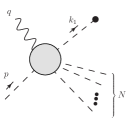
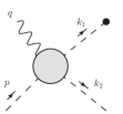
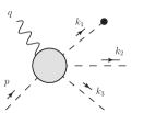
Note that at large transverse momentum, the cross section starts at order $O\left(\alpha_{s}\right)$ which is finite and well-behaved for $q_{\text{T}}>0$. The possible kinematical scenarios at $q_{\text{T}}\sim Q$ for the partonic sub cross section in the integrand on the right-hand side of Eq. (2) are sketched in Fig. 1. The dashed lines represent generic parton momenta in that all are assumed to be massless and highly non-collinear, but the exact identities of the partons are left unspecified.

The large $q_{\rm T}$ factorized cross section in Eq. (2) has power corrections suppressed by $1/q^{2}_{\text{T}}$, or $1/Q^{2}$ when $q_{\text{T}}=O\left(Q\right)$. Those corrections are not negligible in the small $q_{\text{T}}$ limit. In that limit, the cross section is best described in terms of TMD factorization, wherein the power corrections are $O(q^{2}_{\text{T}}/Q^{2})$. The first term in Eq. (2) contains contributions that would be counted as power suppressed in the $q_{\text{T}}/Q\to 0$ limit, so Eq. (2) cannot generally be inferred from the high transverse momentum behavior of TMD factorization results.

Since transverse momentum is frame dependent, characterizing its size requires some clarification. In light of the outline of regions in Sec. I, we must ask what criteria generally need to be satisfied for a transverse momentum to be considered large or small. For this, define

$$k\equiv k_{1}-q\,.$$ (4)

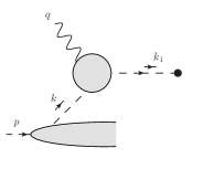
The $k$ momentum would be the target parton momentum in the small transverse momentum limit where $k^{2}\approx 0$ and the parton model $2\to 1$ subprocess $\gamma^{*}q\to q$ applies. (See Fig. 2.) Note that in Fig. 1(a), however, all the final state particles are at wide angles relative to one another, so internal propagators are off shell by order $Q^{2}$. It will also be useful to define

$$k_{X}\equiv p+q-k_{1}\,.$$ (5)

Note that in Fig. 1(b) $k_{X}^{2}=0$.

Within the blob in Fig. 1(a), two basic forms of propagator denominators may arise:

$${}\frac{1}{k^{2}+O\left(\Lambda_{\rm QCD}^{2}\right)}\,,$$ (6)

$${}\frac{1}{k^{2}+O\left(Q^{2}\right)}\,.$$ (7)

In Eq. (6), the $O\left(\Lambda_{\rm QCD}^{2}\right)$ terms are very small mass scales associated with non-perturbative physics. Equation (7) involves either the virtual photon vertex or emissions corresponding to (the wide-angle) $k_{X}$. Note that $k\cdot q\sim q\cdot p=O\left(Q^{2}\right)$. These propagator denominators illustrate the sort of power counting arguments necessary to justify the relevant factorization approximations in each region of partonic kinematics outlined in the introduction. For instance, when $|k^{2}|\approx\Lambda_{\rm QCD}^{2}$, the $k$-line is nearly on-shell and collinear to the target proton. So it should then be considered part of the proton blob, and the relevant physical picture becomes the handbag topology in Fig. 2 with $k$ now playing the role of the target parton. The $q^{2}_{\text{T}}/Q^{2}\ll 1$ approximations that lead to TMD factorization apply here. Namely, the $k^{2}$ in Eq. (7) can be neglected relative to the $O\left(Q^{2}\right)$ terms, although no small $k^{2}$ approximations are appropriate for Eq. (6).

When $|k^{2}|\approx Q^{2}$, the $O\left(\Lambda_{\rm QCD}^{2}\right)$ terms can be neglected in Eq. (6) and all of the blob in Fig. 1(a) can be calculated in pQCD with both $Q^{2}$ and $k^{2}$ acting as hard scales. Of course, it is then no longer appropriate to neglect $k^{2}$ relative to $Q^{2}$ terms in Eq. (7), so this is the large transverse momentum region 3.

Explicit diagrammatic calculations, keeping small masses, easily confirm that the coefficients of the $O\left(Q^{2}\right)$ and $O\left(\Lambda_{\rm QCD}^{2}\right)$ terms in Eqs. (6)–(7) are simple numerical factors not radically different from 1. Moreover, this generalizes to entire diagrams including propagator numerators. Thus, the ratio $|k^{2}|/Q^{2}$ is the relevant Lorentz invariant measure of the size of transverse momentum, in the sense that it should be much less than $1$ for the small transverse momentum approximations to be accurate. Calculating it in terms of $\hat{z}$, $q^{2}_{\text{T}}$ and $Q^{2}$,

$$\left|\frac{k^{2}}{Q^{2}}\right|=1-\hat{z}+\hat{z}\frac{q^{2}_{\text{T}}}{Q^{2}}\,.$$ (8)

For current fragmentation, $z$ is fixed at some value not too much smaller than $1$. (In practice it is often assumed to be between approximately $0.2$ and $0.8$.) In the integral over $\zeta$, $z<\hat{z}<1$ so

$$\frac{q^{2}_{\text{T}}}{Q^{2}}<\left|\frac{k^{2}}{Q^{2}}\right|<1-z\left(1-\frac{q^{2}_{\text{T}}}{Q^{2}}\right)\,,$$ (9)

assuming $q_{\text{T}}<Q$. So, for any $z$ in the current region, $q^{2}_{\text{T}}/Q^{2}\ll 1$ signals the onset of the TMD factorization region while $q^{2}_{\text{T}}/Q^{2}\sim 1$ signals the onset of the large transverse momentum region where fixed order pQCD is optimal. That is, $q^{2}_{\text{T}}/Q^{2}\ll 1$ implies region 1 or 2 of the introduction, while $q^{2}_{\text{T}}/Q^{2}\gtrsim 1$ implies region 3. This establishes that it is the magnitude of $\bm{q}_{\text{T}}$ specifically, defined in Eq. (1), that is most useful for assessing the transition between different regions.

Another way to estimate the boundary between large and small transverse momentum is to recall that the region 1 and 2 methods of calculating are the result of a small $q_{\text{T}}$ approximation. Thus, one may examine the effect of that approximation in specific fixed order calculations. For SIDIS at $O\left(\alpha_{s}\right)$ in the small $q^{2}_{\text{T}}/Q^{2}\to 0$ limit, the cross section is proportional to

$$d(z;\mu)\int_{x}^{1}\frac{\mathop{\mathrm{d}\mskip-0.59999mu\xi}\nolimits}{\xi}f(\xi;\mu)P(x/\xi)+f(x;\mu)\int_{z}^{1}\frac{\mathop{\mathrm{d}\mskip-0.59999mu\zeta}\nolimits}{\zeta}d(\zeta;\mu)P(z/\zeta)+2C_{F}f(x;\mu)d(z;\mu)\left(\ln\left(\frac{Q^{2}}{q^{2}_{\text{T}}}\right)-\frac{3}{2}\right)\,.$$ (10)

where the functions $P$ are lowest order splitting functions and sums over flavors are implied. (See, for example, Eq. (36) of Nadolsky et al. 1999.) The appearance of the logarithm is a consequence of approximations specific to the small $q_{\text{T}}$ limit. The actual fixed order calculation of the cross section from which this is obtained is positive everywhere. Therefore, the $q^{2}_{\text{T}}/Q^{2}\to 0$ approximation is surely inappropriate once $q^{2}_{\text{T}}$ is so large that the cross section as calculated in Eq. (10) becomes significantly negative. If the first two terms of Eq. (10) are of order unity or less, then this happens when $q_{\text{T}}\gtrsim Q$. One can use Eq. (10) to estimate where region 3 methods are definitely needed. Specific calculations in Boglione et al. 2015 show values of $q_{\text{T}}$ above which the cross section goes negative in typical calculations. For example, Fig. 1 of Boglione et al. 2015 suggests that the change of sign occurs before $q_{\text{T}}\sim Q/2$ in typical SIDIS kinematics. (This further establishes $q^{2}_{\text{T}}/Q^{2}$ as the relevant transverse momentum ratio.)

Another question is whether, for a particular combination of $x$ and $z$, the large $q_{\text{T}}$ calculation should be expected to be well-described by the $O\left(\alpha_{s}\right)$ calculation or whether higher orders are needed. For the leading $O\left(\alpha_{s}\right)$ large transverse momentum cross section, the partonic process is $2\to 2$ with all partons massless and on-shell (Fig. 1(b)), i.e., $k_{X}^{2\,\,(\alpha_{s})}=0$. For the $O\left(\alpha_{s}\right)$ calculation to be a good approximation, therefore, the ratio $k_{X}^{2}/Q^{2}$ (Fig. 1(a)) must be small enough that it does not affect the $k^{2}$ terms in Eq. (6) and Eq. (7). Considering $k^{2}/Q^{2}$ but now in terms of $k_{X}^{2}$ instead of $\hat{z}$,

$$\left|\frac{k^{2}}{Q^{2}}\right|=\frac{1}{1-\hat{x}+\hat{x}q^{2}_{\rm T}/Q^{2}}\left[\frac{q_{\rm T}^{2}}{Q^{2}}+\hat{x}\frac{k_{X}^{2}}{Q^{2}}\left(1-\frac{q^{2}_{\rm T}}{Q^{2}}\right)\right]\,.$$ (11)

So the $k^{2}$ terms in Eq. (6) and Eq. (7) are nearly independent of $k_{X}$ if $k_{X}^{2}/Q^{2}\ll 1$. Otherwise, higher orders in $\alpha_{s}$ are necessary to generate the non-zero $k_{X}^{2}$. In terms of $\hat{x}$, $\hat{z}$ and $Q^{2}$,

$$\frac{k_{X}^{2}}{Q^{2}}=\frac{(1-\hat{x})(1-\hat{z})}{\hat{x}}-\hat{z}\frac{q^{2}_{\text{T}}}{Q^{2}}\,.$$ (12)

In practice, typical $\hat{x}$ and $\hat{z}$ are largely determined by the distributions in longitudinal momentum fraction in PDFs and FFs for a particular kinematical scenario. If it turns out that they are mostly dominated by moderate values of $\hat{x}$ and $\hat{z}$, then the $k_{X}^{2}/Q^{2}\ll 1$ criterion is not difficult to satisfy for large $q_{\text{T}}\sim Q$. Then, the leading order in $\alpha_{s}$ can reasonably be expected to dominate at large transverse momentum. If, however, the typical $\hat{x}$ and $\hat{z}$ are much smaller than 1, then they force a large average $k_{X}^{2}$. This can create the situation that higher order corrections are larger relative to $O\left(\alpha_{s}\right)$ for certain regions of transverse momentum. (If there is large sensitivity to the kinematical threshold at $k_{X}^{2}\approx 0$, then this can also induce large higher order corrections.)

Note that the shape of the transverse momentum dependence can be significantly affected by the PDFs and FFs because of the correlation between $\zeta$ and $\xi$:

$$\zeta=z\left(\frac{\xi-x+xq^{2}_{\text{T}}/Q^{2}}{\xi-x-xk_{X}^{2}/Q^{2}}\right)\,.$$ (13)

Inclusive quantities are sensitive to the peak in the cross section at small $q_{\text{T}}$ (and small $k_{X}^{2}$) and thus are mainly sensitive to the region where $\zeta\approx z$. Both large $q^{2}_{\text{T}}$ and large $k_{X}^{2}$, however, push $\zeta$ to values significantly higher than $z$.

III Existing Measurements and Calculations

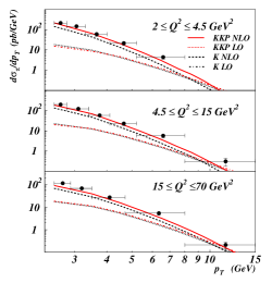
Given the discussion above, we should expect to find reasonable agreement between fixed order calculations and SIDIS measurements where $q_{\text{T}}/Q$ ratios easily exceed 1 and typical $x$ and $z$ are not such that higher orders are extremely large. This at first appears promising when considering H1 Aktas et al. 2004 kinematics , where the fixed order large-$q_{\text{T}}$ prediction from Fig. 4 of Daleo et al. 2005 (copied here in Fig. 3) gives a satisfactory description of $\pi^{0}$ production data if $O\left(\alpha_{s}^{2}\right)$ corrections are included. An obvious concern is that the order-of-magnitude higher order corrections needed might be signaling a breakdown of perturbative convergence. But as explained in Daleo et al. 2005, this behavior is most likely due simply to the particular kinematics of the H1 data. Indeed $5\times 10^{-5}\lesssim x\lesssim 5\times 10^{-3}$ for the data in Fig. 3. Also, the cross section is integrated over $z$ with

$$z=\frac{P\cdot P_{\pi}}{P\cdot q}=\frac{2xE_{p}^{2}}{Q^{2}}(E_{\pi^{0}}/E_{p})(1-\cos(\theta))$$ (14)

where $E_{p}$, $E_{\pi^{0}}$ are the energies of the proton and final state $\pi^{0}$ and $\theta$ is the polar scattering angle relative to the incoming proton direction, all defined in the H1 laboratory frame. The data are constrained to $E_{\pi^{0}}/E_{p}>0.01$ and $5^{\circ}<\theta<25^{\circ}$. Using H1 kinematics, we find that the $z$ values included in Fig. 3 can be as small as $\sim 0.001$. See section IV of Daleo et al. 2005 for more on the role of H1 cuts in producing Fig. 3. A calculation similar to Daleo et al. 2005 was performed in Kniehl et al. 2005 with similar results. The small values of $z$ are cause for caution. This is a region where a description of non-perturbative properties in terms of fracture functions (see, e.g., Trentadue and Veneziano 1994; Kotzinian et al. 2013 and also applications to SIDIS in Daleo et al. 2003; Daleo and Sassot 2003) is more appropriate.

One consequence of the small $z$ values is that $q_{\text{T}}=P_{H,\text{T}}/z$ is very large for each $P_{H,\text{T}}$ point in Fig. 3, so even the smallest transverse momenta in the plots correspond to very large transverse momenta by the criterion of Eq. (9). So it is maybe reasonable to expect that the full range of transverse momentum observable in Fig. 3 corresponds to region 3 large transverse momentum. Also, for most of the range of the integrals over $\zeta$ and $\xi$ in Eq. (2), $\hat{x}$ and $\hat{z}$ are close to zero, but with a large contribution at $\hat{x}\approx 1$. Given Eqs. (11)–(12), therefore, it is perhaps not surprising that $O\left(\alpha_{s}^{2}\right)$ calculations actually dominate since they are needed to produce the large $k_{X}^{2}/Q^{2}$.

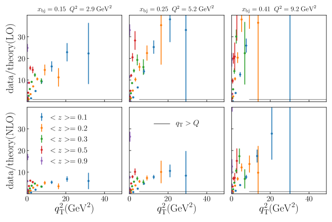
The question then, however, is whether fixed order SIDIS calculations continue to be in reasonable agreement with measurements at more moderate $x$ and $z$ and at large $q_{\text{T}}$, where the expectation is that agreement should improve, at least with the inclusion of $O\left(\alpha_{s}^{2}\right)$ corrections. Figure 4, shows that this is not the case, however. The order $O\left(\alpha_{s}\right)$ and $O\left(\alpha_{s}^{2}\right)$ curves are obtained with an analogous computer calculation as that used in Ref. Daleo et al. 2005 to generate Fig. 3, but modified to be consistent with the kinematics of the corresponding experimental data. (We have verified that the curves in Fig. 3 are reproduced.) The data are from recent COMPASS measurements for charged hadron production Aghasyan et al. 2018. Neither leading order nor next-to-leading order calculations give reasonable agreement with the measurements, even for moderate $x$, $z$ and $q_{\text{T}}>Q$, as both systematically undershoot the data, most significantly at the more moderate values of $x$ close to the valence region.

Figure 3: Fig. 4 from Daleo et al. 2005. The differential cross section was integrated over $x$, $z$ and bins of $Q$ with H1 cuts, calculated with both leading order and next-to-leading order, and compared with $\pi^{0}$ production data from Aktas et al. 2004. Here $p_{T}$ corresponds to our $P_{H,\text{T}}$ – see Eq. (1). Note the large correction from $O\left(\alpha_{s}^{2}\right)$.

Figure 4: Calculation of $O(\alpha_{s})$ and $O(\alpha_{s}^{2})$ transversely differential multiplicity using code from Daleo et al. 2005, shown as the curves labeled DDS (for Daleo-de Florian-Sassot). The bar at the bottom marks the region where $q_{\text{T}}>Q$. The PDF set used is CJNLO Accardi et al. 2016 and the FFs are from de Florian et al. 2007. Scale dependence is estimated using $\mu=\left((\zeta_{Q}Q)^{2}+(\zeta_{q_{\rm T}}q_{\rm T})^{2}\right)^{1/2}$ where the band is constructed point-by-point in $q_{\rm T}$ by taking the min and max of the cross section evaluated across the grid $\zeta_{Q}\times\zeta_{q_{\rm T}}=[1/2,1,3/2,2]\times[0,1/2,1,3/2,2]$ except $\zeta_{Q}=\zeta_{q_{\rm T}}=0$. The red band is generated with $\zeta_{Q}=1$ and $\zeta_{q_{\rm T}}=0$. A lower bound of $1$ GeV is place on $\mu$ when $Q/2$ would be less than $1$ GeV.

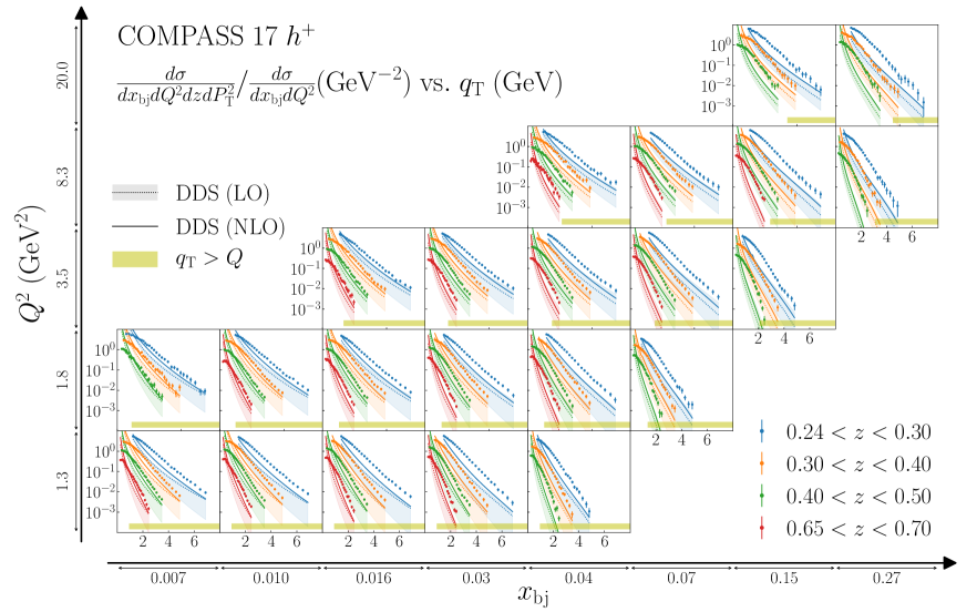
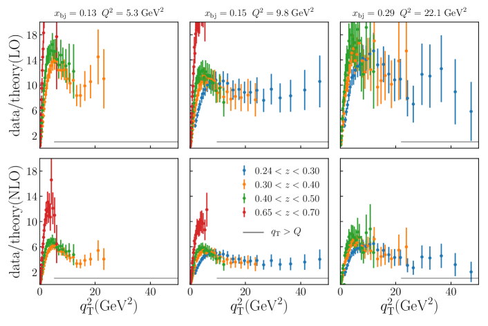
At smaller $x$ the disagreement lessens, as might be expected given the trend in Fig. 3. To highlight the valence region ($x\gtrsim 0.1$) at the larger values of $Q$, we have plotted the ratio between data and theory in Fig. 5 for three particular kinematic bins from Fig. 4. Even including the $O\left(\alpha_{s}^{2}\right)$ correction, the deviation is typically well above a factor of $2$, even for $q_{\text{T}}$ significantly larger than $Q$. In this context it is also worth considering Fig. 8 of Kniehl et al. 2005, which is for similar kinematics to Fig. 3 but for charged hadrons measured at ZEUS Derrick et al. 1996. The next-to-leading order $K$ factor is $\gtrsim 1.5$ for large transverse momentum.

Figure 5: Ratio of data to theory for several near-valence region panels in Fig. 4. The grey bar at the bottom is at $1$ on the vertical axis and marks the region where $q_{\text{T}}>Q$.

Figure 6: Calculation analogous to Fig. 4 but for $\pi^{+}$ production measurements from Ma et al. 2015.

Figure 7: Ratio calculation analogous to Fig. 5 but for $\pi^{+}$ production measurements from Ma et al. 2015.

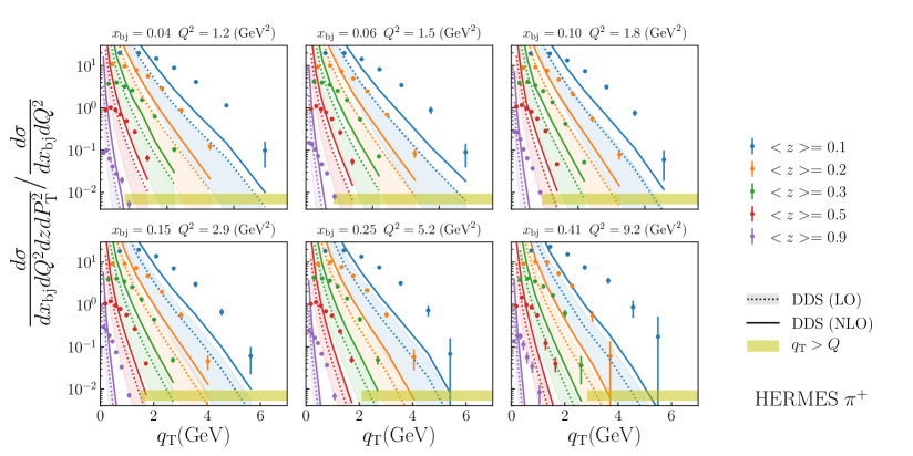
At least one other set of SIDIS data at somewhat different kinematics exhibits the same trend. This is the set of HERMES measurements of $\pi^{+}$ multiplicities Ma et al. 2015 shown in Fig. 6. Note that the kinematics very much correspond to the valence region for the target. Figure 7 shows that the failure to match the data is even more pronounced than in the COMPASS case. Even for $Q>3$ GeV and $q_{\text{T}}>Q$, the difference is nearly an order of magnitude.

IV Discussion

We have argued that there is tension between existing fixed order pQCD calculations and at least two sets of large transverse momentum measurements where those calculations should be reasonably accurate, and that this disagreement is too large to be attributable to $q_{\text{T}}$ being too small. Thus, it appears to us to be a genuine mystery that needs attention, especially for TMD phenomenology. The TMD formalism relies on approximations that apply only in the $q_{\text{T}}/Q\to 0$ limit, so it is critical to have an alternative approach to describe the transition to very large transverse momentum. If standard fixed order collinear pQCD is not adequate for this, then something new is needed.

It is worth pointing out that one encounters similar problems in Drell-Yan scattering, where a lowest order calculation with current PDF sets is easily found to undershoot the lowest available $Q$ data by very large factors. It is less clear how to interpret the disagreement here, however, since most of the existing data for lower $Q$ regions are close to the threshold region and including threshold resummation introduces extra subtleties.

The observations of this article have focused on unpolarized cross sections, but the implications extend to spin and azimuthally dependent cross sections, since the key issue is the relevance of different types of transverse momentum dependence.

There are a number of possible resolutions that deserve further investigation. An interesting one is that the hadronization mechanism is different in high-transverse- momentum SIDIS from the usual picture in terms of universal FFs. Models used in Monte Carlo event generators might be a source of ideas regarding this possibility. In the context of this possibility, it is noteworthy that much of the data for SIDIS transverse momentum dependence is describable in a Gaussian model of TMDs Anselmino et al. 2014; Signori et al. 2013. In pQCD, there are also arguments that certain higher twist correlation functions actually dominate over leading twist functions. In this picture, the $q\bar{q}$ pair that ultimately forms the final state is directly involved in the hard part Ma et al. 2015; Kang et al. 2015.

It is possible that threshold effects are important  de Florian et al. 2013; Westmark and Owens 2017. If that is the case, then there are serious implications for TMD studies, because additional non-perturbative effects beyond those associated with intrinsic transverse momentum can then be important  Collins et al. 2008. However, the largest $x$ and $z$ in Fig. 5 and Fig. 7, where the disagreement is the worst, corresponds to valence regions of $x$ and $z$, well away from kinematics where partonic kinematics are close to kinematical thresholds for most $\xi$ and $\zeta$. Furthermore, this would contradict the observation in Fig. 3 that fixed order corrections alone succeed in describing data, even for very small $x$ and $z$.

Another possibility is that FFs and/or PDFs are not well-enough constrained to handle the particular kinematical scenarios that arise at large $q_{\text{T}}$. To see that this is plausible, consider the large $q_{\text{T}}$ observable

$$\frac{\mathop{\mathrm{d}\mskip-0.59999mu\sigma}\nolimits{}}{\mathop{\mathrm{d}\mskip-0.59999muQ^{2}}\nolimits\mathop{\mathrm{d}\mskip-0.59999mux}\nolimits\mathop{\mathrm{d}\mskip-0.59999muz}\nolimits\mathop{\mathrm{d}\mskip-0.59999muq^{2}_{\text{T}}}\nolimits}\sim\int_{\xi_{\rm min}}^{1}\mathop{\mathrm{d}\mskip-0.59999mu\xi}\nolimits{}f\left(\xi\right)d\left(\zeta=z\left(1+\frac{xq^{2}_{\text{T}}}{(\xi-x)Q^{2}}\right)\right)\,,$$ (15)

where the “$\sim$” is to indicate the combination of PDF and FF that appear in fixed order pQCD calculations at large transverse momentum and lowest order. The minimum final state momentum fraction is

$$\xi_{\rm min}=x\left(1+\frac{zq^{2}_{\text{T}}}{(1-z)Q^{2}}\right)\,.$$ (16)

Note that small $\xi$ ($\xi\approx x$) tends to select the large $\zeta\gg z$ region and vice versa, and the nature of the correlation between $\zeta$ and $\xi$ changes as $q_{\text{T}}$ varies. Also, very large $q_{\text{T}}$ forces $\xi_{\rm min}$ to be large. Therefore, while the hard scattering gives a characteristic power-law shape to the large $q_{\text{T}}$ dependence, both its shape and normalization are also significantly influenced by the large $\xi$ and $\zeta$ behavior in the collinear PDFs and FFs. Note also that gluon PDFs and FFs appear in the first non-vanishing order in Eq. (15).

Contrast that with the observable,

$$\sum_{\text{Hadron Flavors}}\int z\mathop{\mathrm{d}\mskip-0.59999muz}\nolimits\mathop{\mathrm{d}\mskip-0.59999muq^{2}_{\text{T}}}\nolimits\frac{\mathop{\mathrm{d}\mskip-0.59999mu\sigma}\nolimits{}}{\mathop{\mathrm{d}\mskip-0.59999muQ^{2}}\nolimits\mathop{\mathrm{d}\mskip-0.59999mux}\nolimits\mathop{\mathrm{d}\mskip-0.59999muz}\nolimits\mathop{\mathrm{d}\mskip-0.59999muq^{2}_{\text{T}}}\nolimits}\ =\frac{\mathop{\mathrm{d}\mskip-0.59999mu\sigma}\nolimits{}}{\mathop{\mathrm{d}\mskip-0.59999muQ^{2}}\nolimits\mathop{\mathrm{d}\mskip-0.59999mux}\nolimits}\sim f\left(x\right)\,,$$ (17)

that is, the total DIS cross section; or with the $q_{\text{T}}$-integrated SIDIS cross section,

$$\int\mathop{\mathrm{d}\mskip-0.59999muq^{2}_{\text{T}}}\nolimits\frac{\mathop{\mathrm{d}\mskip-0.59999mu\sigma}\nolimits{}}{\mathop{\mathrm{d}\mskip-0.59999muQ^{2}}\nolimits\mathop{\mathrm{d}\mskip-0.59999mux}\nolimits\mathop{\mathrm{d}\mskip-0.59999muz}\nolimits\mathop{\mathrm{d}\mskip-0.59999muq^{2}_{\text{T}}}\nolimits}\ =\frac{\mathop{\mathrm{d}\mskip-0.59999mu\sigma}\nolimits{}}{\mathop{\mathrm{d}\mskip-0.59999muQ^{2}}\nolimits\mathop{\mathrm{d}\mskip-0.59999mux}\nolimits\mathop{\mathrm{d}\mskip-0.59999muz}\nolimits}\sim f\left(x\right)d\left(z\right)\,.$$ (18)

In Eq. (17), the dominant contribution at leading order is from quark PDFs only, and is evaluated only at a single value $x$. Likewise, Eq. (18) is only sensitive to the FF at $\zeta=z$. Of course, Eq. (15), Eq. (17), and Eq. (18) are all for basically the same process, but in going from Eq. (15) to Eq. (17) or Eq. (18) information is lost in the integrations and summations, and the sensitivity to the PDFs and FFs is consequently less detailed. Most typically, however, low-$Q$ fits that are aimed at constraining the valence region at lower $Q$ use observables like Eq. (17) or Eq. (18). But Eq. (15) scans through small to large values of $\xi$ and $\zeta$ as $q_{\text{T}}$ varies. The question then arises whether existing fits maintain enough information to predict Eq. (15) observables reliably. Note that it has already been suggested in the past Berger et al. 1998 to use transversely differential Drell-Yan measurements at large $q_{\text{T}}$ and including smaller $Q$ to constrain gluon distributions. An analogous possibility applies to gluon FFs at large $\zeta$ in large transverse momentum SIDIS or back-to-back hadron pair production in $e^{+}e^{-}$ annihilation. To test this, it would be informative to include the large transverse momentum behavior of lower-$Q$ but highly differential cross sections in global simultaneous fits of PDFs and FFs. It is also noteworthy that in very early calculations Halzen and Scott 1978 that gave rise to satisfactory fits in Drell-Yan scattering, the gluon and sea distributions used were much larger than modern ones. This suggests that contributions from gluon and sea PDFs and FFs at larger values of $x$ may need to be reassessed in light of the mismatches above.

We leave further investigation of all these possibilities to future work. A resolution is an important part of the goal to understand SIDIS generally in terms of an underlying partonic picture.