Integrability As Duality:
The Gauge/YBE Correspondence

Abstract

The Gauge/YBE correspondence states a surprising connection between solutions to the Yang-Baxter equation with spectral parameters and partition functions of supersymmetric quiver gauge theories. This correspondence has lead to systematic discoveries of new integrable models based on quantum-field-theory methods. We provide pedagogical introduction to the subject and summarizes many recent developments. This is a write-up of the lecture at the String-Math 2018 conference.

1 Introduction

In this review I would like to summarize some exciting recent developments in the area of applying gauge-theory ideas, and in particular Seiberg dualities, to integrable models.

In the literature there are several different (although related) characterizations of integrable models. In this lecture integrable models are defined to be the solutions of the Yang-Baxter equation [1, 2] (YBE) with spectral parameters.

Figure 1: Graphical representation of the YBE.

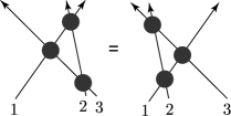
The graphical representation of YBE is given in Figure 1. Here we have three intersecting lines (often called rapidity lines) intersecting. We label them by $1,2,3$, and we associate three vector spaces $V_{1},V_{2},V_{3}$ for each line. At each crossing of the two lines (say $i$ and $j$) we associate the so-called R-matrix (see Figure 2):

$$\begin{split}R_{ij}\in\textrm{End}(V_{i}\otimes V_{j})\;.\end{split}$$ (1)

Figure 2: We associate an R-matrix at the crossing of two rapidity lines.

The YBE states that the product of three R-matrices, where the product is taken in two different orders, coincide:

$$\begin{split}&R_{23}R_{13}R_{12}=R_{12}R_{13}R_{23}\in\textrm{End}(V_{1}\otimes V_{2}\otimes V_{3})\;.\end{split}$$ (2)

Here for example $R_{12}\in\textrm{End}(V_{1}\otimes V_{2})$ is extended to a operator $R_{12}\otimes 1_{V_{3}}\in\textrm{End}(V_{1}\otimes V_{2}\otimes V_{3})$, which for simplicity we denoted by the same symbol $R_{12}$.

In this lecture we are interested in YBE with spectral parameters. This means that we have three parameters $z_{1},z_{2},z_{3}$ for the three lines $1,2,3$, and the R-matrix at the intersection of rapidity lines $i$ and $j$ depends on the associated spectral parameters $z_{i}$ and $z_{j}$:

$$\begin{split}R_{ij}=R_{ij}(z_{i},z_{j})\in\textrm{End}(V_{i}\otimes V_{j})\;.\end{split}$$ (3)

In almost all of the known integrable models, we have the property that the R-matrix depends only on the differences between the spectral parameters:

$$\begin{split}R_{ij}(z_{i},z_{j})=R_{ij}(z_{i}-z_{j})\;.\end{split}$$ (4)

This is known as the rapidity difference property of the R-matrix. This property holds for almost all the models discussed in this lecture, and in the following we will assume this property unless stated otherwise.

The YBE, now with spectral parameters, reads

$$\begin{split}&R_{23}(z_{2}-z_{3})R_{13}(z_{1}-z_{3})R_{12}(z_{1}-z_{2})\\ &\quad=R_{12}(z_{1}-z_{2})R_{13}(z_{1}-z_{3})R_{23}(z_{2}-z_{3})\in\textrm{End}(V_{1}\otimes V_{2}\otimes V_{3})\;.\end{split}$$ (5)

Once we have the YBE, then the textbook-construction of the integrable models (see e.g. [3]) ensures that transfer matrices commute with each other, and hence by expanding with respect to the spectral parameters $z$ we learn that the model has infinitely-many commuting conserved charges. This is another definition of integrability. For this reason YBE has been studied rather intensively in integrable model literature.

While there are many important questions in the field of integrable models, one of the most fundamental questions is the following:

Why integrable models exist?

This is a highly non-trivial question. For example, if one naively tries to solve the YBE (5) one finds that the equations are over-constrained in general. To see this, let us consider the situation where all the vector spaces $V_{i}$ are $N$-dimensional. Then the R-matrix, associated with the crossing of two lines, has four boundary lines and hence has $O(N^{4})$ components. By contrast, the YBE, associated with a figure with six boundary lines, has $O(N^{6})$ components. This over-counting problem is especially severe when $N$ is large, say when $N$ is infinity (namely when we consider an infinite-dimensional representation), which is indeed the case in many of the models discussed in this lecture.

It is therefore a fundamental question to understand why integrable models can exist at all. Once we have a good understanding of this one can then try to understand the pattern of existing integrable models in the literature, and moreover try to find new integrable models based on such understanding.

I myself has been fascinated by this question over the past years, and have worked mainly on two different approaches, both based on quantum-field-theory ideas.

One approach is based on the “4d Chern-Simons theory”. This approach was pursued first by Costello in 2013 [4, 5], and more recently developed further in by Costello, Witten and myself [6, 7, 8, 9, 10].

Another approach is based on supersymmetric quiver gauge theories. This approach is called the Gauge/YBE correspondence, since this correspondence claims rather direct relation between the YBE and the partition functions of gauge theories. This approach was initiated in 2012-2013 in my papers (partly in collaboration with Terashima) [11, 12, 13]. Our work is based on several previous important ideas in the literature, most notably the integrable models (known as the “master solution”) constructed by Bazhanov and Sergeev [14, 15]. By now I have succeeded in reproducing their construction from scratch, and generalized the master solution in a number of different directions, based on quantum-field-theory techniques.

In the rest of this lecture I will discuss the second approach to this subject.

2 Basic Ingredients

While there are many technical complications needed in the actual discussions of the subject, the fundamental ideas behind the Gauge/YBE correspondence are rather simple, and can be listed as follows:

• a statistical lattice as a quiver diagram

• supersymmetric localization

• Seiberg(-like) duality

2.1 Statistical Lattice as Quiver Diagram

2.1.1 Statistical Mechanical Model

In textbook presentation of statistical mechanics, one starts with a statistical lattice, such as the one shown in Figure 3. Let us denote the set of vertices by $V$, and edges by $E$.

Figure 3: Statistical lattice where a statistical-mechanical model is defined. We can also regard this as a quiver diagram, a defining data for the quiver gauge theory.

In the statistical-mechanical model, the dynamical degrees of freedom of the theory, namely ‘spins’, are placed at the vertices of the lattice: $s_{v}$ at vertex $v\in V$. The spins here can take values in any set and can be discrete or continuous. For example $s_{v}=\pm 1$ for the Ising model. In this lecture we will encounter more complicated examples where $s_{v}$ takes values in e.g. $(\mathbb{R}\times\mathbb{Z}_{r})^{N-1}$ for integers $r,N$ (with $N>1$) [13]: in this example we $s_{v}$ has multiplet components, and has both discrete and continuous components.

The partition function of the statistical-mechanical model is defined as

$$Z:=\sumint\left(\prod_{v\in V}ds_{v}\right)e^{-\mathcal{E}\left(\{s_{v}\}_{v\in V}\right)}\;.$$ (6)

Here the symbol $\sumint\prod_{v\in V}ds_{v}$ denotes the summation over the spin configuration $\{s_{v}\}_{v\in V}$. When $s_{v}$ has only discrete (continuous) components this should be understood as $\sum_{\{s_{v}\}_{v\in V}}$ ($\int\prod_{v\in V}ds_{v}$), and in general we sum (integrate) over the discrete (continuous) part of the spins.

Inside the integrand of (6) we have the so-called Boltzmann weight $\mathcal{E}\left(\{s_{v}\}\right)$, a function of spins given as a sum of contributions from edges and vertices:

$$\begin{split}\mathcal{E}\left(\{s_{v}\}_{v\in V}\right)=\sum_{v\in V}\mathcal{E}^{v}(s_{v})+\sum_{e\in E}\mathcal{E}^{e}\left(\{s_{v}\}_{v\in e}\right)\;,\end{split}$$ (7)

where $v\in e$ means that the vertex $v$ is one of the two endpoints of the edge $e$. The function $\mathcal{E}^{e}$ specifies the nearest-neighbor interaction of the spins, while $\mathcal{E}^{v}(s_{v})$ specifies the local interaction at the vertex (such as the magnetic field dependence in the Ising model, or the self-interaction between different components of the spin).

2.1.2 Quiver Gauge Theory

Instead of starting with a statistical-mechanical model, we would like to start with a quantum field theory defined from the statistical lattice.

In high energy physics there are several ideas along these lines. For example, the lattice gauge theory indeed is defined on a discrete lattice. We here instead discuss the concept of quiver gauge theory.

In quiver gauge theory we regard the statistical lattice as the “quiver diagram”, which specifies the gauge/matter content of the theory. Namely,

• For each vertex $v\in V$ we associate a gauge field $A_{v}$ valued in the gauge group $G_{v}$. This means that the total gauge group of the theory is

  $$\begin{split}G_{\rm total}=\prod_{v\in V}G_{v}\;.\end{split}$$ (8)

• For each edge $e\in E$ with two endpoints given by $v,v^{\prime}\in V$ we associate a matter field $\phi_{e}$ which transforms non-trivially under some representation of $G_{v}\times G_{v^{\prime}}$, but otherwise trivially under $G_{v^{\prime\prime}}$ for $v^{\prime\prime}\neq v,v^{\prime}$.

In this discussion, the statistical lattice is simply a mnemonic for the gauge/matter content of the theory, and does not have any direct relation with the actual spacetime where the quantum field theory is defined.

The partition function of this quantum field theory is defined by the path-integral:

$$\begin{split}Z=\int\prod_{v}\mathcal{D}A_{v}\prod_{e}\mathcal{D}\phi_{e}\,\,e^{-L\left(\{A_{v}\}_{v\in V},\{\phi_{e}\}_{e\in E}\right)}\;,\end{split}$$ (9)

where $\mathcal{D}A_{v}$ and $\mathcal{D}\phi_{e}$ denote the path-integral measures for the quantum fields $A_{v}$ and $\phi_{e}$.

The integrand, namely the Lagrangian $L$, is a functional of the field configurations $\{A_{v}\}_{v\in V},\{\phi_{e}\}_{e\in E}$, and is given by

$$\begin{split}L\left(\{A_{v}\}_{v\in V},\{\phi_{e}\}_{e\in E}\right)=\sum_{v\in V}L^{v}\left(A_{v}\right)+\sum_{e\in E}L^{e}\left(\{A_{v}\}_{v\in e},\phi_{e}\right)\;.\end{split}$$ (10)

Here the term $L^{v}$ is the kinetic term for the gauge field $A_{v}$, and the term $L^{e}$ is the Lagrangian for the field $\phi_{e}$, which couples non-trivially to the gauge fields $\{A_{v}\}_{v\in e}$.

2.1.3 Comparison

There is a striking parallel between the two stories above, between statistical-mechanical models and quiver gauge theories. For example, the role of the spins $s_{v}$ are played by the gauge fields $A_{v}$, and in the partition functions (6) and (7) are replaced by (9) and (10), respectively.

Encouraged by this parallel, one can try to construct the statistical-mechanical model from quantum field theory.

There are still important differences between the two stories, however.

• In statistical mechanics all the degrees of freedom (namely spins $s_{v}$) live at the vertices. Quiver gauge theory, by contrast, has matter fields $\phi_{e}$ located at the edges, in addition to the gauge fields $A_{v}$ located at the vertices. In other words, we have a non-standard statistical-mechanical model where we have degrees of freedom both at the edges and the vertices.

• In quiver gauge theory the partition function (9) is defined by the path integral, and does not necessarily fit with the more conventional discussion of statistical-mechanical models (6), where the partition function is defined by a finite integral/sum.

In the next subsection we shall explain how these differences are removed with the help of supersymmetry.

2.2 Supersymmetric Localization

The second ingredient of the Gauge/YBE correspondence is supersymmetric localization.

Suppose that we supersymmetrize our quiver gauge theory. The details of how this works depends of course on the dimensionality and the number of supersymmetries.

While the story below will work in general, let us for concreteness consider the case of four-dimensional quiver gauge theory with ${\cal N}=1$ supersymmetry (namely four supercharges). Then we have

• For each vertex $v\in V$ we associate an ${\cal N}=1$ vector multiplet $V_{v}=(A_{v},\lambda_{v},F_{v})$, whose on-shell degrees of freedom contains a gauge field $A_{v}$, a gaugino $\lambda_{v}$, and an auxiliary field $F_{v}$, all in the adjoint representation of the gauge group $G_{v}$.

• For each edge $e\in E$ with two endpoints given by $v,v^{\prime}\in V$ we associate an ${\cal N}=1$ chiral multiplet $\Phi_{e}=(\phi_{e},\psi_{e},D_{e})$ in a non-trivial representation of $G_{v}\times G_{v^{\prime}}$: this multiplet contains a complex scalar $\phi_{e}$, a fermion $\psi_{e}$, and an auxiliary field $D_{e}$.

The definition of the partition function is of course then supersymmetrized:

$$\begin{split}Z&=\int\prod_{v}\mathcal{D}V_{v}\prod_{e}\mathcal{D}\Phi_{e}\,\,e^{-\mathcal{L}\left(\{V_{v}\}_{v\in V},\{\Phi_{e}\}_{e\in E}\right)}\;.\end{split}$$ (11)

where we denoted the supersymmetrized path-integral measure as

$$\begin{split}\mathcal{D}V_{v}=\mathcal{D}A_{v}\mathcal{D}\lambda_{v}\mathcal{D}F_{v}\;,\quad\mathcal{D}\Phi_{e}=\mathcal{D}\phi_{e}\mathcal{D}\psi_{e}\mathcal{D}D_{e}\;.\end{split}$$ (12)

Then partition function (11), when considered in the flat spacetime, is in general a divergent quantity. We can however regularize the IR divergence by placing the theory on a certain compact manifold $M$, and after suitably regularizing the UV divergence we can define a well-defined partition function $Z[M]$; we use the same formula (11) but now everything is defined on $M$.

Now the supersymmetric partition function states that we can compute the partition function $Z[M]$, which is a priori defined as an infinite-dimensional path-integral, reduces to a finite-dimensional integral/sum:

$$\begin{split}Z&=\sumint\prod_{v\in V}d\sigma_{v}\,\,e^{-\mathcal{L}(\sigma_{v})}\;.\end{split}$$ (13)

In (13) $\sigma_{v}$ is a finite-dimensional variable associated at the vertex $v\in V$ (namely associated with the gauge group $G_{v}$), and as we will see can be continuous or both continuous and discrete variables depending on the choice of the manifold $M$. In the examples below $\sigma_{v}$ arises from the holonomies of the gauge field along the non-trivial cycles of $M$. Note that there is no integral/sum variable associated with the edges of the graph, i.e. the matter fields $\phi_{e}$ vanish at the saddle point locus. While this is not guaranteed in general supersymmetric localization, this is indeed the case in all the examples we study in this lecture, and in any case in the following we will assume this.

Finally, the integrand is $\mathcal{L}(\sigma_{v})$ takes the form

$$\begin{split}\mathcal{L}\left(\{\sigma_{v}\}_{v\in V}\right)=\sum_{v\in V}\mathcal{L}^{v}\left(\sigma_{v}\right)+\sum_{e\in E}\mathcal{L}^{e}\left(\{\sigma_{v}\}_{v\in e}\right)\;.\end{split}$$ (14)

Here $\mathcal{L}^{v}$ ($\mathcal{L}^{e}$) denotes the classical plus one-loop contributions from the gauge fields (matter fields). This formula should be compared with the Boltzmann weight for the statistical-mechanical model (7).

2.2.1 Some More Details

The discussion of the quiver gauge theory above is rather general, and for practical purposes one needs to specify the theory more in detail.

First, we need to specify the spacetime dimension $D$ for the the quiver gauge theories are defined—for example, the gauge field $A_{v}$ introduced above is $A_{v}^{\mu}(x)$, where $\mu$ runs from $0,\ldots,D-1$, and $x$ is a point of the $D$-dimensional geometry, such as $\mathbb{R}^{1,D-1}$. In practice we will consider the case of $D=4,3,2,1$.

Second, we did not specify the representation of the matter field $\phi_{e}$ under the symmetry $G_{v}\times G_{v^{\prime}}$ (where two endpoints of $e$ are denoted by $v,v^{\prime}\in e$). In this lecture we choose the gauge group $G_{v}$ to be an $SU(N_{v})$ gauge group (with rank specified by an integer $N_{v}$), and the matter field to be in the so-called bifundamental representation, namely in the representation $(\square,\overline{\square})$ under $G_{v}\times G_{v^{\prime}}$. We then need to distinguish the two endpoints, and hence combinatorially we now need to consider oriented edges, as in Figure 4.

Figure 4: Statistical lattice where a statistical-mechanical model is defined.

That we need to specify the orientation of the arrow means that the our quiver gauge theory is now chiral. This is indeed the case for almost all the theories we discuss in this paper (except in section 5). In terms of statistical-mechanical models, this chirality means that the Boltzmann weight for an edge $e$ is asymmetric with respect to the exchange of the endpoints of the edge:

$$\mathcal{E}^{e}(s_{v},s_{v^{\prime}})\neq\mathcal{E}^{e}(s_{v^{\prime}},s_{v})\;.$$ (15)

In Figure 4 we have chosen the orientation of the edges such that for each face of the lattice (e.g. a square in Figure 4) all the edges around the face are all in the same direction, either all clockwise or all counterclockwise. This also means that we have a corresponding gauge-invariant product of the bifundamentals around the face, which we can use as a term in the superpotential:

$$\begin{split}W=\textrm{Tr}\left[\overset{\curvearrowright}{\prod}_{e\in\textrm{ clockwise face}}\Phi_{e}\right]-\textrm{Tr}\left[\overset{\curvearrowleft}{\prod}_{e\in\textrm{ counterclockwise face}}\Phi_{e}\right]\;.\end{split}$$ (16)

This will be our general rule in the rest of this lecture.

Finally, we have not the boundary condition for the statistical-mechanical model: this can be say either periodic boundary condition or fixed boundary condition. In quiver gauge theory language, the difference is whether to consider the quiver diagram on the torus [33, 34] or on a disc [38, 17]. For the latter case we have external quiver vertices, whose associated symmetry we regard as a non-dynamical flavor symmetry.

2.3 Seiberg(-like) Duality

The final ingredient is the Seiberg(-like) duality. This is represented graphically in Figure 5.

Figure 5: Graphical representation of the Seiberg(-like) duality for quiver gauge theories. The same picture can also represent a quiver mutation in cluster algebras, or the star–star relation in integrable models.

The two quivers in Figure 5 can be regarded as the defining data for the quiver gauge theory. As for the vertices, the circles represent the gauge symmetry, where as the squares represent the flavor symmetry. Here and in the following we choose symmetry group to be $G_{v}=\mathrm{SU}(N)$ at all the vertices $v\in V$, either gauge or flavor, and fix this integer $N$ throughout.

The theory is known as the $\mathrm{SU}(N)$ SQCD with $2N$ flavors (since two arrows comes into the middle circle vertex, and two arrows out). The non-Abelian part of the flavor symmetry is $\mathrm{SU}(2N)_{L}\times\mathrm{SU}(2N)_{R}$, which in this case is broken to its subgroup $\mathrm{SU}(N)^{4}$. Such a breaking is caused by the presence of “mesons”, which are represented as two arrow connecting a square to another, and hence transforms as bifundamental representation with respect to the $\mathrm{SU}(N)\times\mathrm{SU}(N)\subset\mathrm{SU}(N)^{4}$ flavor symmetry.

For the case of 4d ${\cal N}=1$ theories, the duality between the two theories, which holds in the long distance limit, is then the famous Seiberg duality [39], where the case of $N_{f}=2N$ flavors is right in the middle of the conformal window. Note that following the previous rule (16) we here include a cubic superpotential term for each triangle in Figure 5, and such a superpotential term (meson–quark–quark superpotential term) is needed for the Seiberg duality.

There are similar versions in 3d ${\cal N}=2$ [40] and 2d ${\cal N}=(2,2)$ [41, 42], and we will collectively refer to all of them as Seiberg-like dualities, or simply Seiberg dualities.

For mathematically-inclined readers Figure 5 can be thought of as a special example of the quiver mutation [43, 44]. We will not really take advantage of this interpretation, partly because Seiberg duality in four dimensions corresponds only to a special subset of the more general quiver mutation (in two dimensions there is a closer relation between Seiberg duality and quiver mutation [42], a fact which we will comment again later in this paper).

It is fair to say that these two interpretations mentioned above of Figure 5, in terms of Seiberg duality and quiver mutation, are well-known in the literature.

What is less known is that the same graph has yet another interpretation in statistical mechanics—the star–star relation (SSR) [45, 46].

The motivation for SSR in the context of integrable models is that SSR implies YBE, and hence once we solve the SSR we automatically obtain an integrable model. This fact has far-reaching implications, and is one of the cornerstones of the Gauge/YBE correspondence.

We can now put together all the ingredients discussed in this section.

We can start with Figure 5, which we can regard as the quiver diagram and associate quiver gauge theories. Thanks to Seiberg duality, we know that the two theories are dual, and hence their partition functions coincide in the IR. Since Figure 5 is simultaneously the SSR, we have solved the SSR by computing the supersymmetric partition function of the quiver gauge theories: that such a partition function has statistical-mechanical interpretation was explained in section 2.1.2 and 2.2. This means that we have solved SSR, and hence have solved the YBE!

3 YBE as Duality

While the explanation given in the previous section is enough to understand minimally how we obtain integrable models, it is instructive to look into the construction in more detail. Interestingly, almost all the ingredients in integrable models have counterparts in quiver gauge theories, and we find a step-by-step parallel.

3.1 Theory for R-matrix

For our later purposes it is useful to represent the SSR in Figure 5 more symmetrically by adding half-arrows [19]. This is shown in Figure 6, where half-arrows are shown as dotted lines.

The rule is that when we have a full arrow in one direction and a half arrow in the opposite direction, we can then cancel them into a half-arrow (as in Figure 6). After this manipulation we obtain an expression as in the bottom of Figure 6.

Figure 6: More symmetric representation of the SSR. Here a dotted line is a half-line, which when combined with a full-line in an opposite orientation creates a half-line.

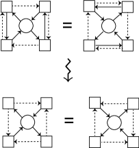
One should note that there is no such thing as a half-matter (say a half-chiral multiplet) in quiver gauge theories. Such a half-line, however, helps to explain the integrability structure in a more symmetric and unified manner. Note that in our following discussions half-arrows always connect flavor symmetry gauge groups (squares), and hence non-dynamical. At the level of the supersymmetric partition functions the only change from the full matter is that we take a square root of the corresponding classical/one-loop contribution. In any case, whenever we discuss dualities among quiver gauge theories we can always cancels the half arrows so that the duality can be stated in terms of full arrows only (we will see this in Figure 10.).

The claim now is that the quivers in Figure 6 should be regarded as the quiver for the R-matrix (Figure 7):

Figure 7: We associate he quiver in the Figure 6 to the R-matrix of the integrable model: the R-matrix is now promoted to a “theory” $\mathcal{T}[R]$!

In other words, the theory $\mathcal{T}[R]$ specified by the quiver is the “gauge-theory uplift” of the R-matrix. To better understand this statement we need to discuss the YBE for this R-matrix.

3.2 Gluing as Gauging

In order to discuss YBE we need to combine the three R-matrices. Let us see how this works at the level of the quiver diagram, and hence of the quiver gauge theory.

Let us first glue two R-matrices. In the left figure of Figure 8 we need to cancel the half-lines in the opposite directions, to obtain the quiver as in the right of Figure 8.

Figure 8: Gluing of two R-matrices.

We can next combine three R-matrices as in Figure 9. We again cancel the two half-arrows in opposite directions; in addition we combine the two half-arrows into a one full arrow, when the two are in the same direction.

Moreover the vertex in the center of the figure at the contact point of three rhombi is now turned into a circle, namely the corresponding $\mathrm{SU}(N)$ symmetry is gauged. In general, the rule is that an internal vertex is gauged, whereas an external vertex is not gauged. In this sense we are gluing the three copies of the theory $\mathcal{T}[R]$ by appropriate gauging.

Figure 9: We combine the three R-matrices. Depending on the orientations the two half-arrows either cancels or combines into a full arrow. The vertex in the center, now an internal vertex, is promoted to the gauge symmetry.

Note that the idea of “gluing the theories by gauging” is has appeared in many physics problems in the past, and has been popular after the discovery of the so-called class $S$ theories [48]. Indeed, many of our discussions here is parallel to the discussion there. For example the role of the trinion theory (the so-called $T_{N}$ theory) there is played by our R-matrix theory $\mathcal{T}[R]$. The choice of the Riemann surface obtained by gluing trinion, is here played either by the choice of the toric diagram for quivers on the torus [33, 34] and the choice of the decorated permutation [17, 38] for quivers on the disc.

3.3 Yang-Baxter Duality

We are now ready to discus the YBE. Since the combination of the three R-matrices shown in Figure 9 is the left hand side of the YBE, we can do the same for the right hand side and immediately write down the quiver counterpart of the YBE, to obtain Figure 10(b). We can again add half-arrows as in Figure 10(c), and then cancel/combine the half-arrows, to obtain Figure 10(d).

Figure 10: The quiver counterpart of the YBE. After combining the three R-matrices as in (a)(b). After adding the half-arrows for the external global symmetries as in (c) and canceling/combining the half-arrows on both sides of the identity, we obtain an equality in (d). The gauge theory interpretation of this is that the two quivers in (c) are dual, namely they flow to the same IR fixed point.

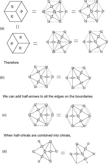
The final equality in Figure 10(d) contains a precise gauge theory statement. Namely, the quiver gauge theories, described by two quivers in Figure 10(d), are dual, namely they flow to the same IR fixed point. Since this duality is the precise counterpart of the YBE, let us call this duality the Yang-Baxter duality.

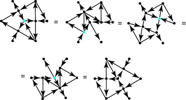
Of course, the question is then if this duality holds. Fortunately for us, we can show that the Yang-Baxter duality follows by repeated use of the Seiberg duality, as shown in Figure 11.

Of course, this is essentially the explanation that the SSR implies the YBE, a fact which was known already in the old literature of integrable models [45, 46]. What is new here is that we are now discussing the quiver gauge theories attached to the same figures, and as we will see this understanding is remarkably powerful in constructing new integrable models.

Figure 11: The Yang-Baxter duality follows by repeated use of the Seiberg duality. In this figure the blue vertices denote the gauge groups where we perform the Seiberg duality (quiver mutation) in the next step.

4 Spectral Parameter as R-charge

4.1 Zig-Zag Paths and R-charge

There is still one missing ingredient in our discussion so far: the spectral parameter in integrable models. As commented before, this parameter is essential in obtaining an infinitely-many conserved charges.

In the Gauge/YBE correspondence, the gauge-theory counterpart of the spectral parameter in integrable models is the R-charge. Simply put, in both cases the parameters are associated with the so-called “zig-zag paths”.

Since a picture is worth a thousand words, the best way to explain the zig-zag path is simply to show Figure 12, and I hope that the rule is self-explanatory. In Figure 12 the zig-zag paths (colored red) is a path coming in from infinity and eventually goes off to infinity. They intersect precisely once for each edge of the original quiver diagram (colored black).

Figure 12: Zig-zag paths, represented by red lines. We have shown the zig-zag paths as dotted or undotted lines, to make it easier to distinguish between different lines. We can recover the original quiver diagram from the zig-zag paths only. For this reason the zig-zag paths contain the same data as the original quiver diagram.

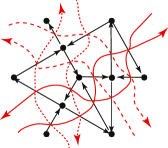
The zig-zag paths give a nice parametrizations of the R-charges. Let us label the zig-zag paths by $i=1,2,\ldots$, and let us associate an angle $\theta_{i}$ for each path. Since $\theta_{i}$ is an angle, we have the identification $\theta_{i}\sim\theta_{i}+2\pi$. Suppose that one wants to know the R-charge of the matter multiplet. In quiver gauge theory such a matter is located at an edge of the quiver diagram, where two zig-zag paths, say $i$ and $j$, cross. Then the R-charge of the matter multiplet is given by $\theta_{ij}/\pi$, where $\theta_{ij}$ is the relative angle between $\theta_{i}$ and $\theta_{j}$. Readers are referred to [54, 11, 17] for more details of this parametrization. Note that the condition that the sum of R-charges is $2$ is analogous to the statement that the sum of the R-charges is $2\pi$, and the point is that one can promote this analogy into a precise correspondence.

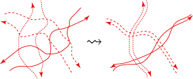
Apart from parametrizing R-charges, the zig-zag paths contain exactly the same data as the original quiver diagram. In fact, by looking at Figure 12 one can convince oneself that we can recover the original quiver diagram from the zig-zag paths only. For this reason, we are free to disregard the quiver diagram and keep only the zig-zag paths. If we do this for the left figure of Figure 13 and deform the paths (while keeping the topology of the graph), we arrive at the right figure of Figure 13, which is very similar to the picture for the YBE (recall Figure 1). We can also represent the SSR and the YBE in terms of the zig-zag paths, as in Figures 14 and 15. The previous statement that SSR implies YBE is now an exercise in graphical calculus: we need to show the equality of the zig-zag paths in Figure 15 by using the moves in Figure 14. I would like to invite the readers to check this statement directly to one’s satisfaction.

Figure 13: We can disregard the quiver diagram from Figure 12, to obtain a set of zig-zag paths as in this figure. By appropriately deforming the paths (while keeping the topology of the graph) we arrive at the picture on the right, which is very similar to the picture for the YBE (recall Figure 1).

Figure 14: Graphical representation of SSR, now in terms of the zig-zag paths. SSR is here represented by a move involving four zig-zag paths.

Figure 15: YBE as implied by SSR, now reformulated in terms of zig-zag paths. The resulting picture has doubled rapidity lines running parallel in the opposite directions, and has ‘twists’ in several places.

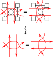
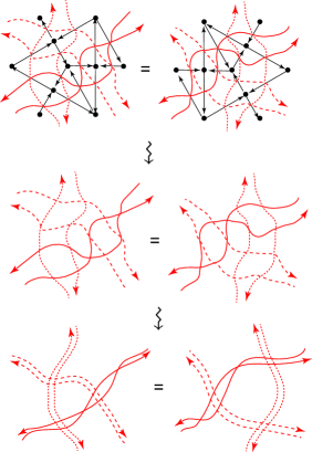
There are still some differences from Figure 1. First, the role of a single rapidity line is now played by a pair of zig-zag paths which run parallel with each other in the opposite direction. Second, in the bottom figure of Figure 15 such a pair of zig-zag paths are twisted in four locations. One can therefore say what we obtain here is a “doubled twisted” YBE.

The existence of the ‘twist’ of course does not mean that we have failed to solve the YBE. Recall that whole construction arises from solving the YBE as in Figure 10, and we have already seen in Figure 11 that the Seiberg-like duality (solution to SSR) solves the YBE on the nose. The ‘twist’ in Figure 15 arises only when we try to eliminate the half-arrows and represent everything in terms of zig-zag paths.

The origin of this ‘twist’ can be traced back to the existence of the mesons in the Seiberg duality in Figure 6. It is interesting to see that the integrable model experts, at least in their own context, knew that mesons are needed for a proper discussion of SSR (Seiberg-like duality), years before the discovery of Seiberg duality in 1994.

4.2 Zig-Zag Paths from String Theory

We have so far introduced the zig-zag paths as purely combinatorial objects. This is often the case in the literature, either in integrable models or in quiver gauge theories. Fortunately we can do better in string theory and identify the zig-zag paths as the “shape of the branes”.

Let us discuss this point briefly for the case of 4d $\mathcal{N}=1$ quiver gauge theories, following the author’s Master’s thesis [36].

Let us consider type IIB string theory on $\mathbb{R}^{3,1}_{0123}\times(\mathbb{C}^{\times})^{2}_{4567}\times\mathbb{C}_{89}$. $N$ D5-brane spread in $012357$-directions, with $57$ directions compactified (namely gives $T^{2}$), realizing $\mathrm{SU}(N)$ gauge groups. We in addition have one NS5-brane, filling the $0123$ directions as well as a holomorphic curve $\Sigma(x,y)=0$ (with $x=e^{x_{4}+ix_{5}},y=e^{x_{6}+ix_{7}}$) inside $(\mathbb{C}^{\times})^{2}$ ($4567$-directions), see Table 1.

Table 1: The type IIB configuration realizing 4d $\mathcal{N}=1$ quiver gauge theories.

	0	1	2	3	4	5	6	7	8	9
D5	$\circ$	$\circ$	$\circ$	$\circ$		$\circ$		$\circ$
NS5	$\circ$	$\circ$	$\circ$	$\circ$	$\Sigma$ (2-dim surface)

The NS5-brane and D5-brane intersect along paths (1-cycles) on the $57$-torus, and these paths are identified with the zig-zag paths introduced before. The zig-zag paths divide the torus into various regions, realizing the quiver structure of the gauge group (see [36] for details). The Seiberg duality (as in Figure 14) can be understood as a reordering of the five-branes reminiscent of the Hanany–Witten transition [68]. Note that in this brane setup the R-symmetry (which we associate with the spectral parameters) can be identified with the rotation symmetry in the transverse $89$-plane.

Other than providing a natural explanation of the zig-zag paths, the five-brane configuration could be a useful starting point for exploring other approaches to integrable models, for example with the “4d Chern-Simons” approach mentioned in introduction. This requires further study, see e.g. [18, 69, 70, 71].

5 $\mathrm{SU}(2)$ and Star-Triangle Relation

Let us next comment on the special case where the gauge groups at the quiver vertex is $\mathrm{SU}(2)$ (as oppose to $\mathrm{SU}(N)$ with $N\geq 2$). This is special since in this case there is no distinction between the fundamental representation and the anti-fundamental representation. Correspondingly the theory is non-chiral, and there is no need to specify the orientation of the edges of the quiver diagram, and of the zig-zag paths.

Of course, everything we said so far applies to the special case of $\mathrm{SU}(2)$. The notable difference for the $\mathrm{SU}(2)$ case is that the Seiberg duality as represented in Figure 6 follows in turn from another Seiberg duality, as shown in Figure 16.

Figure 16: For $\mathrm{SU}(2)$ gauge groups we can consider the duality for the star-triangle relation. This in turn implies the SSR, and hence is more fundamental as a duality. In terms of zig-zag paths this represents the reshuffling of the positions of the three zig-zag paths. Note that the zig-zag paths are here not oriented, and the theory is non-chiral.

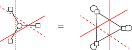
In the left figure of Figure 16 the gauge vertex in the middle has three arrows coming in, and hence we have $N_{f}=3$ (namely $6$ doublets), with $\mathrm{SU}(6)$ symmetry broken into $\mathrm{SU}(2)^{3}$. This theory is known (again by the Seiberg duality [39]) to a non-gauge theory with $\binom{6}{2}=15$ mesons. In the right figure of Figure 16, $12$ of these mesons are shown as edges connecting two flavor $\mathrm{SU}(2)$ symmetries, where the remaining $3$ mesons are in the adjoint representation with respect to the one of the $\mathrm{SU}(2)$ flavor symmetries.

Figure 16 is known in integrable model literature as the star-triangle relation (STR), one of the expressions for the YBE [3]. We therefore conclude that the duality in Figure 16 generates a solution to the STR [16].

In terms of zig-zag paths Figure 16 means that we can move the relative positions of any three zig-zag paths. This implies the SSR and then in turn the YBE (representation of the Yang-Baxter duality) for our R-matrix; in terms of zig-zag paths both are represented as certain moves of the paths (see Figures 14 and 15), and these easily follow since we can change the position of any three paths, and hence of any paths.

Summarizing, we find

STR: ($$\mathrm{SU}(2)$$ Seiberg duality with ( doublets))

SSR: ( Seiberg duality with ( doublets))

YBE: (Yang-Baxter duality)  .

(17)

6 New Integrable Models

Having explained the general theory, let us now turn to the question: which concrete integrable model arises from the general construction of the previous section?

6.1 General Lessons

Before answering this question, let us first summarize our overall logic as in Figure 17.

Figure 17: The Yang-Baxter duality “uplifts” integrable models into gauge theories and unifies many integrable models which are unrelated otherwise. Namely, starting with a single duality we can compute various different supersymmetric partition functions and obtain many different dualities. In addition we can change the gauge theory side by for example dimensionally reducing the theory. Such a gauge theory operation, as long as it preserves the duality, has counterparts in the integrable model side.

In a typical discussion of integrable models we choose a specific integrable model (a solution of YBE), for example the one denoted as YBE₁ in Figure 17. Rather, here we are interested in the underlying Yang-Baxter duality (denoted Yang-Baxter duality_a in Figure 17): this can be thought of as a “gauge-theory uplift” of YBE₁, and conversely YBE₁ is obtained by computing a supersymmetric partition function $Z[M_{1}]$ on a manifold $M_{1}$.

Once we have the Yang-Baxter duality we can systematically construct a variety of integrable models, by computing a different supersymmetric partition function (for example $Z[N_{1}]$ in Figure 17). In this sense the Yang-Baxter duality unifies many different integrable models, which as integrable models look completely unrelated.

Once we establish the correspondence we can further generalize the setup by applying various operations on the field theory side. For example, we can dimensionally reduce the theory along some directions of the compactification manifold, or we can integrate out some matters by giving mass. As long as these operations preserve the duality, one should land on another version of the Yang-Baxter duality, which we called Yang-Baxter duality_b in Figure 17.

The relation between two different versions of the Yang-Baxter duality (Yang-Baxter duality_a and Yang-Baxter duality_b in Figure 17) on the field theory side can now be translated into the integrable model side. For example, suppose that we dimensionally reduced the field theory along a circle, and suppose that the manifold $M_{1}$ contains a circle as a fiber, with the based manifold $M_{2}$. We then expect that the partition function on $M_{1}$ should reduce to the partition function on $M_{2}$, and this process looks like a degeneration of the associated integrable models.

We can repeat the procedure above, and obtain a whole zoo of integrable models.

6.2 New Integrable Models

Let us now make the setup more concrete. We first need to specify which spacetime dimension we are in (in all the dimensions we consider a supersymmetric theory with four supercharges). We then need to choose a supersymmetric partition function, which we represent by the choice of the manifold $M$.

Once we fix the choice of the supersymmetric partition function, the resulting partition function is in general a function of the certain data of the manifold $M$. For example, for $S^{1}\times S^{3}$ the partition function depends on two continuous parameter ${\mathsf{p}}$ and ${\mathsf{q}}$, which parametrizes the complex structure on $S^{1}\times S^{3}$ [73, 74]. The partition function is (up to the overall supersymmetric Casimir energy contribution) the same as the superconformal index of [75], where the parameters ${\mathsf{p}},{\mathsf{q}}$ are the fugacities in the definitions of the index.

Figure 18: A zoo of supersymmetric partition functions (and of associated integrable models). The arrows represents a dimensional reduction into one dimension lower. The case of $S^{1}\times S^{3}/\mathbb{Z}_{r}$ in four dimensions, whose associated integrable model is the super-master solution of YBE, is particularly general, and contains many other known solutions in the literature.

The actual integrable model has been discussed in many papers in the literature. While it is difficult to precisely summarize the rich literature, it might be useful for readers to loosely classify the literature into: 4d $\mathcal{N}=1$ on $S^{1}\times S^{3}$ [14, 15, 16, 11, 12, 17, 24, 23, 28], on $S^{1}\times S^{3}/\mathbb{Z}_{r}$ [13, 25, 21, 22, 29], 3d $\mathcal{N}=2$ on $S^{1}\times S^{2}$ [18, 20, 27, 31], on $S^{3}$ [76, 11, 12] and $S^{3}/\mathbb{Z}_{r}$ [22], 2d $\mathcal{N}=(2,2)$ on $S^{2}$ [26], on $T^{2}$ [18, 19, 30], and 1d $\mathcal{N}=4$ on $S^{1}$ [26].

Rather than listing all the solutions, let us here comment on some notable features of the resulting integrable models.

The Boltzmann weights are written in terms of some special functions. For example,

• For 4d $S^{1}\times S^{3}/\mathbb{Z}_{r}$ we find the elliptic gamma function (as noticed first in [77])

  $$\begin{split}\Gamma(x;{\mathsf{p}},{\mathsf{q}})=\prod_{j,k\geq 0}\frac{1-x^{-1}{\mathsf{p}}^{j+1}{\mathsf{q}}^{k+1}}{1-x{\mathsf{p}}^{j}{\mathsf{q}}^{j}}\;,\quad|{\mathsf{p}}|,|{\mathsf{q}}|<1\;.\end{split}$$ (18)

• For 3d $\mathcal{N}=2$ on $S^{1}\times S^{2}$, on $S^{3}/\mathbb{Z}_{r}$ we have the ${\mathsf{q}}$-Pochhammer symbol

  $$\begin{split}(x;{\mathsf{q}})=\prod_{j=0}^{\infty}(1-x{\mathsf{q}}^{j})\;,\quad|{\mathsf{q}}|<1\;.\end{split}$$ (19)

• For 2d ${\cal N}=(2,2)$ theory on $S^{2}$ we have the gamma function

  $$\begin{split}\Gamma(x)=\frac{e^{-\gamma x}}{x}\prod_{n=1}^{\infty}\frac{e^{\frac{x}{n}}}{\left(1+\frac{x}{n}\right)}\;,\end{split}$$ (20)

  where $\gamma$ is the Euler–Mascheroni constant.

That the theories in 4d, 3d and 2d are related by dimensional reduction is reflected in the following hierarchy of degenerations in the special functions:[78, 79, 80, 81, 82]

$$\begin{split}\Gamma(x;{\mathsf{p}},{\mathsf{q}})\longrightarrow(x;{\mathsf{q}})\longrightarrow\Gamma(x)\;.\end{split}$$ (21)

This can be regarded as the elliptic–trigonometric–rational hierarchy of integrable models, somewhat reminiscent of the Belavin–Drinfeld classification [83] of integrable models. One should note, however, almost all the integrable models constructed from the Gauge/YBE correspondence does not fit into the classification scheme of [83]. In [83] the R-matrix is quasi-classical, namely has a perturbative expansion starting with identity. Our models, however, do not seem to have such a property.

Most of the integrable models in Figure 18 gives rise to solutions to the standard YBE.

The exception is the case of 2d ${\cal N}=(2,2)$ theory on $S^{2}$, where we obtain a generalization of the YBE called the “cluster-enriched YBE” in [26]. Here we have a hybrid of the YBE with the transformation properties of the “cluster $y$-variable” [44] in the cluster algebra [43]. Here the $S^{2}$ partition function is a non-trivial function on the set of FI parameters associated to the vertices of the quiver diagram, and the Seiberg-like duality holds only when we change the FI parameter, whose transformation property coincides with the that in the cluster algebra [42].

For 2d ${\cal N}=(2,2)$ theory we obtain the standard YBE. However, when we write the partition function (13) there is a subtlety in the choice of the integration contour, and the correct prescription [84] is given by the Jeffrey–Kirwan residue [85]. That we need to use such a residue prescription in the summation over ‘spins’ in integrable models is a new feature of the integrable model.

6.3 Super-Master Solution

The case of 4d ${\cal N}=1$ theory on $S^{1}\times S^{3}/\mathbb{Z}_{r}$ [86, 87] is particularly interesting. The associated solution to the YBE [13], which we might call the “super-master solution” of the SSR (and hence YBE), is one of the most general solutions to YBE ever known in the literature.

We can consider quiver gauge theories where the gauge group at each node is $\mathrm{SU}(N)$. Then the model depends on two integers $N$ and $r$. The spins at each vertex takes values in

$$\begin{split}(\mathbb{R}\times\mathbb{Z}_{r})^{N-1}\;.\end{split}$$ (22)

This arises from the holonomy of the gauge field, and the two factors $\mathbb{R}$ and $\mathbb{Z}_{r}$ correspond to the two generators of the fundamental group of $S^{1}\times S^{3}/\mathbb{Z}_{r}$:

$$\begin{split}\pi_{1}(S^{1}\times S^{3}/\mathbb{Z}_{r})=\mathbb{Z}\oplus\mathbb{Z}_{r}\;.\end{split}$$ (23)

The partition function in this case is known as the lens index and was computed in [86] (see also [87]). In addition to the two integers $N$ and $r$ the partition function depends on two parameters $p$ and $q$, which parametrizes the complex structure of the geometry $S^{1}\times S^{3}/\mathbb{Z}_{r}$ [73].

While integrability is a consequence of gauge theory duality, integrability was recently proven mathematically directly by [29], by generalizing several earlier works ([21] for $N=2,r>1$, [88] for $N\geq 2,r=1$ and $N=2,r=1$ [89, 90]). This is arguably the most impressive test of the 4d ${\cal N}=1$ Seiberg duality in the literature.

One might imagine that the R-matrices for the super-master solution can be understood as intertwiners for some quantum-group like structure:

$$\begin{split}\mathcal{U}_{p,q;r}(\mathfrak{sl}_{N})\;.\end{split}$$ (24)

For the special case of $r=1$ and $N=2$, it is known [91] that this algebra is identified with the Sklyanin algebra $\mathcal{U}_{p,q}(\mathfrak{sl}_{2})$, an algebra defined by Sklyanin [92] from the eight-vertex R-matrix [2] via the so-called RLL=LLR relation. It is natural to conjecture that the algebra for $r=1,N>2$ is given by the $\mathfrak{sl}_{N}$-generalization of the Sklyanin algebra constructed by Cherednik [93]. The algebra for the case of general $r>1$, even for $N=2$, seems to be unknown. It is a fascinating question to identify the algebra (24) for general $r$ and $N$.

6.3.1 Root-of-Unity Limit

Sine YBE is an equality, one can take appropriate limit of the parameters and one could still hope that we have a solution to YBE. The elliptic–trigonometric–rational degeneration we discussed above, whose counterpart in quiver gauge theory is the dimensional reduction, is a good example for this.

There is another particularly interesting limit worth mentioning. This is the root of unity limit.

Such a limit has been discussed for example in the representation theory of quantum groups. In our context, this limit is special since the Boltzmann weight diverges.

Let us first consider the case $N=2,r=1$ of the super-master solution. The Boltzmann weights are given in terms of the elliptic gamma function (in the notation slightly different from (18))

$$\begin{split}\Phi(z;{\mathsf{p}},{\mathsf{q}})=\prod_{j,k=0}^{\infty}\frac{1-e^{2iz}{\mathsf{p}}^{2j+1}{\mathsf{q}}^{2k+1}}{1-e^{-2iz}{\mathsf{p}}^{2j+1}{\mathsf{q}}^{2k+1}}\;.\end{split}$$ (25)

Let us consider the limit where ${\mathsf{q}}$ approaches a $2M$-th root of unity, while ${\mathsf{p}}$ stays finite:

$$\begin{split}{\mathsf{p}}=e^{i\pi\tau}\;,\quad{\mathsf{q}}=e^{-\frac{\epsilon}{2M^{2}}}\zeta\;,\quad\zeta^{2M}=1\;.\end{split}$$ (26)

Then $\Phi(z;{\mathsf{p}},{\mathsf{q}})$ diverges as [14, 94]

$$\begin{split}\Phi(z;{\mathsf{p}},{\mathsf{q}})=\exp\left(\frac{i}{\epsilon}2M\int_{0}^{z}du\ln\overline{\vartheta}_{3}(Nu|N\tau)\right)\times\textrm{(subleading finite piece)}\;,\end{split}$$ (27)

where $\overline{\vartheta}_{3}(x|\tau)$ is the Jacobi theta function

$$\begin{split}\overline{\vartheta}_{3}(x\,|\,\tau):=\prod_{n=1}^{\infty}(1+e^{2ix}e^{\pi i\tau(2n-1)})(1+e^{-2ix}e^{\pi i\tau(2n-1)})\;.\end{split}$$ (28)

This means that the Boltzmann weight diverges, which schematically reads

$$\begin{split}Z\longrightarrow\sumint\prod_{v}d\sigma_{v}\,\,e^{\frac{1}{\epsilon}W^{(0)}(\sigma)+W^{(1)}(\sigma)+\mathcal{O}(\epsilon)}\;.\end{split}$$ (29)

In the limit $\epsilon\to 0$ we need to do the the saddle point analysis, where the saddle point equation is given by

$$\begin{split}\frac{\partial W^{(0)}(\sigma)}{\partial\sigma_{v}}=0\;.\end{split}$$ (30)

for each $v$.

Interestingly, for the case $N=2$ this saddle point equation in itself is identified with a discrete classical integrable equation known as (Q4) in the list of Adler, Bobenko and Suris [98]. In this paper the authors classified discrete integrable equations under several assumptions, and found that all their solutions arise from a degeneration of the most general equation (Q4).

The saddle point equation is also the vacuum equation for the 2d ${\cal N}=(2,2)$ theory, which is obtained from the 4d theory reduced on $T^{2}$. In the Gauge/Bethe correspondence of [99] this equation should be associated with the Bethe Ansatz equation for the integrable model. One this note, however, this integrable model is different from ours. See [94] for further discussion on this point.

Now, once we have a solution to the saddle point equation we can then evaluate the subleading corrections, to obtain the YBE. By following this strategy Bazhanov and Sergeev [14] reproduced the Kashiwara–Miwa model [102] as well as the chiral Potts model [103, 104, 105]. In both cases the spins take values in $\mathbb{Z}_{M}$, where $M$ was introduced before in (26).

This analysis was recently generalized to the case $r>1$ [94] (still $N=2$). Since the expression for the Boltzmann weight is much more complicated than the $r=1$ case (in particular we already have $\mathbb{Z}_{r}$ discrete spins even before taking the limit) we might expect to obtain a new solution of the YBE in the root of unity limit. We found a surprise in the root-of-unity limit of (26): after suitable change of variables, the $\mathbb{Z}_{r}$ spin, which was present before taking the limit, combines with the $\mathbb{Z}_{M}$ spin into a single $\mathbb{Z}_{Mr}$ spin. We moreover reproduced the same class of models as in the case of $r=1$ (namely Kashiwara–Miwa and chiral Potts models), with the only difference being $M$ is replaced by $Mr$. We hope that this observation would be of help in the search for the unknown algebraic structure $\mathcal{U}_{p,q;r}(\mathfrak{sl}_{N})$ discussed in (24).

It is rather interesting that the chiral Potts model arises from the root-of-unity limit of the partition function of supersymmetric quiver gauge theories. The chiral Potts models is special in that the spectral parameters take values in the higher-genus spectral curve. Another peculiar feature of the model is that it does not have the rapidity difference property (4). Partly due to these peculiarities the model has long defied understanding from quantum field theory. For example, in the 1989 paper [106] Witten wrote, in the paper where he discussed his approach to integrable models from three-dimensional Chern-Simons theory:

There are several obvious areas for further investigation. …Another question, which may or may not be related, is to understand the spin models formulated only rather recently in [24] in which the spectral parameter is not an abelian variable (as in previous constructions), but is a point on a Riemann surface of genus greater than one.

In this quote, reference [24] points to the literature on chiral Potts models. One might be able to say that the Gauge/YBE correspondence finally provided an answer to this question. Interestingly, this paragraph also raises a few more open questions, which reads (again quoting from [106])

In terms of statistical mechanics, one compelling question is to understand the origin of the spectral parameter (and the elliptic modulus) in IRF and vertex models; this is essential for explaining the origin of integrability. …If possible, one would also like to understand vertex models and quantum groups directly at physical values of $q$, without the less than appealing analytic continuation that is used in this paper.

Both these questions are answered in our framework; the origin of the spectral parameter is the R-charge in supersymmetric gauge theories (recall section 4), and the value of the parameter ${\mathsf{q}}$ (and one more parameter ${\mathsf{p}}$) are parameters for the complex structure moduli and hence are continuous parameters from the outset in our context .

7 Conclusion

In this lecture we reviewed the subject of the Gauge/YBE correspondence. For the convenience of the readers we can summarize the dictionary between integrable models and quiver gauge theories in Table 2.

Table 2: Dictionary for the Gauge/YBE correspondence.

integrable model	quiver gauge theory
spin lattice	quiver diagram
chiral	chiral
rapidity line	zig-zag path
spectral parameter	R-charge
statistical partition function	supersymmetric partition function
temperature-like parameters	quantum parameters (such as ${\mathsf{p}},{\mathsf{q}}$)
spin variables	gauge holonomies along non-contractible cycles
self-interaction	gauge multiplet
nearest-neighbor interaction	bifundamental matter multiplet
star–star relation	Seiberg(-like) duality
R-matrix	theory $\mathcal{T}[R]$ (Figure 7)
composition of R-matrices	gluing $\mathcal{T}[R]$’s by gauging
Yang-Baxter equation	Yang-Baxter duality (Figure 10)
degeneration	dimensional reduction

I began this lecture by asking the question: why integrable models exist?

The Gauge/YBE correspondence provides an elegant answer for this question: integrable models (solutions to Yang-Baxter equation) exist because there are underlying gauge theory dualities, namely the Yang-Baxter dualities.

One can still try to go deeper, and ask the question of why gauge theory dualities exist. One possible answer is that the gauge ‘symmetry’ is really not a symmetry but rather a redundancy of the description, introduced to make manifest many of the fundamental principles of quantum field theory, such as locality and unitarity. This means that integrability is ultimately tied with locality and unitarity. Such an understanding might contain deep insight into the true origin of integrable models.

One novel aspect of the Gauge/YBE correspondence is that the integrability resides not in each individual quiver gauge theory, but in the “theory space” spanned by a class of quiver gauge theories glued together by gauging—the conserved charges of integrable models maps one theory to another. This might be the indication that there are many unknown structures yet to be discovered inside the theory space, see [107] for exposition of the relevant idea and [108, 42, 109] for some related attempts.

In conclusion, I hope that in these lectures I have convinced the reader of the richness of the subject of the Gauge/YBE correspondence. The correspondence has lead us to new physics and new mathematics in the past, and I am convinced that it will continue to do so in the years to come.

References

- [1] C.-N. Yang, “Some exact results for the many body problems in one dimension with repulsive delta function interaction”, Phys. Rev. Lett. 19, 1312 (1967).
- [2] R. J. Baxter, “Partition function of the eight vertex lattice model”, Annals Phys. 70, 193 (1972), [Annals Phys.281,187(2000)].
- [3] R. J. Baxter, “Exactly solved models in statistical mechanics”.
- [4] K. Costello, “Supersymmetric gauge theory and the Yangian”, arxiv:1303.2632.
- [5] K. Costello, “Integrable lattice models from four-dimensional field theories”, Proc. Symp. Pure Math. 88, 3 (2014), arxiv:1308.0370, in: “Proceedings, String-Math 2013: Stony Brook, NY, USA, June 17-21, 2013”, pp. 3-24.
- [6] E. Witten, “Integrable Lattice Models From Gauge Theory”, Adv. Theor. Math. Phys. 21, 1819 (2017), arxiv:1611.00592.
- [7] K. Costello, E. Witten and M. Yamazaki, “Gauge Theory and Integrability, I”, arxiv:1709.09993.
- [8] K. Costello, E. Witten and M. Yamazaki, “Gauge Theory and Integrability, II”, arxiv:1802.01579.
- [9] K. Costello and M. Yamazaki, “Gauge Theory And Integrability, III”, arxiv:1908.02289.
- [10] K. Costello and M. Yamazaki, “Gauge Theory and Integrability, IV”, to appear.
- [11] M. Yamazaki, “Quivers, YBE and 3-manifolds”, JHEP 1205, 147 (2012), arxiv:1203.5784.
- [12] Y. Terashima and M. Yamazaki, “Emergent 3-manifolds from 4d Superconformal Indices”, Phys. Rev. Lett. 109, 091602 (2012), arxiv:1203.5792.
- [13] M. Yamazaki, “New Integrable Models from the Gauge/YBE Correspondence”, J. Statist. Phys. 154, 895 (2014), arxiv:1307.1128.
- [14] V. V. Bazhanov and S. M. Sergeev, “A Master solution of the quantum Yang-Baxter equation and classical discrete integrable equations”, Adv. Theor. Math. Phys. 16, 65 (2012), arxiv:1006.0651.
- [15] V. V. Bazhanov and S. M. Sergeev, “Elliptic gamma-function and multi-spin solutions of the Yang-Baxter equation”, Nucl. Phys. B856, 475 (2012), arxiv:1106.5874.
- [16] V. P. Spiridonov, “Elliptic beta integrals and solvable models of statistical mechanics”, Contemp. Math. 563, 181 (2012), arxiv:1011.3798.
- [17] D. Xie and M. Yamazaki, “Network and Seiberg Duality”, JHEP 1209, 036 (2012), arxiv:1207.0811.
- [18] J. Yagi, “Quiver gauge theories and integrable lattice models”, JHEP 1510, 065 (2015), arxiv:1504.04055.
- [19] M. Yamazaki and W. Yan, “Integrability from 2d dualities”, J. Phys. A48, 394001 (2015), arxiv:1504.05540.
- [20] I. Gahramanov and V. P. Spiridonov, “The star-triangle relation and 3d superconformal indices”, JHEP 1508, 040 (2015), arxiv:1505.00765.
- [21] A. P. Kels, “New solutions of the star–triangle relation with discrete and continuous spin variables”, J. Phys. A48, 435201 (2015), arxiv:1504.07074.
- [22] I. Gahramanov and A. P. Kels, “The star-triangle relation, lens partition function, and hypergeometric sum/integrals”, JHEP 1702, 040 (2017), arxiv:1610.09229.
- [23] V. V. Bazhanov, A. P. Kels and S. M. Sergeev, “Quasi-classical expansion of the star-triangle relation and integrable systems on quad-graphs”, J. Phys. A49, 464001 (2016), arxiv:1602.07076.
- [24] K. Maruyoshi and J. Yagi, “Surface defects as transfer matrices”, PTEP 2016, 113B01 (2016), arxiv:1606.01041.
- [25] V. P. Spiridonov, “Rarefied elliptic hypergeometric functions”, Adv. Math. 331, 830 (2018), arxiv:1609.00715.
- [26] M. Yamazaki, “Cluster-enriched Yang–Baxter equation from SUSY gauge theories”, Lett. Math. Phys. 108, 1137 (2018), arxiv:1611.07522.
- [27] I. Gahramanov, “Superconformal indices, dualities and integrability”, http://edoc.hu-berlin.de/docviews/abstract.php?id=42775.
- [28] J. Yagi, “Surface defects and elliptic quantum groups”, JHEP 1706, 013 (2017), arxiv:1701.05562.
- [29] A. P. Kels and M. Yamazaki, “Elliptic hypergeometric sum/integral transformations and supersymmetric lens index”, SIGMA 14, 013 (2018), arxiv:1704.03159.
- [30] S. Jafarzade and Z. Nazari, “A New Integrable Ising-type Model from 2d =(2,2) Dualities”, arxiv:1709.00070.
- [31] I. Gahramanov and S. Jafarzade, “Comments on the multi-spin solution to the Yang-Baxter equation and basic hypergeometric sum/integral identity”, arxiv:1710.09106, in: “25th International Conference on Integrable Systems and Quantum Symmetries (ISQS-25) Prague, Czech Republic, June 6-10, 2017”, https://inspirehep.net/record/1632485/files/arXiv:1710.09106.pdf.
- [32] I. Gahramanov and S. Jafarzade, “Integrable lattice spin models from supersymmetric dualities”, arxiv:1712.09651.
- [33] A. Hanany and K. D. Kennaway, “Dimer models and toric diagrams”, hep-th/0503149.
- [34] S. Franco, A. Hanany, K. D. Kennaway, D. Vegh and B. Wecht, “Brane dimers and quiver gauge theories”, JHEP 0601, 096 (2006), hep-th/0504110.
- [35] K. D. Kennaway, “Brane Tilings”, Int. J. Mod. Phys. A22, 2977 (2007), arxiv:0706.1660.
- [36] M. Yamazaki, “Brane Tilings and Their Applications”, Fortsch. Phys. 56, 555 (2008), arxiv:0803.4474.
- [37] Y. Imamura, H. Isono, K. Kimura and M. Yamazaki, “Exactly marginal deformations of quiver gauge theories as seen from brane tilings”, Prog. Theor. Phys. 117, 923 (2007), hep-th/0702049.
- [38] S. Franco, “Bipartite Field Theories: from D-Brane Probes to Scattering Amplitudes”, JHEP 1211, 141 (2012), arxiv:1207.0807.
- [39] N. Seiberg, “Electric - magnetic duality in supersymmetric nonAbelian gauge theories”, Nucl. Phys. B435, 129 (1995), hep-th/9411149.
- [40] O. Aharony, “IR duality in d = 3 N=2 supersymmetric USp(2N(c)) and U(N(c)) gauge theories”, Phys. Lett. B404, 71 (1997), hep-th/9703215.
- [41] A. Gadde and S. Gukov, “2d Index and Surface operators”, JHEP 1403, 080 (2014), arxiv:1305.0266.
- [42] F. Benini, D. S. Park and P. Zhao, “Cluster Algebras from Dualities of 2d = (2, 2) Quiver Gauge Theories”, Commun. Math. Phys. 340, 47 (2015), arxiv:1406.2699.
- [43] S. Fomin and A. Zelevinsky, “Cluster algebras. I. Foundations”, J. Amer. Math. Soc. 15, 497 (2002), https://doi.org/10.1090/S0894-0347-01-00385-X.
- [44] S. Fomin and A. Zelevinsky, “Cluster algebras. IV. Coefficients”, Compos. Math. 143, 112 (2007).
- [45] R. Baxter, “The Yang-Baxter Equations and the Zamolodchikov Model”, Physica D18, 321 (1986).
- [46] V. V. Bazhanov and R. J. Baxter, “New solvable lattice models in three-dimensions”, J. Statist. Phys. 69, 453 (1992).
- [47] J. J. Heckman, C. Vafa, D. Xie and M. Yamazaki, “String Theory Origin of Bipartite SCFTs”, JHEP 1305, 148 (2013), arxiv:1211.4587.
- [48] D. Gaiotto, “N=2 dualities”, JHEP 1208, 034 (2012), arxiv:0904.2715.
- [49] N. Arkani-Hamed, J. L. Bourjaily, F. Cachazo, A. B. Goncharov, A. Postnikov and J. Trnka, “Grassmannian Geometry of Scattering Amplitudes”, Cambridge University Press (2016).
- [50] L. Ferro, T. Łukowski, C. Meneghelli, J. Plefka and M. Staudacher, “Harmonic R-matrices for Scattering Amplitudes and Spectral Regularization”, Phys. Rev. Lett. 110, 121602 (2013), arxiv:1212.0850.
- [51] L. Ferro, T. Łukowski, C. Meneghelli, J. Plefka and M. Staudacher, “Spectral Parameters for Scattering Amplitudes in N=4 Super Yang-Mills Theory”, JHEP 1401, 094 (2014), arxiv:1308.3494.
- [52] T. Bargheer, Y.-t. Huang, F. Loebbert and M. Yamazaki, “Integrable Amplitude Deformations for N=4 Super Yang-Mills and ABJM Theory”, Phys. Rev. D91, 026004 (2015), arxiv:1407.4449.
- [53] L. Ferro, T. Łukowski and M. Staudacher, “ scattering amplitudes and the deformed Grassmannian”, Nucl. Phys. B889, 192 (2014), arxiv:1407.6736.
- [54] A. Hanany and D. Vegh, “Quivers, tilings, branes and rhombi”, JHEP 0710, 029 (2007), hep-th/0511063.
- [55] D. Thurston, “From dominoes to hexagons”, math/0405482.
- [56] A. B. Goncharov and R. Kenyon, “Dimers and cluster integrable systems”, arxiv:1107.5588.
- [57] Y. Terashima and M. Yamazaki, “SL(2,R) Chern-Simons, Liouville, and Gauge Theory on Duality Walls”, JHEP 1108, 135 (2011), arxiv:1103.5748.
- [58] Y. Terashima and M. Yamazaki, “Semiclassical Analysis of the 3d/3d Relation”, Phys. Rev. D88, 026011 (2013), arxiv:1106.3066.
- [59] T. Dimofte and S. Gukov, “Chern-Simons Theory and S-duality”, JHEP 1305, 109 (2013), arxiv:1106.4550.
- [60] T. Dimofte, D. Gaiotto and S. Gukov, “Gauge Theories Labelled by Three-Manifolds”, Commun. Math. Phys. 325, 367 (2014), arxiv:1108.4389.
- [61] T. Dimofte, D. Gaiotto and S. Gukov, “3-Manifolds and 3d Indices”, Adv. Theor. Math. Phys. 17, 975 (2013), arxiv:1112.5179.
- [62] S. Cecotti, C. Cordova and C. Vafa, “Braids, Walls, and Mirrors”, arxiv:1110.2115.
- [63] G. Festuccia and N. Seiberg, “Rigid Supersymmetric Theories in Curved Superspace”, JHEP 1106, 114 (2011), arxiv:1105.0689.
- [64] R. J. Baxter, “Solvable eight vertex model on an arbitrary planar lattice”, Phil. Trans. Roy. Soc. Lond. A289, 315 (1978).
- [65] Y. Imamura, “Global symmetries and ’t Hooft anomalies in brane tilings”, JHEP 0612, 041 (2006), hep-th/0609163.
- [66] B. Feng, Y.-H. He, K. D. Kennaway and C. Vafa, “Dimer models from mirror symmetry and quivering amoebae”, Adv. Theor. Math. Phys. 12, 489 (2008), hep-th/0511287.
- [67] V. Shende, D. Treumann, H. Williams and E. Zaslow, “Cluster varieties from Legendrian knots”, Duke Math. J. 168, 2801 (2019), arxiv:1512.08942.
- [68] A. Hanany and E. Witten, “Type IIB superstrings, BPS monopoles, and three-dimensional gauge dynamics”, Nucl. Phys. B492, 152 (1997), hep-th/9611230.
- [69] M. Ashwinkumar, M.-C. Tan and Q. Zhao, “Branes and Categorifying Integrable Lattice Models”, arxiv:1806.02821.
- [70] K. Costello and J. Yagi, “Unification of integrability in supersymmetric gauge theories”, arxiv:1810.01970.
- [71] M. Yamazaki, “New T-duality for Chern-Simons Theory”, JHEP 1912, 090 (2019), arxiv:1904.04976.
- [72] O. Aharony, S. S. Razamat, N. Seiberg and B. Willett, “3d dualities from 4d dualities”, JHEP 1307, 149 (2013), arxiv:1305.3924.
- [73] K. Kodaira, “Complex structures on ”, Proc. Nat. Acad. Sci. U. S. A. 55, 240 (1966).
- [74] C. Closset, T. T. Dumitrescu, G. Festuccia and Z. Komargodski, “The Geometry of Supersymmetric Partition Functions”, JHEP 1401, 124 (2014), arxiv:1309.5876.
- [75] J. Kinney, J. M. Maldacena, S. Minwalla and S. Raju, “An Index for 4 dimensional super conformal theories”, Commun. Math. Phys. 275, 209 (2007), hep-th/0510251.
- [76] V. V. Bazhanov, V. V. Mangazeev and S. M. Sergeev, “Faddeev-Volkov solution of the Yang-Baxter equation and discrete conformal symmetry”, Nucl. Phys. B784, 234 (2007), hep-th/0703041.
- [77] F. A. Dolan and H. Osborn, “Applications of the Superconformal Index for Protected Operators and q-Hypergeometric Identities to N=1 Dual Theories”, Nucl. Phys. B818, 137 (2009), arxiv:0801.4947.
- [78] A. Gadde and W. Yan, “Reducing the 4d Index to the Partition Function”, JHEP 1212, 003 (2012), arxiv:1104.2592.
- [79] F. A. H. Dolan, V. P. Spiridonov and G. S. Vartanov, “From 4d superconformal indices to 3d partition functions”, Phys. Lett. B704, 234 (2011), arxiv:1104.1787.
- [80] Y. Imamura, “Relation between the 4d superconformal index and the partition function”, JHEP 1109, 133 (2011), arxiv:1104.4482.
- [81] F. Benini and S. Cremonesi, “Partition Functions of Gauge Theories on S2 and Vortices”, Commun. Math. Phys. 334, 1483 (2015), arxiv:1206.2356.
- [82] M. Yamazaki, “Four-dimensional superconformal index reloaded”, Theor. Math. Phys. 174, 154 (2013), [Teor. Mat. Fiz.174,177(2013)].
- [83] A. A. Belavin and V. G. Drinfeld, “Solutions of the classical Yang-Baxter equation for simple Lie algebras”, Funktsional. Anal. i Prilozhen. 16, 1 (1982).
- [84] F. Benini, R. Eager, K. Hori and Y. Tachikawa, “Elliptic Genera of 2d = 2 Gauge Theories”, Commun. Math. Phys. 333, 1241 (2015), arxiv:1308.4896.
- [85] L. C. Jeffrey and F. C. Kirwan, “Localization for nonabelian group actions”, Topology 34, 291 (1995), https://doi.org/10.1016/0040-9383(94)00028-J.
- [86] F. Benini, T. Nishioka and M. Yamazaki, “4d Index to 3d Index and 2d TQFT”, Phys. Rev. D86, 065015 (2012), arxiv:1109.0283.
- [87] S. S. Razamat and B. Willett, “Global Properties of Supersymmetric Theories and the Lens Space”, Commun. Math. Phys. 334, 661 (2015), arxiv:1307.4381.
- [88] E. M. Rains, “Transformations of elliptic hypergeometric integrals”, Ann. of Math. (2) 171, 169 (2010), http://dx.doi.org/10.4007/annals.2010.171.169.
- [89] V. P. Spiridonov, “On the elliptic beta function”, Uspekhi Mat. Nauk 56, 181 (2001), http://dx.doi.org/10.1070/rm2001v056n01ABEH000374.
- [90] V. P. Spiridonov, “Short proofs of the elliptic beta integrals”, Ramanujan J. 13, 265 (2007), https://doi.org/10.1007/s11139-006-0252-2.
- [91] A. Zabrodin, “Intertwining operators for Sklyanin algebra and elliptic hypergeometric series”, J. Geom. Phys. 61, 1733 (2011), arxiv:1012.1228.
- [92] E. K. Sklyanin, “Some algebraic structures connected with the Yang-Baxter equation”, Funct. Anal. Appl. 16, 263 (1982), [Funkt. Anal. Pril.16N4,27(1982)].
- [93] I. V. Cherednik, “Some finite-dimensional representations of generalized Sklyanin algebras”, Funktsional. Anal. i Prilozhen. 19, 89 (1985).
- [94] A. P. Kels and M. Yamazaki, “Lens elliptic gamma function solution of the Yang–Baxter equation at roots of unity”, J. Stat. Mech. 1802, 023108 (2018), arxiv:1709.07148.
- [95] V. V. Bazhanov and N. Y. Reshetikhin, “Remarks on the quantum dilogarithm”, J. Phys. A 28, 2217 (1995), http://stacks.iop.org/0305-4470/28/2217.
- [96] S. Garoufalidis and R. Kashaev, “Evaluation of state integrals at rational points”, Commun. Num. Theor. Phys. 09, 549 (2015), arxiv:1411.6062.
- [97] I. C.-H. Ip and M. Yamazaki, “Quantum Dilogarithm Identities at Root of Unity”, Int. Math. Res. Not. 2016, 669 (2016), arxiv:1412.5777.
- [98] V. Adler, A. Bobenko and Y. Suris, “Classification of Integrable Equations on Quad-Graphs. The Consistency Approach”, Commun. Math. Phys. 233, 513 (2003).
- [99] N. A. Nekrasov and S. L. Shatashvili, “Supersymmetric vacua and Bethe ansatz”, Nucl. Phys. Proc. Suppl. 192-193, 91 (2009), arxiv:0901.4744, in: “Cargese 2008, theory and particle physics : The LHC perspective and beyond, proceedings of the ESF School in High Energy Physics and Astrophysics, Cargese Summer School, Cargese, France, 16-28 June 2008”, pp. 91-112.
- [100] V. V. Bazhanov and Yu. G. Stroganov, “Chiral Potts model as a descendant of the six vertex model”, J. Statist. Phys. 59, 799 (1990).
- [101] D. Sadri and M. M. Sheikh-Jabbari, “Integrable spin chains on the conformal moose”, JHEP 0603, 024 (2006), hep-th/0510189.
- [102] M. Kashiwara and T. Miwa, “A Class of Elliptic Solutions to the Star Triangle Relation”, Nucl. Phys. B275, 121 (1986).
- [103] G. von Gehlen and V. Rittenberg, “) Symmetric Quantum Chains With an Infinite Set of Conserved Charges and ) Zero Modes”, Nucl. Phys. B257, 351 (1985).
- [104] H. Au-Yang, B. M. McCoy, J. H. H. perk, S. Tang and M.-L. Yan, “Commuting transfer matrices in the chiral Potts models: Solutions of Star triangle equations with genus ¿ 1”, Phys. Lett. A123, 219 (1987).
- [105] R. J. Baxter, J. H. H. Perk and H. Au-Yang, “New solutions of the star triangle relations for the chiral Potts model”, Phys. Lett. A128, 138 (1988).
- [106] E. Witten, “Gauge Theories and Integrable Lattice Models”, Nucl. Phys. B322, 629 (1989).
- [107] 山崎雅人, “場の理論の構造と幾何”, サイエンス社 (2015), in Japanese.
- [108] M. Yamazaki, “Entanglement in Theory Space”, EPL 103, 21002 (2013), arxiv:1304.0762.
- [109] Y. Terashima and M. Yamazaki, “3d N=2 Theories from Cluster Algebras”, PTEP 2014, 023B01 (2014), arxiv:1301.5902.