Clustering genomic words in human DNA using peaks and trends of distributions

Abstract

In this work we seek clusters of genomic words in human DNA by studying their inter-word lag distributions. Due to the particularly spiked nature of these histograms, a clustering procedure is proposed that first decomposes each distribution into a baseline and a peak distribution. An outlier-robust fitting method is used to estimate the baseline distribution (the ‘trend’), and a sparse vector of detrended data captures the peak structure. A simulation study demonstrates the effectiveness of the clustering procedure in grouping distributions with similar peak behavior and/or baseline features. The procedure is applied to investigate similarities between the distribution patterns of genomic words of lengths 3 and 5 in the human genome. These experiments demonstrate the potential of the new method for identifying words with similar distance patterns.

Keywords: Classification, Pattern Recognition, Robustness, Word distances.

1 Introduction

Genomes encode and store information that defines any living organism. They may be represented as sequences of symbols from the nucleotide alphabet $\{A,C,G,T\}$. A segment of $k$ consecutive nucleotides is called a genomic word of length $k$. For each length $k$ there are $4^{k}$ distinct words.

Some words have a well-defined biological function, and several functionally important regions of the genome can be recognized by searching for sequence patterns, also called ‘motifs’ [18]. For instance, the trinucleotide $ATG$ serves as an initiation site in coding regions, i.e. a marker where translation into proteins begins [21]. Also the word CG is interesting. Although CG dinucleotides are under-represented in the human genome, clusters of CG dinucleotides (‘CpG islands’) are used to help in the prediction and annotation of genes [3]. Furthermore, CpG islands are known to be associated with the silencing of genes [7, 14, 25]. These examples illustrate the importance of identifying word patterns in genomic data.

A particular characteristic of a genomic word is its distribution pattern. The distribution pattern of a word along a genomic sequence can be characterized by the distances between the positions of the first symbol of consecutive occurrences of that word. The distance distribution of the word is the frequency of each lag in the DNA sequence. Patterns in distance distributions have been studied through several approaches (see e.g.  [2, 27, 28]) and form an interesting research topic due to their link with positive or negative selection pressures during evolution [4, 16].

In this paper we look for clusters of genomic word distance distributions. Because of the particularly spiked nature of these distributions, we have developed a 3-step procedure. First, we fit a smooth baseline distribution using an outlier-robust fitting technique. Secondly, we identify and characterize the peak structure on top of that baseline. Finally, a clustering procedure is applied to the characterization obtained in the first two steps.

The paper is organized as follows. Section 2 describes distance distributions and the proposed clustering procedure. Section 3 is a simulation study which measures the performance of the proposed method. Section 4 clusters real data, consisting of distance distributions of words in the human genome. Section 5 concludes and outlines future research directions.

2 Methodology

2.1 Word distance distributions

In a simple random sequence with words generated independently from an identical distribution, the distance distribution of a word (without overlap structure) follows a geometric distribution [22], whose continuous approximation is an exponential distribution. By adding some correlation structure between a symbol and the symbols at preceding positions, a more refined DNA model is obtained. This can be achieved by assuming a $k$-th order Markov model [8, 27].

However, real genomic sequences are more complex and do not follow the simple models mentioned above. Many unexpected patterns occur in the distance distributions of genomic words. For instance, Figure 1 shows the distance distributions of the words $w=TACT$ and $w=ACGG$ in the human genome assembly. They have strong peaks, which correspond to distances that occur much more often than others.

Figure 1: Distance distribution of the genomic words $w=TACT$ (left) and $w=ACGG$ (right) in the human genome. Both distributions exhibit over-favored distances (peaks). The strongest peaks correspond to distances 54 (left) and 340 (right).

2.2 Decomposition of distance distributions

In this study we decompose a distance distribution into a smooth underlying distribution (the ‘trend’) and a peak function. This decomposition allows us to separate the two essential properties of a distribution.

Consider a genomic word $w$ of length $k$ and denote its relative frequency (histogram) by $f$, observed on a domain consisting of lags $\{k+1,k+2,\ldots,L\}$. Note that $\sum_{j=k+1}^{L}{f(j)}=1$. Such a distribution typically consists of an overall trend and some upward peaks. Therefore, we model the distribution as a mixture of a baseline distribution $f_{b}$ and a peak function $f_{pk}$ :

$$f=f_{b}+f_{pk}\;\;.$$ (1)

We will denote the mass of the baseline component as $m_{b}=\sum_{j=k+1}^{L}f_{b}(j)$ and that of the peak function as $m_{pk}=\sum_{j=k+1}^{L}f_{pk}(j)$. Both $f_{b}$ and $f_{pk}$ are nonnegative hence $0\leq m_{b}\leq 1$ and $0\leq m_{pk}\leq 1$, with $m_{b}+m_{pk}=1$.

From many trial fits on distance distributions of genomic words we concluded that a properly scaled gamma density function provides a good fit of the underlying trend. Therefore we set $f_{b}=\alpha f_{\gamma}$ with $\alpha\geq 0$ and

$$f_{\gamma}(x;\theta,\lambda)=\frac{\lambda^{\theta}x^{\theta-1}e^{-\lambda x}}{\Gamma(\theta)}I(x>0)$$ (2)

where $\theta>0$ is the shape parameter, $\lambda>0$ is the rate parameter (note that $1/\lambda$ is a scale parameter), and $\Gamma(.)$ is Euler’s gamma function [1]. The gamma distribution includes the exponential distribution as a special case (with $\theta=1$) and can therefore be seen as an extension of the model in [22].

The peak function $f_{pk}$ describes the mass excess above the baseline. If there is a peak at lag $j$ it follows that $f_{pk}(j)=f(j)-f_{b}(j)$, and if there is no peak $f_{pk}(j)=0$.

Figure 2 illustrates the decomposition of the distance distribution of the word $w=ACGG$ shown in Figure 1 into a smooth baseline function $f_{b}$ and a peak function $f_{pk}$.

Figure 2: Decomposition of the distance distribution of the genomic word $w=ACGG$ into $f_{b}$ (left) and $f_{pk}$ (right).

2.3 Estimating the baseline

To estimate the baseline distribution $f_{b}$ we need to fit a scaled gamma curve $\alpha f_{\gamma}$ to the points $(j,f(j))$ of the observed histogram, where $j=k+1,k+2,\ldots,L$ . Note that $f_{b}$ is defined by three parameters: $\alpha$, $\theta$ and $\lambda$, so we have to estimate all three together.

A first thought would be to work with the residuals $f(j)-\widehat{f_{b}}(j)$, but these suffer from heteroskedasticity as the variability in $f(j)$ is larger for low $j$ than for high $j$. In fact, if we generate $n$ data points from the model (1) the observed absolute frequency $f_{ob}(j)$ at a lag $j$ in which there is no peak follows a binomial distribution with $n$ experiments and success probability $f_{b}(j)$ . (Note that in the real data $n$ is the total number of times the word $w$ occurs in the genome.) When the success probability is low and $n$ is high the binomial distribution can be well approximated by a Poisson distribution with mean and variance $n\,f_{b}(j)$. The standard deviation of that Poisson distribution is thus $\sqrt{n\,f_{b}(j)}$ and therefore decreasing in $j$, which implies heteroskedasticity of $f_{ob}(j)-n\widehat{f_{b}}(j)$. On the other hand, it is known that the square root of a Poisson variable has a nearly constant standard deviation. Therefore, we will fit the function $\sqrt{n\,f_{b}}$ to the transformed data $\sqrt{f_{ob}}$ . We thus use the square root as a variance-stabilizing transform for the Poisson distribution. In practice, we will consider the residuals

$$r(j)=\sqrt{f_{ob}(j)}-\sqrt{n\,\widehat{f_{b}}(j)}$$ (3)

whose standard deviation is roughly constant at those $j$ in which there is no peak, so we are in the usual homoskedastic setting.

The next question is how to combine these residuals in an objective function to be minimized. The standard approach for this is the least squares (LS) objective, which is simply the sum of all squared residuals $\sum_{j=k+1}^{L}r^{2}(j)$ . However, this does not work in our case because of the peaks in the data, which are outliers. Minimizing the LS objective would assign very high weight to the outliers, which do not come from the baseline $f_{b}$ . Instead we apply the least trimmed squares (LTS) approach of [23]. This method minimizes the sum of the $h$ smallest squared residuals, so that

$$(\hat{\alpha},\hat{\theta},\hat{\lambda})\;\;\mbox{ minimizes }\;\sum_{i=1}^{h}(r^{2})_{(i)}$$ (4)

where $(r^{2})_{(1)}\leqslant(r^{2})_{(2)}\leqslant\ldots$ are the ordered squared residuals. In this application we set $h$ equal to $95\%$ of the number of values $j$ in the domain. By using only the $95\%$ smallest squared residuals, the LTS method does not fit the peaks of the distribution and focuses only on the trend. To avoid overemphasizing the high lags $j$ where the fit is close to zero and to get a more accurate fit for the lower lags, we carry out the LTS fit on a shorter set $j\in\{k+1,\ldots,L^{*}\}$ with $L^{*}<L$.

2.4 Estimating the peak function

We now want to flag the peaks in the observed absolute frequencies $f_{ob}(j)$, noting that even in lags $j$ without a peak we do not expect $f_{ob}(j)$ to be exactly equal to $n\widehat{f_{b}}(j)$ because $f_{ob}(j)$ exhibits natural Poisson variability with mean and variance $n\widehat{f_{b}}(j)$. Therefore we assess the extremity of the observed frequency $f_{ob}(j)$ by comparing it with a high quantile $Q(j)$ (e.g. with probability $0.99$) of the Poisson distribution with mean $n\widehat{f_{b}}(j)$. That is, we flag a peak at the lag $j$ if and only if

$$f_{ob}(j)>Q(j)\;\;.$$ (5)

At any lag $j$ that is flagged we set the peak function value equal to the difference between the observed and the expected relative frequencies, i.e. $f_{pk}(j)=f(j)-\widehat{f}_{b}(j)>0$. At all the other lags we set $f_{pk}(j)=0$ .

2.5 Dimension reduction

Suppose now that we wish to analyze $m$ genomic words, where $m$ could be the number of words of length $k$ in the genome. The raw data is then a matrix of size $m\times(L-k)$ containing the $m$ observed lag distributions. Each row corresponds to a discrete distribution (a vector of length $L-k$), denoted by $f$, which sums to one. In the preceding subsections we have seen how each row $f$ can be decomposed into the sum of a baseline and a peak function.

First consider the baseline functions. In what follows we are interested in computing a kind of distance between such functions. Since each baseline function $f_{b}$ is characterized by a triplet of parameters $(\alpha,\theta,\lambda)$, a simple idea would be to compute the Euclidean distance between such triplets. However, the three parameters have different scales, and triplets with relatively high Euclidean distance can describe similar-looking curves and vice versa. To remedy this, we first construct the cumulative distribution function (CDF) of each baseline, given by $F_{b}(j)=\sum_{i=k+1}^{j}f_{b}(i)$ for $j=k+1,\ldots,L$. The left panel of Figure 3 illustrates this for the word $w=ACGG$, the lag distribution of which was shown in Figure 1 and decomposed in Figure 2. Note that $F_{b}(L)=m_{b}<1$ when $m_{pk}>0$.

Figure 3: Cumulative distribution functions of the baseline (left) and the peak function (right) of the genomic word $w=ACGG$.

We can then think of the Euclidean distance between two CDFs $F_{b}$ and $G_{b}$ as a way to measure their dissimilarity. Note that these CDFs still have $L-k$ dimensions, which is usually very high. Therefore, in the second step we apply a principal component analysis (PCA) to these $m$ high-dimensional vectors. This operation preserves much of the Euclidean distances. The number of components we retain, $q_{b}$ , is selected such that at least a given percentage of the variance is explained. Typically $q_{b}\ll L-k$ so the dimension is reduced substantially. The scores associated to the first $q_{b}$ components yield a data matrix of much smaller size $m\times q_{b}$ . Note that these scores are uncorrelated with each other by construction.

For the peak functions, stacking the $m$ rows on top of each other also yields a matrix of size $m\times(L-k)$. This data matrix is sparse in the sense that few of its elements are nonzero. We then follow the same strategy to that used for the baseline functions: first we convert the peak functions to CDFs as illustrated in the right panel of Figure 3, and then we apply PCA yielding $q_{pk}$ components, where $q_{pk}$ is selected to attain at least a given explained variance. The resulting score matrix has size $m\times q_{pk}$ .

2.6 Clustering

Clustering, also known as unsupervised classification, aims to find groups in a dataset (see e.g. [15]). Here our dataset is a matrix of size $m\times(q_{b}+q_{p})$ obtained by applying the above preprocessing to all of the $m$ frequency distributions. We explore clustering based on only the peak component (Method 1), only the baseline component (Method 2), and based on both (Method 3). To each of these datasets we apply the k-means method, in which $k$ stands for the number of clusters which is specified in advance. (The letter ‘k’ in the name of this method differs from the word length $k$ used elsewhere in this paper.) This approach defines the center of a cluster as its mean, and assigns each object to the cluster with the nearest center. Its goal is to find a partition such that the sum of squared distances of all objects to their center is as small as possible. The algorithm starts from a random initialization of cluster centers and then iterates from there to a local minimum of the objective function. This is not necessarily the global minimum. As a remedy for this problem, multiple initial configurations are generated and iterations are applied to them, after which the final solution with the lowest objective is retained.

Since k-means looks for spherical clusters, it works best when the input variables are uncorrelated and have similar scales. The preprocessing by PCA in the previous step has created uncorrelated variables, and in our experiments their scales were of the same order of magnitude.

2.7 Selecting the number of clusters

The result of $k$-means clustering depends on the number of clusters $k$, which is often hard to choose a priori. Therefore it is common practice to run the method for several values of $k$, and then select the ‘best’ value of $k$ as the one which optimizes a certain criterion called a validity index. Many such indices have been proposed in the literature. Here we will focus on three of them: the Calinski-Harabasz (CH) index, the C index, and the silhouette (S) index.

The CH index [5] evaluates the clustering based on the average between- and within-cluster sums of squares. The approach selects the number of clusters with the highest CH index.

The C index reviewed in [13] relates the sum of distances over all pairs of points from the same cluster (say there are $N$ such pairs) to the sum of the $N$ smallest and the sum of the $N$ largest distances between pairs of points in the entire data set. It ranges from 0 to 1 and should be minimized. To compute the C index all pairwise distances have to be computed and stored, which can make this index prohibitive for large datasets.

The S index [24] is the average silhouette width over all points in the dataset. The silhouette width of a point relates its average distance to points of its own cluster to the average distance to points in the ‘neighboring’ cluster. The silhouette index ranges from $-1$ to $+1$ and large values indicate a good clustering.

The performance of these measures depends on various data characteristics. An early reference for comparing clustering indices is [19], which concludes that CH and C exhibit excellent recovery characteristics in clean data (the S index was not yet proposed at that time). More recent works evaluate clustering indices also in datasets with outliers and noise, see e.g. [10, 17]). Guerra et al. [10] rank CH and S in top positions, and report poor performance of the C index in that situation.

Rather than choosing one of these indices we will compute all three in our study, and plot each of them against the number of clusters. The local extrema in these curves can be quite informative.

3 Simulation study

To better understand the behavior of the proposed procedure, a simulation study is performed. To assess how well a clustering method performs, we compute a measure of agreement between the resulting partition and the true one.

3.1 Study design

Experiments are performed on datasets consisting of three distinct groups of discrete distributions, denoted by $G_{1}$, $G_{2}$ and $G_{3}$, whose characteristics are defined by a five factor factorial design. The factors and levels used in the study are listed in Table 1. They have the following meaning.

• Trend ($T$) is defined by the Gamma parameters $\theta$ (shape) and $\lambda$ (rate). When $T$ is ‘same’ the distributions in all groups have the same baseline parameters.

• Number of peaks ($NP$) gives the number of peaks generated in each distribution. When $NP$ is ‘same’ all distributions exhibit the same number of peaks, $np$, set as 10. In case $NP$ is ‘distinct’ the number of peaks is set to 20 in $G_{1}$, 10 in $G_{2}$, and 5 in $G_{3}$.

• Peak locations ($PL$). In each group the ‘mean locations’ ($ml$) are generated uniformly on the domain. For each member of that group the peak locations are generated around the mean locations of that group ($ml\pm h$, with $h=3$). When $PL$ is ‘similar’ all groups have the same mean locations.

• Peak mass ($PM$) corresponds to the amount of mass $m_{p}$ in the peaks of the distribution, so the mass of the baseline is $1-m_{p}$. Three levels are considered: distributions of all groups have the same $m_{p}>0$; distributions of distinct groups have different $m_{p}>0$; distributions of $G_{1}$ and $G_{2}$ have different $m_{p}>0$ and distributions from $G_{3}$ have $m_{p}=0$. Note that the factors $NP$ and $PM$ are not independent, as $NP=1$ implies $PM\neq 3$, and $PM=3$ implies that the distributions in $G3$ have no peaks ($np=0$).

• Sample size ($SS$) describes the number of elements in each group. In the ‘balanced’ setting all groups have the same number of distributions.

Each simulated distribution is constructed from a baseline function and a peak function. All distributions belonging to the same group have the same factor levels.

Table 1: Factors of the experimental study and corresponding levels. Factors: trend, $T$; number of peaks, $NP$; peak locations, $PL$; peak mass, $PM$; sample size per group, $SS$.

Factor	Level	Para-	Groups
		meters	G1	G2	G3
Trend (T)	1. same	$\theta$	0.8	0.8	0.8
		$\lambda$	0.0005	0.0005	0.0005
	2. distinct	$\theta$	0.6	0.8	0.95
		$\lambda$	0.0001	0.0005	0.001
Number of Peaks	1. same	$np$	10	10	10∗
($NP$)	2. distinct	$np$	20	10	5∗
Peak Locations	1. similar	-	-	-	-
($PL$)	2. distinct	-	-	-	-
Peak Mass (PM)	1. same	$m_{p}$	0.05	0.05	0.05
	2. distinct	$m_{p}$	0.1	0.05	0.02
	3. distinct with 0	$m_{p}$	0.1	0.05	0
Sample Size (SS)	1. balanced		200	200	200
	2. not balanced		50	150	400

^∗These values are replaced by 0 in case factor $PM$ takes level 3.

Note that for the baseline function (2) only the parameters $\theta$ and $\lambda$ are user-defined, while $\alpha$ is not. This is because $\alpha$ is determined from the peak mass $m_{p}$ by

$$\alpha=(1-m_{p})/\sum_{j=k+1}^{L}f_{\gamma}(j;\theta,\lambda)\;\;.$$ (6)

Therefore the baseline functions are determined by the trend $T$ and the total peak mass $PM$. Since the baseline construction depends on $PM$, it is required that the peak mass takes the same value in all groups ($PM$=1) in order to obtain similar baselines ($T$=1).

We will say that groups have similar baselines when their $T$ is ‘same’ and peak mass $PM$ is ‘same’, and that they have distinct baselines when $T$ is ‘distinct’. Also, when number of peaks $NP$ is ‘same’ and peak location $PL$ is ‘similar’, we will say that the groups have similar peak functions, and when $PL$ is ‘distinct’ they are said to have distinct peak functions.

We are interested in the following three scenarios:

• Scenario 1 - Groups have similar baselines and distinct peak functions;

• Scenario 2 - Groups have similar peak functions and distinct baselines;

• Scenario 3 - Groups have distinct baselines and distinct peak functions.

The remaining case where both the baselines and the peaks are similar is not of interest since its groups are basically the same.

The combination of the three scenarios of interest with the possible levels of the design factors leads to 20 possible data configurations: 4 cases for scenario 1, 4 cases for scenario 2 and 12 cases for scenario 3, as can be seen in Table 2. For each case 100 independent samples were generated, and the clustering methods described in section 2.6 were applied to each sample.

Table 2: Possible combinations of factor levels, leading to 20 data conditions, organized by scenario (1, 2 or 3).

			Peak Functions
			Similar	Distinct
		Factor	$\qquad NP$=$PL$=1	$\qquad PL\neq$1
		Levels
Baselines	Similar			Scenario 1
		$T=1$		$T=1$; $NP\in\{1,2\}$;
		and		$PL=2$; $PM=1$;
		$PM=1$		$SS\in\{1,2\}$
	Distinct		Scenario 2	Scenario 3
			$T=2$; $NP=1$;	$T=2$; $NP\in\{1,2\}$;
		$T=2$	$PL=1$; $PM\in\{1,2\}$;	$PL=2$; $PM\in\{1,2,3\}$;
			$SS\in\{1,2\}$	$SS\in\{1,2\}$

3.2 Data generation

The data sets were generated according to the corresponding levels of the factors $T$, $NP$, $PL$, $PM$ and $SS$. All data sets consist of $m=600$ discrete distributions on $L=1500$ lags, with their peaks located in the first 1000 lags. The distributions are labeled by group ($G_{1}$, $G_{2}$ and $G_{3}$).

Baseline distribution. The baseline distributions $f_{b}$ are given by $\alpha$ times the gamma density $f_{\gamma}(\theta,\lambda)$ of (2). The gamma parameters $\theta$ and $\lambda$ are determined by the factor $T$ with parameter values shown in Table 1, plus Gaussian noise. The formula is

$$f_{b}(j)=\alpha f_{\gamma}(j;\theta+\delta_{\theta},\lambda+\delta_{\lambda})$$ (7)

where $\delta_{\theta}\sim N(0,0.01)$, $\delta_{\lambda}\sim N(0,0.00001)$ and $\alpha$ is determined from the triplet $(\theta+\delta_{\theta},\lambda+\delta_{\lambda},m_{p})$ according to (6).

Peak function. To define a peak function $f_{pk}$ we first determine the peak locations from the factors $PL$ and $NP$ (as described above), and their magnitudes from $PM$ and $T$. In all non-peak positions the peak function is set to zero.

Sampling variability. The generated baseline function and peak function together yield a discrete distribution $f$ as in formula (1). We then sample a dataset with 50,000 observations from this population distribution, in a natural way. We first construct the CDF of $f$, given by $F(j)=\sum_{i\leqslant j}f(i)$ for all $j$ in the domain. Then we consider the quantile function denoted as $F^{-1}$: for each value $u$ in $]0,1[$ we set $F^{-1}(u)=\min\{j\,;\,F(j)\geqslant u\}$. This quantile function takes only a finite number of values. Now we draw 50,000 random values from the uniform distribution on $]0,1[$ and apply $F^{-1}$ to each, which yields 50,000 lags in the domain that are a random sample from the distribution $f$ given by  (1). This sample forms an empirical probability function $f_{ob}$ . We then apply the procedure of Section 2 to carry out a clustering on 600 such empirical distributions.

3.3 Performance evaluation

Each replication takes a set of 600 distributions and returns a partition of these data. To assess the performance of the method, a measure of agreement between the resulting partition and the true partition is needed. Milligan and Cooper [20] evaluated different indices for measuring the agreement between partitions and recommended the Adjusted Rand Index (ARI), introduced in [12]. The ARI takes values between -1 and 1, has a maximum value of 1 for matching classifications and has an expected value of zero for random classifications. For each case we report the mean and standard deviation of ARI over the 100 replications.

3.4 Results

Table 3 summarizes the results of the simulation. Each row in the table corresponds to a particular case, determined by the levels of the 5 factors (T, NP, PL, PM, SS). The rows are grouped by the 3 scenarios listed in Table 2. Scenario 1 has distinct peak functions, scenario 2 has distinct baselines, and scenario 3 has both.

The first columns of Table 3 describe the factor levels, followed by columns for each of the three methods. In each of those the mean and the standard deviation (in parentheses) of the Adjusted Rand Index over the 100 replications are listed. The final columns list the number of principal components retained for the baselines (b) and the peak functions (pk). These numbers were obtained by requiring that the percentage of explained variance is at least 90%. We see that the baselines require only 2 components. For the peaks the number is high when the peak masses are the same (PM=1) and low otherwise (in the latter case it requires few PCs to explain the larger peaks).

Table 3: Mean and standard deviation of the Adjusted Rand Index obtained from 100 replicas of each case. Results are organized by scenario and method. Each case is defined by a combination of five factors: trend, T; number of peaks, NP; peak locations, PL; peak mass, PM; and sample size per group, SS. The final columns list the number of principal components retained for the baselines (b) and the peak functions (pk).

Factors						Method 1			Method 2			Method 3			#PC
T	NP	PL	PM	SS											b	pk
Scenario 1:
1	1	2	1	1		0.989	(0.046)		0.000	(0.003)		0.817	(0.255)		2	62
1	1	2	1	2		0.886	(0.224)		0.000	(0.007)		0.493	(0.245)		2	58
1	2	2	1	1		0.987	(0.052)		0.000	(0.002)		0.837	(0.245)		2	55
1	2	2	1	2		0.821	(0.245)		-0.002	(0.007)		0.530	(0.208)		2	39
Scenario 2:
2	1	1	1	1		0.082	(0.131)		0.966	(0.019)		0.969	(0.018)		2	42
2	1	1	1	2		0.043	(0.085)		0.934	(0.036)		0.940	(0.036)		2	45
2	1	1	2	1		1.000	(0.000)		0.987	(0.008)		1.000	(0.000)		2	3
2	1	1	2	2		1.000	(0.000)		0.989	(0.008)		1.000	(0.000)		2	2
Scenario 3:
2	1	2	1	1		0.976	(0.060)		0.965	(0.019)		0.999	(0.002)		2	58
2	1	2	1	2		0.919	(0.183)		0.988	(0.009)		1.000	(0.000)		2	58
2	1	2	2	1		1.000	(0.000)		0.992	(0.006)		1.000	(0.000)		2	5
2	1	2	2	2		1.000	(0.000)		0.998	(0.003)		1.000	(0.000)		2	5
2	1	2	3	1		1.000	(0.000)		0.933	(0.036)		0.999	(0.004)		2	3
2	1	2	3	2		1.000	(0.000)		0.988	(0.008)		1.000	(0.000)		2	2
2	2	2	1	1		0.989	(0.030)		0.989	(0.008)		1.000	(0.000)		2	56
2	2	2	1	2		0.900	(0.203)		0.992	(0.007)		1.000	(0.000)		2	40
2	2	2	2	1		1.000	(0.000)		0.997	(0.004)		1.000	(0.000)		2	6
2	2	2	2	2		1.000	(0.000)		0.964	(0.022)		0.999	(0.002)		2	4
2	2	2	3	1		1.000	(0.000)		0.929	(0.042)		0.999	(0.002)		2	3
2	2	2	3	2		1.000	(0.000)		0.988	(0.009)		1.000	(0.000)		2	2

Method 1

The first method applies the clustering to the PCA scores obtained from the peak functions. Therefore, good performance is expected in scenarios with distinct peak locations between the groups (scenarios 1 and 3). Indeed, Method 1 performs very well in scenario 1 ($\mbox{ARI}\geqslant 0.821)$ and scenario 3 ($\mbox{ARI}\geqslant 0.900$).

In scenario 2 the peak locations are the same. In the first two cases the peak masses are similar and in the other two cases the peak masses are distinct. As expected, Method 1 recovers the peak differences in the latter cases, whereas there are no differences to recover in the former.

Method 2

This method clusters the PCA scores of the baselines, so it is expected to work well in scenarios 2 and 3 in which the trends are distinct, and not in scenario 1 in which the baselines are similar. The simulation results confirm this, as the groups are not recovered in scenario 1 ($\mbox{ARI}\approx 0$) and are identified with high accuracy in scenarios 2 and 3 ($\mbox{ARI}\geqslant 0.929$).

Method 3

The input for Method 3 are the scores of the baselines as well as those of the peaks, and indeed it is the best performer in scenario 3 where the groups have distinct baselines combined with distinct peaks ($\mbox{ARI}\geqslant 0.999$). In that scenario it is also good at distinguishing groups with peaks from groups without peaks ($PM=3$). Also in scenario 2 we see that Method 3 works well, in fact it even slightly outperforms the other methods in that situation. Only in scenario 1 does Method 3 perform less well. It is still fine when the groups have balanced sizes ($SS=1$) but becomes weaker when the groups are unbalanced ($SS=2$).

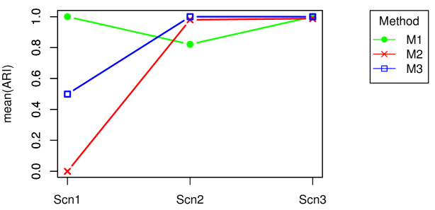
Figure 4: Performance of each method, given by the mean ARI of all replications from cases in each scenario: groups with similar trends and distinct peak locations (scenario 1); groups with distinct trends and similar peak locations (scenario 2); and groups with distinct trends and distinct peak locations (scenario 3). The clustering methods 1, 2 and 3 correspond to the three broken lines.

Figure 4 provides a rough summary of the simulation results by showing the ARI averaged over all cases of each scenario. The performance of a method is thus measured by three numbers. We note that no method is best in all scenarios. Method 2, which ignores the peak information, is never the best method. Method 1 is the best in scenario 1, and Method 3 is the best in scenarios 2 and 3. For a given dataset it is recommended to carry out a preliminary inspection to determine which scenario it corresponds to, before selecting the clustering method.

4 Application to real data

In this section we analyze two datasets, consisting of the lag distributions of all words of length $k=3$ and $k=5$ in the complete human genome. These datasets are denoted by $DD_{k}$ where $k$ identifies the word length. $DD_{3}$ consists of 64 distributions and $DD_{5}$ contains 1024 distributions. A preliminary visual inspection of these histograms revealed that there are substantial differences in both the trends and the peak structures, so in accordance with the conclusions of the simulation study we selected Method 3 (described in Section 2.6) for clustering the words in each dataset.

4.1 Data and data processing

We used the complete DNA sequence of the human genome assembly, downloaded from the website of the National Center for Biotechnology Information. The available assembled chromosomes (in version GRCh38.p2) were processed as separate sequences and all non-ACGT symbols were considered as sequence separators.

The counts of word lags were obtained by a dedicated C program able to handle large datasets (the haploid human genome has over 3 billion symbols). We analyzed the absolute frequences of the lags $j=k+1,\ldots,L$ where $L=1000$ for $k=3$ and $L=4000$ for $k=5$.

The R language was used to decompose the lag distributions, to perform the principal component analysis and the clustering and to carry out further statistical analysis. The R code used in this report, as well as the data sets and a script analyzing them and reproducing the figures can be downloaded from
https://wis.kuleuven.be/stat/robust/software .

4.2 Decomposing the lag distributions

In both datasets we first estimated the baseline distribution by LTS as described in Subsection 2.3, in which we set $L^{*}=200$ for $DD_{3}$ and $L^{*}=1500$ for $DD_{5}$. The peak functions were then estimated as described in Subsection 2.4.

4.3 Clustering words of length 3

Each distribution in $DD_{3}$ is summarized by 4 values, as the PCA retains 2 components for the peaks and 2 components for the baselines.

Figure 5 plots the validation indices against the number of clusters ($<10$). The CH index has a local maximum at 3 clusters and is high again at 6 clusters or more, whereas the silhouette index is highest for 2 clusters and the C index is lowest (best) for 2 clusters and gets low again for over 6 clusters. From the 3 indices together it would appear natural to select 2 clusters, for which $\mbox{CH}=108$, $S=0.68$ and $C=0.052$. The cluster $C_{1}$ has 8 elements, and cluster $C_{2}$ has 56.

Figure 5: Validation indices for clustering $DD_{3}$ by the number of clusters $nc$: the Calinsky-Harabasz index (left), silhouette coefficient (center) and C-index (right).

To test the stability of this clustering we follow the approach of Hennig [11]. We draw a so-called bootstrap sample, which is a random sample with replacement from the 64 objects in the $DD_{3}$ dataset. This creates a different dataset with 64 objects, some of which coincide. We then apply the same clustering method to it, set to 2 clusters. Let us call the new clusters $D_{a}$ and $D_{b}$. Then we compute the so-called Jaccard similarity coefficient of $C_{1}$ with the new clustering, defined as

$$J(C_{1})=\mbox{max}\Big{(}\frac{|C_{1}\cap D_{a}|}{|C_{1}\cup D_{a}|}\,,\frac{|C_{1}\cap D_{b}|}{|C_{1}\cup D_{b}|}\Big{)}\leqslant 1$$ (8)

where $|\ldots|$ stands for the number of elements. A high value $J(C_{1})$ indicates that $C_{1}$ is similar to one of the clusters of the new partition. We compute $J(C_{2})$ analogously. Then we repeat this whole procedure for a new bootstrap sample and so on, 200 times in all. The average of the 200 values of $J(C_{1})$ equals 0.952, which means that the cluster $C_{1}$ is very stable. For cluster $C_{2}$ we attain the stability index $0.978$ which is even higher.

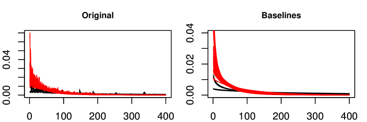
Figure 6: Clustering of the dataset $DD_{3}$ in clusters $C_{1}$ and $C_{2}$. The lag distributions are shown on the left, and the corresponding baselines on the right. Cluster $C_{1}$ is in black and $C2$ in red.

Figure 6 depicts the clusters $C_{1}$ and $C_{2}$. The lag distributions in $C_{1}$ are flatter than those in $C_{2}$. It turns out that all the words in $C_{1}$ contain the dinucleotide CG (known as CpG). In fact, $C_{1}$ consists exactly of the 8 words of length 3 that contain CG (i.e., ACG, CCG, GCG, TCG, CGA, CGC, CGG, CGT), so $C_{2}$ contains no words with CG. The special behaviour of the CG dinucleotide in the human genome is well reported in the literature. Although human DNA is generally depleted in the dinucleotide CpG (its occurrence is only 21% of what would be expected under randomness), the genome is punctuated by regions with a high frequency of CpG’s relative to the bulk genome. This DNA characteristic is related to the CpG methylation [6, 9]. We may conclude that the clustering of $DD_{3}$ has biological relevance.

It is worth noting that if one considers all k-means clusterings into 2 to 40 clusters, the second best silhouette coefficient is attained for 26 clusters, which also corresponds to the point where the CH index has a large increase and the C-index is very small ($CH=436$, $S=0.61$ and $C=0.0046$). In this partition with 26 clusters, over half of the clusters are formed by pairs of words that are reversed complements of each other, i.e., obtained by reversing the order of the word’s symbols and interchanging A-T and C-G. The similarity between lag patterns of reversed complements is a well-known feature described in the literature, see e.g. [26].

4.4 Clustering words of length 5

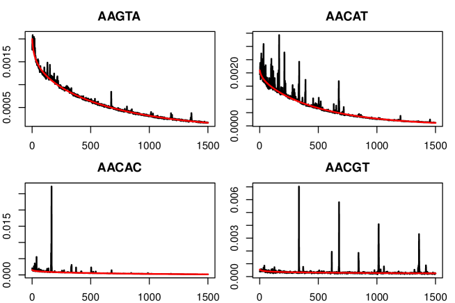
Figure 7: Lag distributions of some words of length $k=5$, with the corresponding baselines indicated in red.

Also the lag distributions of $DD_{5}$ contain quite distinct baselines and peak structures. Figure 7 shows four lag distributions, with their corresponding estimated baselines.

Our procedure retains 3 principal components for the peaks and 2 components for the baselines, so that each lag distribution is converted into 5 scores. Carrying out k-means clustering for different numbers of clusters yields the plots of validation indices in Figure 8. They do not all point to the same choice, however. The CH and S indices have local maxima at 2 and 6 clusters, while the C-index would support a choice of 5 or more clusters. It would appear that 2 or 6 clusters are appropriate.

Figure 8: Validation indices for clustering $DD_{5}$ by the number of clusters $nc$: the Calinsky-Harabasz index (left), average silhouette width (center) and C-index (right).

When choosing 2 clusters we obtain clusters with 278 and 746 members, and when choosing 6 clusters they have sizes 19, 92, 166, 141, 367 and 239.

We verified that both these partitions are very stable. For this we again drew 200 bootstrap samples, and partitioned each of them followed by computing the Jaccard similarity coefficient of the original clusters. In the case of 2 clusters the average Jaccard (stability) indices were 0.94 and 0.97. In the case of 6 clusters they were 0.84, 0.91, 0.93, 0.92, 0.93 and 0.93. Since we aim to decompose the $DD_{5}$ dataset of 1024 distributions into smaller groups with similar patterns, we will focus on the solution with 6 clusters from here onward.

The 6-cluster partition consists of two large clusters ($|C_{5}|=367$ and $|C_{6}|=239$), three middle-sized clusters ($|C_{2}|=92$, $|C_{3}|=166$ and $|C_{4}|=141$), and the much smaller cluster $C_{3}$ with only 19 elements. Figure 9 shows the lag distributions of each cluster. As a graphical summary we also consider the median function of each cluster, which in each domain point (lag) equals the median of the cluster’s function values in that point.

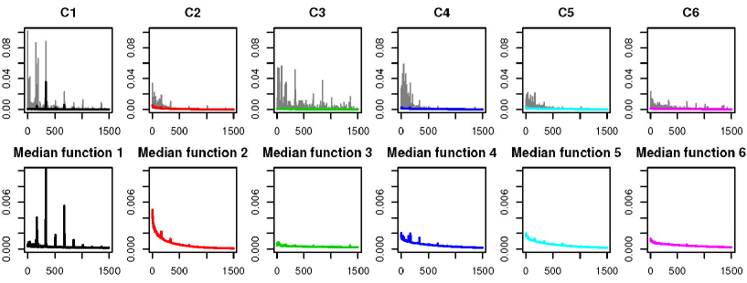
Figure 9: Clustering of $DD_{5}$ in six clusters. In each cluster the lag distributions are shown in grey, and the cluster’s median function is in color (top). The median functions are also shown with a scaled vertical axis (bottom).

We see the most pronounced peaks in the clusters $C_{1}$, $C_{3}$ and $C_{4}$. Those in the small cluster $C_{1}$ are the strongest. Several of them occur in the same location for most of the cluster members, which explains why they remain visible in the median function. The words in $C_{1}$ are listed in Table 4.

Table 4: List of words in cluster $C_{1}$ of the partition of $DD_{5}$ in six clusters.

AAACG	AACGG	ACGGG	AGCGC	CGAGA	CGCTT
CGGGA	CGTTC	CGTTG	CTTCG	GAGGC	GCCTC
GCGCT	GCGTT	TCGTA	TCGTT	TCTCG	TTCGT
TTTCG

The distributions in $C_{4}$ have most of their peaks before lag 500, with little going on after that. Cluster $C_{3}$ is quite different, as strong peaks occur over the whole domain. The distributions in clusters $C_{2}$, $C_{5}$ and $C_{6}$ have rather small peaks, so few major irregularities. Their main difference is in the baselines: those of $C_{2}$ have a high rate $\lambda$, whereas the baselines of $C_{6}$ are much flatter.

We also explore the composition of the words in each cluster, by computing the percentage of words that contain a given dinucleotide or trinucleotide. Clusters $C_{1}$, $C_{2}$ and $C_{3}$ stand out in this respect. Cluster $C_{2}$ contains the largest proportion of words with the dinucleotides AA (47%) and TT (49%), which is also reflected in the high frequency of AAA and TTT (25% and 26%, respectively). The clusters $C_{1}$ and $C_{3}$ have a lot of words containing the dinucleotide CG (89% and 98%). This is very different from the other clusters: only 9% of the words in $C_{2}$ contain CG, in $C_{4}$ this is 11%, in $C_{5}$ only 1%, and in $C_{6}$ 16%. Even though both $C_{1}$ and $C_{3}$ have many CG dinucleotides, these occur in different trinucleotides: $C_{1}$ has many words containing CGT and TCG (both 32%), whereas in $C_{3}$ many words contain CGA (27%) and ACG (23%).

5 Summary and conclusions

In this work we have proposed a methodology for decomposing the lag distribution of a genomic word into the sum of a baseline distribution (the ‘trend’) and a peak function. The baseline component is estimated by robustly fitting a parametric function to the data distribution, in which the residuals are made homoskedastic and the robustness to outliers is essential. The peak function is then obtained by comparing the absolute frequency at each lag to a quantile of a Poisson distribution.

When analyzing a dataset consisting of many genomic words we can apply principal component analysis to the set of baselines and the set of peak functions, which greatly reduces the dimensionality. This lower-dimensional data set has uncorrelated scores and retains much of the original information, such as that in the Euclidean distances. This allows us to carry out k-means clustering, in which we have the choice whether to use only the baseline information, only the peak information, or both. The performance of this approach was evaluated by a simulation study, which concluded that in situations where both distinct baselines as well as distinct peak functions occur, the clustering procedure using the combined information performs very well.

This procedure was applied to the data set $DD_{3}$ of all genomic words of 3 symbols in human DNA, as well as the set $DD_{5}$ of all words of length 5. This resulted in clusters of words with specific distribution patterns. By looking at the composition of the words in each cluster we found connections with the frequency of certain trinucleotides and dinucleotides, such as CG which plays a particular biological role.

Topics for further research are the analysis of longer words, and the application of other statistical methods (such as classification) on genomic data after applying the decomposition technique developed here.

Acknowledgements

This work was partially supported by the Portuguese Foundation for Science and Technology (FCT), Center for Research & Development in Mathematics and Applications (CIDMA) and Institute of Biomedicine (iBiMED), within projects UID/MAT/04106/2013 and UID/BIM/04501/ 2013. A. Tavares acknowledges the PhD grant PD/BD/105729/ 2014 from the FCT. The research of P. Brito was financed by the ERDF - European Regional Development Fund through the Operational Programme for Competitiveness and Internationalization - COMPETE 2020 Programme within project POCI-01-0145-FEDER-006961, and by the FCT as part of project UID/EEA/50014/2013. The research of J. Raymaekers and P. J. Rousseeuw was supported by projects of Internal Funds KU Leuven.

References

- [1] Abramowitz, M., Stegun, I.A.: Handbook of mathematical functions: with formulas, graphs, and mathematical tables, vol. 55. Courier Corporation (1964)
- [2] Afreixo, V., Rodrigues, J.M., Bastos, C.A.: Analysis of single-strand exceptional word symmetry in the human genome: new measures. Biostatistics 16(2), 209–221 (2014)
- [3] Bajic, V.B., Seah, S.H.: Dragon gene start finder: an advanced system for finding approximate locations of the start of gene transcriptional units. Genome Research 13(8), 1923–1929 (2003)
- [4] Burge, C., Campbell, A.M., Karlin, S.: Over-and under-representation of short oligonucleotides in DNA sequences. Proceedings of the National Academy of Sciences 89(4), 1358–1362 (1992)
- [5] Caliński, T., Harabasz, J.: A dendrite method for cluster analysis. Communications in Statistics 3(1), 1–27 (1974)
- [6] Consortium, I.H.G.S., et al.: Initial sequencing and analysis of the human genome. Nature 409(6822), 860 (2001)
- [7] Deaton, A.M., Bird, A.: CpG islands and the regulation of transcription. Genes & development 25(10), 1010–1022 (2011)
- [8] Fu, J.C.: Distribution theory of runs and patterns associated with a sequence of multi-state trials. Statistica Sinica pp. 957–974 (1996)
- [9] Gardiner-Garden, M., Frommer, M.: CpG islands in vertebrate genomes. Journal of molecular biology 196(2), 261–282 (1987)
- [10] Guerra, L., Robles, V., Bielza, C., Larrañaga, P.: A comparison of clustering quality indices using outliers and noise. Intelligent Data Analysis 16(4), 703–715 (2012)
- [11] Hennig, C.: Dissolution point and isolation robustness: Robustness criteria for general cluster analysis methods. Journal of Multivariate Analysis 99(6), 1154–1176 (2008)
- [12] Hubert, L., Arabie, P.: Comparing partitions. Journal of Classification 2(1), 193–218 (1985)
- [13] Hubert, L.J., Levin, J.R.: A general statistical framework for assessing categorical clustering in free recall. Psychological Bulletin 83(6), 1072 (1976)
- [14] Jacinto, F.V., Esteller, M.: Mutator pathways unleashed by epigenetic silencing in human cancer. Mutagenesis 22(4), 247–253 (2007)
- [15] Kaufman, L., Rousseeuw, P.J.: Finding Groups in Data. Wiley-Interscience, NY (1990)
- [16] Leung, M.Y., Marsh, G.M., Speed, T.P.: Over-and underrepresentation of short DNA words in herpesvirus genomes. Journal of Computational Biology 3(3), 345–360 (1996)
- [17] Liu, Y., Li, Z., Xiong, H., Gao, X., Wu, J.: Understanding of internal clustering validation measures. In: 10th IEEE International Conference on Data Mining (ICDM), pp. 911–916. IEEE (2010)
- [18] MacIsaac, K.D., Fraenkel, E.: Practical strategies for discovering regulatory DNA sequence motifs. PLoS Computational Biology 2(4), e36 (2006)
- [19] Milligan, G.W., Cooper, M.C.: An examination of procedures for determining the number of clusters in a data set. Psychometrika 50(2), 159–179 (1985)
- [20] Milligan, G.W., Cooper, M.C.: A study of the comparability of external criteria for hierarchical cluster analysis. Multivariate Behavioral Research 21(4), 441–458 (1986). DOI 10.1207/s15327906mbr2104_5. PMID: 26828221
- [21] Nakamoto, T.: Evolution and the universality of the mechanism of initiation of protein synthesis. Gene 432(1), 1–6 (2009)
- [22] Percus, J.K.: Mathematics of genome analysis, vol. 17. Cambridge University Press (2002)
- [23] Rousseeuw, P.J.: Least median of squares regression. Journal of the American Statistical Association 79, 871–880 (1984)
- [24] Rousseeuw, P.J.: Silhouettes: a graphical aid to the interpretation and validation of cluster analysis. Journal of Computational and Applied Mathematics 20, 53–65 (1987)
- [25] Saxonov, S., Berg, P., Brutlag, D.L.: A genome-wide analysis of CpG dinucleotides in the human genome distinguishes two distinct classes of promoters. Proceedings of the National Academy of Sciences 103(5), 1412–1417 (2006)
- [26] Tavares, A.H., Afreixo, V., Rodrigues, J.a.M., Bastos, C.A.C.: The symmetry of oligonucleotide distance distributions in the human genome. In: ICPRAM (2), pp. 256–263 (2015)
- [27] Tavares, A.H.M.P., Afreixo, V., Rodrigues, J.a.M., Bastos, C.A.C., Pinho, A.J., Ferreira, P.J.S.G., Brito, P.: Detection of exceptional genomic words: A comparison between species. In: Proceedings of 22nd International Conference on Computational Statistics (COMPSTAT), pp. 255–264 (2016)
- [28] Tavares, A.H.M.P., Pinho, A.J., Silva, R.M., Rodrigues, J.M.O.S., Bastos, C.A.C., Ferreira, P.J.S.G., Afreixo, V.: DNA word analysis based on the distribution of the distances between symmetric words. Scientific reports 7(1), 728 (2017)