Abstract

We study nonlinear cosmological perturbations and their possible non-Gaussian character in an extended non-minimal inflation where gravity is coupled non-minimally to both the scalar field and its derivatives. By expansion of the action up to the third order, we focus on the non-linearity and non-Gaussianity of perturbations in comparison with recent observational data. By adopting an inflation potential of the form $V(\phi)=\frac{1}{n}\lambda\phi^{n}$, we show that for $n=4$, for instance, this extended model is consistent with observation if $0.013<\lambda<0.095$ in appropriate units. By restricting the equilateral amplitude of non-Gaussianity to the observationally viable values, the coupling parameter $\lambda$ is constraint to the values $\lambda<0.1$.
PACS: 98.80.Bp, 98.80.Cq , 98.80.Es
Key Words: Cosmological Inflation, Structure Formation, Perturbations, Non-Minimal Inflationary Models, Observational Data

1 Introduction

The idea of cosmological inflation is capable to address some problems of the standard big bang theory, such as the horizon, flatness and monopole problems. Also, it can provide a reliable mechanism for generation of density perturbations responsible for structure formation and therefore temperature anisotropies in Cosmic Microwave Background (CMB)spectrum [1-8]. There are a wide variety of cosmological inflation models where viability of their predictions in comparison with observations makes them to be acceptable or unacceptable (see for instance [9] for this purpose). The simplest inflationary model is a single scalar field scenario in which inflation is driven by a scalar field called the inflaton that predicts adiabatic, Gaussian and scale-invariant fluctuations [10]. But, recently observational data have revealed some degrees of scale-dependence in the primordial density perturbations. Also, Planck team have obtained some constraints on the primordial non-Gaussianity [11-13]. Therefore, it seems that extended models of inflation which can explain or address this scale-dependence and non-Gaussianity of perturbations are more desirable. There are a lot of studies in this respect, some of which can be seen in Refs. [14-19] with references therein. Among various inflationary models, the non-minimal models have attracted much attention. Non-minimal coupling of the inflaton field and gravitational sector is inevitable from the renormalizability of the corresponding field theory (see for instance [20]). Cosmological inflation driven by a scalar field non-minimally coupled to gravity are studied, for instance, in Refs. [21-28]. There were some issues on the unitarity violation with non-minimal coupling (see for instance, Refs. [29-31]) which have forced researchers to consider possible coupling of the derivatives of the scalar field with geometry [32]. In fact, it has been shown that a model with nonminimal coupling between the kinetic terms of the inflaton (derivatives of the scalar field) and the Einstein tensor preserves the unitary bound during inflation [33]. Also, the presence of nonminimal derivative coupling is a powerful tool to increase the friction of an inflaton rolling down its own potential [33]. Some authors have considered the model with this coupling term and have studied the early time accelerating expansion of the universe as well as the late time dynamics [34-36]. In this paper we extend the non-minimal inflation models to the case that a canonical inflaton field is coupled non-minimally to the gravitational sector and in the same time the derivatives of the field are also coupled to the background geometry (Einstein’s tensor). This model provides a more realistic framework for treating cosmological inflation in essence. We study in details the cosmological perturbations and possible non-Gaussianities in the distribution of these perturbations in this non-minimal inflation. We expand the action of the model up to the third order and compare our results with observational data from Planck2015 to see the viability of this extended model. In this manner we are able to constraint parameter space of the model in comparison with observation.

2 Field Equations

We consider an inflationary model where both a canonical scalar field and its derivatives are coupled non-minimally to gravity. The four-dimensional action for this model is given by the following expression:

$$S=\frac{1}{2}\int d^{4}x\sqrt{-g}\Bigg{[}M_{p}^{2}f(\phi)R+\frac{1}{\widetilde{M}^{2}}G_{\mu\nu}\partial^{\mu}\phi\partial^{\nu}\phi-2V(\phi)\Bigg{]}\,,$$ (1)

where $M_{p}$ is a reduced planck mass, $\phi$ is a canonical scalar field, $f(\phi)$ is a general function of the scalar field and $\widetilde{M}$ is a mass parameter. The energy-momentum tensor is obtained from action (1) as follows

$T_{\mu\nu}=\frac{1}{2\widetilde{M}^{2}}\bigg{[}\nabla_{\mu}\nabla_{\nu}(\nabla^{\alpha}\phi\nabla_{\alpha}\phi)-g_{\mu\nu}\Box(\nabla^{\alpha}\phi\nabla_{\alpha}\phi)+g_{\mu\nu}g^{\alpha\rho}g^{\beta\lambda}\nabla_{\rho}\nabla_{\lambda}(\nabla_{\alpha}\phi\nabla_{\beta}\phi)$

$$+\Box(\nabla_{\mu}\phi\nabla_{\nu}\phi)\bigg{]}-\frac{g^{\alpha\beta}}{\widetilde{M}^{2}}\nabla_{\beta}\nabla_{\mu}(\nabla_{\alpha}\phi\nabla_{\nu}\phi)-M_{p}^{2}\nabla_{\mu}\nabla_{\nu}f(\phi)+M_{p}^{2}g_{\mu\nu}\Box f(\phi)+g_{\mu\nu}V(\phi)\,.$$ (2)

On the other hand, variation of the action (1) with respect to the scalar field gives the scalar field equation of motion as

$$\frac{1}{2}M_{p}^{2}Rf^{\prime}(\phi)-\frac{1}{\widetilde{M}^{2}}G^{\mu\nu}\nabla_{\mu}\nabla_{\nu}\phi-V^{\prime}(\phi)=0\,,$$ (3)

where a prime denotes derivative with respect to the scalar field. We consider a spatially flat Friedmann-Robertson-Walker (FRW) line element as

$$ds^{2}=-dt^{2}+a^{2}(t)\delta_{ij}dx^{i}dx^{j}\,,$$ (4)

where $a(t)$ is scale factor. Now, let’s assume that $f(\phi)=\frac{1}{2}\phi^{2}$. In this framework, $T_{\mu\nu}$ leads to the following energy density and pressure for this model respectively

$$\rho=\frac{9H^{2}}{2\widetilde{M}^{2}}\dot{\phi}^{2}-\frac{3}{2}M_{p}^{2}H\phi(2\dot{\phi}+H\phi)+V(\phi)$$ (5)

$$p=-\frac{3}{2}\frac{H^{2}\dot{\phi}^{2}}{\widetilde{M}^{2}}-\frac{\dot{\phi}^{2}\dot{H}}{\widetilde{M}^{2}}-\frac{2H}{\widetilde{M}^{2}}\dot{\phi}\ddot{\phi}$$

$$+\frac{1}{2}M_{p}^{2}\Bigg{[}2\dot{H}\phi^{2}+3H^{2}\phi^{2}+4H\phi\dot{\phi}+2\phi\ddot{\phi}+2\dot{\phi}\Bigg{]}-V(\phi)\,,$$ (6)

where a dot refers to derivative with respect to the cosmic time. The equations of motion following from action (1) are

$$H^{2}=\frac{1}{3M_{p}^{2}}\Bigg{[}-\frac{3}{2}M_{p}^{2}H\phi(2\dot{\phi}+H\phi)+\frac{9H^{2}}{2\widetilde{M}^{2}}\dot{\phi}^{2}+V(\phi)\Bigg{]}\,,$$ (7)

$$\dot{H}=-\frac{1}{2M_{p}^{2}}\Bigg{[}\dot{\phi}^{2}\bigg{(}\frac{3H^{2}}{\widetilde{M}^{2}}-\frac{\dot{H}}{\widetilde{M}^{2}}\bigg{)}-\frac{2H}{\widetilde{M}^{2}}\dot{\phi}\ddot{\phi}-\frac{3}{2}M_{p}^{2}H\phi(2\dot{\phi}+H\phi)$$

$$+\frac{1}{2}M_{p}^{2}\bigg{(}(2\dot{H}+3H^{2})\phi^{2}+4H\phi\dot{\phi}+2\phi\ddot{\phi}+2\dot{\phi}^{2}\bigg{)}\Bigg{]}$$ (8)

$$-3M_{p}^{2}(2H^{2}+\dot{H})\phi+\frac{3H^{2}}{\widetilde{M}^{2}}\ddot{\phi}+3H\bigg{(}\frac{3H^{2}}{\widetilde{M}^{2}}+\frac{2\dot{H}}{\widetilde{M}^{2}}\bigg{)}\dot{\phi}+V^{\prime}(\phi)=0\,.$$ (9)

The slow-roll parameters in this model are defined as

$$\epsilon\equiv-\frac{\dot{H}}{H^{2}}\,\,\,\,,\,\,\,\,\eta\equiv-\frac{1}{H}\frac{\ddot{H}}{\dot{H}}\,.$$ (10)

To have inflationary phase, $\epsilon$ and $\eta$ should satisfy slow-roll conditions($\epsilon\ll 1$ , $\eta\ll 1$). In our setup, we find the following result

$$\epsilon=\bigg{[}1+\frac{\phi^{2}}{2}-\frac{\dot{\phi^{2}}}{2\widetilde{M}^{2}M_{p}^{2}}\bigg{]}^{-1}\bigg{[}\frac{3\dot{\phi}^{2}}{2\widetilde{M}^{2}M_{p}^{2}}+\frac{\phi\dot{\phi}}{2H}+\frac{\ddot{\phi}}{H\dot{\phi}}\bigg{(}\frac{\phi\dot{\phi}}{2H}-\frac{\dot{\phi^{2}}}{\widetilde{M}^{2}M_{p}^{2}}\bigg{)}\bigg{]}$$ (11)

and

$$\eta=-2\epsilon-\frac{\dot{\epsilon}}{H\epsilon}\,.$$ (12)

Within the slow-roll approximation, equations (7),(8) and (9) can be written respectively as

$$H^{2}\simeq\frac{1}{3M_{p}^{2}}\Bigg{[}-\frac{3}{2}M_{p}^{2}H^{2}\phi^{2}+V(\phi)\Bigg{]}\,,$$ (13)

$$\dot{H}\simeq-\frac{1}{2M_{p}^{2}}\Bigg{[}\frac{3H^{2}\dot{\phi}^{2}}{\widetilde{M}^{2}}-M_{p}^{2}H\phi\dot{\phi}+M_{p}^{2}\dot{H}\phi^{2}\Bigg{]}\,,$$ (14)

and

$$-6M_{p}^{2}H^{2}\phi+\frac{9H^{3}\dot{\phi}}{\widetilde{M}^{2}}+V^{\prime}(\phi)\simeq 0\,.$$ (15)

The number of e-folds during inflation is defined as

$${\cal N}=\int_{t_{hc}}^{t_{e}}H\,dt\,,$$ (16)

where $t_{hc}$ and $t_{e}$ are time of horizon crossing and end of inflation respectively. The number of e-folds in the slow-roll approximation in our setup can be expressed as follows

$${\cal N}\simeq\int_{\phi_{hc}}^{\phi_{e}}\frac{V(\phi)d\phi}{M_{p}^{2}\bigg{(}1+\frac{1}{2}\phi^{2}\bigg{)}\Bigg{[}2M_{p}^{2}\widetilde{M}^{2}\phi-M_{p}^{2}\widetilde{M}^{2}\frac{V^{\prime}(\phi)}{V(\phi)}\bigg{(}1+\frac{1}{2}\phi^{2}\bigg{)}\Bigg{]}}\,.$$ (17)

After providing the basic setup of the model, for testing cosmological viability of this extended model we treat the perturbations in comparison with observation.

3 Second-Order Action: Linear Perturbations

In this section, we study linear perturbations around the homogeneous background solution. To this end, the first step is expanding the action (1) up to the second order in small fluctuations. It is convenient to work in the ADM formalism given by [37]

$$ds^{2}=-N^{2}dt^{2}+h_{ij}(N^{i}dt+dx^{i})(N^{j}dt+dx^{j})\,,$$ (18)

where $N^{i}$ is the shift vector and $N$ is the lapse function. We expand the lapse function and shift vector to $N=1+2\Phi$ and $N^{i}=\delta^{ij}\partial_{j}\Upsilon$ respectively, where $\Phi$ and $\Upsilon$ are three-scalars. Also, $h_{ij}=a^{2}(t)[(1+2\Psi)\delta_{ij}+\gamma_{ij}]$, where $\Psi$ is spatial curvature perturbation and $\gamma_{ij}$ is shear three-tensor which is traceless and symmetric. In the rest of our study, we choose $\delta\Phi=0$ and $\gamma_{ij}=0$. By taking into account the scalar perturbations in linear-order, the metric (18) is written as (see for instance [38])

$$ds^{2}=-(1+2\Phi)dt^{2}+2\partial_{i}\Upsilon dtdx^{i}+a^{2}(t)(1+2\Psi)\delta_{ij}dx^{i}dx^{j}\,.$$ (19)

Now by replacing metric (19) in action (1) and expanding the action up to the second-order in perturbations, we find (see for instance [39,40])

$$S^{(2)}=\int dtdx^{3}a^{3}\Bigg{[}-\frac{3}{2}(M_{p}^{2}\phi^{2}-\frac{\dot{\phi}^{2}}{\widetilde{M}^{2}})\dot{\Psi}^{2}+\frac{1}{a^{2}}((M_{p}^{2}\phi^{2}-\frac{\dot{\phi}^{2}}{\widetilde{M}^{2}})\dot{\Psi}$$

$$-(M_{p}^{2}H\phi^{2}+M_{p}^{2}\phi\dot{\phi}-\frac{3H\dot{\phi}^{2}}{\widetilde{M}^{2}})\Phi)\partial^{2}\Upsilon-\frac{1}{a^{2}}(M_{p}^{2}\phi^{2}-\frac{\dot{\phi}^{2}}{\widetilde{M}^{2}})\Phi\partial^{2}\Psi$$

$$+3(M_{p}^{2}H\phi^{2}+M_{p}^{2}\phi\dot{\phi}-\frac{3H\dot{\phi}^{2}}{\widetilde{M}^{2}})\Phi\dot{\Psi}+3H(-\frac{1}{2}M_{p}^{2}H\phi^{2}-M_{p}^{2}\phi\dot{\phi}$$

$$+\frac{3H\dot{\phi}^{2}}{\widetilde{M}^{2}})\Phi^{2}+\frac{1}{2a^{2}}(M_{p}^{2}\phi^{2}+\frac{\dot{\phi}^{2}}{\widetilde{M}^{2}})(\partial\Psi)^{2}\Bigg{]}\,.$$ (20)

By variation of action (20) with respect to $N$ and $N^{i}$ we find

$$\Phi=\frac{M_{p}^{2}\phi^{2}-\frac{\dot{\phi}^{2}}{\widetilde{M}^{2}}}{M_{p}^{2}H\phi^{2}+M_{p}^{2}\phi\dot{\phi}-\frac{3H\dot{\phi}^{2}}{\widetilde{M}^{2}}}\dot{\Psi}\,,$$ (21)

$$\partial^{2}\Upsilon=\frac{2a^{2}}{3}\frac{(-\frac{9}{2}M_{p}^{2}H^{2}\phi^{2}-9M_{p}^{2}H\phi\dot{\phi}+\frac{27H^{2}\dot{\phi}^{2}}{\widetilde{M}^{2}})}{(M_{p}^{2}H\phi^{2}+M_{p}^{2}\phi\dot{\phi}-\frac{3H\dot{\phi}^{2}}{\widetilde{M}^{2}})}$$

$$+3\dot{\Psi}a^{2}-\frac{M_{p}^{2}\phi^{2}-\frac{\dot{\phi}^{2}}{\widetilde{M}^{2}}}{M_{p}^{2}H\phi^{2}+M_{p}^{2}\phi\dot{\phi}-\frac{3H\dot{\phi}^{2}}{\widetilde{M}^{2}}}\dot{\Psi}\,.$$ (22)

Finally the second order action can be rewritten as follows

$$S^{(2)}=\int dtdx^{3}a^{3}\vartheta_{s}\bigg{[}\dot{\Psi}^{2}-\frac{c_{s}^{2}}{a^{2}}(\partial\Psi)^{2}\bigg{]}$$ (23)

where by definition

$$\vartheta_{s}\equiv 6\frac{(M_{p}^{2}\phi^{2}-\frac{\dot{\phi}^{2}}{\widetilde{M}^{2}})^{2}(-\frac{1}{2}M_{p}^{2}H^{2}\phi^{2}-M_{p}^{2}H\phi\dot{\phi}+\frac{3}{\widetilde{M}^{2}}H^{2}\dot{\phi}^{2})}{(M_{p}^{2}H\phi^{2}+M_{p}^{2}\phi\dot{\phi}-\frac{3}{\widetilde{M}^{2}}H\dot{\phi}^{2})^{2}}+3(\frac{1}{2}M_{p}^{2}\phi^{2}-\frac{1}{2\widetilde{2}}\dot{\phi}^{2})$$ (24)

and

$$c_{s}^{2}\equiv\frac{3}{2}\bigg{\{}(M_{p}^{2}\phi^{2}-\frac{\dot{\phi}^{2}}{\widetilde{M}^{2}})^{2}(M_{p}^{2}H\phi^{2}+M_{p}^{2}\phi\dot{\phi}-\frac{3H\dot{\phi}^{2}}{\widetilde{M}^{2}})H$$

$$-(M_{p}^{2}H\phi^{2}+M_{p}^{2}\phi\dot{\phi}-\frac{3H\dot{\phi}^{2}}{\widetilde{M}^{2}})^{2}(M_{p}^{2}\phi^{2}-\frac{\dot{\phi}^{2}}{\widetilde{M}^{2}})$$

$$4(M_{p}^{2}\phi^{2}-\frac{\dot{\phi}^{2}}{\widetilde{M}^{2}})(M_{p}^{2}\phi\dot{\phi}-\frac{\dot{\phi}\ddot{\phi}}{\widetilde{M}^{2}})(M_{p}^{2}H\phi^{2}+M_{p}^{2}\phi\dot{\phi}-\frac{3H\dot{\phi}^{2}}{\widetilde{M}^{2}})$$

$$-(M_{p}^{2}-\frac{\dot{\phi}^{2}}{\widetilde{M}^{2}})^{2}(M_{p}^{2}\dot{H}\phi^{2}+2M_{p}^{2}H\phi\dot{\phi}M_{p}^{2}\dot{\phi}^{2}+M_{p}^{2}\phi\ddot{\phi}-\frac{3\dot{H}\dot{\phi}^{2}}{\widetilde{M}^{2}}-\frac{6}{\widetilde{M}^{2}}H\dot{\phi}\ddot{\phi})\bigg{\}}$$

$$\bigg{\{}9[\frac{1}{2}M_{p}^{2}\phi^{2}-\frac{\dot{\phi}^{2}}{2\widetilde{M}^{2}}][4(\frac{1}{2}M_{p}^{2}\phi^{2}-\frac{\dot{\phi}^{2}}{2\widetilde{M}^{2}})(-\frac{1}{2}M_{p}^{2}H^{2}\phi^{2}-M_{p}^{2}H\phi\dot{\phi}+\frac{3}{M\widetilde{{}^{2}}H^{2}\dot{\phi}^{2}})$$

$$+(M_{p}^{2}H\phi^{2}+M_{p}^{2}\phi\dot{\phi}-\frac{3H\dot{\phi}^{2}}{\widetilde{M}^{2}})^{2}]\bigg{\}}^{-1}\,.$$ (25)

In order to obtain quantum perturbations $\Psi$, we can find equation of motion of the curvature perturbation by varying action (23) which follows

$$\ddot{\Psi}+\bigg{(}3H+\frac{\dot{\vartheta_{s}}}{\vartheta_{s}}\bigg{)}+\frac{c_{s}^{2}k^{2}}{a^{2}}\Psi=0\,.$$ (26)

By solving the above equation up to the lowest order in slow-roll approximation, we find

$$\Psi=\frac{iH\exp(-ic_{s}k\tau)}{2c_{s}^{\frac{3}{2}}\sqrt{k^{3}}\vartheta_{s}}(1+ic_{s}k\tau)\,.$$ (27)

By using the two-point correlation functions we can study power spectrum of curvature perturbation in this setup. We find two-point correlation function by obtaining vacuum expectation value at the end of inflation. We define the power spectrum $P_{s}$, as

$$\langle 0|\Psi(0,\textbf{k}_{1})\Psi(0,\textbf{k}_{2})|0\rangle=\frac{2\pi^{2}}{k^{3}}P_{s}(2\pi)^{3}\delta^{3}(\textbf{k}_{1}+\textbf{k}_{2})\,,$$ (28)

where

$$P_{s}=\frac{H^{2}}{8\pi^{2}\vartheta_{s}c_{s}^{3}}\,.$$ (29)

The spectral index of scalar perturbations is given by (see Refs. [41-43] for more details on the cosmological perturbations in generalized gravity theories and also inflationary spectral index in these theories.)

$$n_{s}-1=\frac{d\ln P_{s}}{d\ln k}|_{c_{s}k=aH}=-2\epsilon-\delta_{F}-\eta_{s}-S$$ (30)

where by definition

$$\delta_{F}=\frac{\dot{f}}{H(1+f)}\,\,\,\,,\,\,\,\,\eta_{s}=\frac{\dot{\epsilon_{s}}}{H\epsilon_{s}}\,\,\,\,,\,\,\,\,S=\frac{\dot{c_{s}}}{Hc_{s}}$$ (31)

also

$$\epsilon_{s}=\frac{\vartheta_{s}c_{s}^{2}}{M_{pl}^{2}(1+f)}.$$ (32)

we obtain finally

$$n_{s}-1=-2\epsilon-\frac{1}{H}\frac{d\ln c_{s}}{dt}-\frac{1}{H}\frac{d\ln[2H(1+\frac{\phi^{2}}{2})\epsilon+\phi\dot{\phi}]}{dt}\,,$$ (33)

which shows the scale dependence of perturbations due to deviation of $n_{s}$ from $1$.

Now we study tensor perturbations in this setup. To this end, we write the metric as follows

$$ds^{2}=-dt^{2}+a(t)^{2}(\delta_{ij}+T_{ij})dx^{i}dx^{j}\,,$$ (34)

where $T_{ij}$ is a spatial shear 3-tensor which is transverse and traceless. It is convenient to write $T_{ij}$ in terms of two polarization modes, as follows

$$T_{ij}=T_{+}e^{+}_{ij}+T^{\times}e^{\times}_{ij}\,,$$ (35)

where $e^{+}_{ij}$ and $e^{\times}_{ij}$ are the polarization tensors. In this case the second order action for the tensor mode can de written as

$$S_{T}=\int dtdx^{3}a^{3}\vartheta_{T}\bigg{[}\dot{T}_{(+,\times)}^{2}-\frac{c_{T}^{2}}{a^{2}}(\partial T_{(+,\times)})^{2}\bigg{]}\,,$$ (36)

where by definition

$$\vartheta_{T}\equiv\frac{1}{8}(M_{p}^{2}\phi^{2}-\frac{\dot{\phi}^{2}}{\widetilde{M}^{2}})$$ (37)

and

$$c_{T}^{2}\equiv\frac{\widetilde{M}^{2}M_{p}^{2}\phi^{2}+\dot{\phi}^{2}}{\widetilde{M}^{2}M_{p}^{2}\phi^{2}-\dot{\phi}^{2}}\,.$$ (38)

Now, the amplitude of tensor perturbations is given by

$$P_{T}=\frac{H^{2}}{2\pi^{2}\vartheta_{T}c_{T}^{3}}\,,$$ (39)

where we have defined the tensor spectral index as

$$n_{T}\equiv\frac{d\ln P_{T}}{d\ln k}|_{c_{T}k=aH}\,=-2\epsilon-\delta_{F}.$$ (40)

By using above equations we get finally

$$n_{T}=-2\epsilon-\frac{\phi\dot{\phi}}{H(1+\frac{\phi^{2}}{2})}\,.$$ (41)

The tensor-to-scalar ratio as an important observational quantity in our setup is given by

$$r=\frac{P_{T}}{P_{s}}=16c_{s}\bigg{(}\epsilon+\frac{\phi\dot{\phi}}{2H(1+\frac{\phi^{2}}{2})}+O(\epsilon^{2})\bigg{)}\simeq-8c_{s}n_{T}$$ (42)

which yields the standard consistency relation.

4 Third-Order Action: Non-Gaussianity

Since a two-point correlation function of the scalar perturbations gives no information about possible non-Gaussian feature of distribution, we study higher-order correlation functions. A three-point correlation function is capable to give the required information. For this purpose, we should expand action (1) up to the third order in small fluctuations around the homogeneous background solutions. In this respect we obtain

$S^{(3)}=\int dtdx^{3}a^{3}\bigg{\{}3\Phi^{3}[M_{p}^{2}H^{2}(1+\frac{\phi^{2}}{2})+M_{p}^{2}H\phi\dot{\phi}-\frac{5}{\widetilde{M^{2}}}H^{2}\dot{\phi^{2}}]+\Phi^{2}[9\Psi(-\frac{1}{2}M_{p}^{2}\phi^{2}-M_{p}^{2}H\phi\dot{\phi}$ $+\frac{3}{\widetilde{M}}H^{2}\dot{\phi}^{2})+6\dot{\Psi}(-M_{p}^{2}H(1+\frac{\phi^{2}}{2})-\frac{1}{2}M_{p}^{2}\phi\dot{\phi}\frac{3}{\widetilde{M}^{2}}H\dot{\phi}^{2})-\frac{\dot{\phi}^{2}}{\widetilde{M}^{2}a^{2}}\partial^{2}\Psi-\frac{2}{a^{2}}\partial^{2}\Upsilon(-M_{p}^{2}H$ $(1+\frac{\phi^{2}}{2})-\frac{1}{2}M_{p}^{2}\phi\dot{\phi}\frac{3}{\widetilde{M}^{2}}H\dot{\phi}^{2})]+\Phi[\frac{1}{a^{2}}(-M_{p}^{2}H\phi^{2}-M_{p}^{2}\phi\dot{\phi}+\frac{3H\dot{\phi}^{2}}{\widetilde{M}^{2}})\partial_{i}\Psi\partial_{i}\Upsilon-9(-M_{p}^{2}H\phi^{2}-M_{p}^{2}\phi\dot{\phi}+$ $\frac{3H\dot{\phi}^{2}}{\widetilde{M}^{2}})\dot{\Psi}\Psi+\frac{1}{2a^{4}}(M_{p}^{2}(1+\frac{\phi^{2}}{2})+\frac{3}{2}\frac{\dot{\phi}^{2}}{\widetilde{M}^{2}})(\partial_{i}\partial_{j}\Upsilon\partial_{i}\partial_{j}\Upsilon-\partial^{2}\Upsilon\partial^{2}\Upsilon)+\frac{1}{a^{2}}(-M_{p}^{2}H\phi^{2}-M_{p}^{2}\phi\dot{\phi}+\frac{3H\dot{\phi}^{2}}{\widetilde{M}^{2}})\Psi\partial^{2}\Upsilon$ $+\frac{4}{2a^{2}}(M_{p}^{2}(1+\frac{\phi^{2}}{2})+\frac{3}{2}\frac{\dot{\phi}^{2}}{\widetilde{M}^{2}})\dot{\Psi}\partial^{2}\Upsilon+\frac{1}{a^{2}}(-M_{p}^{2}\phi^{2}+\frac{\dot{\phi}}{\widetilde{M}^{2}})\Psi\partial^{2}\Psi+\frac{1}{2a^{2}}(-M_{p}^{2}\phi^{2}+\frac{\dot{\phi}}{\widetilde{M}^{2}})(\partial\Psi)^{2}-6(M_{p}^{2}(1+\frac{\phi^{2}}{2})+$ $\frac{3}{2}\frac{\dot{\phi}^{2}}{\widetilde{M}^{2}})\dot{\Psi}^{2}]+\frac{1}{2a^{2}}(M_{p}^{2}\phi^{2}+\frac{\dot{\phi}^{2}}{\widetilde{M}^{2}})\Psi(\partial\Psi)^{2}+\frac{9}{2}(-M_{p}^{2}\phi^{2}+\frac{\dot{\phi}}{\widetilde{M}^{2}})\dot{\Psi^{2}}\Psi-\frac{1}{a^{2}}(-M_{p}^{2}\phi^{2}+\frac{\dot{\phi}}{\widetilde{M}^{2}})\dot{\Psi}\partial_{i}\Psi\partial_{i}\Upsilon-\frac{1}{a^{2}}(-M_{p}^{2}\phi^{2}+\frac{\dot{\phi}}{\widetilde{M}^{2}})$

$$\dot{\Psi}\Psi\partial^{2}\Upsilon-\frac{3}{4a^{4}}\Psi(-M_{p}^{2}\phi^{2}+\frac{\dot{\phi}}{\widetilde{M}^{2}})(\partial_{i}\partial_{j}\Upsilon\partial_{i}\partial_{j}\Upsilon-\partial^{2}\Upsilon\partial^{2}\Upsilon)+\frac{1}{a^{4}}(-M_{p}^{2}\phi^{2}+\frac{\dot{\phi}}{\widetilde{M}^{2}})\partial_{i}\Psi\partial_{i}\Upsilon\partial^{2}\Upsilon\bigg{\}}$$ (43)

We use Eqs. (21) and (22) for eliminating $\Phi$ and $\Upsilon$ in this relation. For this end, we introduce the quantity $\chi$ as follows

$$\Upsilon=\frac{M_{p}^{2}\widetilde{M}^{2}\phi^{2}-\dot{\phi}^{2}}{\widetilde{M}^{2}M_{p}^{2}(H\phi^{2}+\phi\dot{\phi})-3H\dot{\phi}^{2}}\Psi+\frac{2\widetilde{M^{2}}a^{2}\chi}{M_{p}^{2}\widetilde{M}^{2}\phi^{2}-\dot{\phi}^{2}}\,,$$ (44)

where

$$\partial^{2}\chi=\vartheta_{s}\dot{\Psi}\,.$$ (45)

Now the third order action (43) takes the following form

$S^{(3)}=\int dt\,dx^{3}a^{3}\bigg{\{}[-3M_{p}^{2}c_{s}^{-2}\Psi\dot{\Psi^{2}}+M_{p}^{2}a^{-2}\Psi(\partial\Psi)^{2}+M_{p}^{2}c_{s}^{-2}H^{-1}\dot{\Psi}^{3}]$

$$\bigg{[}(1+\frac{1}{4}\phi^{2})\epsilon+\frac{5}{8}\frac{\phi\dot{\phi}}{H}\bigg{]}-2(1+\frac{1}{4}\phi^{2})^{-1}(\frac{5}{8}\frac{\phi\dot{\phi}}{c_{s}^{2}H})\dot{\Psi}\partial_{i}\Psi\partial_{i}\chi\bigg{\}}\,.$$ (46)

By calculating the three-point correlation function we can study non-Gaussianity feature of the primordial perturbations. For the present model, we use the interaction picture in which the interaction Hamiltonian, $H_{int}$, is equal to the Lagrangian third order action. The vacuum expectation value of curvature perturbations at $\tau=\tau_{f}$ is

$$\langle\Psi(\textbf{k}_{1})\Psi(\textbf{k}_{2})\Psi(\textbf{k}_{3})\rangle=-i\int_{\tau_{i}}^{\tau_{f}}d\tau\langle 0|[\Psi(\tau_{f},\textbf{k}_{1})\Psi(\tau_{f},\textbf{k}_{2})\Psi(\tau_{f},\textbf{k}_{3}),H_{int}(\tau)]|0\rangle\,.$$ (47)

By solving the above integral in Fourier space, we find

$$\langle\Psi(\textbf{k}_{1})\Psi(\textbf{k}_{2})\Psi(\textbf{k}_{3})\rangle=(2\pi)^{3}\delta^{3}(\textbf{k}_{1}+\textbf{k}_{2}+\textbf{k}_{3})P_{s}^{2}F_{\Psi}(\textbf{k}_{1},\textbf{k}_{2},\textbf{k}_{3})\,,$$ (48)

where

$$F_{\Psi}(\textbf{k}_{1},\textbf{k}_{2},\textbf{k}_{3})=\frac{(2\pi)^{2}}{\prod_{i=1}^{3}k_{i}^{3}}G_{\Psi}\,,$$ (49)

$G_{\Psi}=\bigg{[}\frac{3}{4}\bigg{(}\frac{2}{K}\Sigma_{i>j}k_{i}^{2}k_{j}^{2}-\frac{1}{K^{2}}\Sigma_{i\neq j}k_{i}^{2}k_{j}^{3}\bigg{)}+\frac{1}{4}\bigg{(}\frac{1}{2}\Sigma_{i}k_{i}^{3}+\frac{2}{K}\Sigma_{i>j}k_{i}^{2}k_{j}^{2}-\frac{1}{K^{2}}\Sigma_{i\neq j}k_{i}^{2}k_{j}^{3}\bigg{)}$

$$-\frac{3}{2}\bigg{(}\frac{(k_{1}k_{2}k_{3})^{2}}{K^{3}}\bigg{)}\bigg{]}\bigg{(}1-\frac{1}{c_{s}^{2}}\bigg{)}\,,$$ (50)

and $K=\sum_{i}k_{i}$. Finally the non-linear parameter $f_{NL}$ is defined as follows

$$f_{NL}=\frac{10}{3}\frac{G_{\Psi}}{\sum_{i=1}^{3}k_{i}}\,.$$ (51)

Here we study non-Gaussianity in the orthogonal and the equilateral configurations [44,45]. Firstly we should account $G_{\Psi}$ in these configurations. To this end, we follow Refs. [46-48] to introduce a shape $\zeta_{\ast}^{equi}$ as $\zeta_{\ast}^{equi}=-\frac{12}{13}(3\zeta_{1}-\zeta_{2})$. In this manner we define the following shape which is orthogonal to $\zeta_{\ast}^{equi}$

$$\zeta_{\ast}^{ortho}=-\frac{12}{14-13\beta}[\beta(3\zeta_{1}-\zeta_{2})+3\zeta_{1}-\zeta_{2}]\,,$$ (52)

where $\beta\simeq 1.1967996$. Finally, bispectrum (48) can be written in terms of $\zeta_{\ast}^{equi}$ and $\zeta_{\ast}^{ortho}$ as follows

$$G_{\Psi}=G_{1}\zeta_{\ast}^{equi}+G_{2}\zeta_{\ast}^{ortho}\,,$$ (53)

where

$$G_{1}=\frac{13}{12}\bigg{[}\frac{1}{24}\bigg{(}1-\frac{1}{c_{s}^{2}}\bigg{)}\bigg{]}(2+3\beta)$$ (54)

and

$$G_{2}=\frac{14-13\beta}{12}\bigg{[}\frac{1}{8}\bigg{(}1-\frac{1}{c_{s}^{2}}\bigg{)}\bigg{]}\,.$$ (55)

Now, by using equations (50-55) we obtain the amplitude of non-Gaussianity in the orthogonal and equilateral configurations respectively as

$$f_{NL}^{equi}=\frac{130}{36\sum_{i=1}^{3}k_{i}^{3}}\bigg{[}\frac{1}{24}\bigg{(}\frac{1}{1-c_{s}^{2}}\bigg{)}\bigg{]}(2+3\beta)\zeta_{\ast}^{equi}\,,$$ (56)

and

$$f_{NL}^{ortho}=\frac{140-130\beta}{36\sum_{i=1}^{3}k_{i}^{3}}\bigg{[}\frac{1}{8}\bigg{(}1-\frac{1}{c_{s}^{2}}\bigg{)}\bigg{]}\zeta_{\ast}^{ortho}\,.$$ (57)

The equilateral and the orthogonal shape have a negative and a positive peak in $k_{1}=k_{2}=k_{3}$ limit, respectively [49]. Thus, we can rewrite the above equations in this limit as

$$f_{NL}^{equi}=\frac{325}{18}\bigg{[}\frac{1}{24}\bigg{(}\frac{1}{c_{s}^{2}}-1\bigg{)}\bigg{]}(2+3\beta)\,,$$ (58)

and

$$f_{NL}^{ortho}=\frac{10}{9}\bigg{[}\frac{1}{8}\bigg{(}1-\frac{1}{c_{s}^{2}}\bigg{)}\bigg{]}(\frac{7}{6}+\frac{65}{4}\beta)\,,$$ (59)

respectively.

5 Confronting with Observation

The previous sections were devoted to the theoretical framework of this extended model. In this section we compare our model with observational data to find some observational constraints on the model parameter space. In this regard, we introduce a suitable candidate for potential term in the action. We adopt $V(\phi)=\frac{1}{n}\lambda\phi^{n}$ which contains some interesting inflation models such as chaotic inflation. To be more specified, we consider a quartic potential with $n=4$. Firstly we substitute this potential into equation (11) and then by adopting $\epsilon=1$ we find the inflaton field’s value at the end of inflation. Then by solving the integral (17), we find the inflaton field’s value at the horizon crossing in terms of number of e-folds, $N$. Then we substitute $\phi_{hc}$ into Eqs. (33), (42), (58) and (59). The resulting relations are the basis of our numerical analysis on the parameter space of the model at hand. To proceed with numerical analysis, we study the behavior of the tensor-to-scalar ratio versus the scalar spectral index. In figure (1), we have plotted the tensor-to-scalar ratio versus the scalar spectral index for $N=60$ in the background of Planck2015 data. The trajectory of result in this extended non-minimal inflationary model lies well in the confidence levels of Planck2015 observational data for viable spectral index and $r$. The amplitude of orthogonal configuration of non-Gaussianity versus the amplitude of equilateral configuration is depicted in figure 2 for $N=60$. We see that this extended non-minimal model, in some ranges of the parameter $\lambda$, is consistent with observation. If we restrict the spectral index to the observationally viable interval $0.95<n_{s}<0.97$, then $\lambda$ is constraint to be in the interval $0.013<\lambda<0.095$ in appropriate units. If we restrict the equilateral configuration of non-Gaussianity to the observationally viable condition $-147<f^{equi}_{NL}<143$, then we find the constraint $\lambda<0.1$ in our setup.

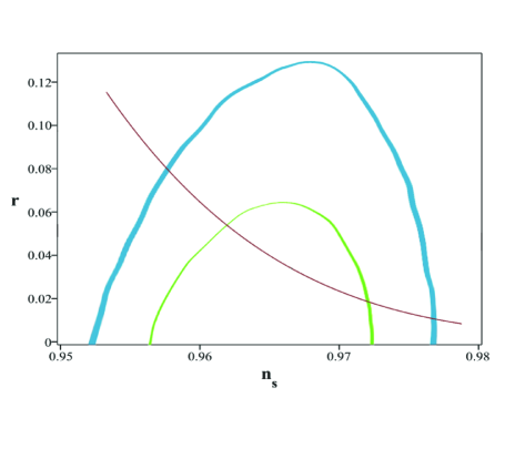
Figure 1: Tensor-to-scalar ratio versus the scalar spectral index in the background of Planck2015 TT,TE and EE+lowP data.

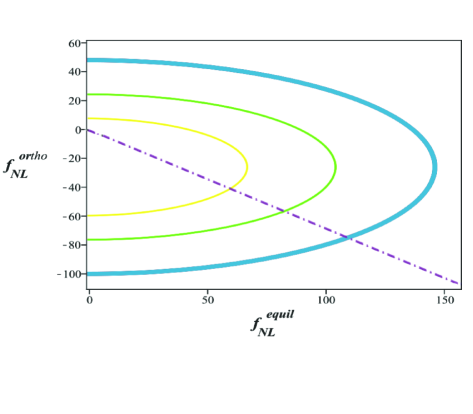
Figure 2: The amplitude of the orthogonal configuration versus the amplitude of the equilateral configuration of non-Gaussianity in the background of Planck2015 TTT, EEE, TTE and EET data.

6 Summary and Conclusion

We studied an extended model of single field inflation where the inflaton and its derivatives are coupled to the background geometry. By focusing on the third order action and nonlinear perturbations we obtained observables of cosmological inflation, such as tensor-to-scalar ratio and the amplitudes of non-Gaussianities in this extended setup. By confronting the model’s outcomes with observational data from Planck2015, we were able to constraint parameter space of the model. By adopting a quartic potential with $V(\phi)=\frac{1}{4}\lambda\phi^{4}$, restricting the model to realize observationally viable spectral index (or tensor-to-scalar ratio) imposes the constraint on coupling $\lambda$ as $0.013<\lambda<0.095$. Also restricting the amplitude of equilateral amplitude of non-Gaussianity to the observationally supported value of $-147<f^{equi}_{NL}<143$, results in the constraint $\lambda<0.1$ in appropriate units.

Acknowledgement
The work of K. Nozari has been supported financially by Research Institute for Astronomy and Astrophysics of Maragha (RIAAM) under research project number 1/5750-1.

References

• [1] V. F. Mukhanov and G. V. Chibisov, JETP Lett. 33, 532 (1981).
• [2] A. Guth, Phys. Rev. D 23 (1981) 347.
• [3] A. Albrecht and P. Steinhard, Phys. Rev. D 48 (1982) 1220.
• [4] A. D. Linde, Phys. Lett. B 108 (1982) 389.
• [5] A. A. Starobinsky, Phys. Lett. B 117 (1982) 175.
• [6] J. E. Lidsey et. al., Rev. Mod. Phys. 69 (1997) 373.
• [7] A. Liddle and D. Lyth, Cambridge University Press, 2000.
• [8] E. Komatsu et al., Astrophys. J. Suppl. 192, 18 (2011).
• [9] J. Martin, [arXiv:1502.05733]. See also J. Martin, [arXiv:1312.3720].
• [10] J. M. Maldacena, J. High Energy Phys. 05 (2003) 013.
• [11] P. A. R. Ade et al., [arXiv:1502.02114].
• [12] P. A. R. Ade et al., [arXiv:1502.01589].
• [13] P. A. R. Ade et al., [arXiv:1502.01592].
• [14] D. Baumann, [arXiv:0907.5424].
• [15] Y. Wang, [arXiv:1303.1523].
• [16] A. De Felice and S. Tsujikawa, Phys. Rev. D 84 (2011) 083504.
• [17] A. De Felice and S. Tsujikawa, JCAP 1104 (2011) 029.
• [18] A. De Felice and S. Tsujikawa, JCAP 03 (2013) 030.
• [19] Q.-G. Huang and Y. Wang, JCAP 06 (2013) 035.
• [20] V. Faraoni, Phys. Rev. D 62 (2000) 023504.
• [21] T. Futamase and K. I. Maeda, Phys. Rev. D 39 (1989) 399.
• [22] D. S. Salopek, J. R. Bond and J. M. Bardeen, Phys. Rev. D 40 (1989) 1753.
• [23] R. Fakir and W. G. Unruh, Phys. Rev. D 41 (1990) 1783.
• [24] N. Makino and M. Sasaki, Prog. Theor. Phys. 86 (1991) 103.
• [25] J. Hwang and H. Noh, Phys. Rev. D 60 (1999) 123001.
• [26] S. Tsujikawa and H. Yajima, Phys. Rev. D 62 (2000) 123512.
• [27] C. Pallis and N. Toumbas, JCAP 1102 (2011) 019.
• [28] K. Nozari and S. Shafizadeh, Phys. Scripta 82 (2010) 015901.
• [29] C. P. Burgess, H. M. Lee and M. Trott, JHEP 0909 (2009) 103.
• [30] J. L. F. Barbon and J. R. Espinosa, Phys. Rev. D 79 (2009) 081302.
• [31] C. P. Burgess, H. M. Lee, and M. Trott, JHEP 07 (2010) 007.
• [32] L. Amendola, Phys. Lett. B 301 (1993) 175.
• [33] C. Germani and A. Kehagias, Phys. Rev. Lett. 105 (2010) 011302, see also A. Escriva and C. Germani, Phys. Rev. D 95, 123526 (2017) for more recent paper on this issue.
• [34] S. Tsujikawa, Phys. Rev. D 85 (2012) 083518.
• [35] H. M. Sadjadi and P. Goodarzi, JCAP 02 (2013) 038.
• [36] E. N. Saridakis and S. V. Sushkov, Phys. Rev. D 81 (083510) 2010.
• [37] R. L. Arnowitt, S. Deser and C. W. Misner, Phys. Rev. 117 (1960) 1595.
• [38] V. F. Mukhanov, H. A. Feldman, R. H. Brandenberger,Physics Reports 215 (1992) 203.
• [39] C. Cheung, P. Creminelli, A. L. Fitzpatrick, J. Kaplan and L. Senatore, JHEP 0803 (2008) 014.
• [40] D. Seery and J. E. Lidsey, JCAP 0506 (2005) 003.
• [41] J. Hwang and H. Noh, Phys.Rev. D 54 (1996) 1460.
• [42] H. Noh and J. Hwang, Phys. Lett. B 515 (2001) 231.
• [43] R. Myrzakulov, L. Sebastiani and S. Vagnozzi, Eur. Phys. J. C 75 (2015) 444
• [44] D. Babich, P. Creminelli and M. Zaldarriaga, JCAP 08 (2004) 009.
• [45] L. Senatore, K. M. Smith and M. Zaldarriaga, JCAP 1 (2010) 28.
• [46] J. R. Fergusson and E. P. S. Shellard, Phys. Rev. D 80 (2009) 043510.
• [47] A. De Felice and S. Tsujikawa, JCAP 03 (2013) 030.
• [48] C. T. Byrnes, [arXiv:1411.7002].
• [49] X. Chen, M. X. Huang, S. Kachru and G. Shiu, JCAP 0701 (2007) 002.