Angle and magnitude decorrelation in the factorization breaking of collective flow

Abstract

The collective harmonic flow in heavy-ion collisions correlates particles at all transverse momenta to be emitted preferably some directions. The factorization breaking coefficient measures the small decorrelation of the flow harmonics at two different transverse momenta. Using the hydrodynamic model I study in details the decorrelation of the harmonic flow due to the flow angle and the flow magnitude decorrelation at two transverse momenta. The effect can be seen in experiment measuring factorization breaking coefficients for the square of the harmonic flow vector at two transverse momenta. The hydrodynamic model predicts that the decorrelation of the flow magnitudes is about one half of the decorrelation of the overall flow (combining flow angle and flow magnitude decorrelations). These results are consistent with the principal component analysis of correlators of flow vectors squared.

I Introduction

The collective expansion of dense matter created in relativistic nuclear collisions creates strong correlation between emitted particles Heinz:2013th ; Gale:2013da ; Ollitrault:2010tn . The azimuthal asymmetry of the collective flow gives rise to an asymmetry of particle spectra

$$\frac{dN}{d\phi} \propto 1+v_{2}\cos\left(2(\phi-\Psi_{2})\right)$$

$$+ v_{3}\cos\left(3(\phi-\Psi_{3})\right)+\dots\ .$$

In the above equation the elliptic $v_{2}$ and triangular $v_{3}$ flows and the flow angles $\Psi_{n}$ are collective parameters of the spectra that fluctuate from event to event. The harmonic flow coefficients can be extracted from two (or higher) particle correlations. The study of the flow coefficients in heavy-ion collisions at different centralities is a way to extract the properties of the expanding medium, in particular the value of shear viscosity.

The collective parameters can depend on particle transverse momentum or pseudorapidity $v_{n}(p_{\perp},\eta)$, $\Psi_{n}(p_{\perp},\eta)$. Using correlations of two particles at different pseudorapidities Bozek:2010vz or different transverse momenta Gardim:2012im the decorrelation of the flow parameters at different $p_{\perp}$ or $\eta$ can be observed. The phenomenon is known as flow factorization breaking in pseudorapidity or transverse momentum. It has been measured experimentally Acharya:2017ino ; Aad:2014lta ; Khachatryan:2015oea ; Aaboud:2017tql and calculated in models Gardim:2012im ; Heinz:2013bua ; Kozlov:2014fqa ; Lin:2004en ; Pang:2015zrq ; Xiao:2015dma . It is found that the factorization breaking coefficient is sensitive to fluctuations in the initial state. The initial fluctuations are transformed by the collective expansion into a small decorrelation of flow parameters at two transverse momenta or pseudorapidities. The predicted decorrelation is not strongly dependent on the viscosity.

Factorization breaking coefficients from two-particle correlations measure the overall flow decorrelation, which is a combined effect of the decorrelation of the collective flow magnitudes $v_{n}(p_{\perp},\eta)$ and of the decorrelation of the flow angles $\Psi_{n}(p_{\perp},\eta)$ at two different transverses momenta or rapidities. By using $4$-particle correlators the flow angle decorrelation and the overall flow decorrelation in pseudorapidity can be measured separately Aaboud:2017tql ; Jia:2017kdq . Experimental data and hydrodynamic model simulations Bozek:2017qir ; Wu:2018cpc show that the angle decorrelation accounts for only a part of the overall flow decorrelation in pseudorapidity.

In this paper the analogous effect is studied for the harmonic flow decorrelation in transverse momentum. In the hydrodynamic model the flow angle and the flow magnitude decorrelations at different transverse momenta are studied separately and compared to the overall flow decorrelation (Sect. III). Model calculations show that the flow decorrelation in a particular event is correlated to the flow magnitude in the same event. This could be measured experimentally by using correlators weighed with different powers of $v_{n}$ (Sect. IV). In order to measure the flow angle or flow magnitude decorrelations separately $4$-particle correlations must be used. Unlike for the decorrelation in pseudorapidity, where the flow angle decorrelation can be estimated, for the factorization breaking in transverses momentum a measure of the flow magnitude decorrelation can be naturally defined (Sect. VI). The flow magnitude decorrelation accounts for about one half of the overall flow decorrelation at two different transverse momenta. The findings are consistent with the principal component analysis of correlation matrices of higher powers of harmonic flow (Sect. VII).

II Model

I use 3+1 dimensional relativistic viscous hydrodynamics with Monte Carlo Glauber model initial conditions  Schenke:2010rr ; Bozek:2011ua to model Pb+Pb collisions at $\sqrt{s_{NN}}=5.02$ TeV. The initial entropy deposition in the transverse plane is given as a sum of contributions from $N_{p}$ participant nucleons

$$s(x,y)=\sum_{i=1}^{N_{p}}g_{i}(x,y)\$$ (1)

(the form of the initial distribution in the longitudinal direction is skipped here for simplicity, it follows the parametrization given in Ref. Bozek:2011ua ). Each nucleon gives a Gaussian-smeared contribution

$$g_{i}(x,y) = \kappa\left((1-\alpha)+\alpha c_{i}\right)$$ (2)

$$\exp\left(-\frac{(x-x_{i})^{2}+(y-y_{i})^{2}}{2\sigma^{2}}\right),$$

where $c_{i}$ is the number of collisions for nucleon $i$ at position $(x_{i},y_{i})$ and $\kappa$ is adjusted to reproduce the charged particle density in pseudorapidity. For Pb+Pb collisions at $\sqrt{s_{NN}}=5.02$ TeV $\alpha=0.1$ is taken to describe the centrality dependence of the charged particle density. At the freeze-out temperature $150$ MeV statistical emission of hadrons takes place Chojnacki:2011hb .

For each hydrodynamic event I generate $150$ or $600$ events for centralities $0-5$% and $30-40$%. For each hydrodynamic event the collective flow is calculated by combining these events. This procedure reduces statistical errors and non-flow contributions in multiparticle correlators Bozek:2017thv . The event-by-event reconstruction of the flow vectors in the model allows to calculate the flow angle or flow magnitude decorrelation separately. The flow correlations are analyzed in the transverse momentum range $p_{\perp}\in[0.3,3.0]$ GeV. The $p_{\perp}$ range is divided into bins of unequal width, but of equal mean particle multiplicity in each bin Bozek:2017thv . This choice guarantees that the statistical errors for the all the elements of correlators in two $p_{\perp}$ bins are similar.

III Flow angle and flow magnitude decorrelation

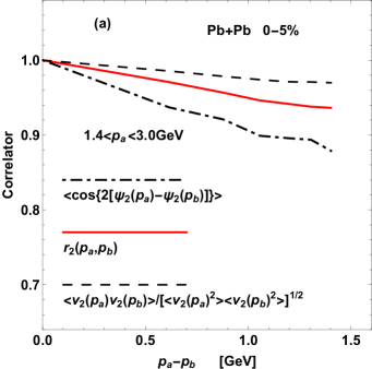
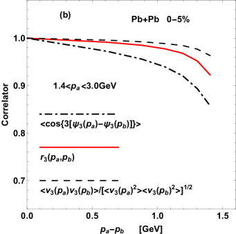
Figure 1: Correlator for the flow angle from Eq. (6) (dot-dashed line), for the flow magnitude from Eq. (7) (dashed line), and for the harmonic flow from Eq. (3) (solid line) for two bins in transverse momentum. Panels (a) and (b) show the results for the second- and third-order harmonic flow, respectively. Pb+Pb collisions at $\sqrt{s_{NN}}=5.02$ TeV for centrality 0-5%.

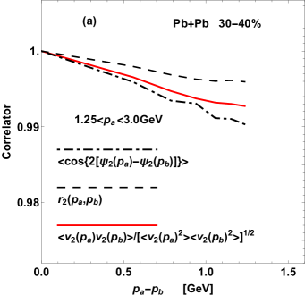
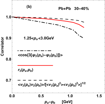
Figure 2: Same as Fig. 1 but for centrality 30-40%.

The decorrelation of harmonic flow at two different transverse momenta $p_{a}$ and $p_{b}$ is measured using the factorization breaking coefficient Gardim:2012im

$$r_{n}(p_{a},p_{b})=\frac{\langle q_{n}(p_{a})q_{n}^{\star}(p_{b})\rangle}{\sqrt{\langle v_{n}(p_{a})^{2}\rangle\langle v_{n}(p_{p})^{2}\rangle}}\ ,$$ (3)

where

$$q_{n}(p)=\frac{1}{N}\sum_{j}e^{in\phi_{j}}=v_{n}(p)e^{in\Psi_{n}(p)}$$ (4)

is the $q$ vector of the n-th order harmonic flow calculated from the azimuthal angles $\phi_{j}$ of $N$ particles in the bin at transverse momentum $p$ and $\langle\dots\rangle$ denotes the average over events. The n-th harmonic at transverse momentum $p$ can be written as

$$\langle v_{n}(p)^{2}\rangle=\langle q_{n}(p)q_{n}^{\star}(p)\rangle=\frac{1}{N(N-1)}\sum_{j\neq k}e^{in(\phi_{j}-i\phi_{k})}\ .$$ (5)

In this paper I use the convention that selfcorrelation terms are dropped from sums over particles in the same bin.

For flow dominated correlations between emitted particles the factorization breaking coefficient $r_{n}$ measures the correlation coefficient of the flow vectors $q_{n}$ at different transverse momenta. In that case $r_{n}(p_{a},p_{b})\leq 1$ Gardim:2012im . The value $r_{n}(p_{a},p_{b})<1$ means that the harmonic flow at the transverse momenta $p_{a}$ and $p_{b}$ is partially decorrelated. This decorrelation can be due to a flow magnitude or a flow angle decorrelation Jia:2014vja . Flow angle decorrelation means that event-by-event differences in the effective flow angles $\Psi_{n}(p_{a})$ and $\Psi_{n}(p_{b})$ at the two transverse momenta appear. The flow angle difference $\Psi(p_{a})-\Psi_{n}(p_{b})$ contributes a factor $\cos\left\{n\left[\Psi_{n}(p_{a})-\Psi_{n}(p_{b})\right]\right\}$ in the numerator of of the factorization breaking coefficient $r_{n}(p_{a},p_{b})$. The decorrelation of the harmonic flow angles is defined as

$$\langle\cos\left\{n\left[\Psi_{n}(p_{a})-\Psi_{n}(p_{b})\right]\right\}\rangle\ .$$ (6)

The decorrelation of the magnitude of the harmonic flow at two transverse momenta can be defined as

$$\frac{\langle v_{n}(p_{a})v_{n}(p_{b})\rangle}{\sqrt{\langle v_{n}(p_{a})^{2}\rangle\langle v_{n}(p_{p})^{2}\rangle}}\ .$$ (7)

Please note that the angle (6) and magnitude (7) decorrelations cannot be calculated from experimental data. On the other hand, these quantities can be estimated in the hydrodynamic model integrating over the particle distributions in momenta, instead of a summation over particles in an event. In practice this integration is performed using a Monte Carlo method by generating a large number of particles at the freeze-out hypersurface, as described in Sect. II. If the angle and magnitude decorrelation factorize, on has

$$r_{n}(p_{a},p_{b})\simeq$$

$$\frac{\langle v_{n}(p_{a})v_{n}(p_{b})\rangle}{\sqrt{\langle v_{n}(p_{a})^{2}\rangle\langle v_{n}(p_{p})^{2}\rangle}}\langle\cos\left\{n\left[\Psi_{n}(p_{a})-\Psi_{n}(p_{b})\right]\right\}\rangle\ .$$ (8)

In Figs. 1 and 2 are compared the factorization breaking coefficients $r_{n}(p_{a},p_{b})$, the angle decorrelation (6), and the magnitude decorrelation (7). The factorization breaking coefficient is not a simple product of the angle and magnitude decorrelations as in Eq. 8. In fact, an inverted hierarchy of decorrelations appears. The angle decorrelation (6) is stronger than the flow decorrelation given by the factorization breaking coefficient $r_{2}$. The reason for the inverted hierarchy is that the three averages in Eq. 8 are weighted with different powers of $v_{n}$ Bozek:2017qir . The decorrelation of the flow angles is anticorrelated with the overall magnitude of the flow in an event. Therefore the average (6), that is weighted with a zeroth power of $v_{n}$, gives a larger deviation from $1$, i.e. a stronger decorrelation than the other two averages in Figs. 1 and 2.

IV Correlation of the overall flow magnitude and of the flow decorrelation

On an event-by-event basis an anti-correlation occurs between the magnitude of the flow $v_{n}^{2}$ in the event and the factorization breaking coefficient. In events with a larger flow the the decorrelation is smaller ($r_{n}$ is bigger, closer to $1$). This effect has been observed in model calculations for the decorrelation in pseudorapidity Bozek:2017qir . The same effect can be evidenced for the decorrelation of flow in transverse momentum.

Experimentally factorization breaking coefficients weighted with different powers of $v_{n}$ can be defined

$$r_{n|n;1}^{n;2k}(p_{a},p_{b})=\frac{\langle v_{n}^{2k}q_{n}(p_{a})q_{n}^{\star}(p_{b})\rangle}{\sqrt{\langle v_{n}^{2k}v_{n}(p_{a})^{2}\rangle\langle v_{n}^{2k}v_{n}(p_{p})^{2}\rangle}}\ .$$ (9)

For $k=0$ the above formula reduces to the standard factorization breaking coefficient $r_{n}(p_{a},p_{b})$. The correlators in the numerator and denominator of Eq. 9 involve summation over $2+2k$ particles. Self-correlations must be subtracted in the summation. In experiment non-flow effects can be reduced using rapidity gaps.

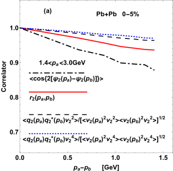
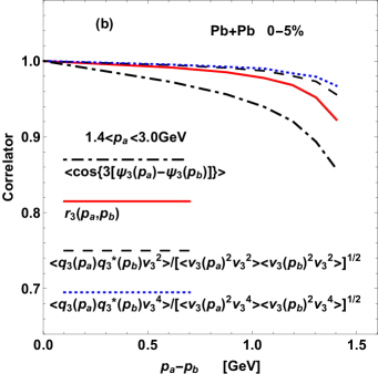
Figure 3: Correlator of the flow (solid line), of the flow weighted with $v_{n}^{2}$ (dashed line), and of the flow weighted with $v_{n}^{4}$ (dotted line) at two different transverse momenta. The dash-dotted line represent the correlator for the flow angle (6). Panels (a) and (b) show the results for the second- and third-order harmonic flow, respectively. Pb+Pb collisions at $\sqrt{s_{NN}}=5.02$ TeV for centrality 0-5%.

In Figs. 3 and 4 are shown the correlators $r_{n|n;1}^{n;2k}(p_{a},p_{b})$ for $k=0,1,2$. The flow magnitude in the weighting factor $v_{n}^{2k}$ corresponds to the integrated flow in $p_{\perp}\in[0.3,3.0]$ Gev. For correlators with higher powers of the weighting factor $v_{n}^{2k}$ the decorrelation is weaker. This prediction could be tested in experiment in order to evidence the relation between the overall flow magnitude and the flow decorrelation in transverse momentum. The angle decorrelation (6) is shown in Figs. 3 and 4 as well (dash-dotted lines). This quantity give the strongest decorrelation, as it corresponds to having effectively a weighting factor $v_{n}^{-2}$. This last correlator can be estimated in the model but not in the experiment.

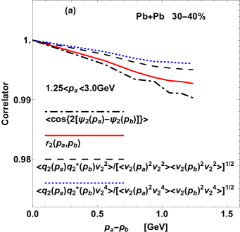
Figure 4: Same as Fig. 3 but for centrality 30-40%.

V Higher order flow correlators

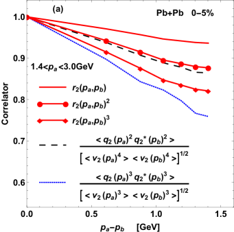
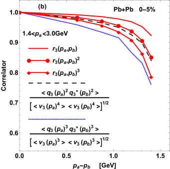
Figure 5: Correlator of the flow (solid line), of the flow squared (dashed line), and of the flow to power $3$ (dotted line) at two different transverse momenta. Solid lines with symbols represent second and third powers of the standard flow correlator $r_{2}$. Panels (a) and (b) show the results for the second- and third-order harmonic flow, respectively. Pb+Pb collisions at $\sqrt{s_{NN}}=5.02$ TeV for centrality 0-5%.

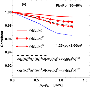
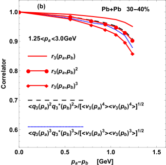
Figure 6: Same as Fig. 5 but for centrality 30-40%.

Correlators of higher powers of the flow in two different pseudorapidity bins have been measured experimentally Aaboud:2017tql and calculated in the hydrodynamic model Bozek:2017qir ; Wu:2018cpc . The simplest higher order correlators involve higher powers of the $q$ vectors

$$r_{n|n;k}(p_{a},p_{b})=\frac{\langle q_{n}(p_{a})^{k}q_{n}^{\star}(p_{b})^{k}\rangle}{\sqrt{\langle v_{n}(p_{a})^{2k}\rangle\langle v_{n}(p_{p})^{2k}\rangle}}\ .$$ (10)

For $k=1$ one recovers the factorization breaking coefficient (3) $r_{n|n;1}(p_{a},p_{b})=r_{n}(p_{a},p_{b})$.

Correlators involving higher powers of the flow vector yield stronger decorrelation, $r_{n|n;3}(p_{a},p_{b})<r_{n|n;2}(p_{a},p_{b})<r_{n|n;1}(p_{a},p_{b})$ (Figs. 5 and 6). Factorization breaking coefficients for higher powers of flow vectors do not factorize into powers of the basic factorization coefficient

$$r_{n|n;k}(p_{a},p_{b})\neq r_{n}(p_{a},p_{b})^{k}\ \ .$$ (11)

VI Measuring flow magnitude factorization breaking

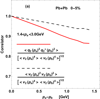
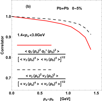
Figure 7: Correlator for the flow squared (solid line) and for the flow magnitude squared (dashed line). Panels (a) and (b) show the results for the second- and third-order harmonic flow, respectively. Pb+Pb collisions at $\sqrt{s_{NN}}=5.02$ TeV for centrality 0-5%.

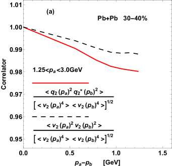
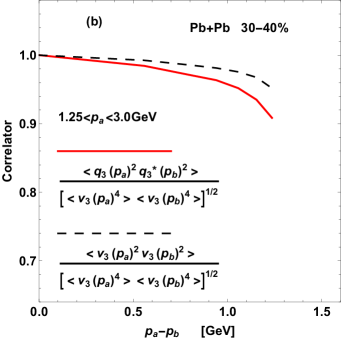
Figure 8: Same as Fig. 7 but for centrality 30-40%.

The angle and magnitude factorization breaking coefficients discussed in Sect. III given by Eqs. 6 and 7 cannot be measured experimentally. The angle decorrelation in pseudorapidity can been measured separately using a $4$-bin correlator Aaboud:2017tql ; Jia:2017kdq . That correlator involves $4$ $q_{n}$ vectors and should be compared to the correlator of the square of the $q_{n}$ vectors in two bins. It was found that the flow decorrelation (involving flow magnitude and flow angle decorrelation combined) is twice as strong than the flow angle decorrelation alone, both in experiment Aaboud:2017tql and in model calculations Bozek:2017qir ; Wu:2018cpc .

The situation is slightly different for the decorrelation of the harmonic flow in transverse momentum. One can define a correlator measuring the decorrelation of the flow magnitude squared

$$r_{n}^{v_{n}^{2}}(p_{a},p_{b})=\frac{\langle v_{n}(p_{a})^{2}v_{n}(p_{b})^{2}\rangle}{\sqrt{\langle v_{n}(p_{a})^{4}\rangle\langle v_{n}(p_{b})^{4}\rangle}}\ .$$ (12)

The above correlator can be compared to the correlator of flow vector squared $r_{n|n;2}(p_{a},p_{b})$ (10). Both correlators $r_{n}^{v_{n}^{2}}(p_{a},p_{b})$ and $r_{n|n;2}(p_{a},p_{b})$ involve averages of $4$ $q_{n}$ vectors and both correlators can be measured in the experiment. The first one measures the flow magnitude decorrelation alone, while the second one measures the flow magnitude and flow angle decorrelations combined.

The predictions for the two correlators for two centralities are presented in Figs. 7 and 8. The decorrelation of the flow magnitude is significantly smaller than the flow decorrelation. Both for the elliptic and triangular flows, I find that the flow magnitude decorrelation accounts for roughly half of the total flow decorrelation

$$1-r_{n}^{v_{n}^{2}}(p_{a},p_{b})\simeq\frac{1}{2}\left(1-r_{n|n;2}(p_{a},p_{b})\right)\ \ .$$ (13)

VII Principal component analysis

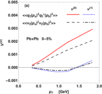
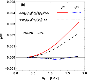
Figure 9: Leading (solid line) and subleading (dashed line) eigenmodes of the correlation matrix of the square of the harmonic flow at two transverse momenta. The dotted and dash-dotted lines denote the leading and subleading eigenmodes for the correlation matrix of the square of the magnitude of the harmonic flow. Panel (a) and (b) present results for the elliptic and triangular flow respectively. Pb+Pb collisions at $\sqrt{s_{NN}}=5.02$ TeV for centrality 0-5%.

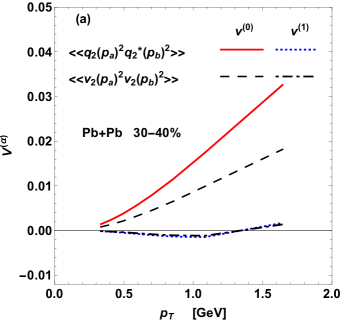
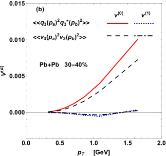
Figure 10: Same as Fig. 9 but for centrality 30-40%.

The correlation matrix of the harmonic flow can be decomposed into its principal components Bhalerao:2014mua

$$\langle\langle q_{n}(p_{a})q_{n}^{\star}(p_{b})\rangle\rangle=\langle q_{n}(p_{a})q_{n}^{\star}(p_{b})\rangle-\langle q_{n}(p_{a})\rangle\langle q_{n}^{\star}(p_{b})\rangle$$

$$=\langle q_{n}(p_{a})q_{n}^{\star}(p_{b})\rangle=$$

$$v_{n}^{(0)}(p_{a})v_{n}^{(0)}(p_{b})+v_{n}^{(1)}(p_{a})v_{n}^{(1)}(p_{b})+\dots\ ,$$ (14)

where the leading eigenmode is $v_{n}^{(0)}(p_{a})\simeq\sqrt{\langle v_{n}(p_{a})^{2}\rangle}$. If the subleading modes can be neglected the correlation matrix factorizes

$$\langle\langle q_{n}(p_{a})q_{n}^{\star}(p_{b})\rangle\rangle\simeq\sqrt{\langle v_{n}(p_{a})^{2}\rangle\langle v_{n}(p_{b})^{2}\rangle}\ .$$ (15)

The factorization breaking coefficient can be written as Bhalerao:2014mua

$$r_{n}(p_{a},p_{b})=1-\frac{1}{2}\left|\frac{v_{n}^{(1)}(p_{a})}{v_{n}^{(0)}(p_{a})}-\frac{v_{n}^{(1)}(p_{b})}{v_{n}^{(0)}(p_{b})}\right|^{2}\ .$$ (16)

The principal component decomposition of the flow correlation matrix (14) carries the information about the flow factorization breaking.

The flow magnitude decorrelation discussed in the previous section involves a correlation of higher powers of the flow vectors. One can define the decomposition

$$\langle v_{n}^{2}(p_{a})v_{n}^{2}(p_{b})\rangle=$$

$$v_{v_{n}^{2}}^{(0)}(p_{a})v_{v_{n}^{2}}^{(0)}(p_{b})+v_{v_{n}^{2}}^{(1)}(p_{a})v_{v_{n}^{2}}^{(1)}(p_{b})+\dots\ .$$ (17)

The flow magnitude factorization breaking is

$$r_{n}^{v_{n}^{2}}(p_{a},p_{b})=1-\frac{1}{2}\left|\frac{v_{v_{n}^{2}}^{(1)}(p_{a})}{v_{v_{n}^{2}}^{(0)}(p_{a})}-\frac{v_{v_{n}^{2}}^{(1)}(p_{b})}{v_{v_{n}^{2}}^{(0)}(p_{b})}\right|^{2}\ .$$ (18)

Please note that the correlator $\langle v_{n}^{2}(p_{a})v_{n}^{2}(p_{b})\rangle$ is not a correlation matrix. The proper correlation matrix for $v_{n}^{2}$ is

$$\langle\langle v_{n}^{2}(p_{a})v_{n}^{2}(p_{b})\rangle\rangle=$$

$$\langle v_{n}^{2}(p_{a})v_{n}^{2}(p_{b})\rangle-\langle v_{n}^{2}(p_{a})\rangle\langle v_{n}^{2}(p_{b})\rangle=$$

$$\tilde{v}_{v_{n}^{2}}^{(0)}(p_{a})\tilde{v}_{v_{n}^{2}}^{(0)}(p_{b})+\tilde{v}_{v_{n}^{2}}^{(1)}(p_{a})\tilde{v}_{v_{n}^{2}}^{(1)}(p_{b})+\dots\ .$$ (19)

The eigenmode decompositions of the two matrices (17) and (19) are related with

$$\tilde{v}_{v_{n}^{2}}^{(1)}(p_{a})\simeq{v}_{v_{n}^{2}}^{(1)}(p_{a})\ \ .$$ (20)

On the other hand, the dominance of the leading mode gives

$$v_{n}^{(0)}(p_{a})\simeq v_{v_{n}^{2}}^{(0)}(p_{a})\ .$$ (21)

In Figs. 9 and 10 are shown the eigenmodes for the matrices $\langle\langle q_{n}(p_{a})q_{n}^{\star}(p_{b})\rangle\rangle$ and $\langle\langle v_{n}^{2}(p_{a})v_{n}^{2}(p_{b})\rangle\rangle$ (due to the relations (20) and (21) the eigenmodes for $\langle v_{n}^{2}(p_{a})v_{n}^{2}(p_{b})\rangle$ overlap with the curves on the plot). The subleading mode is much smaller than the leading one, which is consistent with small factorization breaking. The subleading modes are similar in shape

$$v_{v_{n}^{2}}^{(1}(p_{a})\simeq\tilde{v}_{v_{n}^{2}}^{(1)}(p_{a})\simeq 0.7v_{n}^{(1)}(p_{a})\ ,$$ (22)

which leads to a similar shape of the factorization breaking of the flow and of the flow magnitude (Eq. 13).

VIII Summary

The factorization breaking of harmonic flow at two different transverse momenta is studied in the hydrodynamic model. In the model the decorrelation of the flow angle and of the flow magnitude is calculated. The flow angle decorrelation is strongly correlated with the overall flow magnitude in an event. A way to measure this correlation in experiment is discussed, and predictions are made within the hydrodynamic model.

The separate decorrelation of the flow angle and flow magnitude observed in the model cannot be measured in experiment using two-particle correlation. The flow magnitude decorrelation could be measured in experiment using a $4$-particle correlations. The hydrodynamic model with Monte Carlo Glauber initial conditions predicts that the flow magnitude decorrelation is about one half of the overall flow decorrelation. The difference in the flow factorization breaking or the flow magnitude factorization breaking can be studied using the principal component analysis of the relevant $4$-particle correlation matrices. The hierarchy of the eigenmodes in the principal component analysis is consistent with results on factorization breaking.

References

- (1) U. Heinz and R. Snellings, Ann.Rev.Nucl.Part.Sci. 63, 123 (2013)
- (2) C. Gale, S. Jeon, and B. Schenke, Int.J.Mod.Phys. A28, 1340011 (2013)
- (3) J.-Y. Ollitrault, J. Phys. Conf. Ser. 312, 012002 (2011)
- (4) P. Bożek, W. Broniowski, and J. Moreira, Phys. Rev. C83, 034911 (2011)
- (5) F. G. Gardim, F. Grassi, M. Luzum, and J.-Y. Ollitrault, Phys.Rev. C87, 031901 (2013)
- (6) S. Acharya et al. (ALICE Collaboration), JHEP 09, 032 (2017)
- (7) G. Aad et al. (ATLAS Collaboration), Phys.Rev. C90, 044906 (2014)
- (8) V. Khachatryan et al. (CMS Collaboration), Phys. Rev. C92, 034911 (2015)
- (9) M. Aaboud et al. (ATLAS), Eur. Phys. J. C78, 142 (2018)
- (10) U. Heinz, Z. Qiu, and C. Shen, Phys.Rev. C87, 034913 (2013)
- (11) I. Kozlov, M. Luzum, G. Denicol, S. Jeon, and C. Gale(2014), arXiv:1405.3976 [nucl-th]
- (12) Z.-W. Lin, C. M. Ko, B.-A. Li, B. Zhang, and S. Pal, Phys. Rev. C72, 064901 (2005)
- (13) L.-G. Pang, H. Petersen, G.-Y. Qin, V. Roy, and X.-N. Wang, Eur. Phys. J. A52, 97 (2016)
- (14) K. Xiao, L. Yi, F. Liu, and F. Wang, Phys. Rev. C94, 024905 (2016)
- (15) J. Jia, P. Huo, G. Ma, and M. Nie, J. Phys. G44, 075106 (2017)
- (16) P. Bożek and W. Broniowski, Phys. Rev. C97, 034913 (2018)
- (17) X.-Y. Wu, L.-G. Pang, G.-Y. Qin, and X.-N. Wang(2018), arXiv:1805.03762 [nucl-th]
- (18) B. Schenke, S. Jeon, and C. Gale, Phys. Rev. Lett. 106, 042301 (2011)
- (19) P. Bożek, Phys. Rev. C85, 034901 (2012)
- (20) M. Chojnacki, A. Kisiel, W. Florkowski, and W. Broniowski, Comput. Phys. Commun. 183, 746 (2012)
- (21) P. Bożek, Phys. Rev. C97, 034905 (2018)
- (22) J. Jia and P. Huo, Phys.Rev. C90, 034905 (2014)
- (23) R. S. Bhalerao, J.-Y. Ollitrault, S. Pal, and D. Teaney, Phys. Rev. Lett. 114, 152301 (2015)