Characterization of Electric Fields for Perfect Conductivity Problems in 3D
Abstract.
In composite materials, the inclusions are frequently spaced very closely. The electric field concentrated in the narrow regions between two adjacent perfectly conducting inclusions will always become arbitrarily large. In this paper, we establish an asymptotic formula of the electric field in the zone between two spherical inclusions with different radii in three dimensions. An explicit blowup factor relying on radii is obtained, which also involves the digamma function and Euler-Mascheroni constant, and so the role of inclusions’ radii played in such blowup analysis is identified.
1. Introduction and main results
In this paper, we investigate the blowup phenomena that occur in composite materials consisting of a finite conductivity matrix and perfectly conducting inhomogeneities close to touching and derive the asymptotic formula of the electric field in the narrow region between two perfectly conducting inclusions in three dimensions. For two spherical inclusions with different radii, we obtain an explicit blowup factor involving the digamma function and Euler-Mascheroni constant and reveal the role of radii of inclusions played in such blowup analysis.
This problem was initiated by Babuska et al [8] in the study of fiber-reinforced composite material, where one has to estimate the magnitude of local fields in the zone of high stress field concentration. It can be modeled by a class of divergence form second-order elliptic equations with piecewise constant coefficients, given by for inside the inclusions, and in the matrix. This model has attracted considerable attention because it can describe various physical phenomena, including electrical conductivity, thermal conduction, anti-plane elasticity, and even flow in porous media. For the sake of definiteness, this paper uses the electrical conductivity language, where describes an electric field.
There have been much important progress made on the gradient estimates of the solutions to such elliptic equations since the numerical analysis was studied in [8]. For the case when the conductivity stays away from 0 and , Bonnetier and Vogelius [16] first proved that is bounded for two touching disks and in two dimensions. Moreover, they pointed out that the bound depends on the value of conductivity. Li and Vogelius [32] extended the result to general divergence form second-order elliptic equations with piecewise smooth coefficients and they proved that remains uniformly bounded with respect to the distance between inclusions of arbitrary smooth shape in all dimensions. Li and Nirenberg [31] extended this result to elliptic systems including systems of linear elasticity, which is assumed in [8]. The estimates in [31] and [32] depend on the ellipticity of the coefficients. If ellipticity constants are allowed to be deteriorate, the situation is very different. It was shown in various papers, see for example Budiansky and Carrier [18] and Markenscoff [38], that when the -norm of generally becomes unbounded as the distance between inclusions tends to zero. The rate at which the -norm of the gradient of a special solution blows up was shown in [18] to be in two dimensions.
In this paper, we consider the perfect conductivity problem, where . It was proved by Ammari, Kang and Lim in [7] and Ammari et al. in [5] that when and are disks in , the blowup rate of is as goes to zero; with the lower bound given in [7] and the upper bound given in [5]. This result was extended by Yun [39, 40] and Bao, Li and Yin [9] to strictly convex subdomains and in . In three dimensions and higher dimensions, the blowup rate of turns out to be and , respectively; see [9, 35]. For related works on elliptic equations and systems arising from the study of composite materials, see [1, 3, 4, 6, 10, 12, 13, 11, 14, 15, 17, 19, 20, 22, 23, 24, 27, 29, 30, 33, 35, 36, 37, 41, 42] and the references therein.
The results mentioned above are estimates of from above and below, namely,
| (1.1) |
for some positive constants and , where , , , if , , , respectively, and shows that the electric filed may blow up in the narrow regions between inclusions.
The interest of this paper lies in further establishing the asymptotic formula of in the narrow zone of electric field concentration. In dimension two, Kang, Lim and Yun [25] obtained a complete characterization of the singular behavior of when inclusions are disks. Let and be disks in of radii and , respectively, and let be the reflection with respect to , . Then the combined reflections and have unique fixed points, say and . Let
| (1.2) |
It has been proved that the solution to (1.4) can be expressed as
| (1.3) |
where c is the middle point of the shortest line segment connecting and , n is the unit vector in the direction of , and is bounded independently of on any bounded subset of . So the singular behavior of is completely characterized by . Ammari et al. [2] extended the characterization (1.3) to the case when inclusions are strictly convex domains in by using disks osculating to convex domains. It is worth mentioning that stress concentration factor was derived by Gorb in [21], and by Gorb and Novikov in [22] for the -Laplacian.
Compared with the known results in dimension two, the situation becomes more complicated in dimension three. Although the singular function can be founded, it is of form of series, see (2.9) below, rather than a function like (1.2). Recently, for a special case that two inclusions with the same radii , an asymptotic formula of was obtained by Kang, Lim and Yun in [26], where the symmetry of the domain makes the computation easy to handle. However, for the general case that , the symmetry is broken and the computation becomes involved. It is not obvious to generalize the asymptotic expression of . In this paper, we mainly overcome this difficulty and obtain a blowup factor making its dependence on the radii explicit, which maybe is useful from the engineering point view. We would like to point out that Lim and Yun [35] obtained the upper and lower bounds of for two balls with different radii by image charge method. In this paper, we improve that and provide a complete expression of .
In order to describe the problem and results, we first fix our domains and notations. Let
be two balls in , with apart, where
Suppose that the conductivity of the inclusions degenerates to ; in other words, inclusions are perfect conductors. Consider the following perfect conductivity problem [26]:
| (1.4) |
where is a given harmonic function in so that is the background electric field in the absence of the inclusions. Here and throughout this paper, is the outward unit normal vector to , .
Let and denote
Define the blowup factor
| (1.5) |
where , is digamma function, the logarithmic derivative of the gamma function, is Euler-Mascheroni constant (see Remark 1.2 for more details about and ),
| (1.6) |
and
| (1.7) |
Then we have
Theorem 1.1.
Remark 1.2.
The digamma function
Especially, if , then
where is the Euler-Mascheroni constant, which is an irrational number, . At this moment,
Thus,
It is exactly defined by (1.17) in [26]. So that, we have the main conclusion of [26],
There is a typo in (1.12) in [26] that in the denominator should be .
We would like to thank Mikyoung Lim for informing us the work [34] after we finished our draft. In [34], they mainly use the bispherical coordinate system and the Euler-Maclaurin formula motivated by the physical intuition to obtain the quantity as well. However, this paper is mathematically along the line of [26, 35] and completely improves the results in [26] to more general case .
From (1.8), we can infer that a high concentration of extreme electric filed occurs when ; that is, when is on the line segment connecting two closest points on the two spheres, we have
From this, the occurrence of the gradient blowup depends on the behavior of . The explicit formula of the blowup factor expressed by (1.5) is the main contribution of this paper. To identify its role, let us see the following examples.
Example 1.3.
First, if for , then it is easy to see that , so . This means that there is no blowup occurring. Now we assume that , . Without loss of generality, we assume , and . Then we have the following two cases: (1) If , then and . Thus
and
where is the first derivative of . (2) If , then
It is easy to see that .
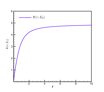
Setting , we have
which is strictly positive. This implies blows up for sufficiently small . For fixed , one can see from Figure 2 that is increasing with respect to . On the other hand, is also increasing with respect to , for fixed .
Example 1.4.
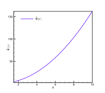
Assume that , , and . In this case, we denote and get
where is the third derivative of . Therefore, blows up as . Moreover, is increasing with respect to (see Figure 2).
The remainder of this paper is organized as follows. In section 2, we give the outline of the proof of Theorem 1.1 and reduce the proof of Theorem 1.1 to establishing the asymptotic formulae of , the singular function , and . In Section 3, we deal with the asymptotic formulae of , and by exploring several properties of the sequences and . In section 4 we are devoted to the proof of Proposition 2.3, which characterizes the asymptotic behavior of . The asymptotic formula of is given in Section 5.
2. Proof of Theorem 1.1
In this section, we are devoted to proving Theorem 1.1. We first introduce a singular function and establish its asymptotic formula by making use of our improvement on , and . Then we further investigate the asymptotic formula of , and obtain the blowup factor . We follow the notations in [35].
The main ingredient to prove Theorem 1.1 is the singular function , first introduced in [39], which is the solution to
| (2.1) |
The existence and uniqueness of the solution can be referred to [2, 39]. We emphasize that the constant values of on and on are different. So that becomes arbitrary large if goes to zero. Define the function by
| (2.2) |
Then one can see that is harmonic in and ; that is, there is no potential difference of on and . By using the same way as in [25, 30], we can show that is bounded on any bounded subset of . Thus, the function characterizes the singular behavior of the solution to (1.4), and the singular behavior of is determined by
Therefore, the proof of Theorem 1.1 is reduced to the estimates or expansions of , and .
To this end, we introduce the following notations. Let be the reflection with respect to , , i.e.,
Denote
| (2.3) |
and
| (2.4) |
where
| (2.5) |
Similarly,
and
where
| (2.6) |
Set
| (2.7) |
and
| (2.8) |
By using image charge method, Lim and Yun [35] obtained the following expression of , which has been used to derive estimates like (1.1).
Lemma 2.1.
The solution to (2.1) is given by
| (2.9) |
where is the fundamental solution of the Laplacian in three dimensions.
The following Proposition 2.2 gives the complete expressions of , , and the asymptotic formula of .
Proposition 2.2.
We remark that Lim and Yun in [35] obtained the upper and lower bounds of by using the estimates
| (2.10) |
Proposition 2.2 is an important improvement on , , which is the first difficulty that we overcome in this paper.
Let
be a narrow region in between and , where . Then we have the asymptotic formula of in .
Proposition 2.3.
For , we have
From (2.3)–(2.6) and Lemma 2.1, it is not difficult to see that
| (2.11) |
Finally, substituting these estimates above into the relationship [39, 40]
| (2.12) |
we have
Proposition 2.4.
Now, we are ready to prove Theorem 1.1.
Proof of Theorem 1.1..
Remark 2.5.
We now compare with the result in [26] for . When , the computation becomes easy to handle. In fact, by using the symmetry and (2.3)–(2.6), we have
In this case, we can rewrite
Hence,
and (2.9) becomes
which is the same as (1.22) in [26]. For general case , we should find the explicit expression of , and in terms of and .
3. Proof of Proposition 2.2
To prove Proposition 2.2, from the definitions of and , (2.7) and (2.8), we need to study some properties of the sequences and for , . Differently from the special case when in [26], where the symmetry of the domain makes the computation much easier to deal with, we now have to find the leading terms of , in terms of and .
3.1. Properties of the sequences and
In the following, we assume without loss of generality that . Set
We only consider the case when . If , then we replace and by and , respectively. We fix our notations now. For , we denote
Let be the fixed point of , then is the fixed point of . We emphasize that decreases to if is odd, and increases to if is even, . For readers’ convenience, we now list some results obtained in subsection 4.3 of [35] as follows.
| (3.1) |
and the sequence can be expressed as
| (3.2) |
| (3.3) |
where
| (3.4) |
and
| (3.5) |
For the sake of convenience, we will only deal with the case of for instance, since the argument for is the same. Recalling that and , then for simplicity, we use
| (3.6) |
to denote the main terms of and , , . We first choose an approximate number
which is fixed in [35] and is a constant independent of , and , so that the sequence terms of are dominant in the sequences and .
Lemma 3.1.
Let be defined as above. If , we have
| (3.7) |
and
| (3.8) |
where is independent of and .
The proof is very similar with that of Lemma 4.2 in [35]. We omit it here.
For a given , let and be as follows:
and
Here is the Gaussian bracket. Since is sufficiently small, we have
We have the following lemma.
Lemma 3.2.
-
(i)
There exists a positive constant C independent of and such that
(3.9) and
(3.10) - (ii)
-
(iii)
There exists a positive constant C independent of and such that for all , we have
(3.12) -
(iv)
and
Proof.
We first remark that the following and are independent of .
It follows from (3.2)–(3.5) that decreases to and increases to . Hence,
| (3.13) |
and
| (3.14) |
For , by using (2.4), (3.13), and (3.14), we have
| (3.15) |
Since is sufficiently small, it follows from (3.15), (3.8), and that
and
Remark 3.3.
Replacing by in (3.6), and recalling that and , we denote
Then, we have
and
Moreover, a direct calculation gives
| (3.17) |
| (3.18) |
Here, is independent of .
Now, we are ready to prove Proposition 2.2.
3.2. Proof of Proposition 2.2.
Proof of Proposition 2.2..
4. Proof of Proposition 2.3
4.1. The outline of the proof of Proposition 2.3
From the definition of , in order to prove Proposition 2.3, it suffices to establish the asymptotic formula of in . We first give the estimates of and , whose proof will be given in Subsection 4.2 later.
Lemma 4.1.
For , we have
for some constant C independent of and .
For the estimate of , especially the term for , is quite involved. In order to obtain the asymptotic formula of in the narrow region , we need to study the finer properties of the sequences and . The following Lemma is an adaption of Lemma 3.3 in [26]. Its proof is given in the Appendix.
Lemma 4.2.
-
(i)
If , then
(4.2) where is independent of and .
-
(ii)
There are positive constants and such that for all ,
(4.3)
Consider the following two auxiliary functions:
Define
Here, and are the fixed points of combined reflection and , respectively. We obtain the following two lemmas, whose proofs will be given in Subsection 4.3 and 4.4, respectively.
Lemma 4.3.
For , we have
and
Then
Lemma 4.4.
For , we have
Now, we are ready to prove Proposition 2.3.
4.2. Proof of Lemma 4.1
We first observe that if , then
Hence,
| (4.4) |
Using the notation
can be expressed as
where
Therefore, in order to estimate and , it suffices to estimate . We shall divide the rest of the proof into two steps.
Step 1. Estimates of and . Notice that
Therefore, we have
By (4.4), there exists some constant such that
It then follows that
For , we obtain from (3.8) that
| (4.5) |
It is easy see from Lemma 3.2 (iii) that
| (4.6) |
Then, by using (4.5) and (4.6), we have
| (4.7) |
Thus,
| (4.8) |
Similarly, is also bounded by the right-hand side of (4.8).
Step 2. Estimates of and . By a direct calculation, we have
| (4.9) |
Notice that
Recall (3.2) implies that
| (4.10) |
For , it results from (4.4) and (4.6) that
| (4.11) |
and
| (4.12) |
Hence, we have
Similar to (4.2), we have
| (4.13) |
A direct calculation gives
| (4.14) |
By the definition of , for , there is a constant C independent of and such that
By (2.3) and (3.7), we have for ,
| (4.15) |
Hence,
Similar to (4.2), is also bounded by the right-hand side of (4.13).
Notice that
For , using (3.7) and the fact that the sequence is decreasing to , we have
| (4.16) |
Then
| (4.17) |
On the other hand, recalling the fact that is increasing to , it follows from (4.4) and (3.1) that for all ,
| (4.18) |
Similarly,
| (4.19) |
It follows from (3.9), (4.17), and (4.18) that
For , by using (4.16), we have
| (4.20) |
Hence, we obtain from (3.9), (4.14), (4.18)–(4.2) that
Coming back to (4.2), we have
Similarly,
Lemma 4.1 is proved.
4.3. Proof of Lemma 4.3
By the definition of , we have
If , then for all , we have
for some constant . Since , we have . Thus, we have
| (4.21) |
Suppose now that . Using (4.4) and the fact that
again, we can see that for all , there exists some constant independent of and , such that
| (4.22) |
and
| (4.23) |
Thus, we have
| (4.24) |
4.4. Proof of Lemma 4.4
From the definitions of and , we have
and
The rest of the proof is divided into four steps.
Step 1. Estimates of , , , , and . By (4.4), one can see that for all , there is a constant independent of such that
So we have from (4.5) and (4.6) that
We use the fact that is decreasing to , is increasing to , and (ii) again to conclude that
Similarly, we have
By Lemma 3.2 (iv) and the definition of ,
Thus, we have showed that
We set
and
We claim that
| (4.27) |
| (4.28) |
and
| (4.29) |
Step 2. Proof of (4.27). We obtain from (3.7) that
This means that, for , we have
Hence, for , by using (2.3), we have
| (4.30) |
and
| (4.31) |
It follows from (4.4), (4.4), and Lemma 4.2 (i) that
(4.27) is thus proved.
By using (4.5), (4.10), and (4.11), we have
and
It follows from (3.9), (4.17), and (4.18) that
This means that
| (4.33) |
Notice that
We obtain from (4.15), (4.5), and (4.12) that if , then
| (4.34) |
If , then
| (4.35) |
Combining (3.9), (4.19), and (4.2), we deduce
| (4.36) |
By using (4.14) and the same argument that led to (4.4) and (4.36), we get and bounded by the right-hand side of (4.36). Thus,
| (4.37) |
Coming back to (4.4), we get (4.28) by using (4.33) and (4.37).
Step 4. Proof of (4.29). For , let
Define
By the mean value property, there is such that
Then, we have
First, recalling (4.4), one can show that there is some constant independent of , such that
We thus have
and
If , then we have
In view of (4.15), one can see that
Therefore, we have
By using the same argument that led to (4.34) and (4.4), we have
and
If , we have from (3.2) that
the last inequality holds since is sufficiently small and
A direct calculation gives that
By using Lemma 3.2 (ii), for all , we have
Since for all , we have
Thus, we have
| (4.38) |
Similarly, one can show that is also bounded by the right-hand side of (4.38). This completes the proof of (4.29).
5. Proof of Proposition 2.4
It has been proved in [39] and [40] that
| (5.1) |
Since is a constant on and , one can see from (5.1), (2.9), and Green’s representation formula that
| (5.2) |
Without loss of generality, we may assume that . Then for , by Lemma 3.1, we have
and
We thus have
where is independent of .
On the other hand, by Lemma 3.1, Lemma 3.2 (i) and , we have
and
Moreover,
and similarly,
Combining the above estimates, we obtain
By the similar way, we have
where
Therefore, coming back to (5) and recalling the definitions of and , (1) and (1), we obtain from Proposition 2.2 that
| (5.3) |
Remark 5.1.
When for some constant , combining (5.3) and (1.5), we can get
| (5.4) |
This is much more concise than the formula (57) in [28]. In fact, the author [28] proved that the average field which is the potential difference divided by the distance between two spheres with different radii, is given by
| (5.5) |
where is Euler-Mascheroni constant. For given , formulae (5.1) and (5.1) coincide up to for small enough .
6. Appendix
Proof of Lemma 4.2..
STEP 1. Proof of (i).
STEP 1.1. If , then it follows from (2.4), (3.13), and (3.14) that
By using the inequality , we obtain
| (6.1) |
where the error term satisfies
The last inequality above holds since is sufficiently small. We have from (6.1), (3.2), and (3.3) that
where
Since is decreasing in and is increasing in , we have
and
where
| (6.2) |
Thus, we have
where the new error term satisfies
| (6.3) |
One can see from (3.4) and (3.5) that
where
| (6.4) |
Then, we have
which in turn implies
| (6.5) |
where
| (6.6) |
Suppose now that , , then we have
We will show that
| (6.10) |
| (6.11) |
| (6.12) |
and
| (6.13) |
Once we have these estimates, then (i) results from (6). In the rest, we prove (6.10)–(6.13), one by one.
Step 1.2. Proofs of (6.10)–(6.13). To prove (6.10), we obtain from (3.1), (3.2), and (3.5) that
Similarly,
(6.10) is proved.
To prove (6.11), we first observe that
Since , , and , we have
It follows that
By the similar way,
(6.11) is proved.
To prove (6.12), we need to use the following inequality
| (6.14) |
Recalling that , , and
Taking in (6.14), we have
| (6.15) |
By using (3.8) with , we have
We thus have
here, we used
Similarly,
(6.12) is proved.
References
- [1] H. Ammari; E. Bonnetier; F. Triki; M. Vogelius, Elliptic estimates in composite media with smooth inclusions: an integral equation approach. Ann. Sci. c. Norm. Sup r. (4) 48 (2015), no. 2, 453-495.
- [2] H. Ammari; G. Ciraolo; H. Kang; H. Lee; K. Yun, Spectral analysis of the Neumann-Poincar operator and characterization of the stress concentration in anti-plane elasticity. Arch. Ration. Mech. Anal. 208 (2013), 275-304.
- [3] H. Ammari; H. Dassios; H. Kang; M. Lim, Estimates for the electric field in the presence of adjacent perfectly conducting spheres. Quat. Appl. Math. 65 (2007), 339-355.
- [4] H. Ammari; P. Garapon; H. Kang; H. Lee, A method of biological tissues elasticity reconstruction using magnetic resonance elastography measurements. Quart. Appl. Math. 66 (1) (2008), 139-175.
- [5] H. Ammari; H. Kang; H. Lee; J. Lee; M. Lim, Optimal estimates for the electric field in two dimensions. J. Math. Pures Appl. 88 (2007), 307-324.
- [6] H. Ammari; H. Kang; H. Lee; M. Lim; H. Zribi, Decomposition theorems and fine estimates for electrical fields in the presence of closely located circular inclusions. J. Differential Equations, 247 (2009), 2897-2912.
- [7] H. Ammari; H. Kang; M. Lim, Gradient estimates for solutions to the conductivity problem. Math. Ann. 332 (2005), 277-286.
- [8] I. Babuška; B. Andersson; P. Smith; K. Levin, Damage analysis of fiber composites. I. Statistical analysis on fiber scale. Comput. Methods Appl. Mech. Engrg. 172 (1999), 27-77.
- [9] E. Bao; Y.Y. Li; B. Yin, Gradient estimates for the perfect conductivity problem. Arch. Ration. Mech. Anal. 193 (2009), 195-226.
- [10] E. Bao; Y.Y. Li; B. Yin, Gradient estimates for the perfect and insulated conductivity problems with multiple inclusions. Comm. Partial Differential Equations, 35 (2010), 1982-2006.
- [11] J.G. Bao; H.J. Ju; H.G. Li, Optimal boundary gradient estimates for Lamé systems with partially infinite coefficients. Adv. Math. 314 (2017), 583-629.
- [12] J.G. Bao; H.G. Li; Y.Y. Li, Gradient estimates for solutions of the Lamé system with partially infinite coefficients. Arch. Ration. Mech. Anal. 215 (2015), no. 1, 307-351.
- [13] J.G. Bao; H.G. Li; Y.Y. Li, Gradient estimates for solutions of the Lamé system with partially infinite coefficients in dimensions greater than two. Adv. Math. 305 (2017), 298-338.
- [14] E. Bonnetier; F. Triki, Pointwise bounds on the gradient and the spectrum of the Neumann-Poincaré operator: the case of 2 discs, Multi-scale and high-contrast PDE: from modeling, to mathematical analysis, to inversion, 81-91, Contemp. Math., 577, Amer. Math. Soc., Providence, RI, 2012.
- [15] E. Bonnetier; F. Triki, On the spectrum of the Poincare variational problem for two close-to-touching inclusions in 2D. Arch. Ration. Mech. Anal. 209 (2013), 541-567.
- [16] E. Bonnetier; M. Vogelius, An elliptic regularity result for composite medium with ”Touching” fibers of circular cross-section. SIAM J. Math. Anal. 31 (2000), 651-677.
- [17] M. Briane; Y. Capdeboscq; L. Nguyen, Interior regularity estimates in high conductivity homogenization and application. Arch. Ration. Mech. Anal. 207 (1) (2013), 75-137.
- [18] B. Budiansky; G.F. Carrier, High shear stresses in stiff fiber composites. J. App. Mech. 51 (1984), 733-735.
- [19] H.J. Dong; H.G. Li, Optimal estimates for the conductivity problem by Green’s function method. arXiv: 1606.02793v1. (2016)
- [20] H.J. Dong; H. Zhang, On an elliptic equation arising from composite materials. Arch. Ration. Mech. Anal. 222 (2016), no. 1, 47-89.
- [21] Y. Gorb, Singular behavior of electric field of high-contrast concentrated composites. Multiscale Model. Simul. 13 (2015), no. 4, 1312-1326.
- [22] Y. Gorb; A. Novikov, Blow-up of solutions to a p-Laplace equation. Multiscale Model. Simul. 10 (2012), 727-743.
- [23] J.B. Keller, Conductivity of a medium containing a dense arrary of perfectly conducting spheres or cylinders or nonconducting cylinders. J. Appl. Phys. 34 (1963), 991-993.
- [24] J.B. Keller, Stresses in narrow regions. Trans. ASME J. Appl. Mech. 60 (1993), 1054-1056.
- [25] H. Kang; M. Lim; K. Yun, Asymptotics and computation of the solution to the conductivity equation in the presence of adjacent inclusions with extreme conductivities. J. Math. Pures Appl. 99 (2013), No. 9, 234-249.
- [26] H. Kang; M. Lim; K. Yun, Characterization of the electric field concentration between two adjacent spherical perfect conductors. SIAM J. Appl. Math. 74 (2014), 125-146.
- [27] H. Kang; K. Yun, Optimal estimates of the field enhancement in presence of a bow-tie structure of perfectly conducting inclusions in two dimensions. arXiv: 1707.00098v2. (2017).
- [28] J. Lekner, Near approach of two conducting spheres: Enhancement of external electric filed. J. Electrostatics. 69 (2011), 559-563.
- [29] H.G. Li; Y.Y. Li, Gradient estimates for parabolic systems from composite material. Science China Math. 60 (2017), No. 11, 2011-2052.
- [30] H.G. Li; Y.Y. Li; E.S. Bao; B. Yin, Derivative estimates of solutions of elliptic systems in narrow regions. Quart. Appl. Math. 72 (2014), no. 3, 589-596.
- [31] Y.Y. Li; L. Nirenberg, Estimates for elliptic system from composite material. Comm. Pure Appl. Math. 56 (2003), 892-925.
- [32] Y.Y. Li; M. Vogelius, Gradient estimates for solution to divergence form elliptic equation with discontinuous coefficients. Arch. Rational Mech. Anal. 153 (2000), 91-151.
- [33] H.G. Li and L.J. Xu, Optimal estimates for the perfect conductivity problem with inclusions close to the boundary. SIAM J. Math. Anal. 49 (2017), no. 4, 3125-3142.
- [34] M. Lim; S. Yu, Asymptotic analysis for superfocusing of the electric field in between two nearly touching metallic spheres. arXiv: 1412.2464v2. (2015).
- [35] M. Lim; K. Yun, Blow-up of electric fields between closely spaced spherical perfect conductors. Comm. Partial Differential Equations, 34 (2009), 1287-1315.
- [36] M. Lim; K. Yun, Strong influence of a small fiber on shear stress in fiber-reinforced composites. J. Differential Equations 250 (2011), 2402-2439.
- [37] A. Moradifam; A. Nachman; A. Tamasan, Conductivity imaging from one interior measurement in the presence of perfectly conducting and insulating inclusions. SIAM J. Math. Anal. 44 (2012), 3969-3990.
- [38] X. Markenscoff, Stress amplification in vanishingly small geometries. Comput. Mech. 19 (1996), 77-83.
- [39] K. Yun, Estimates for electric fields blown up between closely adjacent conductors with arbitrary shape. SIAM J. Appl. Math. 67 (2007), 714-730.
- [40] K. Yun, Optimal bound on high stresses occurring between stiff fibers with arbitrary shaped cross-sections. J. Math. Anal. Appl. 350 (2009), 306-312.
- [41] K. Yun, An optimal estimate for electric fields on the shortest line segment between two spherical insulators in three dimensions. J. Differential Equations, 261 (2016), No. 1, 148-188.
- [42] K. Yun, Two types of electric field enhancements by infinitely many circular conductors arranged closely in two parallel lines. Quart. Appl. Math. 75 (2017), 649-676.