Correlation functions for a spin-$\frac{1}{2}$ Ising-XYZ diamond chain: Further evidence for quasi-phases and pseudo-transitions

Abstract

One-dimensional systems with short-range interactions cannot exhibit a long-range order at nonzero temperature. However, there are some particular one-dimensional models, such as the Ising-Heisenberg spin models with a variety of lattice geometries, which exhibit unexpected behavior similar to the discontinuous or continuous temperature-driven phase transition. Although these pseudo-transitions are not true temperature-driven transitions showing only abrupt changes or sharp peaks in thermodynamic quantities, they may be confused while interpreting experimental data. Here we consider the spin-$\frac{1}{2}$ Ising-XYZ diamond chain in the regime when the model exhibits temperature-driven pseudo-transitions. We provide a detailed investigation of several correlation functions between distant spins that illustrates the properties of quasi-phases separated by pseudo-transitions. Inevitably, all correlation functions show the evidence of pseudo-transition, which are supported by the analytical solutions and, besides we provide a rigorous analytical investigation around the pseudo-critical temperature. It is worth to mention that the correlation functions between distant spins have an extremely large correlation length at pseudo-critical temperature.

1 Introduction

In the past decade, Cuesta and Sánchez [1] investigated relevant properties regarding one-dimensional models with short-range interaction, such as the general non-existence theorem for finite-temperature phase transitions [2]. Furthermore, there is a wide class of one-dimensional growth models subjected to an external field (i.e., with on-site periodic potential), such as the discrete sine-Gordon model, showing absence of phase transition at finite temperature. Despite the fact that for the one-dimensional discrete sine-Gordon model it has been proven that the model cannot have any phase transition at finite temperature [3], some numerical simulations strongly suggested the existence of apparent finite temperature separation between a flat region and rough phase. This result was investigated by Ares et al. [4] using the transfer operator formalism showing that an arbitrary size sine-Gordon chain will exhibit this apparent phase transition at finite temperature. Recently, it has been found that water molecules confined inside single-walled carbon nanotubes exhibit entirely different behavior from their bulk analogues: Such single-file chain of water molecules encapsulated in the tubes shows a temperature-driven quasi-phase transition [5]. On the other hand, using the formalism of micro-canonical ensemble it was also shown a pseudo-transition at finite temperature for a simple kinetic one-dimensional model [6].

Lately, several one-dimensional models have been examined in the framework of decorated structures, in particular, Ising and Heisenberg models with a variety of geometric structures, such as the Ising-Heisenberg models in diamond-chain structure [7, 8], the one-dimensional double-tetrahedral chain, in which the localized Ising spin regularly alternates with two mobile electrons delocalized over a triangular plaquette [9], the alternating Ising-Heisenberg ladder model [10], the Ising-Heisenberg triangular tube model [11]. These models show unexpected behavior similar to the discontinuous or continuous temperature-driven phase transition. The analysis of the first derivative of the free energy, such as entropy, internal energy, magnetization, shows an abrupt jump as a function of temperature, maintaining a close similarity with first-order phase transition. Whereas a second order derivative of free energy, such as specific heat and magnetic susceptibility, resembles a typical second-order phase transition at finite temperature. Although these pseudo-transitions are not the true temperature-driven transitions, abrupt changes or sharp peaks in thermodynamic quantities may lead to mistaken conclusions while interpreting experimental data.

Here our main goal is to shed further light on pseudo-transitions and to illustrate them discussing correlation functions around the pseudo-critical temperature. We take as an example the spin-$\frac{1}{2}$ Ising-XYZ diamond chain investigated in some details earlier [7, 8]. The rest of the paper is organized as follows. First, we review the model and its ground-state diagram considered in Refs. [7, 8, 12], Sec. 2. Then we discuss the pseudo-transitions from the effective Ising-chain-model perspective, Sec. 3. Our main findings are the distant pair spin correlation functions for the spin-$\frac{1}{2}$ Ising-XYZ diamond chain, which are examined rigorously in Sec. 4. Finally, we summarize our results in Sec. 5.

2 Hamiltonian of the model and its ground-state phases

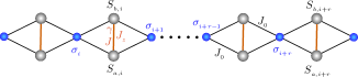
Figure 1: Schematic representation of spin-$\frac{1}{2}$ Ising-XYZ diamond chain.

Here we consider the Hamiltonian of the Ising-XYZ diamond chain, see Fig. 1, as the sum of the block Hamiltonians per unit cell $\mathcal{H}=\sum_{i=1}^{N}H_{i}$ already discussed in Ref. [7]. The Hamiltonian of the unit cell is given by:

$$H_{i}= - J(1+\gamma)S_{a,i}^{x}S_{b,i}^{x}-J(1-\gamma)S_{a,i}^{y}S_{b,i}^{y}-J_{z}S_{a,i}^{z}S_{b,i}^{z}$$ (1)

$$- J_{0}(S_{a,i}^{z}+S_{b,i}^{z})(\sigma_{i}+\sigma_{i+1})$$

$$- h_{z}(S_{a,i}^{z}+S_{b,i}^{z})-\frac{h}{2}(\sigma_{i}+\sigma_{i+1}),$$

where $S_{a(b)}^{\alpha}(\alpha=x,y,z)$ are the spin-$\frac{1}{2}$ operators, $\sigma$ corresponds to the Ising spins $\frac{1}{2}$, $\gamma$ is the $xy$-anisotropy parameter, $J$ and $J_{z}$ are the Heisenberg-like interactions between interstitial sites, the exchange parameter $J_{0}$ represents the Ising-like interaction between nodal and interstitial sites, and the external magnetic field $h_{z}$ and $h$ are assumed to be along the $z$-direction.

The eigenvalues of the Hamiltonian (1) for the $i$-th unit cell are given by:

$$\mathcal{E}_{1} = -h\frac{\mu}{2}-\frac{J_{z}}{4}+\Delta_{\mu},$$ (2)

$$\mathcal{E}_{2} = -h\frac{\mu}{2}-\frac{J}{2}+\frac{J_{z}}{4},$$ (3)

$$\mathcal{E}_{3} = -h\frac{\mu}{2}+\frac{J}{2}+\frac{J_{z}}{4},$$ (4)

$$\mathcal{E}_{4} = -h\frac{\mu}{2}-\frac{J_{z}}{4}-\Delta_{\mu},$$ (5)

where $\mu=\sigma_{i}+\sigma_{i+1}$ and $\Delta_{\mu}=\sqrt{(h_{z}+J_{0}\mu)^{2}+\frac{1}{4}J^{2}\gamma^{2}}$. The corresponding eigenstates in the natural basis $\{|\begin{smallmatrix}+\\ +\end{smallmatrix}\rangle,|\begin{smallmatrix}+\\ -\end{smallmatrix}\rangle,|\begin{smallmatrix}-\\ +\end{smallmatrix}\rangle,|\begin{smallmatrix}-\\ -\end{smallmatrix}\rangle\}$ are:

$$\left|\varphi_{1}\right> = -\sin\theta_{\mu}|\begin{smallmatrix}+\\ +\end{smallmatrix}\rangle+\cos\theta_{\mu}|\begin{smallmatrix}-\\ -\end{smallmatrix}\rangle,$$ (6)

$$\left|\varphi_{2}\right> = \frac{1}{\sqrt{2}}\left(|\begin{smallmatrix}-\\ +\end{smallmatrix}\rangle+|\begin{smallmatrix}+\\ -\end{smallmatrix}\rangle\right),$$ (7)

$$\left|\varphi_{3}\right> = \frac{1}{\sqrt{2}}\left(|\begin{smallmatrix}-\\ +\end{smallmatrix}\rangle-|\begin{smallmatrix}+\\ -\end{smallmatrix}\rangle\right),$$ (8)

$$\left|\varphi_{4}\right> = \cos\theta_{\mu}|\begin{smallmatrix}+\\ +\end{smallmatrix}\rangle+\sin\theta_{\mu}|\begin{smallmatrix}-\\ -\end{smallmatrix}\rangle,$$ (9)

where $\theta_{\mu}=\frac{1}{2}\tan^{-1}\frac{J\gamma}{2(h_{z}+J_{0}\mu)}$ with $0<\theta_{\mu}<\pi$.

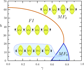
Figure 2: Ground-state phase diagram in the $\gamma-h$ plane. The coupling parameters are assumed as $J=100$, $J_{z}=24$, and $J_{0}=-24$.

Next, we provide a zero-temperature phase diagram in the $\gamma-h$ plane [7, 8, 12]. Throughout this article, we will consider only the case $h_{z}=h$. In Fig. 2 we report the ground-state phase diagram for a particular set of coupling parameters $J=100$, $J_{z}=24$, and $J_{0}=-24$. From now on we will consider just this set of parameters throughout the article. The phase diagram presents three ground-state phases, namely, one ferrimagnetic phase ($FI$) and two modulated ferromagnetic Heisenberg phases ($MF_{0}$ and $MF_{2}$). We use the term “modulated” since, e.g., the state $|\varphi_{4}\rangle$ has probability $\cos^{2}\theta_{\mu}$ in $|\begin{smallmatrix}+\\ +\end{smallmatrix}\rangle$ and $\sin^{2}\theta_{\mu}$ in $|\begin{smallmatrix}-\\ -\end{smallmatrix}\rangle$. Therefore, these states are given below:

$$\left|MF_{2}\right\rangle= \overset{N}{\underset{i=1}{\prod}}|\varphi_{4}\rangle_{i}\otimes|\uparrow\rangle_{i},$$ (10)

$$\left|FI\right\rangle= \overset{N}{\underset{i=1}{\prod}}|\varphi_{2}\rangle_{i}\otimes|\uparrow\rangle_{i},$$ (11)

$$\left|MF_{0}\right\rangle= \overset{N}{\underset{i=1}{\prod}}|\varphi_{4}\rangle_{i}\otimes|\downarrow\rangle_{i}.$$ (12)

The corresponding ground-state energies are:

$$\varepsilon_{1,0}=E_{{}_{MF_{2}}}= -\tfrac{J_{z}}{4}-\tfrac{h}{2}-\!\sqrt{(h_{z}\!+J_{0})^{2}+\tfrac{1}{4}J^{2}\gamma^{2}},$$ (13)

$$\varepsilon_{0,0}=E_{{}_{FI}}= \frac{J_{z}}{4}-\frac{J}{2}-\frac{h}{2},$$ (14)

$$\varepsilon_{-1,0}=E_{{}_{MF_{0}}}= -\tfrac{J_{z}}{4}+\tfrac{h}{2}-\!\sqrt{(h_{z}\!-J_{0})^{2}+\tfrac{1}{4}J^{2}\gamma^{2}};$$ (15)

the $\varepsilon$’s notations should not be confused with $\mathcal{E}$’s defined in Eqs. (2) – (5). Its worth to note that phases $MF_{2}$ and $MF_{0}$ are degenerate for a null magnetic field and $\gamma\gtrsim 0.5892$. For $\gamma\approx 0.5892..0.8314$, the external magnetic field splits the energy as $E_{{}_{MF_{2}}}>E_{{}_{MF_{0}}}$, whereas for $\gamma\gtrsim 0.8314$ the external magnetic field splits the energy as $E_{{}_{MF_{2}}}<E_{{}_{MF_{0}}}$. Further information about of these results can be found in Refs. [12, 8].

3 Effective constants $J_{{\rm{eff}}}$ and $h_{{\rm{eff}}}$ and pseudo-transitions

Using the decoration transformation [13, 14, 15, 16], we can map the spin-$\frac{1}{2}$ Ising-XYZ diamond chain onto the well-known spin-$\frac{1}{2}$ Ising chain, whose Hamiltonian is expressed by $\mathcal{H}_{{}_{{\rm eff}}}=\sum_{j=1}^{N}\tilde{H}_{j}$, where

$$\mathcal{\tilde{H}}_{j}=-E_{{}_{{\rm eff}}}^{0}-J_{{}_{\text{eff}}}\sigma_{j}\sigma_{j+1}-h_{{}_{\text{eff}}}\sigma_{j},$$ (16)

here $E_{{}_{{\rm eff}}}^{0}$, $J_{{}_{\text{eff}}}$, and $h_{{}_{\text{eff}}}$ are the parameters of the effective Hamiltonian. Through the decoration transformation [13, 14, 15, 16] these effective Ising-chain parameters can be obtained explicitly; thus we have

$$E_{{}_{\text{eff}}}^{0}= \frac{1}{4\beta}\ln\left(w_{1}w_{0}^{2}w_{-1}\right),$$ (17)

$$J_{{}_{\text{eff}}}= \frac{1}{\beta}\ln\left(\frac{w_{1}w_{-1}}{w_{0}^{2}}\right),$$ (18)

$$h_{{}_{\text{eff}}}= \frac{1}{\beta}\ln\left(\frac{w_{1}}{w_{-1}}\right),$$ (19)

where

$$w_{\mu}=2\,{\rm e}^{\frac{\beta\mu h}{2}}\left[{\rm e}^{-\frac{\beta J_{z}}{4}}{\rm ch}\tfrac{\beta J}{2}+{\rm e}^{\frac{\beta J_{z}}{4}}{\rm ch}\left(\beta\Delta_{\mu}\right)\right].$$ (20)

Here $\mu=\{-1,0,1\}$, $\beta=\frac{1}{k_{B}T}$, $T$ denotes the absolute temperature, and $k_{B}$ is the Boltzmann constant.

Along the boundary between $FI$ and $MF_{0}$ or between $FI$ and $MF_{2}$ the Boltzmann factors (20) satisfy the following relation $w_{1}\sim w_{-1}\geqslant w_{0}$, which implies that $w_{1}w_{-1}\geqslant w_{0}^{2}$. Therefore from Eq. (18) we conclude that $J_{{\rm eff}}\geqslant 0$ and the equality holds only at $T\rightarrow\infty$. Thus, for $T<\infty$, the effective parameter is positive $J_{{\rm eff}}>0$ (effective “ferromagnetic interaction”).

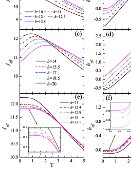
Figure 3: Effective Ising-chain parameters, assuming $J=100$, $J_{z}=24$, and $J_{0}=-24$. (a) Parameter $J_{{\rm{eff}}}$ as a function of temperature for $\gamma=0.7$. (b) Effective magnetic field $h_{{\rm{eff}}}$ as a function of temperature for $\gamma=0.7$. (c) $J_{{\rm{eff}}}$ against $T$ for $\gamma=0.75$. (d) $h_{{\rm{eff}}}$ against $T$ for $\gamma=0.75$. (e) $J_{{\rm{eff}}}$ against $T$ for $\gamma=0.8$. (f) $h_{{\rm{eff}}}$ against $T$ for $\gamma=0.8$.

In Fig. 3(a), (c), (e), the effective parameter $J_{{\rm eff}}$ (18) is depicted as a function of temperature for the above mentioned set of parameters, assuming several values for the magnetic field $h=h_{z}$. We observe that the effective parameter $J_{{\rm{eff}}}$ is always ferromagnetic and only weakly depends on temperature. In Fig. 3(b), (d), (f), the effective magnetic field $h_{{}_{\text{eff}}}$ (19) is illustrated. It is important to remark that the effective magnetic field $h_{{\rm{eff}}}$ may change its sign at a certain temperature, which will be discussed below.

Let us define the quasi-phases at a finite temperature as the zero-temperature phase extensions: $MF_{0}$ goes to $qMF_{0}$ and $FI$ goes to $qFI$. Thereby, in Fig. 3(f) one can see an interesting behavior of $h_{{\rm{eff}}}$ versus temperature $T$, namely, for $\gamma=0.8$ and $h=13$, the effective field $h_{{\rm{eff}}}$ remains almost zero until $T\approx 0.75$. But while $h_{{\rm eff}}<0$ the system is in $qMF_{0}$ phase, whereas for $h_{{\rm eff}}>0$ the system goes to $qMF_{2}$ phase, this will be confirmed when we study the magnetizations of Ising and Heisenberg spins (see Appendix B).

Hence, the necessary condition to find pseudo-transition is

$$h_{{\rm{eff}}}(T_{p})=0, {\rm and} w_{0}\ll\{w_{1},w_{-1}\}.$$ (21)

This equation is used to determine the temperature of the pseudo-transition. In Ref. [12], the equivalent condition, i.e., the requirement $w_{-1}=w_{1}$, was suggested. It leads to a transcendental equation for the pseudo-critical temperature $T_{p}$.

This phenomenon contrasts to the ordinary spin-$\frac{1}{2}$ ferromagnetic Ising chain in a field. The effective magnetic field orders all Ising spins but as the temperature increases the spins fluctuate and the ferromagnetic order immediately smoothly melts.

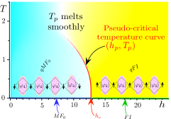
Figure 4: Phase diagram $T$ against $h$, obtained from the condition $h_{{\rm eff}}(T_{p})=0$, for fixed parameters $J=100$, $J_{z}=24$, $J_{0}=-24$, and $\gamma=0.7$.

In Fig. 4 the pseudo-critical temperature $T_{p}$, which is determined from the condition $h_{{\rm{eff}}}(T_{p})=0$, is shown (drawn as a solid red line). $T_{p}$ melts smoothly at $T_{p}\approx 1.5$. The phase diagram clearly shows the pseudo-critical temperature curve between two regions, the $qMF_{0}$ state and the $qFI$ state for the model in question with parameters given in Fig. 4. When $w_{0}$ becomes relevant, the condition $h_{{\rm{eff}}}(T_{p})=0$ still would give, in principle, the value of $T_{p}$, but this result does not lead to a pseudo-transition because the singularity observed when $w_{1}=w_{-1}$ vanishes due to the significant contribution of $w_{0}$. It is also worth mentioning that when $T_{p}\rightarrow 0$, then $h_{p}\rightarrow h_{c}$, where $h_{c}$ is the true critical magnetic field at the zero temperature.

Table 1: Pseudo-critical temperature for a given magnetic field with the parameters given in Fig. 4. First two columns correspond to $\gamma=0.7$, second two columns correspond to $\gamma=0.75$, and third two columns correspond to $\gamma=0.8$.

$\gamma=0.7$		$\gamma=0.75$		$\gamma=0.8$
$h$	$T_{p}$	$h$	$T_{p}$	$h$	$T_{p}$
$10$	$1.3552499$	$14$	$1.3552499$	$11$	$1.4753981$
$11$	$1.1270292$	$15.5$	$1.1270292$	$12.4$	$1.07033229$
$12$	$0.8150481$	$17$	$0.8150481$	$12.8$	$0.86683633$
$12.5$	$0.567641$	$18.5$	$0.567641$	$13$	$0.66742119$
$12.7$	$0.3726212$	$18.7$	$0.2671694$	$13.06$	$0.45524697$
$12.74$	$0.2694923$	$18.9$	$0.2057883$	$13.0639$	$0.2973970$
$\mathbf{12.75}$	$\mathbf{0.0}$	$\mathbf{19.22}$	$\mathbf{0.0}$	$\mathbf{13.063945}$	$\mathbf{0.0}$
$12.8$	No $T_{p}$	$20$	No $T_{p}$	$13.1$	No $T_{p}$

In Table 1 the pseudo-critical temperature is reported for several magnetic-field values using the condition (21). Here we assume the fixed $xy$-anisotropy parameters $\gamma=\{0.7,0.75,0.8\}$. For $\gamma=0.7$ this pseudo-critical temperature occurs in the interface between $qFI$ and $qMF_{0}$, whereas for $\gamma=0.75$ the pseudo-critical temperature occurs in the interface of $qFI$, $qMF_{0}$, and $qMF_{2}$. Analogously, for $\gamma=0.8$ the pseudo-critical temperature occurs in the boundary between $qMF_{0}$ and $qMF_{2}$. The next-to-last row of bold data corresponds to the critical field that occurs only at $T=0$, whereas the last row of data indicates that there is no pseudo-transition for $h>h_{c}$.

For the considered decorated chain, at some temperature (better low enough, then there still will be well pronounced traces of the ground-state ferromagnetic order) the effective magnetic field changes its sign. All Ising spins reorient simultaneously following the change in the effective field direction and continue to fluctuate with further temperature grow.

4 Spin correlations: Results and discussions

In this section, we study in detail the correlation functions for the model considered. To this end, we perform an algebraic procedure discussed in Ref. [17]. We write the transfer matrix as follows

$$\mathbf{W}=\left(\begin{array}[]{cc}w_{1}&w_{0}\\ w_{0}&w_{-1}\end{array}\right),$$ (22)

where $w_{1}$, $w_{0}$ and $w_{-1}$ are given by (20). Its eigenvalues are expressed by

$$\lambda_{\pm}=\frac{w_{1}+w_{-1}\pm B}{2}$$ (23)

with $B=\sqrt{\left(w_{1}-w_{-1}\right)^{2}+4w_{0}^{2}}$. The transfer matrix $\mathbf{W}$ in the diagonal basis becomes

$$\left(\begin{array}[]{cc}\lambda_{+}&0\\ 0&\lambda_{-}\end{array}\right)=\mathbf{P}^{-1}\mathbf{W}\,\mathbf{P}=\boldsymbol{\Lambda},$$ (24)

where the matrix $\mathbf{P}$ is written as

$$\mathbf{P}=\left(\begin{array}[]{cc}\cos\phi&-\sin\phi\\ \sin\phi&\cos\phi\end{array}\right)$$ (25)

with $\phi=\frac{1}{2}\tan^{-1}\frac{2w_{0}}{w_{1}-w_{-1}}$ and $0<\phi<\frac{\pi}{2}$. Therefore the partition function becomes $Z_{N}=\lambda_{+}^{N}+\lambda_{-}^{N}$ or for large $N$ simply becomes $Z_{N}=\lambda_{+}^{N}$.

Below there are two useful identities that will be used later. Namely,

$$\cos(2\phi)= \frac{w_{1}-w_{-1}}{B}=\frac{w_{1}-w_{-1}}{|w_{1}-w_{-1}|}\frac{1}{\sqrt{1+4\bar{w}_{0}^{2}}},$$

$$\sin(2\phi)= \frac{2w_{0}}{B}=\frac{2\bar{w}_{0}}{\sqrt{1+4\bar{w}_{0}^{2}}}>0,$$ (26)

where we define conveniently $\bar{w}_{0}=\frac{w_{0}}{\left|w_{1}-w_{-1}\right|}$.

The expectation value $\langle\sigma\rangle$ is expressed as follows

$$\langle\sigma\rangle=\frac{1}{\lambda_{+}^{N}}{\rm tr}\left(\sigma\mathbf{W}^{N}\right)=\frac{1}{\lambda_{+}^{N}}{\rm tr}\left(\tilde{\sigma}\boldsymbol{\Lambda}^{N}\right),$$ (27)

where $\tilde{\sigma}=\mathbf{P}^{-1}\sigma\mathbf{P}$ is explicitly given by

$$\tilde{\sigma}=\frac{1}{2}\left(\begin{array}[]{cc}\cos(2\phi)&-\sin(2\phi)\\ -\sin(2\phi)&-\cos(2\phi)\end{array}\right).$$ (28)

After some algebraic manipulations, we obtain

$$\langle\sigma\rangle=\frac{1}{2}\cos(2\phi)\left(1+u^{N}\right),$$ (29)

here $u=\tfrac{\lambda_{{}_{-}}}{\lambda_{{}_{+}}}$. In the thermodynamic limit, the formula for $\langle\sigma\rangle$ reduces to

$$\langle\sigma\rangle= \frac{1}{2}\cos(2\phi)=\frac{1}{2}\frac{w_{1}-w_{-1}}{|w_{1}-w_{-1}|}\frac{1}{\sqrt{1+4\bar{w}_{0}^{2}}}.$$ (30)

The Ising spin magnetization $M_{I}=\langle\sigma\rangle$ close to the pseudo-transition temperature becomes approximately

$$M_{I}=\frac{1}{2}\frac{w_{1}-w_{-1}}{|w_{1}-w_{-1}|}\left[1-2\bar{w}_{0}^{2}+\mathcal{O}(\bar{w}_{0}^{4})\right].$$ (31)

Consequently, the magnetization near the pseudo-transition can be expressed explicitly as

$$M_{I}=\begin{cases}\frac{1}{2}-\bar{w}_{0}^{2}+\mathcal{O}(\bar{w}_{0}^{4}),&w_{1}>w_{-1},\\ -\frac{1}{2}+\bar{w}_{0}^{2}+\mathcal{O}(\bar{w}_{0}^{4}),&w_{1}<w_{-1}.\end{cases}$$ (32)

Next we will study the correlation functions. Consider first the thermal average of two different Ising spins

$$\langle\sigma_{j}\sigma_{j+r}\rangle= \frac{1}{\lambda_{+}^{N}}{\rm tr}\left(\sigma\mathbf{W}^{r}\sigma\mathbf{W}^{N-r}\right)=\frac{1}{\lambda_{+}^{N}}{\rm tr}\left(\tilde{\sigma}\boldsymbol{\Lambda}^{r}\tilde{\sigma}\boldsymbol{\Lambda}^{N-r}\right)$$ (33)

with $r=\{0,1,2,\dots\}$. In fact, we are interested in the thermodynamic limit ($N\rightarrow\infty$) and this equation reduces to

$$\langle\sigma_{j}\sigma_{j+r}\rangle =\frac{1}{4}\left[\cos^{2}(2\phi)+u^{r}\sin^{2}(2\phi)\right]$$

$$=\langle\sigma\rangle^{2}+\frac{1}{4}u^{r}\sin^{2}(2\phi)=\langle\sigma\rangle^{2}+\left(\tfrac{w_{0}}{B}\right)^{2}u^{r}.$$ (34)

The case $r=0$ corresponds to the trivial identity $\langle\sigma^{2}\rangle=\frac{1}{4}$. Now let us discuss the average spin pair (34) around the pseudo-transition temperature when $\bar{w}_{0}\rightarrow 0$. We have

$$\langle\sigma_{j}\sigma_{j+r}\rangle=\begin{cases}\langle\sigma\rangle^{2}+\bar{w}_{0}^{2}\left(\tfrac{w_{-1}}{w_{1}}\right)^{r}+\mathcal{O}\left(\bar{w}_{0}^{4}\right),&w_{1}>w_{-1},\\ \langle\sigma\rangle^{2}+\bar{w}_{0}^{2}\left(\tfrac{w_{1}}{w_{-1}}\right)^{r}+\mathcal{O}\left(\bar{w}_{0}^{4}\right),&w_{1}<w_{-1}.\end{cases}$$ (35)

Therefore, after using (34), the correlation function $C_{I}=\langle\sigma_{j}\sigma_{j+r}\rangle-\langle\sigma\rangle^{2}$ becomes

$$C_{I}=\left(\tfrac{w_{0}}{B}\right)^{2}u^{r},$$ (36)

and close to the pseudo-transition ($\bar{w}_{0}\rightarrow 0$) the correlation function reduces to

$$C_{I}=\begin{cases}\bar{w}_{0}^{2}\left(\tfrac{w_{-1}}{w_{1}}\right)^{r}+\mathcal{O}\left(\bar{w}_{0}^{4}\right),&w_{1}>w_{-1},\\ \bar{w}_{0}^{2}\left(\tfrac{w_{1}}{w_{-1}}\right)^{r}+\mathcal{O}\left(\bar{w}_{0}^{4}\right),&w_{1}<w_{-1}.\end{cases}$$ (37)

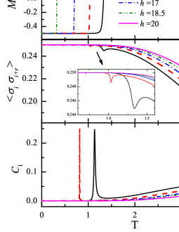
Figure 5: (a) Ising spin magnetization as a function of temperature. (b) Thermal average $\langle\sigma_{i}\sigma_{i+r}\rangle$, $r=1$ as a function of temperature. (c) Correlation function with $r=1$ as a function of temperature. We assume $J=100$, $J_{z}=24$, $J_{0}=-24$, and $\gamma=0.75$.

In Fig. 5(a) we show the temperature dependence of the Ising spin magnetization. For $w_{1}<w_{-1}$ the magnetization at $T=0$ is $M_{I}=-\frac{1}{2}$. Similarly, for $w_{1}>w_{-1}$, the magnetization in the limit of low temperature tends to $M_{I}\rightarrow\frac{1}{2}$, but holding the condition $w_{1}>w_{-1}$. This change occurs at $h_{{\rm eff}}(T_{p})=0$. For higher temperatures, the Ising spin magnetization decreases with temperature, as is expected in ordinary spin models.

In Fig. 5(b) the average $\langle\sigma_{j}\sigma_{j+r}\rangle$ is illustrated as a function of temperature. For $T\sim T_{p}$, we have $\langle\sigma_{j}\sigma_{j+r}\rangle\rightarrow\frac{1}{4}$ for both cases $w_{1}>w_{-1}$ or $w_{1}<w_{-1}$. In principle, it looks as a monotonically decreasing curve, but as soon as the magnetic field becomes closer to $h\rightarrow h_{c}$, it exhibits a non-monotonic temperature behavior suppressed at $T_{p}$ according to Eq. (35).

In Fig. 5(c) the correlation function (36) is plotted against the temperature. Here, we can observe a peak at the pseudo-critical temperature, the lower the temperature is, the thinner and higher the peak is, whereas the higher the temperature is, the broader the peak is.

To estimate the magnetization of the Heisenberg spin, we must apply the decoration transformation approach [13, 14, 15, 16]. First, we have to perform a partial trace over the Heisenberg spins. For this we need the unit cell Hamiltonian (1) with eigenvalues given by Eqs. (2) – (5) and the corresponding eigenvectors given by Eqs. (6) – (9). With the eigenstates in hand, we can construct a matrix $\mathbf{Q}$ as follows

$$\mathbf{Q}=\left(\begin{array}[]{cccc}-\sin\theta_{\mu}&0&0&\cos\theta_{\mu}\\ 0&\frac{1}{\sqrt{2}}&-\frac{1}{\sqrt{2}}&0\\ 0&\frac{1}{\sqrt{2}}&\frac{1}{\sqrt{2}}&0\\ \cos\theta_{\mu}&0&0&\sin\theta_{\mu}\end{array}\right),$$ (38)

remembering that $\theta_{\mu}$ was already specified when the eigenstates (6) – (9) were defined. The matrix $\mathbf{Q}$ diagonalizes the operator $H_{i}$, so any function of the operator $H_{i}$ will also be diagonalized, hence we have

$$\mathbf{D}=\mathbf{Q}^{-1}{\rm e}^{-\beta H_{i}(\sigma,\sigma^{\prime})}\mathbf{Q}.$$ (39)

Consequently, the matrix representation of the operator ${\rm e}^{-\beta H_{i}(\sigma,\sigma^{\prime})}$ can be written in terms of the eigenstates (2) – (5),

$$\mathbf{D}=\left(\begin{array}[]{cccc}{\rm e}^{-\beta\mathcal{E}_{1}}&0&0&0\\ 0&{\rm e}^{-\beta\mathcal{E}_{2}}&0&0\\ 0&0&{\rm e}^{-\beta\mathcal{E}_{3}}&0\\ 0&0&0&{\rm e}^{-\beta\mathcal{E}_{4}}\end{array}\right).$$ (40)

The Heisenberg spin operators $S_{a}^{\alpha}$ and $S_{b}^{\alpha}$ can be expressed as $\mathbf{s}_{a}^{\alpha}=S_{a}^{\alpha}\otimes\boldsymbol{1}_{b}$ and $\mathbf{s}_{b}^{\alpha}=\boldsymbol{1}_{a}\otimes S_{b}^{\alpha}$, respectively, and using the similarity transformation we have $\hat{\mathbf{s}}_{a}^{\alpha}=\mathbf{Q}^{-1}\mathbf{s}_{a}^{\alpha}\mathbf{Q}$ and $\hat{\mathbf{s}}_{b}^{\alpha}=\mathbf{Q}^{-1}\mathbf{s}_{b}^{\alpha}\mathbf{Q}$. The explicit representation of these matrices is given in Appendix A.

In what follows, we perform the partial trace over the Heisenberg spin operators,

$$w_{\mu}^{z}= {\rm tr}\left(\hat{\mathbf{s}}_{a}^{z}\mathbf{D}\right)={\rm tr}\left(\hat{\mathbf{s}}_{b}^{z}\mathbf{D}\right)$$

$$= {\rm e}^{\beta\left(\frac{h\mu}{2}+\frac{J_{z}}{4}\right)}\cos(2\theta_{\mu})\sinh(\beta\Delta_{\mu})=\frac{h_{z}+\mu J_{0}}{\Delta_{\mu}}{\rm e}^{\beta\left(\frac{h\mu}{2}+\frac{J_{z}}{4}\right)}\sinh(\beta\Delta_{\mu}).$$ (41)

The reason why we use the notation $w_{\mu}^{z}$ is because there is a relation with $w_{\mu}$:

$$w_{\mu}^{z}=\frac{1}{2\beta}\frac{\partial w_{\mu}}{\partial h_{z}}.$$ (42)

Evidently, using (42) we can recover the previous result (41). Now we define the matrix $\mathbf{W}_{z}$ as follows

$$\mathbf{W}_{z}=\left(\begin{array}[]{cc}w_{1}^{z}&w_{0}^{z}\\ w_{0}^{z}&w_{-1}^{z}\end{array}\right),$$ (43)

its elements are given by (41).

We are ready now to deal with the expectation values $\langle S_{a}^{z}\rangle$ and $\langle S_{b}^{z}\rangle$ (of course, $\langle S_{a}^{z}\rangle$ and $\langle S_{b}^{z}\rangle$ are identical). Thus, we have

$$\langle S_{a}^{z}\rangle=\langle S_{b}^{z}\rangle=\langle S^{z}\rangle=\frac{1}{\lambda_{+}^{N}}{\rm tr}\left(\mathbf{W}_{z}\;\mathbf{W}^{N-1}\right).$$ (44)

Using the similarity transformation given by $\mathbf{\widetilde{W}}_{z}=\mathbf{P}^{-1}\mathbf{W}_{z}\mathbf{P}$, we can write

$$\mathbf{\widetilde{W}}_{z}=\left(\begin{array}[]{cc}\tilde{w}_{1}^{z}&\tilde{w}_{0}^{z}\\ \tilde{w}_{0}^{z}&\tilde{w}_{-1}^{z}\end{array}\right).$$ (45)

Its elements are specified by

$$\tilde{w}_{1}^{z}= w_{1}^{z}\cos^{2}\phi+w_{-1}^{z}\sin^{2}\phi+w_{0}^{z}\sin(2\phi),$$ (46)

$$\tilde{w}_{0}^{z}= w_{0}^{z}\cos(2\phi)-\frac{1}{2}(w_{1}^{z}-w_{-1}^{z})\sin(2\phi),$$ (47)

$$\tilde{w}_{-1}^{z}= w_{1}^{z}\sin^{2}\phi+w_{-1}^{z}\cos^{2}\phi-w_{0}^{z}\sin(2\phi).$$ (48)

Eliminating the trigonometric functions using Eqs. (93) and (94), we can also write

$$\tilde{w}_{1}^{z}= \tfrac{\left(w_{1}^{z}+w_{-1}^{z}\right)}{2}+\tfrac{\left(w_{1}^{z}-w_{-1}^{z}\right)\left(w_{1}-w_{-1}\right)}{2B}+\tfrac{2w_{0}^{z}w_{0}}{B},$$ (49)

$$\tilde{w}_{0}^{z}= \tfrac{w_{0}^{z}\left(w_{1}-w_{-1}\right)}{B}-\tfrac{w_{0}\left(w_{1}^{z}-w_{-1}^{z}\right)}{B},$$ (50)

$$\tilde{w}_{-1}^{z}= \tfrac{\left(w_{1}^{z}+w_{-1}^{z}\right)}{2}-\tfrac{\left(w_{1}^{z}-w_{-1}^{z}\right)\left(w_{1}-w_{-1}\right)}{2B}-\tfrac{2w_{0}^{z}w_{0}}{B}.$$ (51)

Finally, the thermal average of the Heisenberg spin becomes,

$$\langle S^{z}\rangle= \frac{1}{\lambda_{+}^{N}}{\rm tr}\left(\mathbf{\widetilde{W}}_{z}\;\boldsymbol{\Lambda}^{N-1}\right)$$

$$= \frac{1}{\lambda_{+}^{N}}\left(\tilde{w}_{1}^{z}\lambda_{+}^{N-1}+\tilde{w}_{-1}^{z}\lambda_{-}^{N-1}\right).$$ (52)

We are interested in the thermodynamic limit, so the relation (52) results in

$$\langle S^{z}\rangle= \frac{\tilde{w}_{1}^{z}}{\lambda_{+}}$$

$$= \tfrac{\left(w_{1}^{z}+w_{-1}^{z}\right)}{2\lambda_{+}}+\tfrac{\left(w_{1}^{z}-w_{-1}^{z}\right)\left(w_{1}-w_{-1}\right)}{2B\lambda_{+}}+\tfrac{2w_{0}^{z}w_{0}}{B\lambda_{+}}.$$ (53)

It is worth expressing the average $\langle S^{z}\rangle$ around the pseudo-critical temperature since this analysis is our main goal. After performing some algebraic computations, we obtain:

$$\langle S^{z}\rangle=\frac{\tilde{w}_{1}^{z}}{\lambda_{+}}= \frac{h_{z}+J_{0}}{\Delta_{1}w_{1}}{\rm e}^{\beta\left(\frac{h}{2}+\frac{J_{z}}{4}\right)}\sinh(\beta\Delta_{1})$$

$$+\frac{2h_{z}}{\Delta_{0}w_{1}}{\rm e}^{\frac{\beta J_{z}}{4}}\sinh(\beta\Delta_{0})\,\bar{w}_{0}+\mathcal{O}\left(\bar{w}_{0}^{2}\right)$$ (54)

for $w_{1}>w_{-1}$ and

$$\langle S^{z}\rangle=\frac{\tilde{w}_{1}^{z}}{\lambda_{+}}= \frac{h_{z}-J_{0}}{\Delta_{-1}w_{-1}}{\rm e}^{\beta\left(-\frac{h}{2}+\frac{J_{z}}{4}\right)}\sinh(\beta\Delta_{-1})$$

$$+\frac{2h_{z}}{\Delta_{0}w_{-1}}{\rm e}^{\frac{\beta J_{z}}{4}}\sinh(\beta\Delta_{0})\,\bar{w}_{0}+\mathcal{O}\left(\bar{w}_{0}^{2}\right)$$ (55)

for $w_{-1}>w_{1}$. The Heisenberg spin magnetization is obtained from $M_{H}=\langle S^{z}\rangle$. In an analogous way, we can verify that the magnetizations of Heisenberg spin along the $x$ and $y$-axes are zero,

$$\langle S_{a}^{x}\rangle=\langle S_{a}^{y}\rangle=\langle S_{b}^{x}\rangle=\langle S_{b}^{y}\rangle=0.$$ (56)

Before we pass to computation of the correlation functions between neighboring cells, we study at first the two distant Heisenberg spins average, which can be obtained from

$$\langle S_{j}^{z}S_{j+r}^{z}\rangle=\frac{1}{\lambda_{+}^{N}}{\rm tr}\left(\mathbf{\widetilde{W}}_{z}\;\boldsymbol{\Lambda}^{r-1}\mathbf{\widetilde{W}}_{z}\;\boldsymbol{\Lambda}^{N-r-1}\right),$$ (57)

here $r=\{1,2,3,\dots\}.$ After some algebraic manipulations and bearing in mind the thermodynamic limit, we obtain

$$\langle S_{j}^{z}S_{j+r}^{z}\rangle= \frac{\left(\tilde{w}_{1}^{z}\right)^{2}}{\lambda_{+}^{2}}+\frac{\left(\tilde{w}_{0}^{z}\right)^{2}}{\lambda_{+}\lambda_{-}}u^{r}=\langle S^{z}\rangle^{2}+\frac{\left(\tilde{w}_{0}^{z}\right)^{2}}{\lambda_{+}\lambda_{-}}u^{r}.$$ (58)

Close to the pseudo-critical temperature ($\bar{w}_{0}\rightarrow 0$), the average $\langle S_{j}^{z}S_{j+r}^{z}\rangle$ up to first order in $\bar{w}$ becomes:

$$\langle S_{j}^{z}S_{j+r}^{z}\rangle= \langle S^{z}\rangle^{2}\!+\!\frac{\left(w_{0}^{z}\right)^{2}}{w_{1}w_{-1}}\negmedspace\left(\!1\!+\!2\frac{w_{-1}^{z}-w_{1}^{z}}{w_{0}^{z}}\bar{w}_{0}\!\right)\negmedspace\left(\frac{w_{-1}}{w_{1}}\right)^{r}$$

$$= \left(\frac{w_{1}^{z}}{w_{1}}\right)^{2}\left(1+4\frac{w_{0}^{z}}{w_{1}^{z}}\bar{w}_{0}\right)+\frac{\left(w_{0}^{z}\right)^{2}}{w_{1}w_{-1}}\left(1+2\frac{w_{-1}^{z}-w_{1}^{z}}{w_{0}^{z}}\bar{w}_{0}\right)\left(\frac{w_{-1}}{w_{1}}\right)^{r}$$

$$= \left(\frac{w_{1}^{z}}{w_{1}}\right)^{2}+\frac{\left(w_{0}^{z}\right)^{2}}{w_{1}w_{-1}}\left(\frac{w_{-1}}{w_{1}}\right)^{r}$$

$$+\!\frac{2w_{0}^{z}}{w_{1}}\negmedspace\left[\frac{2w_{1}^{z}}{w_{1}}\!+\!\frac{w_{-1}^{z}-w_{1}^{z}}{w_{-1}}\negmedspace\left(\frac{w_{-1}}{w_{1}}\right)^{r}\right]\bar{w}_{0}$$ (59)

for $w_{1}>w_{-1}$ and

$$\langle S_{j}^{z}S_{j+r}^{z}\rangle= \left(\frac{w_{-1}^{z}}{w_{-1}}\right)^{2}+\frac{\left(w_{0}^{z}\right)^{2}}{w_{1}w_{-1}}\left(\frac{w_{1}}{w-_{1}}\right)^{r}$$

$$+\!\frac{2w_{0}^{z}}{w_{-1}}\negmedspace\left[\!\frac{2w_{-1}^{z}}{w_{-1}}\!+\!\frac{w_{1}^{z}\!-\!w_{-1}^{z}}{w_{1}}\negmedspace\left(\negmedspace\frac{w_{1}}{w-_{1}}\negmedspace\right)^{\negmedspace r}\right]\!\bar{w}_{0}$$ (60)

for $w_{-1}>w_{1}$. From (58) the correlation function $C_{H}=\langle S_{j}^{z}S_{j+r}^{z}\rangle-\langle S^{z}\rangle^{2}$ becomes

$$C_{H}=\frac{\left(\tilde{w}_{0}^{z}\right)^{2}}{\lambda_{+}\lambda_{-}}u^{r}.$$ (61)

Near the pseudo-critical temperature, the correlation function is expressed by

$$C_{H}=\begin{cases}\frac{\left(w_{0}^{z}\right)^{2}}{w_{1}w_{-1}}\negmedspace\left(\!1\!+\!2\frac{w_{-1}^{z}-w_{1}^{z}}{w_{0}^{z}}\bar{w}_{0}\!\right)\negmedspace\left(\frac{w_{-1}}{w_{1}}\right)^{r},&w_{1}>w_{-1},\\ \frac{\left(w_{0}^{z}\right)^{2}}{w_{1}w_{-1}}\negmedspace\left(\!1\!-\!2\frac{w_{-1}^{z}-w_{1}^{z}}{w_{0}^{z}}\bar{w}_{0}\!\right)\negmedspace\left(\frac{w_{1}}{w-_{1}}\right)^{r},&w_{1}<w_{-1}.\end{cases}$$ (62)

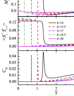
Figure 6: (a) Magnetization per unit cell as a function of temperature. (b) Average $\langle S_{j}^{z}S_{j+r}^{z}\rangle$, $r=1$ as a function of temperature. (c) Heisenberg spin correlation function with $r=1$ as a function of temperature. All plots are presented for the fixed set of parameters $J=100$, $J_{z}=24$, $J_{0}=-24$, and $\gamma=0.75$.

In Fig. 6(a) we show the temperature dependence of the Heisenberg spin magnetization for fixed parameters given in the caption to Fig. 6 for the range of $h$ values considered in Fig. 2. The behavior of the Heisenberg spin magnetization versus temperature is in agreement with Eq. (53), and in the limiting cases close to the pseudo-transition is given by Eqs. (54) and (55). Obviously, at $T=0$ the magnetization is in agreement with the ground-state phase diagram [the zeroth order of Eqs. (54) and (55)].

In Fig. 6(b) the pair Heisenberg spin average $\langle S_{i}^{z}S_{i+r}^{z}\rangle$ is displayed for the same set of parameters. Only the $z$-components of Heisenberg spins correlate. Below $T_{p}$ the Heisenberg spins are ordered and $\langle S_{i}^{z}S_{i+r}^{z}\rangle\rightarrow M_{H}^{2}$. However, for the temperature above $T_{p}$ or at relatively higher temperatures the correlation functions decreases gradually when $T\to\infty$ as expected for any standard spin chain.

Now we address our investigation to present the quantities which refer to one cell. So we perform the partial trace over the Heisenberg-Heisenberg spins operators,

$$v_{\mu}^{x}= {\rm tr}\left(\hat{\mathbf{s}}_{a}^{x}\hat{\mathbf{s}}_{b}^{x}\mathbf{D}\right)=\tfrac{1}{2}{\rm e}^{\frac{\beta\mu h}{2}}\negthickspace\left[{\rm e}^{-\frac{\beta J_{z}}{4}}{\rm sh}\negthickspace\tfrac{\beta J}{2}\!-{\rm e}^{\frac{\beta J_{z}}{4}}{\rm sh}\negthickspace\left(\beta\Delta_{\mu}\!\right)\!\cos(2\theta_{\mu})\right]\negthickspace,$$ (63)

$$v_{\mu}^{y}= {\rm tr}\left(\hat{\mathbf{s}}_{a}^{y}\hat{\mathbf{s}}_{b}^{y}\mathbf{D}\right)=\tfrac{1}{2}{\rm e}^{\frac{\beta\mu h}{2}}\negthickspace\left[{\rm e}^{-\frac{\beta J_{z}}{4}}{\rm sh}\negthickspace\tfrac{\beta J}{2}\!+{\rm e}^{\frac{\beta J_{z}}{4}}{\rm sh}\negthickspace\left(\beta\Delta_{\mu}\!\right)\!\cos(2\theta_{\mu})\right]\negthickspace,$$ (64)

$$v_{\mu}^{z}= {\rm tr}\left(\hat{\mathbf{s}}_{a}^{z}\hat{\mathbf{s}}_{b}^{z}\mathbf{D}\right)=\tfrac{1}{2}{\rm e}^{\frac{\beta\mu h}{2}}\left[{\rm e}^{\frac{\beta J_{z}}{4}}{\rm ch}\left(\beta\Delta_{\mu}\right)-{\rm e}^{-\frac{\beta J_{z}}{4}}{\rm ch}\left(\tfrac{\beta J}{2}\right)\right].$$ (65)

Therefore, the corresponding matrix can be written as

$$\mathbf{V}_{\alpha}=\left(\begin{array}[]{cc}v_{1}^{\alpha}&v_{0}^{\alpha}\\ v_{0}^{\alpha}&v_{-1}^{\alpha}\end{array}\right),$$ (66)

with $\alpha=\{x,y,z\}$. Using the similarity transformation given by $\mathbf{\widetilde{V}}_{\alpha}=\mathbf{P}^{-1}\mathbf{V}_{\alpha}\mathbf{P}$, we have

$$\mathbf{\tilde{V}}_{\alpha}=\left(\begin{array}[]{cc}\tilde{v}_{1}^{\alpha}&\tilde{v}_{0}^{\alpha}\\ \tilde{v}_{0}^{\alpha}&\tilde{v}_{-1}^{\alpha}\end{array}\right),$$ (67)

with the matrix elements

$$\tilde{v}_{1}^{\alpha}= v_{1}^{\alpha}\cos^{2}\phi+v_{-1}^{\alpha}\sin^{2}\phi+v_{0}^{\alpha}\sin(2\phi),$$ (68)

$$\tilde{v}_{0}^{\alpha}= v_{0}^{\alpha}\cos(2\phi)-\frac{1}{2}(v_{1}^{\alpha}-v_{-1}^{\alpha})\sin(2\phi),$$ (69)

$$\tilde{v}_{-1}^{\alpha}= v_{1}^{\alpha}\sin^{2}\phi+v_{-1}^{\alpha}\cos^{2}\phi-v_{0}^{\alpha}\sin(2\phi).$$ (70)

By eliminating the trigonometric functions, the elements of matrix $\mathbf{\tilde{V}}_{\alpha}$ become

$$\tilde{u}_{1}^{\alpha}= \tfrac{\left(u_{1}^{\alpha}+u_{-1}^{\alpha}\right)}{2}+\tfrac{\left(u_{1}^{\alpha}-u_{-1}^{\alpha}\right)\left(w_{1}-w_{-1}\right)}{2B}+\tfrac{2u_{0}^{\alpha}w_{0}}{B},$$ (71)

$$\tilde{u}_{0}^{\alpha}= \tfrac{u_{0}^{\alpha}\left(w_{1}-w_{-1}\right)}{B}-\tfrac{w_{0}\left(u_{1}^{\alpha}-u_{-1}^{\alpha}\right)}{B},$$ (72)

$$\tilde{u}_{-1}^{\alpha}= \tfrac{\left(u_{1}^{\alpha}+u_{-1}^{\alpha}\right)}{2}-\tfrac{\left(u_{1}^{\alpha}-u_{-1}^{\alpha}\right)\left(w_{1}-w_{-1}\right)}{2B}-\tfrac{2u_{0}^{\alpha}w_{0}}{B}.$$ (73)

Consequently, the average of the one-cell pair of Heisenberg spins is given by

$$\langle S_{a,j}^{\alpha}S_{b,j}^{\alpha}\rangle= \frac{1}{\lambda_{+}^{N}}{\rm tr}\left(\mathbf{\widetilde{V}}_{\alpha}\;\boldsymbol{\Lambda}^{N-1}\right)=\frac{1}{\lambda_{+}^{N}}\left(\tilde{v}_{1}^{\alpha}\lambda_{+}^{N-1}+\tilde{v}_{-1}^{\alpha}\lambda_{-}^{N-1}\right).$$ (74)

In the thermodynamic limit, we have

$$\langle S_{a,j}^{\alpha}S_{b,j}^{\alpha}\rangle\!= \tfrac{\left(v_{1}^{\alpha}+v_{-1}^{\alpha}\right)}{2\lambda_{+}}+\tfrac{\left(v_{1}^{\alpha}-v_{-1}^{\alpha}\right)\left(w_{1}-w_{-1}\right)}{2B\lambda_{+}}+\tfrac{2v_{0}^{\alpha}w_{0}}{B\lambda_{+}}.$$ (75)

In addition, the averages $\langle S_{a}^{x}S_{b}^{x}\rangle$, $\langle S_{a}^{y}S_{b}^{y}\rangle$, and $\langle S_{a}^{z}S_{b}^{z}\rangle$ satisfy the following identity

$$\langle S_{a}^{x}S_{b}^{x}\rangle+\langle S_{a}^{y}S_{b}^{y}\rangle+\langle S_{a}^{z}S_{b}^{z}\rangle=\frac{1}{4}$$ (76)

at any temperature. This is a simple consequence of the obvious relation $\langle({\bf{S}}_{a}+{\bf{S}}_{b})^{2}\rangle=S(S+1)=2$.

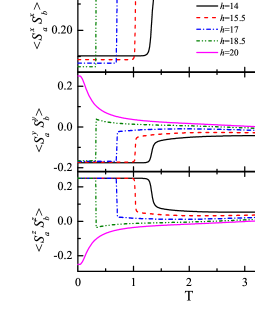
Figure 7: One-cell pair average ($r=0$) as a function of temperature. (a) $\langle S_{a}^{x}S_{b}^{x}\rangle$; (b) $\langle S_{a}^{y}S_{b}^{y}\rangle$; (c) $\langle S_{a}^{z}S_{b}^{z}\rangle$. We assume $J=100$, $J_{z}=24$, $J_{0}=-24$, and $\gamma=0.75$.

In Fig. 7(a) the average of one-cell of $\langle S_{a}^{x}S_{b}^{x}\rangle$ is reported as a function of temperature for a range of magnetic field described in panel (a) and considering the same set of parameters as in Fig. 6. For temperatures $0\leq T\lesssim T_{p}$ the average $\langle S_{a}^{x}S_{b}^{x}\rangle$ is around a certain value definitely below $\frac{1}{4}$ and above $T_{p}$ it becomes almost $\frac{1}{4}$ and then decreases with further temperature growth. Please, check the statement. Analogously, Fig. 7(b) refers to $\langle S_{a}^{y}S_{b}^{y}\rangle$, where there is also a clear jump at $T=T_{p}$. The lower the temperature is, the jump becomes more evident. In Fig. 7(c), $\langle S_{a}^{z}S_{b}^{z}\rangle$ is depicted as a function of temperature. For temperatures lower than $T_{p}$, $\langle S_{a}^{z}S_{b}^{z}\rangle\rightarrow\frac{1}{4}$. Whereas for $h>h_{c}$ there is no pseudo-transition and $\langle S_{a}^{z}S_{b}^{z}\rangle\rightarrow-\frac{1}{4}$ when $T\rightarrow 0$.

Furthermore, let us consider the thermal average between different mixed Ising spin and Heisenberg spin at distant sites,

$$\langle S_{j}^{z}\sigma_{j+r}\rangle=\frac{1}{\lambda_{+}^{N}}{\rm tr}\left(\mathbf{\widetilde{W}}_{z}\;\boldsymbol{\Lambda}^{r-1}\tilde{\sigma}\;\boldsymbol{\Lambda}^{N-r}\right),$$ (77)

here we assume $r=\{1,2,3,\ldots\}$. After algebraic manipulations similar to the previous case, and taking the thermodynamic limit, we obtain the following expression,

$$\langle S_{j}^{z}\sigma_{j+r}\rangle=\frac{\tilde{w}_{1}^{z}}{2\lambda_{+}}\cos(2\phi)-\frac{\tilde{w}_{0}^{z}}{2\lambda_{-}}\sin(2\phi)u^{r}.$$ (78)

Writing it in terms of the Boltzmann factors, we have

$$\langle S_{j}^{z}\sigma_{j+r}\rangle=\langle S^{z}\rangle\langle\sigma\rangle-\frac{\tilde{w}_{0}^{z}w_{0}}{B\lambda_{-}}u^{r}.$$ (79)

Around the pseudo-critical temperature, the previous result reduces to

$$\langle S_{j}^{z}\sigma_{j+r}\rangle\!=\frac{w_{1}^{z}}{2w_{1}}+\left[\frac{w_{0}^{z}}{w_{1}}-\frac{w_{0}^{z}}{w_{-1}}\left(\frac{w_{-1}}{w_{1}}\right)^{r}\right]\bar{w}_{0}+\mathcal{O}(\bar{w}_{0}^{2})$$ (80)

for $w_{1}>w_{-1}$ and to

$$\langle S_{j}^{z}\sigma_{j+r}\rangle\!=\frac{w_{-1}^{z}}{2w_{-1}}+\left[\frac{w_{0}^{z}}{w_{-1}}-\frac{w_{0}^{z}}{w_{1}}\left(\frac{w_{1}}{w_{-1}}\right)^{r}\right]\bar{w}_{0}+\mathcal{O}(\bar{w}_{0}^{2})$$ (81)

for $w_{1}<w_{-1}$. From (78) we obtain the correlation function

$$C_{IH}=-\frac{\tilde{w}_{0}^{z}}{2\lambda_{-}}\sin(2\phi)u^{r}=-\frac{\tilde{w}_{0}^{z}w_{0}}{B\,\lambda_{-}}u^{r},$$ (82)

and near the pseudo-critical temperature ($\bar{w}_{0}\rightarrow 0$) we have

$$C_{IH}=\begin{cases}\frac{w_{0}^{z}}{w_{-1}}\left(\frac{w_{-1}}{w_{1}}\right)^{r}\bar{w}_{0}+\mathcal{O}(\bar{w}_{0}^{2}),&w_{1}>w_{-1},\\ \frac{w_{0}^{z}}{w_{1}}\left(\frac{w_{1}}{w_{-1}}\right)^{r}\bar{w}_{0}+\mathcal{O}(\bar{w}_{0}^{2}),&w_{1}<w_{-1}.\end{cases}$$ (83)

A similar algebraic computation was developed in Ref. [17], but here we concentrate on the case near the pseudo-critical temperature.

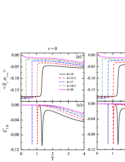
Figure 8: (a) and (b) Average $\langle S_{i}^{z}\sigma_{i+1}\rangle$ as a function of temperature. (c) and (d) Correlation function as a function of temperature. We assume fixed $J=100$, $J_{z}=24$, $J_{0}=-24$, and $\gamma=0.75$.

In Fig. 8, we show the Ising-Heisenberg spin pair average and the Ising-Heisenberg spin correlation function as a function of temperature, assuming the same set of parameters as in Fig. 6 and the values of $h$ as given in the legend of Fig. 8. Panel (a) illustrates the one-cell pair Ising-Heisenberg spin average ($r=0$, see Fig. 1). We observe here a noticeable jump around the pseudo-critical temperature $T_{p}$. The same quantity is displayed in panel (b) but now for $r=1$. In panel (c), the correlation function for one-cell Ising-Heisenberg spin pair is depicted, where we observe a strong depressing of the curves at pseudo-critical temperature $T_{p}$. Similarly in panel (d) the correlation function for $r=1$ is illustrated, and analogous behavior is observed. Therefore, all represented curves are entirely in agreement with the average of one-cell Ising-Heisenberg spin pair (80) and (81), as well as with the correlation function provided by Eq. (83).

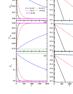
Figure 9: Correlation function decay with distance $r$ for $J=100$, $J_{z}=24$, $J_{0}=-24$, and $\gamma=0.75$. (a) For $\langle S_{i}^{z}S_{i+r}^{z}\rangle-\langle S_{i}^{z}\rangle\langle S_{i}^{z}\rangle$ against $r$. (b) Same as (a) but in logarithmic scale. (c) $\langle S_{i}^{z}\sigma_{i+r}\rangle-\langle S_{i}^{z}\rangle\langle\sigma_{i}\rangle$ against $r$. (d) Same as (c) but in logarithmic scale. (e) $\langle\sigma_{i}\sigma_{i+1}\rangle-\langle\sigma_{i}\rangle^{2}$ against $r$. (f) Same as (e) but in logarithmic scale.

Now we discuss the dependence of correlation functions on the interspin distance for several values of the magnetic field (and the corresponding pseudo-critical temperatures, see Fig. 4 and Table 1) which are shown in Fig. 9. From panel (a) it can be seen that the correlation function between Heisenberg-Heisenberg spins $C_{H}$ for low magnetic fields decays significantly with the increase of distance $r$, but while $h\rightarrow h_{c}$ ($h<h_{c}$) the decay becomes less significant, that means the correlations are strong even for far away spins. For example, for $h=18.5$ the correlation function becomes almost independent of distance $r$ up to $r\approx 2000$ (for more details see Table 2). The same plot is depicted in panel (b), but the correlation function is given in logarithmic scale here. It is simply a straight line with a slope $\ln\frac{\lambda_{-}}{\lambda_{+}}$, which is obviously negative because $\lambda_{-}<\lambda_{+}$. However, for $h=18.5$ this slopes is almost zero, while for lower magnetic fields the module of these slopes are large. Basically similar plots are shown in Fig. 9(c), (d) for distant mixed Ising and Heisenberg spins correlation functions $C_{IH}$; these correlation functions are negative. The distant pair Ising-Ising spin correlations $C_{I}$, illustrated in Fig. 9(e), (f), are positive and show the same behavior as the Heisenberg-Heisenberg correlation functions. Certainly, we also observe in all panels the zero correlation functions for $h>h_{c}$.

Table 2: Correlation function decay with distance. Here we report the ratio of $\frac{C(r)}{C(1)}$ in percent at the pseudo-critical temperature $T_{p}$. The three types of the correlation functions $C_{I}$, $C_{H}$ and $C_{IH}$ are denoted by $C$. We assume the fixed $xy$-anisotropy parameter $\gamma=\{0.7,0.75,0.8\}$.

$\gamma=0.7$
$h$	$r$	$\frac{C(r)}{C(1)}[\%]$
$10$	$20$	$50.15$
	$50$	$11.73$
	$100$	$2.75$
$11$	$50$	$53.35$
	$100$	$28.10$
	$300$	$2.16$
$12$	$500$	$53.05$
	$1000$	$28.11$
	$3000$	$2.21$
$12.5$	$1\negthickspace\times\negthickspace 10^{4}$	$69.78$
	$5\negthickspace\times\negthickspace 10^{4}$	$16.55$
	$1\negthickspace\times\negthickspace 10^{5}$	$2.74$

$\gamma=0.75$
$h$	$r$	$\frac{C(r)}{C(1)}[\%]$
$14$	$30$	$55.35$
	$100$	$13.28$
	$200$	$1.73$
$15.5$	$100$	$57.11$
	$200$	$32.43$
	$500$	$5.94$
$17$	$1000$	$63.86$
	$3000$	$26.02$
	$8000$	$2.76$
$18.5$	$1\negthickspace\times\negthickspace 10^{7}$	$55.05$
	$2\negthickspace\times\negthickspace 10^{7}$	$30.30$
	$7\negthickspace\times\negthickspace 10^{7}$	$1.53$

$\gamma=0.8$
$h$	$r$	$\frac{C(r)}{C(1)}[\%]$
$11$	$20$	$52.90$
	$50$	$19.36$
	$100$	$3.62$
$12.4$	$100$	$47.52$
	$200$	$22.42$
	$400$	$4.99$
$12.8$	$200$	$65.86$
	$500$	$35.09$
	$1000$	$12.29$
$13$	$2000$	$57.37$
	$4000$	$32.91$
	$1\negthickspace\times\negthickspace 10^{4}$	$6.21$

In Table 2 the ratio of correlation functions given by $\frac{C_{I}(r)}{C_{I}(1)}=\frac{C_{IH}(r)}{C_{IH}(1)}=\frac{C_{H}(r)}{C_{H}(1)}=\frac{C(r)}{C(1)}=\left(\frac{\lambda_{-}}{\lambda_{+}}\right)^{r-1}$ in percent is reported as a function of the assumed distance $r$ for various fixed magnetic fields and their corresponding pseudo-critical temperature $T_{p}$. Here we can see that as the magnetic field increases, the system shows strong correlation between distant spins. For $\gamma=0.75$ and $h=18.5$ the correlation function weakened compared to its nearest neighbor in about 50% for $r\approx 10^{7}$. Certainly, this is completely unexpected compared to the standard one-dimensional spin chain.

Additional plots of magnetizations and correlation functions for $\gamma=0.7$ and $\gamma=0.8$ are reported in Appendix B, where we observe similar behavior as for $\gamma=0.75$.

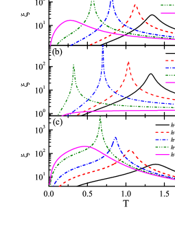
Figure 10: Correlation length against temperature, for the parameters considered in Fig. 2. (a) $\gamma=0.7$; (b) $\gamma=0.75$; (c) $\gamma=0.8$.

In addition, here we will discuss the correlation length $\xi(T)=\left(\ln\frac{\lambda_{+}}{\lambda_{-}}\right)^{-1}$, which characterizes exponential decay of correlations with distance. In Fig. 10(a) the correlation length $\xi(T)$ is depicted assuming $\gamma=0.7$ and the same parameters as considered in Fig. 2. We observe the peaks that are located at the pseudo-critical temperature $T_{p}$. The correlation length becomes extremely large, but remains finite at the pseudo-critical temperature $T_{p}$, the lower the temperature is, the larger the correlation length is. For higher temperatures the peak becomes smaller and wider. Analogously, Fig. 10(b) and Fig. 10(c) refer to $\gamma=0.75$ and $\gamma=0.8$; we observed here similar behavior.

In principle, the internal energy can be obtained using the relation

$$\mathcal{U}=\langle H\rangle=-\frac{\partial\lambda_{+}}{\partial\beta}.$$ (84)

Alternatively, the one-cell correlations are related to thermodynamics, since they determine the internal energy $\mathcal{U}$ of the spin system by

$$\mathcal{U}=\langle H\rangle= -J(1+\gamma)\langle S_{a}^{x}S_{b}^{x}\rangle-J(1-\gamma)\langle S_{a}^{y}S_{b}^{y}\rangle$$

$$-J_{z}\langle S_{a}^{z}S_{b}^{z}\rangle-4J_{0}\langle S^{z}\sigma\rangle-2h_{z}\langle S^{z}\rangle-h\langle\sigma\rangle.$$ (85)

Using the previous results (75), (79), (53) and (30), we find an equivalent result to that obtained from (84).

5 Conclusions

To summarize, we have examined the properties of the spin-$\frac{1}{2}$ Ising-XYZ diamond chain in the regime where the model shows pseudo-transitions and quasi-phases [12]. These pseudo-transitions are not true finite-temperature transitions but only sudden changes such as in the entropy, internal energy, and magnetization, which are quite similar to a first-order phase transition. While in some other thermodynamic quantities, in such as the specific heat, magnetic susceptibility, correlation length and correlation functions, sharp peaks arise which is also quite similar to a second-order phase transition. Therefore, this effect could be confused when interpreting experimental data and misinterpreted as a true phase transition.

A simple way to understand the presence of quasi-phases and pseudo-critical temperature could be the mapping of the original spin-$\frac{1}{2}$ Ising-XYZ diamond chain onto a simple effective ferromagnetic ($J_{\mathrm{eff}}>0$) Ising model with effective magnetic field $h_{\mathrm{eff}}$ through a decoration transformation. The zero effective magnetic field $h_{{\rm{eff}}}(T_{p})=0$ when $\bar{w}_{0}\rightarrow 0$ indicates the presence of the so-called pseudo-critical temperature $T_{p}$ leading to a simultaneous flip of all Ising spins. Previously in Ref. [12] an equivalent condition $w_{1}=w_{-1}$ when $\bar{w}_{0}\rightarrow 0$ was considered.

Hence, we analyzed the quasi-phase diagram at low temperatures and determined the region of parameters where the pseudo-transitions may occur. Here we consider a detailed investigation of Ising spin and Heisenberg spin magnetization, as well as the pair correlation function with arbitrary distance. Basically in this model we have three types of correlation functions: Ising-Ising spin correlation function $C_{I}$, Ising-Heisenberg spin correlation functions $C_{IH}$, and Heisenberg-Heisenberg spin correlation functions $C_{H}$. The magnetizations of the Ising and Heisenberg spin illustrate the presence of a substantial change in magnetization near the pseudo-critical temperature. Likewise, all correlation functions were also focused around the pseudo-critical temperature, where we observed prominent peaks at pseudo-critical temperature and this effect is supported by the analytical results. It is also worth mentioning that the correlation function at pseudo-critical temperature $T_{p}$ has large correlation length. For example, for $\gamma=0.8$ and the parameters considered in Fig. 2 with magnetic field bit below the critical magnetic field ($h<h_{c}$), i.e., $h=18.5$, the correlation functions become almost insensitive to $r$ for up to $r\sim 10^{6}$.

Appendix A Heisenberg spin matrices

In this appendix we give in detail the elements of some important matrices. First, we consider for the Heisenberg spin at site $a$ (see Fig. 1):

$$\hat{\mathbf{s}}_{a}^{z}=\frac{1}{2}\left(\begin{array}[]{cccc}-\cos(2\theta_{\mu})&0&0&-\sin(2\theta_{\mu})\\ 0&0&-1&0\\ 0&-1&0&0\\ -\sin(2\theta_{\mu})&0&0&\cos(2\theta_{\mu})\end{array}\right),$$ (86)

where $\tan(2\theta_{\mu})=\frac{J\gamma}{2J_{0}\mu+2h}$ and $0<\theta_{\mu}<\pi$. Similarly, the other components become

$$\hat{\mathbf{s}}_{a}^{x}=\frac{1}{2}\left(\begin{array}[]{cccc}0&\cos\hat{\theta}_{\mu}&-\sin\hat{\theta}_{\mu}&0\\ \cos\hat{\theta}_{\mu}&0&0&\sin\hat{\theta}_{\mu}\\ -\sin\hat{\theta}_{\mu}&0&0&\cos\hat{\theta}_{\mu}\\ 0&\sin\hat{\theta}_{\mu}&\cos\hat{\theta}_{\mu}&0\end{array}\right),$$ (87)

by $\hat{\theta}_{\mu}$ we define conveniently $\hat{\theta}_{\mu}=\theta_{\mu}+\frac{\pi}{4}$, and

$$\hat{\mathbf{s}}_{a}^{y}=\frac{i}{2}\left(\begin{array}[]{cccc}0&\sin\hat{\theta}_{\mu}&-\cos\hat{\theta}_{\mu}&0\\ -\sin\hat{\theta}_{\mu}&0&0&\cos\hat{\theta}_{\mu}\\ \cos\hat{\theta}_{\mu}&0&0&\sin\hat{\theta}_{\mu}\\ 0&-\cos\hat{\theta}_{\mu}&-\sin\hat{\theta}_{\mu}&0\end{array}\right).$$ (88)

Second, we obtain similarly for the Heisenberg spin at site $b$ (see Fig. 1):

$$\hat{\mathbf{s}}_{b}^{z}=\frac{1}{2}\left(\begin{array}[]{cccc}-\cos(2\theta_{\mu})&0&0&-\sin(2\theta_{\mu})\\ 0&0&1&0\\ 0&1&0&0\\ -\sin(2\theta_{\mu})&0&0&\cos(2\theta_{\mu})\end{array}\right),$$ (89)

$$\hat{\mathbf{s}}_{b}^{x}=\frac{1}{2}\left(\begin{array}[]{cccc}0&\cos\hat{\theta}_{\mu}&\sin\hat{\theta}_{\mu}&0\\ \cos\hat{\theta}_{\mu}&0&0&\sin\hat{\theta}_{\mu}\\ \sin\hat{\theta}_{\mu}&0&0&-\cos\hat{\theta}_{\mu}\\ 0&\sin\hat{\theta}_{\mu}&-\cos\hat{\theta}_{\mu}&0\end{array}\right),$$ (90)

and

$$\hat{\mathbf{s}}_{b}^{y}=\frac{i}{2}\left(\begin{array}[]{cccc}0&\sin\hat{\theta}_{\mu}&\cos\hat{\theta}_{\mu}&0\\ -\sin\hat{\theta}_{\mu}&0&0&\cos\hat{\theta}_{\mu}\\ -\cos\hat{\theta}_{\mu}&0&0&-\sin\hat{\theta}_{\mu}\\ 0&-\cos\hat{\theta}_{\mu}&\sin\hat{\theta}_{\mu}&0\end{array}\right).$$ (91)

Therefore, $\tilde{w}_{1}^{z}$ is given more explicitly

$$\tilde{w}_{1}^{z}= \frac{h_{z}+J_{0}}{\Delta_{1}}{\rm e}^{\beta\left(\frac{h}{2}+\frac{J_{z}}{4}\right)}\sinh(\beta\Delta_{1})\cos^{2}\phi+\frac{h_{z}}{\Delta_{0}}{\rm e}^{\frac{\beta J_{z}}{4}}\sinh(\beta\Delta_{0})\sin(2\phi)$$

$$+\frac{h_{z}-J_{0}}{\Delta_{-1}}{\rm e}^{\beta\left(-\frac{h}{2}+\frac{J_{z}}{4}\right)}\sinh(\beta\Delta_{-1})\sin^{2}\phi.$$ (92)

Using the the relation (26) and assuming $\bar{w}_{0}\rightarrow 0$, we find the following expansions up to order $\bar{w}_{0}^{2}$,

$$\cos^{2}\phi= \frac{1}{2}\left(1+\frac{w_{1}-w_{-1}}{B}\right)=\frac{1}{2}\left[1+\frac{w_{1}-w_{-1}}{|w_{1}-w_{-1}|}\left(1-2\bar{w}_{0}^{2}+\mathcal{O}\left(\bar{w}_{0}^{4}\right)\right)\right],$$ (93)

$$\sin^{2}\phi= \frac{1}{2}\left(1-\frac{w_{1}-w_{-1}}{B}\right)=\frac{1}{2}\left[1-\frac{w_{1}-w_{-1}}{|w_{1}-w_{-1}|}\left(1-2\bar{w}_{0}^{2}+\mathcal{O}\left(\bar{w}_{0}^{4}\right)\right)\right].$$ (94)

Appendix B Additional correlation quantities

Here we report additional plots concerning magnetizations and correlation functions, see Fig. 11. Mainly we observe similar behavior as it was discussed in the main text. The only difference we worth to mention would be that this pseudo-critical temperature occurs between two quasi-phases: For $\gamma=0.7$ the pseudo-transition occurs between $qFI$ and $qMF_{0}$, whereas for $\gamma=0.8$ the pseudo-transition occurs between $qMF_{0}$ and $qMF_{2}$.

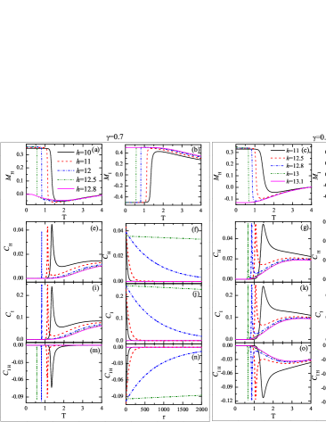
Figure 11: The left block of columns corresponds to fixed $\gamma=0.7$ and fixed $J=100$, $J_{z}=24$, and $J_{0}=-24$. (a) Heisenberg spin magnetization as a function of temperature. (b) Ising spin magnetization as a function of temperature. (e), (f) Heisenberg spin correlation functions. (i), (j) Ising spin correlation functions. (m), (n) Ising-Heisenberg spin correlation functions. Similarly, the right block of columns corresponds to fixed $\gamma=0.8$. (c), (d) magnetizations as a function of temperature. (g), (h) Heisenberg spin correlation functions. (k), (l) Ising spin correlation functions. (o), (p) Ising-Heisenberg spin correlation functions.

References

[1] J. A. Cuesta and A. Sánchez, J. Stat. Phys.
115, 869 (2004).
[2] F. J. Dyson, Comm. Math. Phys. 12,
212 (1969).
[3] J. A. Cuesta and A. Sánchez, J. Phys. A 35,
2373 (2002).
[4] S. Ares, J. A. Cuesta, A. Sánchez, and R. Toral,
Phys. Rev. E 67, 046108 (2003).
[5] X. Ma, S. Cambré, W. Wenseleers, S. K. Doorn,
and H. Htoon, Phys. Rev. Lett. 118, 027402 (2017).
[6] L. Ferrari and G. Russo, Let. Nuov. Cim.
43, 319 (1985).
[7] J. Torrico, M. Rojas, S. M. de Souza,
O. Rojas, and N. S. Ananikian, Europhys. Lett. 108, 50007
(2014).
[8] J. Torrico, M. Rojas, S. M. de Souza,
and O. Rojas, Phys. Lett. A 380, 3655 (2016).
[9] L. Gálisová and J. Strečka, Phys. Rev.
E 91, 022134 (2015).
[10] O. Rojas, J. Strečka, and S. M. de Souza,
Solid State Commun. 246, 68 (2016).
[11] J. Strečka, R. C. Alecio, M. Lyra,
and O. Rojas, J. Magn. Magn. Matter 409, 124 (2016).
[12] S. M. de Souza and O. Rojas, Solid State
Commun. 269, 131 (2018).
[13] M. E. Fisher, Phys. Rev. 113, 969
(1959).
[14] I. Syozi, in Phase Transitions and Critical
Phenomena, Vol. 1, edited by C. Domb and M. S. Green (Academic
Press, New York, 1972).
[15] O. Rojas, J. S. Valverde, and S. M. de Souza,
Physica A 388 (2009) 1419.
[16] J. Strečka, Phys. Lett. A, 374
(2010) 3718; J. Strečka, On the Theory of Generalized
Algebraic Transformations (LAP LAMBERT Academic Publishing, Saarbrücken,
2010) [arXiv:1008.2071].
[17] S. Bellucci and V. Ohanyan, Eur. Phys. J.
B 86, 446 (2013).