A dessin on the base: a description of mutually non-local 7-branes without using branch cuts

Abstract

We consider the special roles of the zero loci of the Weierstrass invariants $g_{2}(\tau(z))$, $g_{3}(\tau(z))$ in F-theory on an elliptic fibration over $\hbox{\mybbsmall P}^{1}$ or a further fibration thereof. They are defined as the zero loci of the coefficient functions $f(z)$ and $g(z)$ of a Weierstrass equation. They are thought of as complex co-dimension one objects and correspond to the two kinds of critical points of a dessin d’enfant of Grothendieck. The $\hbox{\mybbsmall P}^{1}$ base is divided into several cell regions bounded by some domain walls extending from these planes and D-branes, on which the imaginary part of the $J$-function vanishes. This amounts to drawing a dessin with a canonical triangulation. We show that the dessin provides a new way of keeping track of mutual non-localness among 7-branes without employing unphysical branch cuts or their base point. With the dessin we can see that weak- and strong-coupling regions coexist and are located across an $S$-wall from each other. We also present a simple method for computing a monodromy matrix for an arbitrary path by tracing the walls it goes through.

I Introduction

The importance of F-theory Vafa ; MV1 ; MV2 in modern particle physics model building cannot be too much emphasized. The $SU(5)$ GUT, which can naturally explain the apparently complicated assignment of hypercharges to quarks and leptons, is readily achieved in F-theory. Another virtue of F-theory is that it can yield matter in the spinor representation of $SO(10)$, into which all the quarks and leptons of a single generation are successfully incorporated, and which cannot be achieved in pure D-brane models. These features are shared by $E_{8}\times E_{8}$ heterotic models, but F-theory models have an advantage in that they may evade the issue of the relation between the GUT and Planck scales in heterotic string theory first addressed in Witten96 . Also, the Yukawa couplings perturbatively forbidden in D-brane models Yukawaforbidden1 ; Yukawaforbidden2 can be successfully generated in F-theory.

Almost ten years after the first development in F-theory, there was much progress in the studies of local models of F-theory (See DonagiWijnholt ; BHV ; BHV2 ; DonagiWijnholt2 ; HKTW ; DWHiggsBundles ; localmodel1 ; localmodel2 ; localmodel3 ; localmodel4 for an incomplete list.). In this class of theories, one basically considers a supersymmetric gauge theory on a stack of 7-branes in F-theory, whose coalescence is supposed to give rise to a gauge symmetry depending on the fiber type in the Kodaira classification. In particular, if the fiber type is either $IV^{*}$, $III^{*}$ or $II^{*}$, the gauge symmetry will be $E_{6}$, $E_{7}$ or $E_{8}$, respectively, and then the brane was called an exceptional brane BHV .

The fiber type of such a codimension-one singularity can be labeled by the (conjugacy class of the) $SL(2,\hbox{\mybb Z})$ monodromy around the fiber. It was shown that all the types of Kodaira fibers can be represented by some product of monodromies of a basic set of 7-branes: A=D-brane, B=$(1,1)$-brane and C=(1,$-1$)-brane GHZ ; DZ ; DHIZ , as shown in Table in Appendix . The relation between the resolution of the singularity and the gauge symmetry on a coalescence of 7-branes has been clearly explained by using string junctions. String junctions are also useful to describe chiral matter tani , non-simply-laced Lie algebras BonoraSavelli , the Mordell-Weil lattice of a rational elliptic surface FYY and deformations of algebraic varieties GHS ; GHS2 .

From the table one can see that the singular fibers of the exceptional type consist of a B-brane and two C-branes in addition to the ordinary D($=$A)-branes. Thus, in this algebraic approach, the exceptional branes are seen to emerge due to the coalescence of these B- and C-branes which are distinct from D-branes. From a geometrical point of view, however, these branes are just the zero loci of the discriminant of a Weierstrass equation and there are no a priori differences from each other; they all are locally D-branes.

In this paper, we consider the special roles of the zero loci of the Weierstrass invariants $g_{2}(\tau(z))$, $g_{3}(\tau(z))$ in F-theory on an elliptic fibration over $\hbox{\mybb P}^{1}$, or a further fibration thereof. They are defined as the zero loci of the coefficient functions $f(z)$ and $g(z)$ of a Weierstrass equation. They are thought of as complex co-dimension one objects, and we call them “elliptic point planes”.

In fact, mathematically, our construction amounts to drawing a “dessin d’enfant” of Grothendieck on the $\hbox{\mybb P}^{1}$ base with a canonical triangulation. We show that this drawing provides a new way of keeping track of mutual non-localness among 7-branes in place of the conventional ABC 7-brane description. In our approach, all the discriminant loci are treated democratically, and with this “dessin” we can see that weak- and strong-coupling regions coexist and are located across an $S$-wall from each other. We also present a simple method for computing a monodromy matrix for an arbitrary path by tracing the walls it goes through. The method for studying monodromies by tracing the contours on the $J(\tau)$-plane was developed long time ago by Tani tani .

This paper is organized as follows: In section 2, we introduce the basic setup of this paper, including the motivations and definitions of the elliptic point planes, the domain walls extended from them, and the cell region decomposition of the $\hbox{\mybb P}^{1}$ base of the elliptic fibration. The various definitions of the new notions and objects are summarized as a mini-glossary at the end of this section. In section 3, we briefly explain what is a “dessin d’enfant” and the relation to our present construction. In section 4, we discuss the basic properties of the two kinds of elliptic point planes, the $f$-plane and the $g$-plane. In section 5, we present a new method for computing the monodromy by drawing the dessin. In the final section we conclude with a summary of our findings. Appendix A contains a table of fiber types of the Kodaira classification. The plots presented in this paper have been generated with the aid of Mathematica.

II What is an elliptic point plane?

Consider a Weierstrass equation

$$y^{2}=x^{3}+fx+g,$$ (1)

where $y$, $x$, $f$ and $g$ are sections of an ${\cal O}(3)$, an ${\cal O}(2)$, an ${\cal O}(4)$ and an ${\cal O}(6)$ bundle over the base $\hbox{\mybb P}^{1}$. This is a rational elliptic surface, which we regard as one of the two rational elliptic surfaces arising in the stable degeneration limit of a K3 surface. It may also be thought of as the total space of a Seiberg-Witten curve (with the “$u$”-plane being the base) of an ${\cal N}=2$ $SU(2)$ gauge theory or an E-string theory. In an affine patch of $\hbox{\mybb P}^{1}$ with the coordinate $z$, the coefficient functions $f(z)$ and $g(z)$ are a 4th and a 6th order polynomial in $z$.

As is well known, the modulus $\tau$ of the elliptic fiber of (1) is given by the implicit function:

$$J(\tau) = \frac{4f^{3}}{4f^{3}+27g^{2}},$$ (2)

where $J$ is the elliptic modular function. The denominator of the right hand side

$$\Delta \equiv 4f^{3}+27g^{2}$$ (3)

is called the discriminant. Near its zero locus $z=z_{i}$, $\mbox{Im}\tau$ goes to $\infty$ (if one has chosen the “standard” fundamental region) for generic (that is, nonzero) $f$ and $g$. Examining the behavior of $J(\tau)$ around $\infty$, we find

$$\tau(z) = \frac{1}{2\pi i}\log(z-z_{i})\left(\text{const.}+O(z-z_{i})\right),$$ (4)

which implies the existence of a D7-brane at each discriminant locus.

On the other hand, since a locus of $f(z)=0$ or $g(z)=0$ alone does not mean $\Delta=0$, it is not a D-brane. However, if the loci of $f(z)=0$ and $g(z)=0$ are present together with a D-brane, they play a significant role in generating a $(p,q)$-7-brane by acting $SL(2,\hbox{\mybb Z})$ conjugate transformations on a D-brane or as components of an orientifold plane, as we show below. In this paper, we will collectively call the loci of $f(z)=0$ and $g(z)=0$ “elliptic point planes”.

Elliptic point planes consist of two types, the loci of $f(z)=0$ and $g(z)=0,$ which have different properties. In this paper, we call the locus of $f(z)=0$ an $f\!\!=\!0$ locus plane, or an $f$-plane for short, and that of $g(z)=0$ a $g\!=\!0$ locus plane, or a $g$-plane for short.

At the location of an $f$-plane, the value of the $J$-function is

$$J(\tau) = \frac{4f^{3}}{4f^{3}+27g^{2}}~{}=~{}0,$$ (5)

which corresponds to $\tau=e^{\frac{2\pi i}{3}}$. On the other hand, at the position of a $g$-plane ,

$$J(\tau) = \frac{4f^{3}}{4f^{3}+27g^{2}}~{}=~{}1,$$ (6)

so this implies $\tau=i$. In their neighborhoods, $J(\tau)$ is expanded as

$$J(\tau) = \frac{1}{3!}J^{\prime\prime\prime}(e^{\frac{2\pi i}{3}})(\tau-e^{\frac{2\pi i}{3}})^{3}+O\left((\tau-e^{\frac{2\pi i}{3}})^{4}\right),$$ (7)

$$J(\tau) = 1-\frac{12K\left(\frac{1}{\sqrt{2}}\right)^{4}}{\pi^{2}}(\tau-i)^{2}+O\left((\tau-i)^{3}\right),$$ (8)

where $K(k)$ is the complete elliptic integral of the first kind

$$K(k) = \int_{0}^{\frac{\pi}{2}}\frac{d\theta}{\sqrt{1-k^{2}\sin^{2}\theta}}.$$ (9)

Thus $\tau=e^{\frac{2\pi i}{3}}$ is a triple zero of $J(\tau)$ and $\tau=i$ is a double zero of $J(\tau)-1$.

Suppose that $z=0$ is a locus of $f=0$. Since

$$J(\tau(z)) = \frac{4f(z)^{3}}{4f(z)^{3}+27g(z)^{2}},$$ (10)

$J(\tau(z))$ is $O(z^{3})$ at $z=0$. So (7) shows that $\tau-e^{\frac{2\pi i}{3}}$ is $O(z)$ there, implying that the monodromy is trivial around the locus of $f$. Similarly, if $z=0$ is a locus of $g=0$, $J(\tau(z))-1$ is now $O(z^{2})$. Comparing this with (8), we see that $\tau(z)-i$ is also $O(z)$, and hence there is no monodromy around the locus of $g=0$, either.

However, this is not the end of the story. Figure 2 shows the various choices of fundamental regions of the modulus $\tau$ and the corresponding complex plane as its image mapped by the $J$-function. From this we can see that if one goes around $\tau=e^{\frac{2\pi i}{3}}$ once on the upper half plane, one goes through three different fundamental regions to get back to the original position. Likewise if one goes around $\tau=i$, one undergoes two different fundamental regions. Thus an $f$-plane is a complex codimension-one submanifold at which three different regions on the $z$-plane corresponding to different fundamental regions meet, while a $g$-plane is similarly the place where two different regions meet. The regions on the $z$-plane corresponding to different fundamental regions are bounded by real codimension-one domain walls which consist of the zero loci of the imaginary part of the $J$-function.

Furthermore, each region on the $z$-plane corresponding to a definite fundamental region is divided by a domain wall

$$\{\tau|~{}\mbox{Im}J(\tau)=0,~{}\mbox{Re}J(\tau)>1\}$$ (11)

(a dashed green line) into two regions $\mbox{Im}J(\tau)>0$ and $\mbox{Im}J(\tau)<0$.

On the other hand, a D-brane resides at a discriminant locus $\Delta=0$, from which two domain walls $\{\tau|~{}\mbox{Im}J(\tau)=0,~{}\mbox{Re}J(\tau)<0\}$ (a green line) and $\{\tau|~{}\mbox{Im}J(\tau)=0,~{}\mbox{Re}J(\tau)>1\}$ (a dashed green line) extend out into the bulk $z$ space ($\hbox{\mybb P}^{1}$) (Fig.1).

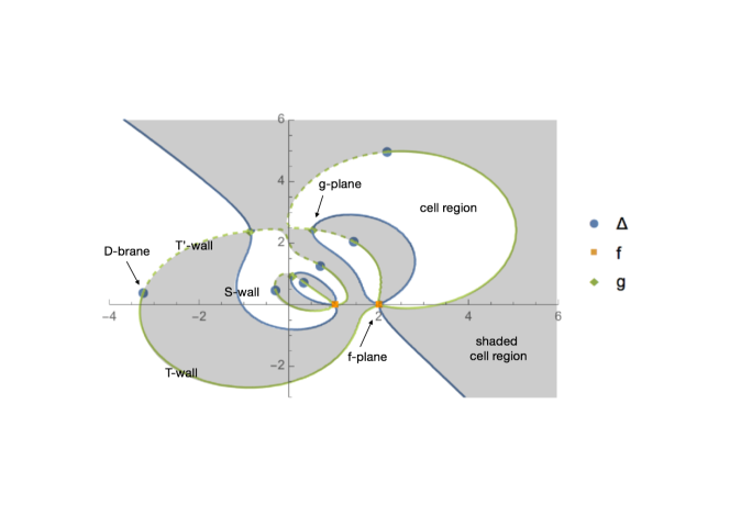
Figure 1: An example configuration of D-branes, elliptic point planes and the cell regions bounded by the domain walls extended from them. D-branes are located at the loci of $\Delta=0$, while elliptic point planes are at the loci of $f=0$ and $g=0$. In this example we can see two $f$-planes at $z=1,2$, three $g$-planes and six D-branes. (This figure is depicted for the Weierstrass equation (1) for $f$ and $g$ (50) with $\epsilon=0.9$.)

Since the value of $J$ is $\infty$ at a discriminant locus for generic (i.e. nonzero) values of $f$ and $g$, D-branes can never, by definition, touch nor pass through (a non-end point of) the domain walls because $\mbox{Im}J(\tau)$ must vanish at the domain walls.

In this way, the $z$-space ($=\hbox{\mybb P}^{1}$) is divided into several “cell regions”, which correspond to different fundamental regions in the preimage of the $J$-function, by the domain walls extended from the elliptic point planes (=$f$-planes and $g$-planes) and D-branes (Fig.1). In particular, $f$-planes and $g$-planes extend the domain walls

$$\{\tau|~{}\mbox{Im}J(\tau)=0,~{}0<\mbox{Re}J(\tau)<1\}$$ (12)

(blue lines), and crossing through this wall implies that the type IIB coupling locally gets S-dualized (if starting from the standard choice of the fundamental region) (Fig.2). Then there is a difference in monodromies between when one goes around a D-brane within a single cell region bounded by some domain walls and when one first crosses through a domain wall, moves around a D-brane and then crosses back through the wall again to the original position; they are different by an $SL(2,\hbox{\mybb Z})$ conjugation. This is what’s happening in what has been called a “B-brane” or a “C-brane” in the discussions of string junctions. That is, while the monodromy matrix is necessarily

$$T = \left(\begin{array}[]{cc}1&1\\ 0&1\end{array}\right)$$ (15)

as long as the reference point is chosen to be in the standard fundamental region, a non-trivial (non-D-brane) $(p,q)$-brane arises if the monodromy is measured by going back and forth between regions corresponding to different fundamental regions in the preimage upper-half plane.

   

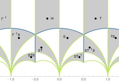
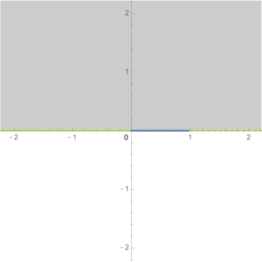
Figure 2: Left: The upper half plane and various fundamental regions. The shaded regions are the regions in which the imaginary part of the image of the $J$-function ${\rm Im}J(\tau)$ is positive. The symbol in each fundamental region (such as ${\rm Id}$, $T$, $S,\ldots$) is the group element of $SL(2,\hbox{\mybb Z})$ that maps the standard fundamental region to the fundamental region specified by the symbol. Right: The images of the $J$-function (= the whole complex plane). The green, blue and dashed green lines correspond to the respective boundary components of any one half of (the closure of) the fundamental regions.

We would like to emphasize here that such a local $S$ transformation never takes place without these “elliptic point planes” (=$f$-planes and $g$-planes). If it were not for elliptic point planes but there are only D-branes, the domain walls extended from them are only the ones

$$\{\tau|~{}\mbox{Im}J(\tau)=0,~{}\mbox{Re}J(\tau)<0\}$$ (16)

(green lines) and

$$\{\tau|~{}\mbox{Im}J(\tau)=0,~{}\mbox{Re}J(\tau)>1\}$$ (17)

(dashed green lines). So crossing through these walls only leads to a $T$ transformation which commutes with the original monodromies of D-branes.

In the discussion below, we refer to the domain wall (16) (a green lines) as $T$-wall and the one (17) (a dashed green line) as $T^{\prime}$-wall, whereas we call the type of domain wall (12) (a blue line) $S$-wall.

To conclude this section we summarize the definitions of the new objects and notions introduced in this section as a mini-glossary.

Mini-glossary
$f$-plane A (complex) co-dimension-1 object corresponding to a zero locus of $f(z)$ in the Weierstrass form on the $z$-plane. Represented by a small square in the figures.
$g$-plane A (complex) co-dimension-1 object corresponding to a zero locus of $g(z)$ in the Weierstrass form on the $z$-plane. Represented by a small $45^{\circ}$-rotated square in the figures.
elliptic point plane The collective name for $f$-planes and $g$-planes.
$T$-wall A (real) co-dimension-1 object (domain wall) corresponding to a zero locus of ${\rm Im}J$ with ${\rm Re}J<0$, extending from a D-brane and a $f$-plane. Represented by a green line.
$T^{\prime}$-wall A (real) co-dimension-1 object (domain wall) corresponding to a zero locus of ${\rm Im}J$ with ${\rm Re}J>1$, extending from a D-brane and a $g$-plane. Represented by a dashed green line.
$S$-wall A (real) co-dimension-1 object (domain wall) corresponding to a zero locus of ${\rm Im}J$ with $0<{\rm Re}J<1$, extending from a $f$-plane and a $g$-plane. Represented by a blue line.
cell region A closed region on the $z$-plane ($\hbox{\mybb P}^{1}$ base of the elliptic fibration) bounded by the $T$-, $T^{\prime}$- and $S$-walls. Each cell region corresponds to either half of the (closure of the) fundamental region with ${\rm Im}J>0$ or ${\rm Im}J<0$ of the fiber modulus.
shaded cell region The cell region corresponding to the (closure of the) half fundamental region with ${\rm Im}J>0$ (Figure 1).

III Relation to “dessin d’enfant” of Grothendieck

In fact, the construction in the previous section is nothing but drawing a “dessin d’enfant” of Grothendieck Grothendieck , known in mathematics, on the $\hbox{\mybb P}^{1}$ base with a canonical triangulation. A dessin d’enfant, meaning a drawing of a child, is a graph consisting of some black points, white points and lines connecting these points, drawn according to a special rule. To demonstrate the rule, let us consider, for example, a function LandoZvonkin :

$$F(x)=-\frac{(x-1)^{3}(x-9)}{64x}=1-\frac{(x^{2}-6x-3)^{2}}{64x},$$ (18)

where $x\in\hbox{\mybb P}^{1}$. $F$ is a map from $\hbox{\mybb P}^{1}$ to $\hbox{\mybb P}^{1}$. At almost everywhere on $\hbox{\mybb P}^{1}$, $F$ is a homeomorphism, sending a small disk to another in a one-to-one way. However, $F$ maps a small disk centered at $x=1$ to one centered at $F=0$ in a three-to-one way. Similarly, $F$ is a two-to-one map from a small disk centered at $x=3\pm 2\sqrt{3}$ to one centered at $F=1$. The points $x=1,3\pm 2\sqrt{3}$ are said critical points, and the corresponding values of $F$ are said critical values. If the map from the neighborhood around a critical point to another around the corresponding critical value is $k$-to-one, we say that the ramification index of the critical point is $k$.

Now the rule to draw the dessin associated with (18) is as follows: Place a black point at every preimage of $0$, and a while point at every preimage of $1$. Next draw lines at preimages of the line segment $[0,1]$. The result is shown in FIG.3(a):

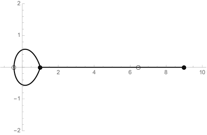
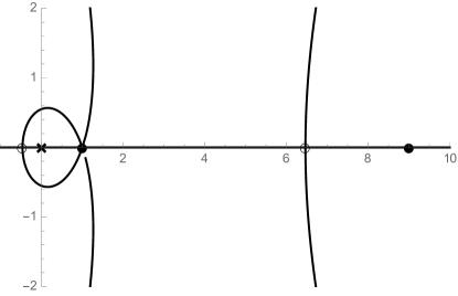
Figure 3: (a)(left panel): The dessin for (18). (b)(right panel): The triangulated dessin. $\times$ represents an $\infty$ point. The extra lines have been drawn at the preimages of the segment $[-\infty,0]$ and $[1,\infty]$. The other $\infty$ point is not shown in this figure as it is infinitely far away.

The equation (18) induces a branched covering over $\hbox{\mybb P}^{1}$. Treating this graph as a combinatorial object, one can reproduce the information of the branched covering as follows: One first adds a point $\infty$ to each region of the dessin. One then connects each $\infty$ with lines to the black or white points as many times as they appear on the boundary of the region. This yields a triangulation of the dessin. Assigning either the upper- or the lower-half plane to each triangle depending on the ordering of $0$, $1$, $\infty$, and glueing these half planes together, one obtains a branched covering equivalent to the original one LandoZvonkin .

In the present case, the equation (10) defines a Belyi function, a holomorphic function whose critical values are only $0$, $1$ and $\infty$ and nothing else. The black and white points in the dessin shown in FIG.3(a) correspond to the $f$-planes and $g$-planes. The points $\infty$ added in the triangulation of the dessin are D-branes. The lines shown in FIG.3(a) are the $S$-walls, while the lines connecting the $\infty$ points and the black or white points drawn in the triangulation are the $T$- and $T^{\prime}$-walls.

What is special about (10) is that it induces a local homeomorphism between the $\hbox{\mybb P}^{1}$ base and the upper-half plane. Indeed, as we saw in the previous section, the correspondence is one-to-one everywhere, even in the vicinity of the elliptic orbits $\tau=e^{\frac{2\pi i}{3}}$ and $i$. This is so because the $J=0$ ($f=0$) points are always critical points with ramification index three, and the $J=1$ ($g=0$) points are always with ramification index two. In this paper, we treat the dessin not as just a combinatorial graph, but draw the $\infty$ points and the triangulating lines (the $T$- and $T^{\prime}$-walls) also as preimages of the $J$-function, as shown in FIG.3(b). The special feature of (10) then allows us to use the (triangulated) dessin as a convenient tool to compute monodromies, as we see below.

IV Basic properties of elliptic point planes

IV.1 Basic properties of $f$-planes

As we defined in the previous sections, there are two kinds of elliptic point planes: $f$-planes and $g$-planes. In this section we describe the basic properties of $f$-planes.

As the name indicates, $f$-planes are the loci where the function $f$ vanishes. As we saw in the previous section, these are the places where the $J$-function vanishes and $\tau$ becomes $e^{\frac{2\pi i}{3}}$ (or its $SL(2,\hbox{\mybb Z})$ equivalents).

As we saw in the previous section, the expansion of $J(\tau)$ near $\tau=e^{\frac{2\pi i}{3}}$ is given by (7). If there is an $f$-plane at $z=0$, $f=0$ there, yielding

$$f(z) = f_{41}z+f_{42}z^{2}+\cdots,$$ (19)

$$g(z) = g_{60}+g_{61}z+g_{62}z^{2}+\cdots,$$ (20)

where $f_{4i}$, $g_{6j}$ are constants with indices running over $i=1,\ldots,8$ and $j=1,\ldots,12$ for a K3 surface and $i=1,\ldots,4$ and $j=1,\ldots,6$ for a rational elliptic surface. Since

$$\frac{4f^{3}}{4f^{3}+27g^{2}} = \frac{4f_{41}^{3}}{27g_{60}^{2}}z^{3}(1+O(z)),$$ (21)

$\tau(z)$ asymptotically approaches

$$\tau(z) = e^{\frac{2\pi i}{3}}+\frac{2f_{41}}{(9g_{60}^{2}J^{\prime\prime\prime}(e^{\frac{2\pi i}{3}}))^{\frac{1}{3}}}z$$ (22)

as $z\rightarrow 0$. Therefore, $\tau$ is regular near $z=0$, and hence an $f$-plane does not carry D-brane charges.

Parameterize a small circle around $z=0$ by $z=\epsilon e^{i\theta}$ $(\epsilon>0)$, then if one goes around along it once, so does $\tau$ once around $e^{\frac{2\pi i}{3}}$ along a small circle with a radius $\epsilon\left|\frac{2f_{41}}{(9g_{60}^{2}J^{\prime\prime\prime}(e^{\frac{2\pi i}{3}}))^{\frac{1}{3}}}\right|$. Thus, although the monodromy around an $f$-plane is trivial, one passes through the boundary of the half-fundamental region six times on the upper-half plane as one goes once around an $f$-plane. Since the neighborhoods of $z=0$ and $\tau=e^{\frac{2\pi i}{3}}$ are homeomorphic, the neighborhood of $z=0$ around an $f$-plane is also divided into six cell regions corresponding to different half-fundamental regions. The six domain walls separating these cell regions consist of three $S$-walls (blue) with $(0<\mbox{Re}J(\tau)<1)$ and three $T$-walls (green) $(\mbox{Re}J(\tau)<0)$, which are extended alternately from the $f$-plane, forming a locally $\hbox{\mybb Z}_{3}$-symmetric configuration.

On the upper-half plane, if one starts from the standard fundamental region and passes through preimages (of the $J$-function) of a $T$-wall (green) and an $S$-wall (blue) to go to the $SL(2,Z)$ equivalent point, then the $SL(2,\hbox{\mybb Z})$ transformation mapping the original point to the final point is $T^{-1}S$. Further, if one crosses through preimages of a $T$-wall (green) and an $S$-wall (blue) again, the transformation to the final $SL(2,Z)$ equivalent point is $(T^{-1}S)^{2}=-ST\sim ST$ (as $PSL(2,\hbox{\mybb Z})$) .

Since

$$(T^{-1}S)^{3} = 1,$$ (23)

$T^{-1}S$ generates a $\hbox{\mybb Z}_{3}$ group, which is the isotropy group of the elliptic point $\tau=e^{\frac{2\pi i}{3}}$. It is easy to show that this $T^{-1}S$ transformation acts on the neighborhood of this point as a $\frac{2\pi i}{3}$ rotation. Therefore, the configuration of $\tau$ near an $f$-plane is locally invariant under the simultaneous actions of the spacial $\hbox{\mybb Z}_{3}$ rotation and the $\hbox{\mybb Z}_{3}$ $SL(2,\hbox{\mybb Z})$ transformation. The metric near an $f$-plane is locally $\hbox{\mybb Z}_{3}$ invariant.

IV.2 Basic properties of $g$-planes

Likewise, the expansion of $J(\tau)$ around $\tau=i$ is given by (8). Let a $g$-plane be at $z=0$ this time. $f(z)$ and $g(z)$ are expanded as

$$f(z) = f_{40}+f_{41}z+f_{42}z^{2}+\cdots,$$ (24)

$$g(z) = g_{61}z+g_{62}z^{2}+\cdots.$$ (25)

Since

$$\frac{4f^{3}}{4f^{3}+27g^{2}} = 1-\frac{27g_{61}^{2}}{4f_{40}^{3}}z^{2}(1+O(z)),$$ (26)

$\tau(z)$ approaches

$$\tau(z) = i+\frac{3i\pi^{\frac{1}{2}}g_{61}}{4K(\frac{1}{\sqrt{2}})^{2}f_{40}^{\frac{3}{2}}}z$$ (27)

as $z\rightarrow 0$. Thus $\tau$ is again regular near a $g$-plane, therefore a $g$-plane does not have D-brane charges, either. The monodromy around a $g$-plane is also trivial, although if one goes around it, one will be passing through the $S$-walls (blue lines) and the $T^{\prime}$-walls (dashed green lines) alternately, twice for each.

Suppose that on the upper-half plane one starts from an arbitrarily given point near $\tau=i$ in the standard fundamental region with $\mbox{Re}\tau<0$ and goes through the preimages of an $S$-wall and a $T^{\prime}$-wall to reach the $SL(2,\hbox{\mybb Z})$-equivalent point. This move can be achieved by the $SL(2,\hbox{\mybb Z})$ $S$ transformation. This $S$ transformation acts on the neighborhood of $\tau=i$ as a $\hbox{\mybb Z}_{2}$ rotation. The metric near a $g$-plane is also $SL(2,\hbox{\mybb Z})$ invariant. Thus the vicinity of a $g$-plane is invariant under the $\hbox{\mybb Z}_{2}$ rotation associated with the $S$ transformation.

V Simple method to compute the monodromy using the dessin

Drawing the contours of the walls and the positions of the D-branes and elliptic point planes, we can have a figure of the complex plane divided into several cell regions such as FIG.1, which we call a dessin. For a given Weierstrass equation, the dessin provides us with a very simple method to compute the monodromy matrices along an arbitrary path around branes on the complex plane (= an affine patch of the $\hbox{\mybb P}^{1}$ or the “$u$-plane” of a Seiberg-Witten curve).

V.1 The method

To illustrate the method, let us consider the Seiberg-Witten curve of ${\cal N}=2$ pure ($N_{f}=0$) $SU(2)$ supersymmetric gauge theory SW . The equation is

$$y^{2} = x^{3}-ux^{2}+x.$$ (28)

Taking $u$ as the coordinate $z$, we obtain a Weierstrass equation with

$$f(u)=-\frac{1}{3}u^{2}+1,~{}~{}~{}g(u)=-\frac{2}{27}u^{3}+\frac{1}{3}u,$$ (29)

whose dessin is shown in the upper panel of Figure 4. Let us compute the monodromy around each discriminant locus. Choosing a starting point near the left locus (shown as a cross), the left path crosses the walls as

$$\rightarrow{\bf G}\rightarrow{\bf B}\rightarrow{\bf G}\rightarrow{\bf dG}\rightarrow,$$ (30)

where ${\bf G}$ denotes the $T$-wall, ${\bf B}$ the $S$-wall and ${\bf dG}$ the $T^{\prime}$-wall.

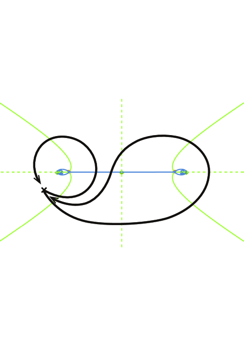
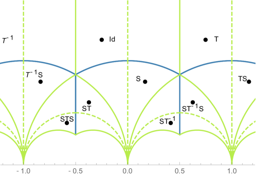
Figure 4: The upper panel: The dessin of $N_{f}=0$ SW curve ($f(u)=-\frac{1}{3}u^{2}+1$, $g(u)=-\frac{2}{27}u^{3}+\frac{1}{3}u$). The lower panel: The crossed walls and the corresponding monodromies.

The monodromy matrices for various patterns of crossings are

$$\rightarrow{\bf dG}\rightarrow{\bf G}\rightarrow = T,$$

$$\rightarrow{\bf G}\rightarrow{\bf dG}\rightarrow = T^{-1},$$

$$\rightarrow{\bf dG}\rightarrow{\bf B}\rightarrow = ~{}\rightarrow{\bf B}\rightarrow{\bf dG}\rightarrow~{}=~{}S,$$

$$\rightarrow~{}{\bf B}~{}\rightarrow{\bf G}\rightarrow = ST,$$

$$\rightarrow~{}{\bf G}~{}\rightarrow{\bf B}\rightarrow = T^{-1}S,$$ (31)

where the first wall of each row is the crossing from a shaded cell region (${\rm Im}J>0$) to an unshaded one (${\rm Im}J<0$), and the second is from an unshaded to a shaded one. The monodromy matrices are defined as

$$T=\left(\begin{array}[]{cc}1&1\\ 0&1\end{array}\right),~{}~{}~{}S=\left(\begin{array}[]{cc}0&-1\\ 1&0\end{array}\right)$$ (37)

as usual, where we say that the monodromy matrix is $\left(\begin{array}[]{cc}a&b\\ c&d\end{array}\right)$ if the modulus $\tau$ is changed to

$$\tau^{\prime}~{}=~{}M\circ\tau~{}\equiv\frac{a\tau+b}{c\tau+d}.$$ (38)

They are defined only in $PSL(2,\hbox{\mybb Z})$, i.e. up to a multiplication of $-1$.

By using the rule (31), we can immediately find the monodromy matrix for the path (30) as

$$T^{-1}S\cdot T^{-1} = T^{-1}ST^{-1}$$ (39)

$$\sim STS,$$

where $\sim$ denotes the equality in $PSL(2,\hbox{\mybb Z})$.

Similarly, the crossed walls for the right path are

$$\rightarrow{\bf G}\rightarrow{\bf dG}\rightarrow{\bf G}\rightarrow{\bf dG}\rightarrow{\bf G}\rightarrow{\bf dG}\rightarrow{\bf B}\rightarrow{\bf G}\rightarrow.$$ (40)

Using rule (31) again, we find that the monodromy is

$$T^{-1}\cdot T^{-1}\cdot T^{-1}\cdot ST = T^{-3}ST.$$ (41)

A confusing but important point of the rule is that, in the first example, the monodromy matrix $T^{-1}$ which corresponds to the crossings $\rightarrow{\bf G}\rightarrow{\bf dG}\rightarrow$ taking place after the crossings $\rightarrow{\bf G}\rightarrow{\bf B}\rightarrow$ is multiplied to $T^{-1}S$ from the right. This will be confusing because if $M=\left(\begin{array}[]{cc}a&b\\ c&d\end{array}\right)$, $M^{\prime}=\left(\begin{array}[]{cc}a^{\prime}&b^{\prime}\\ c^{\prime}&d^{\prime}\end{array}\right)$ and $\tau^{\prime}=M\circ\tau$, $\tau^{\prime\prime}=M^{\prime}\circ\tau^{\prime}$, then the monodromy matrix $M^{\prime\prime}=\left(\begin{array}[]{cc}a^{\prime\prime}&b^{\prime\prime}\\ c^{\prime\prime}&d^{\prime\prime}\end{array}\right)$ representing $\tau\mapsto\tau^{\prime\prime}=M^{\prime\prime}\circ\tau$ is given by

$$M^{\prime\prime} = M^{\prime}M,$$ (42)

in which $M^{\prime}$ is multiplied from the left.

More generally, the following statement holds: Let $\gamma$ be a path specified by the series of the walls

$$\gamma : \rightarrow{\bf W}_{1}\rightarrow{\bf W}_{2}\rightarrow\cdots\rightarrow{\bf W}_{k}\rightarrow,$$ (43)

where ${\bf W}_{i}$ $(i=1,\ldots,k)$ are either of ${\bf G}$, ${\bf B}$ or ${\bf dG}$, and let $M_{\gamma}$ denote the associated monodromy matrix of $\gamma$. $k$ is an even positive integer. (If it is odd, a shaded cell region is mapped to an unshaded cell region or vice versa, and the transformation cannot be an $SL(2,\hbox{\mybb Z})$ transformation). Let $\gamma_{1}$, $\gamma_{2}$ be paths specified by the series of the walls crossed by them

$$\gamma_{1} : \rightarrow{\bf W}^{(1)}_{1}\rightarrow{\bf W}^{(1)}_{2}\rightarrow\cdots\rightarrow{\bf W}^{(1)}_{k_{1}}\rightarrow,$$

$$\gamma_{2} : \rightarrow{\bf W}^{(2)}_{1}\rightarrow{\bf W}^{(2)}_{2}\rightarrow\cdots\rightarrow{\bf W}^{(2)}_{k_{2}}\rightarrow,$$ (44)

and let $\gamma_{1}+\!\!\!\!>\gamma_{2}$ be the jointed path

$$\gamma_{1}+\!\!\!\!>\gamma_{2} : \rightarrow{\bf W}^{(1)}_{1}\rightarrow\cdots\rightarrow{\bf W}^{(1)}_{k_{1}}\rightarrow{\bf W}^{(2)}_{1}\rightarrow\cdots\rightarrow{\bf W}^{(2)}_{k_{2}}\rightarrow,$$ (45)

where we use the new symbol $+\!\!\!\!>$ to denote the operation of jointing two paths. Then

Proposition.

$$M_{\gamma_{1}+\!\!\!>\gamma_{2}} = M_{\gamma_{1}}M_{\gamma_{2}}.$$ (46)

Remark. As we noted above, the monodromy matrix corresponding to a later crossing comes to the right, unlike (42) in which the matrix for the later transformation is multiplied from the left.

Proof. By induction with respect to the total number of crossed walls, it is enough to show the statement for the cases when $\gamma_{2}$ is any of the crossing patterns (31). Suppose that $\gamma_{1}$ starts from a cell region $C_{0}$ and ends in another $C_{1}$, and that $\gamma_{2}$ goes from the cell region $C_{1}$ to another $C_{2}$, where $\gamma_{2}$ is taken to be any of the crossing patterns (31), say, $\gamma_{2}=\rightarrow{\bf dG}\rightarrow{\bf G}\rightarrow$ and $M_{\gamma_{2}}=T$. Let $P_{\gamma_{i}}$ $(i=1,2)$ be the associated maps which send points in the cell region $C_{i-1}$ to those in the cell region $C_{i}$, respectively, such that the torus modulus over the point is $SL(2,\hbox{\mybb Z})$ equivalent. We say two points on $\hbox{\mybb P}^{1}$ are $SL(2,\hbox{\mybb Z})$ equivalent if the torus fiber moduli over them are $SL(2,\hbox{\mybb Z})$ equivalent. Using this terminology, we can say that $P_{\gamma_{i}}$ $(i=1,2)$ are the maps which send the points in $C_{i-1}$ to their $SL(2,\hbox{\mybb Z})$ equivalent points in $C_{i}$, respectively. Since $\tau(z)$ is holomorphic in $z$ and $J(\tau)$ is holomorphic in $\tau$, the domain of the map $P_{\gamma_{1}}$ is not necessarily restricted to only $C_{0}$ but can be extended to outside $C_{0}$ as far as it is in a small neighborhood of $z_{0}$.

Let $z_{0}$ be a point in $C_{0}$, and let $z_{1}=P_{\gamma_{1}}(z_{0})\in C_{1}$, $z_{2}=P_{\gamma_{2}}(z_{1})\in C_{2}$. If we denote $\tau_{i}$ $(i=0,1,2)$ be the modulus of the torus fiber over $z_{i}$ $(i=0,1,2)$, they satisfy

$$J(\tau_{i}) = \frac{4f(z_{i})^{3}}{4f(z_{i})^{3}+27g(z_{i})^{2}},$$ (47)

where $\tau_{1}$ and $\tau_{2}$ are the values analytically continued from $\tau_{0}$ along the paths $\gamma_{1}$, and then $\gamma_{2}$. Taking $\tau_{0}$ in the standard fundamental region, the transformation from $\tau_{0}$ to $\tau_{1}$ is given by $\tau_{1}~{}=~{}M_{\gamma_{1}}\circ\tau_{0}$, but consecutive transformation from $\tau_{1}$ to $\tau_{2}$ is not $M_{\gamma_{2}}\circ\tau_{1}$, as $\tau_{1}$ does not belong to the standard fundamental region in general. Rather, since $P_{\gamma_{1}}$ is locally an isomorphism between a neighborhood around $z_{0}$ and that around $z_{1}$, the final point $z_{2}$ can be written as the $P_{\gamma_{1}}$ image of $z^{\prime}_{1}$, where $z^{\prime}_{1}$ is the $SL(2,\hbox{\mybb Z})$ equivalent point in the cell region reached along the path $\gamma_{2}$ first from $z_{0}$, if $z_{2}$ is close enough to $z_{1}$ (Figure 5). If, on the other hand, $z_{2}$ is not close to $z_{1}$, we can continuously deform the complex structure of the elliptic fibration so that $z_{2}$ may come close to $z_{1}$. Since this is a continuous deformation, the monodromy transformation matrix does not change, as the entries of the matrix take discrete values. Thus we may assume that $z_{2}$ is close to $z_{1}$.

Since $\tau_{0}$ is taken in the standard fundamental region, $\tau^{\prime}_{1}$, the modulus of the torus fiber over $z^{\prime}_{1}$, is given by

$$\tau^{\prime}_{1} = M_{\gamma_{2}}\circ\tau_{0}.$$ (48)

Therefore, since $\tau_{2}=M_{\gamma_{1}}\circ\tau^{\prime}_{1}$, we find

$$\tau_{2} = M_{\gamma_{1}}\circ M_{\gamma_{2}}\circ\tau_{0}$$ (49)

$$= (M_{\gamma_{1}}M_{\gamma_{2}})\circ\tau_{0},$$

which is what the proposition claims.

In deriving (49), we did not use the fact that $\gamma_{2}$ was assumed to be a particular pattern among (31), but the relation (49) likewise holds for other pattens. This completes the proof of the proposition.

Figure 5: Taking $\tau_{0}$ in the standard fundamental region, the transformation from $\tau_{0}$ to $\tau_{1}$ is given by $\tau_{1}~{}=~{}M_{\gamma_{1}}\circ\tau_{0}$, but consecutive transformation from $\tau_{1}$ to $\tau_{2}$ is not $M_{\gamma_{2}}\circ\tau_{1}$, as $\tau_{1}$ does not belong to the standard fundamental region in general. Rather, we have $\tau_{2}=M_{\gamma_{1}}\circ\tau^{\prime}_{1}$ with $\tau^{\prime}_{1}=M_{\gamma_{2}}\circ\tau_{0}$ as $P_{\gamma_{1}}$ induces an isomorphism.

V.2 Example: Monodromies of $N_{f}=4$ $SU(2)$ Seiberg-Witten curves

The proposition (46) together with the rule (31) provides us with a very convenient method to compute the monodromy for an arbitrary Weierstrass model along an arbitrary path.

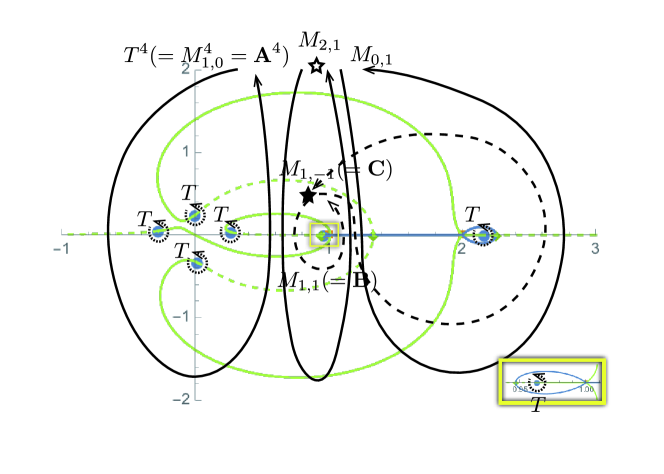
Figure 6: Monodromies of $N_{f}=4$ $SU(2)$ Seiberg-Witten curve. It shows how the monodromies around the two D-branes on the right (located at $z\approx 1$ and $\approx 2$) change depending on the choice of the reference point. If it is taken far enough (as marked as a white star), the monodromies along the black contours read $M_{2,1}$ and $M_{0,1}$. If the reference point is taken closer (as marked as a black star), then the monodromies along the dashed black contours are $M_{1,1}(={\bf B})$ and $M_{1,-1}(={\bf C})$. If, on the other hand, the reference point is taken to be very close to the D-branes inside the cell regions surrounded by the $S$-walls, then the monodromies along the dotted contours are both $T$.

Figure 6 is a dessin of $N_{f}=4$ $SU(2)$ Seiberg-Witten curve with some mass parameters. The Weierstrass equation is (1) where

$$f = (z-1)(z-2),$$

$$g = \epsilon(z-i)(z-2i)(z-3i)$$ (50)

$$+(1-\epsilon)\left(-\frac{5}{16}i\sqrt{\frac{3}{2}}z^{3}+\frac{17iz^{2}}{4\sqrt{6}}-i\sqrt{6}z+\frac{4}{3}i\sqrt{\frac{2}{3}}\right)$$

with $\epsilon=3\times 10^{-7}$. This choice of $g$ interpolates between the configuration in which all the $g$-locus planes are located on the imaginary axis at equal intervals ($\epsilon=1$) and the one in which four of the six D-branes collide together at $z=0$ to form a $I_{4}$ singular fiber ($\epsilon=0$), with the $f$-planes fixed at $z=1,2$. The figure is the configuration very close to the latter limit.

As is well known, the one-parameter (“$u$”) family of tori describe the moduli space of the gauge theory and can be compactified into a rational elliptic surface by taking the variables and coefficient functions to be sections of appropriate line bundles, where the $u$ parameter becomes the affine coordinate $z$ of the base $\hbox{\mybb P}^{1}$. Note, however, that the dessin can be drawn on this affine patch independently of the choices of the bundles; it only affects how many D-branes are at the infinity of $\hbox{\mybb P}^{1}$.

This figure shows how the monodromies around the two D-branes on the right (located at $z\approx 1$ and $\approx 2$) change depending on the choice of the reference point. If it is taken far enough (as marked as a white star), the monodromies along the black contours read $M_{2,1}$ and $M_{0,1}$. This means that, as we show later, a $(2,1)$ and a $(0,1)$ string become light near the respective D-branes, showing that the locations of the D-branes are the $(2,1)$ dyon and the monopole point on the moduli space of the gauge theory, which is well known.

If the reference point is taken closer (as marked as a black star), then the monodromies along the dashed black contours are $M_{1,1}(={\bf B})$ and $M_{1,-1}(={\bf C})$, which agrees with the ABC brane description of the $I_{0}^{*}$ Kodaira singular fiber.

Finally, if the reference point is taken to be very close to the D-branes inside the cell regions surrounded by the $S$-walls, then the monodromies along the dotted contours are both $T$, showing that these branes look ordinary D-branes if they are observed from very close to them.

V.3 $(p,q)$-brane as an effective description

Of course, it is well known that the monodromy changes depending the choice of the reference point. A monodromy matrix measured from some reference point gets $SL(2,\hbox{\mybb Z})$ conjugated if it is measured from another point. What is new here that, by drawing a dessin, we can precisely see how and from where the monodromy matrix changes and gets conjugated as we vary the position of the reference point.

For instance, we can see from Figure 6 that the monodromies around the two D-branes on the right are either $M_{2,1}$, $M_{0,1}$ or $M_{1,1}(={\bf B})$, $M_{1,-1}(={\bf C})$ for most choices of the reference point on the $z(\equiv u)$-plane, and they are recognized as ordinary ($M_{1,0}={\bf A})$ D-branes only when they are viewed from the points in the tiny regions surrounded by the $S$-walls. Thus we see that the effective description of the two branes as $(1,1)(={\bf B})$- and $(1,-1)(={\bf C})$-branes are good at the energy scale lower than the scale of the size of the small cell regions surrounded by the $S$-walls.

However, one can also set the mass parameters of the same gauge theory so that the dessin of the Seiberg-Witten curve looks as shown in Figure 1. In this case, the $S$-walls spread into wide areas of the $\hbox{\mybb P}^{1}$. There is not much difference among the six D-branes, and there is no obvious reason to distinguish particular two as B or C from the other four D-branes.

Remark. We have seen that a cluster of a D-brane and two elliptic point planes, in which the former is surrounded by the $S$-walls extended from the latter, may be effectively identified as a B- or a C-brane, if viewed from a distance of the size of the cluster. Thus one might think that an “exact” $(p,q)$-brane (whose monodromy is $M_{p,q}$ along arbitrary small loop) can be obtained by taking the $f$- and $g$-planes on top of each other so that the size of the cell region the $S$-walls surround becomes zero. This is not the case, however, since if the $f$- and $g$-planes collide, the order of the discriminant becomes two, implying that another D-brane also automatically comes on top of the D-brane, $f$-plane and $g$-plane. Since it contains two D-branes, it cannot be identified as a single $(p,q)$-brane in the ABC-brane description.

VI Conclusions

The coexistence of D-branes and non-pure-D-7-branes is an essential feature of F-theory, as it enables us to achieve exceptional group gauge symmetries or matter in spinor representations by allowing string junctions to appear as extra objects ending on more than two different types of 7-branes, in addition to the open strings which can only connect two ordinary D-branes. These 7-branes are conventionally described algebraically in terms of ABC 7-branes. In this paper, noticing that all the discriminant loci are on equal footing and there is no a priori reason to distinguish one from the others, we have considered new complex co-dimension one objects consisting of the zero loci of the coefficient functions $f$ and $g$ of the Weierstrass equation, which we referred to as an “$f$-plane” and a “$g$-plane”, collectively as “elliptic point planes”. They are two kinds of critical points of a “dessin d’enfant” known in mathematics.

Although they do not carry D-brane charges, they play an essential role in achieving an exceptional gauge symmetry and/or a spinor representation by altering the monodromies around the branes. More precisely, if there are some elliptic point planes, the $z$-plane is divided into several cell regions, each of which corresponds to a (half of a) fundamental region in the preimage of the $J$-function. A cell region is bounded by several domain walls extending from these elliptic point planes and D-branes, on which the imaginary part of the $J$-function vanishes. In particular, the elliptic point planes extend a special kind of domain walls, which we call “$S$-walls”, crossing through which implies that the type IIB complex string coupling is $S$-dualized. Consequently, on the $z$-plane coexist a theory in the perturbative regime and its nonperturbative $S$-dual simultaneously. The monodromy around several 7-branes is thus not just a product of monodromy around each 7-brane any more, but they get $SL(2,\hbox{\mybb Z})$ conjugated due to the difference of the corresponding fundamental regions the base points belong to.

In this sense one may say that the nonperturbative properties of F-theory — the realizations of exceptional group symmetry, matter in spinor representations, etc. — are the consequence of the coexisting “locally $S$-dualized regions” bounded by the $S$-walls extended from the elliptic point planes. In the orientifold limit Senorientifold , the D-branes and the elliptic point planes gather to form a $I_{0}^{*}$ singular fiber, so that the $S$-walls extended from the elliptic point planes are contracted with each other and confined, so the $S$-walls are not seen from even a short distance.

We hope this new way of presenting the non-localness among 7-branes will be useful for understanding of the structure of higher-codimension singularities with higher-rank enhancement such as discussed in MV1 ; MV2 ; BIKMSV ; HKTW ; MorrisonTaylor ; FtheoryFamilyUnification ; MizoguchiTaniAnomaly .

Appendix

Table 1: The Kodaira classification. ord$(f)$, ord$(g)$ and ord$(\Delta)$ denote the orders of zeros of $f$, $g$ and the discriminant $\Delta$ of the Weierstrass equation.

Fiber type	ord$(f)$	ord$(g)$	ord$(\Delta)$	Singularity type	7-brane configuration	Brane type
$I_{n}$	$0$	$0$	$n$	$A_{n-1}$	${\bf A}^{n}$	$A_{n-1}$
$II$	$\geq 1$	$1$	$2$	$A_{0}$	${\bf C}{\bf A}$	$H_{0}$
$III$	$1$	$\geq 2$	$3$	$A_{1}$	${\bf C}{\bf A}^{2}$	$H_{1}$
$IV$	$\geq 2$	$2$	$4$	$A_{2}$	${\bf C}{\bf A}^{3}$	$H_{2}$
$I_{n}^{*}$	$\geq 2$	$3$	$6+n$	$D_{n+4}$	${\bf A}^{n+4}{\bf B}{\bf C}$	$D_{n+4}$
$I_{n}^{*}$	$2$	$\geq 3$	$6+n$	$D_{n+4}$	${\bf A}^{n+4}{\bf B}{\bf C}$	$D_{n+4}$
$II^{*}$	$\geq 4$	$5$	$10$	$E_{8}$	${\bf A}^{7}{\bf B}{\bf C}^{2}$	$E_{8}$
$III^{*}$	$3$	$\geq 5$	$9$	$E_{7}$	${\bf A}^{6}{\bf B}{\bf C}^{2}$	$E_{7}$
$IV^{*}$	$\geq 3$	$4$	$8$	$E_{6}$	${\bf A}^{5}{\bf B}{\bf C}^{2}$	$E_{6}$

References

- (1) C. Vafa, Nucl. Phys. B 469 (1996) 403 [hep-th/9602022].
- (2) D. R. Morrison and C. Vafa, Nucl. Phys. B 473 (1996) 74 [hep-th/9602114].
- (3) D. R. Morrison and C. Vafa, Nucl. Phys. B 476 (1996) 437 [hep-th/9603161].
- (4) E. Witten, Nucl. Phys. B 471 (1996) 135 [hep-th/9602070].
- (5) R. Blumenhagen, B. Kors, D. Lust and T. Ott, Nucl. Phys. B 616 (2001) 3 [hep-th/0107138].
- (6) R. Blumenhagen, M. Cvetic, D. Lust, R. Richter and T. Weigand, Phys. Rev. Lett. 100 (2008) 061602 [arXiv:0707.1871 [hep-th]].
- (7) R. Donagi and M. Wijnholt, Adv. Theor. Math. Phys. 15, 1237 (2011) [arXiv:0802.2969 [hep-th]].
- (8) C. Beasley, J. J. Heckman and C. Vafa, JHEP 0901, 058 (2009) [arXiv:0802.3391 [hep-th]].
- (9) C. Beasley, J. J. Heckman and C. Vafa, JHEP 0901, 059 (2009) [arXiv:0806.0102 [hep-th]].
- (10) R. Donagi and M. Wijnholt, Adv. Theor. Math. Phys. 15, 1523 (2011) [arXiv:0808.2223 [hep-th]].
- (11) H. Hayashi, T. Kawano, R. Tatar and T. Watari, Nucl. Phys. B 823 (2009) 47 [arXiv:0901.4941 [hep-th]].
- (12) R. Donagi and M. Wijnholt, Commun. Math. Phys. 326 (2014) 287 [arXiv:0904.1218 [hep-th]].
- (13) J. J. Heckman, J. Marsano, N. Saulina, S. Schafer-Nameki and C. Vafa, arXiv:0808.1286 [hep-th].
- (14) J. Marsano, N. Saulina and S. Schafer-Nameki, Phys. Rev. D 80 (2009) 046006 [arXiv:0808.1571 [hep-th]].
- (15) J. J. Heckman and C. Vafa, JHEP 0909 (2009) 079 [arXiv:0809.1098 [hep-th]].
- (16) A. Font and L. E. Ibanez, JHEP 0902 (2009) 016 [arXiv:0811.2157 [hep-th]].
- (17) R. Friedman, J. Morgan and E. Witten, Commun. Math. Phys. 187 (1997) 679 [hep-th/9701162].
- (18) H. Hayashi, R. Tatar, Y. Toda, T. Watari and M. Yamazaki, Nucl. Phys. B 806 (2009) 224 [arXiv:0805.1057 [hep-th]].
- (19) B. Andreas and G. Curio, J. Geom. Phys. 60 (2010) 1089 doi:10.1016/j.geomphys.2010.03.008 [arXiv:0902.4143 [hep-th]].
- (20) J. Marsano, N. Saulina and S. Schafer-Nameki, JHEP 0908 (2009) 030 [arXiv:0904.3932 [hep-th]].
- (21) A. Collinucci, JHEP 1004 (2010) 076 [arXiv:0906.0003 [hep-th]].
- (22) R. Blumenhagen, T. W. Grimm, B. Jurke and T. Weigand, JHEP 0909 (2009) 053 [arXiv:0906.0013 [hep-th]].
- (23) J. Marsano, N. Saulina and S. Schafer-Nameki, JHEP 0908 (2009) 046 [arXiv:0906.4672 [hep-th]].
- (24) R. Blumenhagen, T. W. Grimm, B. Jurke and T. Weigand, Nucl. Phys. B 829 (2010) 325 [arXiv:0908.1784 [hep-th]].
- (25) J. Marsano, N. Saulina and S. Schafer-Nameki, JHEP 1004 (2010) 095 [arXiv:0912.0272 [hep-th]].
- (26) T. W. Grimm, S. Krause and T. Weigand, JHEP 1007 (2010) 037 [arXiv:0912.3524 [hep-th]].
- (27) M. Cvetic, I. Garcia-Etxebarria and J. Halverson, JHEP 1101 (2011) 073 [arXiv:1003.5337 [hep-th]].
- (28) C. M. Chen, J. Knapp, M. Kreuzer and C. Mayrhofer, JHEP 1010 (2010) 057 [arXiv:1005.5735 [hep-th]].
- (29) C. M. Chen and Y. C. Chung, JHEP 1103 (2011) 049 [arXiv:1005.5728 [hep-th]].
- (30) T. W. Grimm and T. Weigand, Phys. Rev. D 82 (2010) 086009 [arXiv:1006.0226 [hep-th]].
- (31) J. Knapp, M. Kreuzer, C. Mayrhofer and N. O. Walliser, JHEP 1103 (2011) 138 [arXiv:1101.4908 [hep-th]].
- (32) M. J. Dolan, J. Marsano, N. Saulina and S. Schafer-Nameki, Phys. Rev. D 84 (2011) 066008 [arXiv:1102.0290 [hep-th]].
- (33) J. Marsano and S. SchaferNameki, JHEP 1111 (2011) 098 [arXiv:1108.1794 [hep-th]].
- (34) T. W. Grimm, M. Kerstan, E. Palti and T. Weigand, JHEP 1112 (2011) 004 [arXiv:1107.3842 [hep-th]].
- (35) D. R. Morrison and D. S. Park, JHEP 1210 (2012) 128 [arXiv:1208.2695 [hep-th]].
- (36) C. Mayrhofer, E. Palti and T. Weigand, JHEP 1303 (2013) 098 [arXiv:1211.6742 [hep-th]].
- (37) V. Braun, T. W. Grimm and J. Keitel, JHEP 1309 (2013) 154 [arXiv:1302.1854 [hep-th]].
- (38) J. Borchmann, C. Mayrhofer, E. Palti and T. Weigand, Phys. Rev. D 88 (2013) no.4, 046005 [arXiv:1303.5054 [hep-th]].
- (39) M. Cvetic, D. Klevers and H. Piragua, JHEP 1306 (2013) 067 [arXiv:1303.6970 [hep-th]].
- (40) V. Braun, T. W. Grimm and J. Keitel, JHEP 1312 (2013) 069 [arXiv:1306.0577 [hep-th]].
- (41) M. Cvetic, A. Grassi, D. Klevers and H. Piragua, JHEP 1404 (2014) 010 [arXiv:1306.3987 [hep-th]].
- (42) M. Cvetič, D. Klevers and H. Piragua, JHEP 1312 (2013) 056 [arXiv:1307.6425 [hep-th]].
- (43) J. Borchmann, C. Mayrhofer, E. Palti and T. Weigand, Nucl. Phys. B 882 (2014) 1 [arXiv:1307.2902 [hep-th]].
- (44) M. Cvetic, D. Klevers, H. Piragua and P. Song, JHEP 1403 (2014) 021 [arXiv:1310.0463 [hep-th]].
- (45) I. Antoniadis and G. K. Leontaris, Phys. Lett. B 735 (2014) 226 [arXiv:1404.6720 [hep-th]].
- (46) C. Lawrie, S. Schafer-Nameki and J. M. Wong, JHEP 1509 (2015) 144 [arXiv:1504.05593 [hep-th]].
- (47) M. Cvetic, D. Klevers, H. Piragua and W. Taylor, JHEP 1511 (2015) 204 [arXiv:1507.05954 [hep-th]].
- (48) M. Cvetic, A. Grassi, D. Klevers, M. Poretschkin and P. Song, JHEP 1604 (2016) 041 [arXiv:1511.08208 [hep-th]].
- (49) Y. Kimura and S. Mizoguchi, PTEP 2018 (2018) no.4, 043B05 [arXiv:1712.08539 [hep-th]].
- (50) Y. Kimura, JHEP 1805, 048 (2018) [arXiv:1802.05195 [hep-th]].
- (51) M.R. Gaberdiel, T. Hauer and B. Zwiebach, Open string - string junction transitions, Nucl. Phys. B525 (1998) 117, hep-th/9801205.
- (52) O. DeWolfe and B. Zwiebach, String Junctions for Arbitrary Lie Algebra Represen- tations, Nucl. Phys. B541 (1999) 509, hep-th/9804210.
- (53) O. DeWolfe, T. Hauer, A. Iqbal and B. Zwiebach, Uncovering the Symmetries on [p, q] 7-branes: Beyond the Kodaira Classification, hep-th/9812028.
- (54) J. H. Schwarz, Phys. Lett. B 360 (1995) 13 Erratum: [Phys. Lett. B 364 (1995) 252] [hep-th/9508143].
- (55) T. Tani, Nucl. Phys. B 602 (2001) 434.
- (56) L. Bonora and R. Savelli, JHEP 1011 (2010) 025 [arXiv:1007.4668 [hep-th]].
- (57) M. Fukae, Y. Yamada and S-K. Yang, Nucl.Phys.B572(2000)71-94.
- (58) A. Grassi, J. Halverson and J. L. Shaneson, JHEP 1310 (2013) 205 [arXiv:1306.1832 [hep-th]].
- (59) A. Grassi, J. Halverson and J. L. Shaneson, Commun. Math. Phys. 336 (2015) no.3, 1231 [arXiv:1402.5962 [hep-th]].
- (60) A. Grothendieck, ”Esquisse d’un Programme”, (1984 manuscript). Published in Schneps and Lochak (1997, I), pp.5-48; English transl., ibid., pp. 243-283. MR1483107.
- (61) S.K.Lando and A.K.Zvonkin, ”Graphs on Surfaces and Their Applications, Encyclopaedia of Mathematical Sciences: Lower-Dimensional Topology II”, 141, (2004). Berlin, New York: Springer-Verlag, ISBN 978-3-540-00203-1, Zbl 1040.05001.
- (62) N. Seiberg and E. Witten, Nucl. Phys. B 431 (1994) 484 [hep-th/9408099].
- (63) A. Sen, Nucl. Phys. B 475 (1996) 562 [hep-th/9605150].
- (64) M. Bershadsky, K. A. Intriligator, S. Kachru, D. R. Morrison, V. Sadov and C. Vafa, Nucl. Phys. B 481 (1996) 215 [hep-th/9605200].
- (65) D. R. Morrison and W. Taylor, JHEP 1201, 022 (2012) [arXiv:1106.3563 [hep-th]].
- (66) S. Mizoguchi, JHEP 1407 (2014) 018 [arXiv:1403.7066 [hep-th]].
- (67) S. Mizoguchi and T. Tani, PTEP 2016 (2016) no.7, 073B05 [arXiv:1508.07423 [hep-th]].