Theoretical study of the direct $\alpha+d$ $\rightarrow$ ⁶Li + $\gamma$ astrophysical capture process in a three-body model II. Reaction rates and primordial abundance

Abstract

The astrophysical S-factor and reaction rate of the direct capture process $\alpha+d$ $\rightarrow$ ⁶Li + $\gamma$, as well as the abundance of the ⁶Li element are estimated in a three-body model. The initial state is factorized into the deuteron bound state and the $\alpha+d$ scattering state. The final nucleus ⁶Li(1+) is described as a three-body bound state $\alpha+n+p$ in the hyperspherical Lagrange-mesh method. Corrections to the asymptotics of the overlap integral in the S- and D-waves have been done for the E2 S-factor. The isospin forbidden E1 S-factor is calculated from the initial isosinglet states to the small isotriplet components of the final ⁶Li(1+) bound state. It is shown that the three-body model is able to reproduce the newest experimental data of the LUNA collaboration for the astrophysical S-factor and the reaction rates within the experimental error bars. The estimated ⁶Li/H abundance ratio of $(0.67\pm 0.01)\times 10^{-14}$ is in a very good agreement with the recent measurement $(0.80\pm 0.18)\times 10^{-14}$ of the LUNA collaboration.

I Introduction

There are two open astrophysical problems related to the abundance of lithium elements in the Universe. First, the Big Bang nucleosynthesis (BBN) model predicts for the ⁷Li/H ratio an estimate about three times larger than the recent astronomical observational data from metal-poor halo stars sbor10 ; Mukhamedzhanov et al. (2016). The second lithium puzzle is related to the estimation of the primordial abundance ratio ⁶Li/ ⁷Li of the lithium isotopes. For this ratio the BBN model Serpico et al. (2004) yields a value about three orders of magnitude less than the astrophysical data Asplund et al. (2006). In the BBN model the abundance of the ⁷Li element is estimated on the basis of two key capture reactions $\alpha(^{3}$He,$\gamma)^{7}$Be and $\alpha(^{3}$H,$\gamma)^{7}$Li (see neff ; navratil ; tur18 and references therein). For the estimation of the ⁶Li/⁷Li ratio the BBN model includes as input parameters the reaction rates of the direct radiative capture process

$$\alpha+d\rightarrow{\rm{}^{6}Li}+\gamma$$ (1)

at low energies within the range $30\leq E_{\rm cm}\leq 400$ keV Serpico et al. (2004). The data set of the LUNA collaboration at two astrophysical energies E=94 keV and E=134 keV Anders et al. (2014) was recently renewed with additional data at E=80 keV and E=120 keV luna17 . These data sets were obtained as results of the direct measurements of the astrophysical S-factor at the underground facility. The new data are lower than the old data of nondirect measurements from Ref. Kiener et al. (1991). Based on the new data set, the thermonuclear reaction rate of the process has been estimated by the LUNA collaboration. The results for the reaction rates turn out to be even lower than previously reported. This further increases the discrepancy between prediction of the BBN model and the astronomical observations for the primordial abundance of the ⁶Li element in the Universe luna17 .

Until recently all the theoretical estimations of the astrophysical S-factor of the above direct capture reaction at low astrophysical energies were based on the so-called exact mass prescription, in the both potential models Dubovichenko and Dzhazairov-Kakhramanov (1995a, b); Typel et al. (1997); Kharbach and Descouvemont (1998); Mukhamedzhanov et al. (2011); Tursunov et al. (2015); Mukhamedzhanov et al. (2016) and microscopic approaches Langanke (1986); Nollett et al. (2001); TBL91 . Within this prescription the matrix elements of the isospin forbidden E1-transition were estimated by using the exact experimental mass values of the colliding nuclei ²H and ⁴He. As was shown recently in Ref. bt18 in details, this way has no microscopic background at all and cannot be used, for example in the description of the capture process $d(d,\gamma)^{4}$He of two identical nuclei. Of course, the estimated in this way cross sections and S-factors of the $\alpha(d,\gamma)^{6}$Li capture reaction can be fortituously close to the experimental data, however this method does not yield a relevant energy dependence of the S-factor and cross section and correct predictive power for future $\it ab-initio$ studies bt18 . An alternative approach to the description of the capture processes is based on solving the three-body Faddeev equations shub16 using quasi-separable potentials. An advantage of this method is that it allows an easier treatment of non-local effects that can be extended to three-body problems.

Realistic three-body models are based on the isovector E1 transition from the initial $T_{i}=0$ (isosinglet) states to the $T_{f}=1$ (isotriplet) components of the final ⁶Li$(1^{+})$ bound state, or from the initial isotriplet components to the main isoscalar part of the final ⁶Li$(1^{+})$ nucleus bound state bt18 . First attempt to estimate in a correct way the matrix elements of the isospin-forbidden E1- transition together with the E2-transition for the ⁴He$(d,\gamma)^{6}$Li direct capture process has been done in the three-body model TKT16 . The formalism of the model has been developed in a consistent way and correct analytical expressions have been obtained for the matrix elements of the E1- and E2-transitions, including the isovector transition matrix elements. The numerical results were obtained on the basis of the final three-body wave function ⁶Li$=\alpha+p+n$ in hyperspherical coordinates Descouvemont et al. (2003); Tursunov et al. (2006), which had a small isotriplet component with the norm square of 1.13 $\times 10^{-5}$. Due to smallness of the isotriplet component of the final three-body bound state the corresponding numerical calculations in Ref. TKT16 have reproduced the existing experimental data for the S-factor only in the frame of the exact mass prescription and with the help of additional spectroscopic factor. Further studies in Ref. bt18 have demonstrated that the quality of the final three-body wave function ⁶Li$=\alpha+p+n$ can be improved and convergent isotriplet component can be reached with the norm square of 5.3$\times 10^{-3}$, which is larger than the old number by two orders of magnitude. This led to the fact that the E1 S-factor also increased by two orders of magnitude. Additionally, as was shown in that paper, the E2 S-factor can be improved owing to the correction of the asymptotics of the overlap integral of the ⁶Li and deuteron wave functions at a distance 5-10 fm.

The aim of present study is to estimate the reaction rates of the $\alpha(d,\gamma)^{6}$Li direct capture process and the primordial abundance of the ⁶Li element in the Universe within the improved realistic three-body model TKT16 ; bt18 . The initial wave function is factorized into the deuteron bound-state and the $\alpha-d$ scattering-state wave functions. The final ⁶Li(1+) state is described as a $\alpha+p+n$ three-body bound system. The wave function on the hyperspherical Lagrange mesh basis available for the ⁶Li(1+) bound state Descouvemont et al. (2003); Tursunov et al. (2006) will be employed.

In Sec. II we describe the model, in Sec. III we discuss obtained numerical results and finally, in the last section we draw conclusions.

II Theoretical model

II.1 Cross sections of the radiation capture process

The cross sections of the radiative capture process reads

$$\sigma_{E}(\lambda)= \sum_{J_{i}T_{i}\pi_{i}}\sum_{J_{f}T_{f}\pi_{f}}\sum_{\Omega\lambda}\frac{(2J_{f}+1)}{\left[I_{1}\right]\left[I_{2}\right]}\frac{32\pi^{2}(\lambda+1)}{\hbar\lambda\left(\left[\lambda\right]!!\right)^{2}}k_{\gamma}^{2\lambda+1}C_{s}^{2}$$

$$\times\sum_{l_{\omega}I_{\omega}}\frac{1}{k_{\omega}^{2}v_{\omega}}\mid\langle\Psi^{J_{f}T_{f}\pi_{f}}\|M_{\lambda}^{\Omega}\|\Psi_{l_{\omega}I_{\omega}}^{J_{i}T_{i}\pi_{i}}\rangle\mid^{2},$$ (2)

where $\Omega=$E or M (electric or magnetic transition), $\omega$ denotes the entrance channel, $k_{\omega}$, $v_{\omega}$, $I_{\omega}$ are the wave number, velocity of the $\alpha-d$ relative motion and the spin of the entrance channel, respectively, $J_{f}$, $T_{f}$, $\pi_{f}$ ($J_{i}$, $T_{i}$, $\pi_{i}$) are the spin, isospin and parity of the final (initial) state, $I_{1}$, $I_{2}$ are channel spins, $k_{\gamma}=E_{\gamma}/\hbar c$ is the wave number of the photon corresponding to the energy $E_{\gamma}=E_{\rm th}+E$ with the threshold energy $E_{\rm th}=1.474$ MeV. The wave functions $\Psi_{l_{\omega}I_{\omega}}^{J_{i}T_{i}\pi_{i}}$ and $\Psi^{J_{f}T_{f}\pi_{f}}$ represent the initial and final states, respectively. The reduced matrix elements are evaluated between the initial and final states. We also use short-hand notations $[I]=2I+1$ and $[\lambda]!!=(2\lambda+1)!!$.

Constant $C_{s}^{2}$ is the spectroscopic factor Angulo et al. (1999). As argued in Ref. Mukhamedzhanov et al. (2011), if the two-body potentials of the model correctly reproduce experimental phase shifts in the partial waves and physical bound state energies of the two-body subsystems, then a value of the spectroscopic factor must be taken equal to 1. This reflects the fact that the potential parameters already include many-body effects. Accordingly, the factor is set equal to 1.

The analytical expressions of the E1 and E2 electric-transition operators, including isospin transition operators and their matrix elements in the three-body model have been described in Ref. TKT16 . For the sake of brevity we refer to that paper for the details of the model.

The astrophysical $S$-factor of the process is expressed in terms of the cross section as Fowler et al. (1975)

$$S(E)=E\,\sigma_{E}(\lambda)\exp(2\pi\eta),$$ (3)

where $\eta$ is the Coulomb parameter.

II.2 Reaction rates

The reaction rate $N_{a}(\sigma v)$ is estimated according to Fowler et al. (1975); Angulo et al. (1999)

$$N_{a}(\sigma v)=N_{A}\frac{(8/\pi)^{1/2}}{\mu^{1/2}(k_{\text{B}}T)^{3/2}}\int^{\infty}_{0}\sigma(E)E\exp(-E/k_{\text{B}}T)dE,$$ (4)

where $k_{\text{B}}$ is the Boltzmann constant, $T$ is the temperature, $N_{A}=6.0221\times 10^{23}\,\text{mol}^{-1}$ is the Avogadro number. The reduced mass is written as $\mu=Am_{N}$ with the corresponding reduced mass number $A=A_{1}A_{2}/(A_{1}+A_{2})$ for the $\alpha+d$ system, where $A_{1}=2$ and $A_{2}=4$. Consequently, a value of $A=4/3$ is fixed. When a variable $k_{\text{B}}T$ is expressed in units of MeV it is convenient to use a variable $T_{9}$ for the temperature in units of $10^{9}$ K according to the equation $k_{\text{B}}T=T_{9}/11.605$ MeV. In our calculations $T_{9}$ varies in the interval $0.001\leq T_{9}\leq 10$.

After substitution of these variables the above integral for the reaction rates can be expressed as:

$$N_{a}(\sigma v) = 3.7313\times 10^{10}A^{-1/2}\,\,T_{9}^{-3/2}$$ (5)

$$\times\int^{\infty}_{0}\sigma(E)E\exp(-11.605E/T_{9})dE.$$

III Numerical results

III.1 Details of the calculations

Calculations of the cross section and astrophysical S-factor have been performed under the same conditions as in Ref.bt18 . The radial wave function of the deuteron is the solution of the bound-state Schrödinger equation with the central Minnesota potential $V_{NN}$ Thompson et al. (1977); RT70 with $\hbar^{2}/2m_{N}=20.7343$ MeV fm². The Schrödinger equation is solved using a highly accurate Lagrange-Laguerre mesh method Baye (2015). It yields $E_{d}$=-2.202 MeV for the deuteron ground-state energy with the number of mesh points $N=40$ and a scaling parameter $h_{d}=0.40$.

The scattering wave function of the $\alpha-d$ relative motion is calculated with a deep potential of Dubovichenko Dubovichenko and Dzhazairov-Kakhramanov (1994) with a small modification in the $S$-wave Tursunov et al. (2015): $V_{d}^{(S)}(R)=-92.44\exp(-0.25R^{2})$ MeV. The potential parameters in the ${}^{3}P_{0}$, ${}^{3}P_{1}$, ${}^{3}P_{2}$ and ${}^{3}D_{1}$, ${}^{3}D_{2}$, ${}^{3}D_{3}$ partial waves are the same as in Ref. Dubovichenko and Dzhazairov-Kakhramanov (1994). The potential contains additional states in the $S$- and $P$-waves forbidden by the Pauli principle. The above modification of the S-wave potential reproduces the empirical value $C_{\alpha d}=2.31$ fm^-1/2 of the asymptotic normalization coefficient (ANC) of the ⁶Li(1+) ground state derived from $\alpha-d$ elastic scattering data Blokhintsev et al. (1993).

The final ⁶Li(1+) ground-state wave function was calculated using the hyperspherical Lagrange-mesh method Descouvemont et al. (2003); Tursunov et al. (2006); tur07 with the same Minnesota NN-potential. For the $\alpha-N$ nuclear interaction the potentials of Voronchev et al. (Model A) Voronchev et al. (1995) and Kanada et al. (Model B) KKN79 were employed, which contain a deep Pauli-forbidden state in the $S$-wave. The potentials were slightly renormalized by a scaling factors 1.014 (Model A) and 1.008 (Model B) to reproduce the experimental binding energy $E_{b}$=3.70 MeV. The Coulomb interaction between $\alpha$ and proton is taken as $2e^{2}\,\mathrm{erf}(0.83\,R)/R$ RT70 . The coupled hyperradial equations are solved with the Lagrange-mesh method Baye (2015); Descouvemont et al. (2003). The hypermomentum expansion includes terms up to $K_{\rm max}=24$, which ensures a good convergence of the energy and of the $T=1$ component of ⁶Li. The ground state is essentially $S=1$ (96 %). The matter r.m.s. radius of the ground state (with 1.4 fm as $\alpha$ radius) is found as $\sqrt{r^{2}}\approx 2.25$ fm with the potential of Ref. Voronchev et al. (1995) or 2.24 fm with the potential of Ref. KKN79 , i.e. values slightly lower than the experimental value $2.32\pm 0.03$ fm Tanihata et al. (1988). The isotriplet component in the ⁶Li ground state has a squared norm $5.3\times 10^{-3}$ with the potential of Ref. Voronchev et al. (1995) (Model A) and $4.2\times 10^{-3}$ with the potential of Ref. KKN79 (Model B).

III.2 Estimation of the astrophysical S-factor

In Fig. 1 we display E1 astrophysical S-factors for the direct $\alpha+d\rightarrow^{6}$Li$+\gamma$ capture process within Model A from the initial partial ${}^{3}P_{0}$, ${}^{3}P_{1}$, ${}^{3}P_{2}$ scattering waves to the $T$=1 (isotriplet) components of the final ground state of ⁶Li.

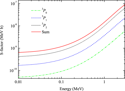
Figure 1: Partial E1 astrophysical S-factors of the direct $\alpha+d\rightarrow^{6}$Li$+\gamma$ capture process within Model A (see text).

At low astrophysical energies, the cross section is very sensitive to the asymptotic behavior of the overlap integrals of the deuteron wave function $\Psi_{d}$ and the three-body wave functions $\Psi_{f}^{1M+}$ for the $L=0$ and $L=2$ partial waves up to large $\alpha-d$ distances $R$. The asymptotic normalization coefficients (ANCs) of the ⁶Li nucleus in the $\alpha+d$ channel can be extracted within the effective range expansion method blokh17 ; blokh18 or from the analytical continuation of the scattering amplitude Blokhintsev et al. (1993).

The overlap integrals are written as

$$I_{L}(R)=\langle[\Psi_{d}\otimes Y_{L}(\Omega_{R})]^{1M}|\Psi_{f}^{1M+}\rangle,$$ (6)

where the integration is done over internal coordinates of the deuteron and the angular part of the variable $\bf{R}$. In the present three-body model, over the interval $5-10$ fm $I_{L}(R)$ follows the expected asymptotic behavior $C_{\alpha d}^{(L)}W_{-\eta_{b},L+1/2}(2k_{b}R)/R$, where $\eta_{b}$ and $k_{b}$ are the Sommerfeld parameter and wave number calculated at the separation energy 1.474 MeV of the ⁶Li bound state into $\alpha$ and $d$ bt18 . The values of the S-wave and D-wave asymptotic normalization coefficients (ANC) have been estimated for different values of matching point $R_{0}$. We found that S-wave ANC is maximal (consequently optimal) for the matching point at 5.5 fm: $C_{\alpha d}^{(0)}=2.116$ fm^-1/2 and $C_{\alpha d}^{(0)}=2.051$ fm^-1/2 for Model A and Model B, respectively. The first number is slightly larger than $C_{\alpha d}^{(0)}\approx 2.05$ fm^-1/2 bt18 , obtained with $R_{0}=7.75$ fm and in reasonable agreement with the value $C_{\alpha d}^{(0)}\approx 2.30$ fm^-1/2 extracted in Ref. Blokhintsev et al. (1993) from experimental data on $\alpha+d$ scattering. The estimated values of D-wave ANC are less than the corresponding values of the S-wave ANC by two orders of magnitude and vary in the range between $2.160\times 10^{-2}$ and $2.175\times 10^{-2}$ fm^-1/2 for model A for matching points from $R_{0}=$5.5 fm to 7.5 fm. Model B yields the range between $2.179\times 10^{-2}$ and $2.188\times 10^{-2}$ fm^-1/2, respectively.

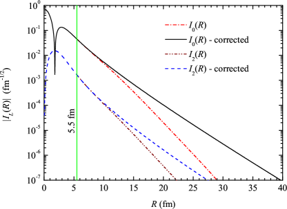
Figure 2: Overlap integral with the initial three-body and the corrected (at $R_{0}$=5.5 fm) asymptotics within Model A.

In Fig. 2 the overlap integrals $I_{0}(r)$ and $I_{2}(r)$ with the initial three-body and the asymptotics corrected at $R_{0}=5.5$ fm, within Model A are displayed. The S-wave overlap integral changes the sign at small distances due to orthogonality to the $\alpha-d$ Pauli-forbidden state, this is why the absolute values of the overlap integrals are shown. As can be seen from the figure, beyond about 10 fm the absolute value of $I_{L}(R)$ decreases faster than the correct asymptotics. Hence, within the three-body model, the E2 astrophysical S-factor is underestimated at low collision energies. This is the motivation to estimate the E2 S-factor with corrected asymptotics of the overlap integral.

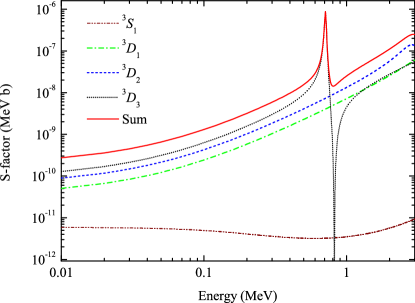
Figure 3: Partial E2 astrophysical S-factors of the direct $\alpha+d\rightarrow^{6}$Li$+\gamma$ capture process within Model A with the corrected asymptotics of the overlap integral.

In Fig. 3 we show E2 astrophysical S-factors for the direct $\alpha+d\rightarrow^{6}$Li$+\gamma$ capture process within Model A from the initial ${}^{3}S_{1}$, ${}^{3}D_{1}$, ${}^{3}D_{2}$, ${}^{3}D_{3}$ partial waves to the ground state of ⁶Li with the corrected asymptotics of $I_{0}(R)$ and $I_{2}(R)$ at a distance $R_{0}=5.5$ fm. As can be seen from the figure, at low energies the contribution of the partial ${}^{3}S_{1}$ $\alpha+d$ configuration is less than the contributions of partial D-waves at least by an order of magnitude. However, the S-wave contribution has a weak energy dependence, while the smallest ${}^{3}D_{1}$ wave contribution increases sharply from $5\times 10^{-11}$ up to $6\times 10^{-8}$ MeV b within the same energy interval.

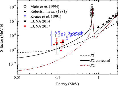
Figure 4: Relative contributions of the E1 and E2 astrophysical S-factors of the direct $\alpha+d\rightarrow^{6}$Li$+\gamma$ capture process within Model A in comparison with available experimental data.

In Fig. 4 we compare the E1 and E2 transition components of the S-factor with available experimental data, including recent data from Refs. Anders et al. (2014); luna17 . As can be seen from the figure, at low energies the E1 transition dominates even with corrected asymptotics of the overlap integral for the E2 transition, while at higher energies the E2 component is stronger. Finally, in Fig. 5 we compare the obtained theoretical results for the astrophysical S-factor of the direct $\alpha+d\rightarrow^{6}$Li$+\gamma$ capture process with experimental data from Refs. Mohr et al. (1994); Robertson et al. (1981); Kiener et al. (1991); Anders et al. (2014); luna17 . One can note that Figs. 4 and 5 are very similar to Figs. 1 and 2 of Ref. bt18 , respectively. In fact, presently we include also a correction to the D-wave asymptotics of the overlap integral. Indeed, due to small values of the D-wave ANC of order 10^-2, the corresponding E2 S-factor is very small and one can not see its difference from the results of Ref. bt18 . However, even small D-wave corrections can give a non-negligible contribution to the reaction rates of the process.

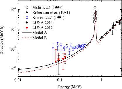
Figure 5: Theoretical astrophysical S-factor for the direct $\alpha+d\rightarrow^{6}$Li$+\gamma$ capture process within Models A and B in comparison with available experimental data.

As was noted in Ref. bt18 , the E2 S-factor can be enhanced owing to the D-wave components of the deuteron, ⁴He and the final ⁶Li nucleus with the help of tensor forces in microscopic $\it ab-initio$ models. Together with the aforementioned weak dependence of the E2 S-factor from the initial S-wave at very low energies this can lead to a larger S-wave contribution for the process at low astrophysical energies.

III.3 Reaction rates and abundance

In Table 1 we give theoretical estimations for the $d(\alpha,\gamma)^{6}$Li reaction rates in the temperature interval $10^{6}$ K $\leq T\leq 10^{10}$ K ($0.001\leq T_{9}\leq 10$) calculated with the two $\alpha+N$ potentials of Voronchev et al. Voronchev et al. (1995) (Model A) and Kanada et al KKN79 (Model B). In the second and third columns of the table we give ”the most effective energy” $E_{0}$ and the width of the Gamov window $\Delta E_{0}$ (5). They are expressed as Angulo et al. (1999):

$$E_{0} = \left(\frac{\mu}{2}\right)^{1/3}\left(\frac{\pi e^{2}Z_{1}Z_{2}k_{B}T}{\hbar}\right)^{2/3}$$ (7)

$$= 0.122\,(Z_{1}^{2}Z_{2}^{2}A)^{1/3}T_{9}^{2/3}\,[\textrm{MeV}],$$

and

$$\Delta E_{0} = 4\left(E_{0}k_{B}T/3\right)^{1/2}$$ (8)

$$= 0.2368\,(Z_{1}^{2}Z_{2}^{2}A)^{1/6}T_{9}^{5/6}\,[\textrm{MeV}].$$

Table 1: Theoretical estimations of the direct ${d}(\alpha,\gamma)^{6}{\rm Li}$ capture reaction rate in the temperature interval $10^{6}$ K $\leq T\leq 10^{10}$ K ($0.001\leq T_{9}\leq 10$).

$T_{9}$	$E_{0}$ (MeV)	$\Delta E_{0}$ (MeV)	$N_{a}(\sigma v)$ ($\textrm{cm}^{3}\rm{mol}^{-1}\rm{s}^{-1}$)			$T_{9}$	$E_{0}$ (MeV)	$\Delta E_{0}$ (MeV)	$N_{a}(\sigma v)$ ($\textrm{cm}^{3}\rm{mol}^{-1}\rm{s}^{-1}$)
			Model A	Model B					Model A	Model B
0.001	0.002	0.001	$3.47\times 10^{-30}$	$2.37\times 10^{-30}$		0.120	0.052	0.054	$1.83\times 10^{-5}$	$1.38\times 10^{-5}$
0.002	0.003	0.002	$1.04\times 10^{-23}$	$7.14\times 10^{-24}$		0.130	0.055	0.057	$2.68\times 10^{-5}$	$2.03\times 10^{-5}$
0.003	0.004	0.003	$1.42\times 10^{-20}$	$9.74\times 10^{-21}$		0.140	0.058	0.061	$3.79\times 10^{-5}$	$2.88\times 10^{-5}$
0.004	0.005	0.003	$1.33\times 10^{-18}$	$9.18\times 10^{-19}$		0.150	0.060	0.064	$5.21\times 10^{-5}$	$3.96\times 10^{-5}$
0.005	0.006	0.004	$3.36\times 10^{-17}$	$2.32\times 10^{-17}$		0.160	0.063	0.068	$6.96\times 10^{-5}$	$5.31\times 10^{-5}$
0.006	0.007	0.004	$3.93\times 10^{-16}$	$2.72\times 10^{-16}$		0.180	0.068	0.075	$1.17\times 10^{-4}$	$8.96\times 10^{-5}$
0.007	0.008	0.005	$2.79\times 10^{-15}$	$1.93\times 10^{-15}$		0.200	0.073	0.082	$1.83\times 10^{-4}$	$1.41\times 10^{-4}$
0.008	0.009	0.006	$1.41\times 10^{-14}$	$9.77\times 10^{-15}$		0.250	0.085	0.099	$4.53\times 10^{-4}$	$3.54\times 10^{-4}$
0.009	0.009	0.006	$5.52\times 10^{-14}$	$3.83\times 10^{-14}$		0.300	0.096	0.115	$9.17\times 10^{-4}$	$7.23\times 10^{-4}$
0.010	0.010	0.007	$1.79\times 10^{-13}$	$1.25\times 10^{-13}$		0.350	0.106	0.131	$1.62\times 10^{-3}$	$1.29\times 10^{-3}$
0.011	0.011	0.007	$5.00\times 10^{-13}$	$3.48\times 10^{-13}$		0.400	0.116	0.146	$2.62\times 10^{-3}$	$2.10\times 10^{-3}$
0.012	0.011	0.008	$1.24\times 10^{-12}$	$8.66\times 10^{-13}$		0.500	0.134	0.176	$5.68\times 10^{-3}$	$4.60\times 10^{-3}$
0.013	0.012	0.008	$2.80\times 10^{-12}$	$1.96\times 10^{-12}$		0.600	0.152	0.205	$1.06\times 10^{-2}$	$8.67\times 10^{-3}$
0.014	0.012	0.009	$5.82\times 10^{-12}$	$4.08\times 10^{-12}$		0.700	0.168	0.233	$1.79\times 10^{-2}$	$1.49\times 10^{-2}$
0.015	0.013	0.010	$1.13\times 10^{-11}$	$7.94\times 10^{-12}$		0.800	0.184	0.260	$2.88\times 10^{-2}$	$2.43\times 10^{-2}$
0.016	0.014	0.010	$2.08\times 10^{-11}$	$1.46\times 10^{-11}$		0.900	0.199	0.287	$4.43\times 10^{-2}$	$3.80\times 10^{-2}$
0.018	0.015	0.011	$6.11\times 10^{-11}$	$4.30\times 10^{-11}$		1.000	0.213	0.313	$6.56\times 10^{-2}$	$5.70\times 10^{-2}$
0.020	0.016	0.012	$1.55\times 10^{-10}$	$1.09\times 10^{-10}$		1.500	0.279	0.439	$2.72\times 10^{-1}$	$2.45\times 10^{-1}$
0.025	0.018	0.015	$9.90\times 10^{-10}$	$7.03\times 10^{-10}$		2.000	0.338	0.558	$6.04\times 10^{-1}$	$5.50\times 10^{-1}$
0.030	0.021	0.017	$4.08\times 10^{-9}$	$2.91\times 10^{-9}$		2.500	0.393	0.672	$9.88\times 10^{-1}$	$8.99\times 10^{-1}$
0.040	0.025	0.021	$3.23\times 10^{-8}$	$2.32\times 10^{-8}$		3.000	0.443	0.782	$1.39$	$1.26$
0.050	0.029	0.026	$1.41\times 10^{-7}$	$1.02\times 10^{-7}$		4.000	0.537	0.994	$2.26$	$2.02$
0.060	0.033	0.030	$4.35\times 10^{-7}$	$3.18\times 10^{-7}$		5.000	0.623	1.197	$3.24$	$2.87$
0.070	0.036	0.034	$1.07\times 10^{-6}$	$7.88\times 10^{-7}$		6.000	0.704	1.393	$4.35$	$3.83$
0.080	0.040	0.038	$2.26\times 10^{-6}$	$1.67\times 10^{-6}$		7.000	0.780	1.584	$5.54$	$4.87$
0.090	0.043	0.042	$4.27\times 10^{-6}$	$3.17\times 10^{-6}$		8.000	0.853	1.771	$6.78$	$5.95$
0.100	0.046	0.046	$7.38\times 10^{-6}$	$5.51\times 10^{-6}$		9.000	0.922	1.953	$8.05$	$7.06$
0.110	0.049	0.050	$1.19\times 10^{-5}$	$8.94\times 10^{-6}$		10.00	0.989	2.133	$9.31$	$8.16$

Table 2: The fitting coefficients of the analytical approximation for the direct ${d}(\alpha,\gamma)^{6}{\rm Li}$ capture reaction rate.

Model	$p_{0}$	$p_{1}$	$p_{2}$	$p_{3}$	$p_{4}$	$p_{5}$	$p_{6}$	$p_{7}$	$p_{8}$
A	6.004	-2.558	34.730	-115.482	205.801	-169.456	71.428	-11.614	42.354
B	5.154	-5.830	52.356	-163.500	272.839	-218.444	89.174	-14.107	41.384

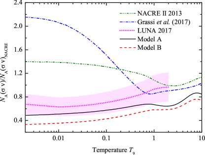
Figure 6: Reaction rates of the direct $\alpha+d\rightarrow^{6}$Li$+\gamma$ capture process within Models A and B normalized to the NACRE 1999 experimental data.

In Fig. 6 we display the estimated reaction rates of the direct $\alpha+d\rightarrow^{6}$Li$+\gamma$ capture process within Models A and B normalized to the standard NACRE 1999 experimental data NACRE99 . For comparison we also display the lines corresponding to the adopted values of the NACRE II 2013 data NACRE13 , new LUNA 2017 LUNA17 data and data fit from Ref. Laura17 . As can be seen from the figure, our results obtained within Models A and B show the same temperature dependence at low values of $T_{9}$, as the newest direct data of the LUNA 2017 LUNA17 and differs from the data NACRE II 2013 NACRE13 and the data fit in Ref. Laura17 . Consequently, the corresponding energy dependence of the astrophysical S-factor, obtained in the developed theoretical model is mostly consistent with the last direct data of the LUNA collaboration LUNA17 .

For the estimation of the abundance of the ⁶Li element, the theoretical reaction rate is approximated within 1.84% (Model A) and 2.46 % (Model B) using the following analytical formula:

$$N_{24}(\sigma v) = p_{0}T_{9}^{-2/3}\exp(-7.423T_{9}^{-1/3})$$ (9)

$$\times\left[1+p_{1}T_{9}^{1/3}+p_{2}T_{9}^{2/3}+p_{3}T_{9}+p_{4}T_{9}^{4/3}\right.$$

$$+\left.p_{5}T_{9}^{5/3}+p_{6}T_{9}^{2}+p_{7}T_{9}^{7/3}\right]$$

$$+p_{8}T_{9}^{-3/2}\exp(-7.889T_{9}^{-1}).$$

The coefficients of the analytical polynomial approximation of the $d(\alpha,\gamma)^{6}$Li reaction rates estimated with the $\alpha+N$ potential of Voronchev et al. (Model A) and Kanada et al. (Model B) are given in Table 2 in the temperature interval ($0.001\leq T_{9}\leq 10$).

On the basis of the theoretical reaction rates and with the help of the PArthENoPE Pisanti08 public code we have estimated the primordial abundance of the ⁶Li element. If we adopt the Planck 2015 best fit for the baryon density parameter $\Omega_{b}h^{2}=0.02229^{+0.00029}_{-0.00027}$ ade16 and the neutron life time $\tau_{n}=880.3\pm 1.1$ s olive14 , for the ⁶Li/H abundance ratio we have an estimation from $0.66\times 10^{-14}$ to $0.68\times 10^{-14}$ within Model A. Model B yields an estimation from $0.49\times 10^{-14}$ to $0.51\times 10^{-14}$. The results of Model A are mostly consistent with the new estimation ⁶Li/H=$(0.80\pm 0.18)\times 10^{-14}$ of the LUNA collaboration LUNA17 than the models based on the exact mass prescription method Laura17 ⁶Li/H=$(0.90-1.8)\times 10^{-14}$. Finally, using this result and the estimate of the ⁷Li/H abundance ratio of $(5.2\pm 0.4)\times 10^{-10}$ from Ref. kontos13 we get ⁶Li/⁷Li=$(1.30\pm 0.12)\times 10^{-5}$ which agrees with the standard estimate from the BBN model Serpico et al. (2004).

IV Conclusions

The astrophysical direct capture process $\alpha+d\rightarrow^{6}$Li$+\gamma$ has been studied in the three-body model. The reaction rates, E1 and E2 astrophysical S-factors as well as the primordial abundance of the ⁶Li element have been estimated. The asymptotics of the overlap integral in the S- and D-waves have been corrected. This increased the E2 S-factor by an order of magnitude at low astrophysical energies. Together with the corrected E2 S-factor, the contribution of the E1-transition operator to the S-factor from the initial isosinglet states to the small isotriplet components of the final ⁶Li(1+) bound state is shown to be able to reproduce the new experimental data of the LUNA collaboration within the experimental error bars. The theoretical reaction rates have the same temperature dependence at low temperatures as the newest direct 2017 data of the LUNA collaboration. For the abundance ratio ⁶Li/H we have obtained an estimation $(0.67\pm 0.01)\times 10^{-14}$ , consistent with the new estimation of the LUNA collaboration and much lower than the results of the models based on the exact mass prescription. Further improvement of the theoretical estimations of the reaction rates and ⁶Li abundance is expected with the help of NN-tensor forces within ab-initio calculations.

- (1) L. Sbordone, P. Bonifacio, E. Caffau et al., Astron. Astrophys. 522, A26 (2010).
- Mukhamedzhanov et al. (2016) A. M. Mukhamedzhanov, Shubhchintak, and C. A. Bertulani, Phys. Rev. C 93, 045805 (2016).
- Serpico et al. (2004) P. D. Serpico, S. Esposito, F. Iocco, G. Mangano, G. Miele, and O. Pisanti, J. Cosmol. Astropart. Phys. 2004, 010 (2004).
- Asplund et al. (2006) M. Asplund, D. L. Lambert, P. E. Nissen, F. Primas, and V. V. Smith, Astrophys. J. 644, 229 (2006).
- Anders et al. (2014) M. Anders, D. Trezzi, R. Menegazzo, M. Aliotta, A. Bellini, D. Bemmerer, C. Broggini, A. Caciolli, P. Corvisiero, H. Costantini, T. Davinson, Z. Elekes, M. Erhard, A. Formicola, Z. Fülöp, G. Gervino, A. Guglielmetti, C. Gustavino, G. Gyürky, M. Junker, A. Lemut, M. Marta, C. Mazzocchi, P. Prati, C. Rossi Alvarez, D. A. Scott, E. Somorjai, O. Straniero, and T. Szücs (LUNA Collaboration), Phys. Rev. Lett. 113, 042501 (2014).
- (6) D. Trezzi, M. Anders, M. Aliotta et al. Astropart. Phys. 89 57 (2017).
- (7) T. Neff, Phys. Rev. Lett. 106 042502 (2011).
- (8) J. Dohet-Eraly, P. Navratil, S. Quaglioni, W. Horiuchi, G. Hupin, and F. Raimondi, Phys. Lett. B 757 430 (2016).
- (9) E. M. Tursunov, S. A. Turakulov, A. S. Kadyrov, Phys. Rev. C 97 035802 (2018).
- Kiener et al. (1991) J. Kiener, H. J. Gils, H. Rebel, S. Zagromski, G. Gsottschneider, N. Heide, H. Jelitto, J. Wentz, and G. Baur, Phys. Rev. C 44, 2195 (1991).
- Dubovichenko and Dzhazairov-Kakhramanov (1995a) S. B. Dubovichenko and A. V. Dzhazairov-Kakhramanov, Phys. At. Nucl. 58, 579 (1995a).
- Dubovichenko and Dzhazairov-Kakhramanov (1995b) S. B. Dubovichenko and A. V. Dzhazairov-Kakhramanov, Phys. At. Nucl. 58, 788 (1995b).
- Typel et al. (1997) S. Typel, H. Wolter, and G. Baur, Nucl. Phys. A 613, 147 (1997).
- Kharbach and Descouvemont (1998) A. Kharbach and P. Descouvemont, Phys. Rev. C 58, 1066 (1998).
- Mukhamedzhanov et al. (2011) A. M. Mukhamedzhanov, L. D. Blokhintsev, and B. F. Irgaziev, Phys. Rev. C 83, 055805 (2011).
- Tursunov et al. (2015) E. M. Tursunov, S. A. Turakulov, and P. Descouvemont, Phys. At. Nucl. 78, 193 (2015).
- Langanke (1986) K. Langanke, Nucl. Phys. A 457, 351 (1986).
- Nollett et al. (2001) K. M. Nollett, R. B. Wiringa, and R. Schiavilla, Phys. Rev. C 63, 024003 (2001).
- (19) S. Typel, G. Blüge, and K. Langanke, Z. Phys. A 339 335 (1991).
- (20) D. Baye and E. M. Tursunov, J. Phys. G: Nucl. Part. Phys. 45 085102 (2018).
- (21) E. M. Tursunov, A. S. Kadyrov, S. A. Turakulov and I. Bray, Phys. Rev. C 94 015801 (2016).
- Descouvemont et al. (2003) P. Descouvemont, C. Daniel, and D. Baye, Phys. Rev. C 67, 044309 (2003).
- Tursunov et al. (2006) E. M. Tursunov, D. Baye, and P. Descouvemont, Phys. Rev. C 73, 014303 (2006).
- (24) Shubhchintak, C A Bertulani, A M Mukhamedzhanov and A T Kruppa, J. Phys. G: Nucl. Part. Phys. 43 125203 (2016).
- Angulo et al. (1999) C. Angulo, M. Arnould, M. Rayet, P. Descouvemont, D. Baye, C. Leclercq-Willain, A. Coc, S. Barhoumi, P. Aguer, C. Rolfs, R. Kunz, J. Hammer, A. Mayer, T. Paradellis, S. Kossionides, C. Chronidou, K. Spyrou, S. Degl’Innocenti, G. Fiorentini, B. Ricci, S. Zavatarelli, C. Providencia, H. Wolters, J. Soares, C. Grama, J. Rahighi, A. Shotter, and M. L. Rachti, Nucl. Phys. A 656, 3 (1999).
- Fowler et al. (1975) W. A. Fowler, G. R. Caughlan, and B. A. Zimmerman, Annu. Rev. Astron. Astrophys. 13, 69 (1975).
- Thompson et al. (1977) D. Thompson, M. Lemere, and Y. Tang, Nucl. Phys. A 286, 53 (1977).
- (28) I. Reichstein and Y. C. Tang, Nucl. Phys. A 158 529 (1970).
- Baye (2015) D. Baye, Phys. Rep. 565, 1 (2015).
- Dubovichenko and Dzhazairov-Kakhramanov (1994) S. B. Dubovichenko and A. V. Dzhazairov-Kakhramanov, Phys. At. Nucl. 57, 733 (1994).
- Blokhintsev et al. (1993) L. D. Blokhintsev, V. I. Kukulin, A. A. Sakharuk, D. A. Savin, and E. V. Kuznetsova, Phys. Rev. C 48, 2390 (1993).
- (32) E. M. Tursunov, P. Descouvemont and D. Baye, Nucl. Phys. A 793 52 (2007).
- Voronchev et al. (1995) V. Voronchev, V. Kukulin, V. Pomerantsev, and G. Ryzhikh, Few-Body Syst. 18, 191 (1995).
- (34) H. Kanada, T. Kaneko, S. Nagata and M. Nomoto, Prog. Theor. Phys. 61 1327 (1979).
- Tanihata et al. (1988) I. Tanihata, T. Kobayashi, O. Yamakawa, S. Shimoura, K. Ekuni, K. Sugimoto, N. Takahashi, T. Shimoda, and H. Sato, Phys. Lett. B 206, 592 (1988).
- (36) L. D. Blokhintsev, A. S. Kadyrov, A. M. Mukhamedzhanov, and D. A. Savin, Phys. Rev. C 95, 044618 (2017).
- (37) L. D. Blokhintsev, A. S. Kadyrov, A. M. Mukhamedzhanov, and D. A. Savin, Phys. Rev. C 97, 024602 (2018).
- Mohr et al. (1994) P. Mohr, V. Kölle, S. Wilmes, U. Atzrott, G. Staudt, J. W. Hammer, H. Krauss, and H. Oberhummer, Phys. Rev. C 50, 1543 (1994).
- Robertson et al. (1981) R. G. H. Robertson, P. Dyer, R. A. Warner, R. C. Melin, T. J. Bowles, A. B. McDonald, G. C. Ball, W. G. Davies, and E. D. Earle, Phys. Rev. Lett. 47, 1867 (1981).
- (40) C. Angulo et al. (NACRE), Nucl. Phys. A 656 3 (1999).
- (41) Y. Xu, K. Takahashi, S. Gorielya, M. Arnould, M. Ohtac, H. Utsunomiya (NACRE II). Nucl. Phys. A 918 61 (2013).
- (42) D. Trezzi, M. Anders, M. Aliotta et al. (LUNA collaboration), Astropart. Phys. 89 57 (2017).
- (43) A. Grassi, G. Mangano, L.E. Marcucci and O. Pisanti, Phys. Rev. C 96 045807 (2017).
- (44) O. Pisanti, A. Cirillo, S. Esposito, F. Iocco, G. Mangano, G. Miele, and P. D. Serpico, Comput. Phys. Commun. 178 956 (2008).
- (45) P. A. R. Ade et al. (Planck Collaboration), Astron. Astrophys. 594 A13 (2016).
- (46) K. A. Olive, K. Agashe, C. Amsler et al., Chin. Phys. C, 38 090001 (2014).
- (47) A. Kontos, E. Uberseder, R. deBoer, J. Görres, C. Akers, A. Best, M. Couder, M. Wiescher, Phys. Rev. C 87 (2013) 065804 (2013).