Anapole Dark Matter after DAMA/LIBRA-phase2

Abstract

We re–examine the case of anapole dark matter as an explanation for the DAMA annual modulation in light of the DAMA/LIBRA–phase2 results and improved upper limits from other DM searches. If the WIMP velocity distribution is assumed to be a Maxwellian, anapole dark matter is unable to provide an explanation of the DAMA modulation compatible with the other searches. Nevertheless, anapole dark matter provides a better fit to the DAMA–phase2 modulation data than an isoscalar spin–independent interaction, due to its magnetic coupling with sodium targets. A halo-independent analysis shows that explaining the DAMA modulation above 2 keVee in terms of anapole dark matter is basically impossible in face of the other null results, while the DAMA/LIBRA–phase2 modulation measurements below 2 keVee are marginally allowed. We conclude that in light of current measurements, anapole dark matter does not seem to be a viable explanation for the totality of the DAMA modulation.

1 Introduction

Weakly Interacting Massive Particles (WIMPs) provide one of the most popular explanations for the Dark Matter (DM) that is believed to make up 27% of the total mass density of the Universe [1] and more than 90% of the halo of our Galaxy. The scattering rate of DM WIMPs in a terrestrial detector is expected to present a modulation with a period of one year due to the Earth revolution around the Sun [2]. For more than 15 years, the DAMA collaboration [3, 4, 5] has been measuring a yearly modulation effect in their sodium iodide target. The DAMA annual modulation is consistent with what is expected from DM WIMPs, and has a statistical significance of more than $9\sigma$. However, in the most popular WIMP scenarios used to explain the DAMA signal as due to DM WIMPs, the DAMA modulation appears incompatible with the results from many other DM experiments that have failed to observe any signal so far.

This has prompted the need to extend the class of WIMP models. In particular, one of the few phenomenological scenarios that have been shown [6] to explain the DAMA effect in agreement with the constraints from other experiments is Anapole Dark Matter (ADM) [7, 8, 9, 10], for WIMP masses $m_{\chi}\mathrel{\mathop{\kern 0.0pt\hbox to0.0pt{\raise 0.86108pt\hbox{$<$}\hss}}\lower 3.87495pt\hbox{\kern-1.90002pt$\sim$}}$ 10 GeV/c².

Recently the DAMA collaboration has released first results from the upgraded DAMA/ LIBRA-phase2 experiment [11], increasing the significance of the effect to 12 $\sigma$. The two most important improvements compared to the previous phases are that now the exposure has almost doubled and the energy threshold has been lowered from 2 keV electron–equivalent (keVee) to 1 keVee. While for $m_{\chi}\mathrel{\mathop{\kern 0.0pt\hbox to0.0pt{\raise 0.86108pt\hbox{$<$}\hss}}\lower 3.87495pt\hbox{\kern-1.90002pt$\sim$}}10$ GeV/c² the DAMA phase–1 data where only sensitive to WIMP–sodium scattering events, the new data below 2 keVee are in principle also sensitive to WIMP-iodine scattering, for WIMP speeds below the escape velocity in our Galaxy. This feature has worsened the goodness of fit of the DAMA data using a standard Spin-Independent interaction (SI) [12, 13].

In light of the DAMA/LIBRA–phase2 result, in the present paper we re–examine the ADM scenario. Moreover, compared to the analyses in [6], we upgrade the constraints from other direct detection experiments. In this analysis we use results from CDEX [14], CDMSlite [15], COUPP [16], CRESST-II [17, 18], DAMIC [19], DarkSide–50  [20], KIMS [21], PANDAX-II [22], PICASSO [23], PICO-60 [24, 25], SuperCDMS [26] and XENON1T [27, 28].

The paper is organized as follows. In Section 2 we summarize the main features of the ADM scenario, providing the formulas for WIMP direct detection expected rates; our main results are in Section 3, where we provide an updated assessment of ADM in light of the DAMA–phase2 data and of the latest constraints from other direct detection experiments, both assuming a Maxwellian WIMP velocity distribution and in a halo–independent approach. Section 4 is devoted to our conclusions. In Appendix A we provide some details on how the experimental constraints on ADM have been obtained.

2 The model

Anapole dark matter (ADM) is a spin–1/2 Majorana particle that interacts with ordinary matter through the exchange of a standard photon. The ADM–photon interaction Lagrangian density is

$${\cal L}=\frac{1}{2}\frac{g}{\Lambda^{2}}\,\bar{\chi}\gamma^{\mu}\gamma^{5}\chi\,\partial^{\nu}F_{\mu\nu},$$ (2.1)

where $\chi$ is the ADM field, $F_{\mu\nu}$ is the electromagnetic field strength tensor, $g$ is a dimensionless coupling constant, and $\Lambda$ is a new physics scale.

In the nonrelativistic limit, the Hamiltonian for an ADM particle in an electromagnetic field reduces to a coupling between the WIMP spin operator $\vec{S}_{\chi}$ and the curl of the magnetic field $\vec{B}$, which by Maxwell’s equations is proportional to the electromagnetic current density, $H=-(2g/\Lambda^{2})\,\vec{S}_{\chi}\cdot\vec{\nabla}\times\vec{B}$.

The nonrelativistic scattering of an ADM particle with a nucleon can also be described by the contact interaction Hamiltonian

$$H_{\chi N}=\frac{2eg}{\Lambda^{2}}\,\vec{S}^{\perp}_{\chi}\cdot\bigg{(}e_{N}\vec{v}_{\chi N}^{\perp}+i\frac{g_{N}}{2m_{N}}\,\vec{q}\cdot\vec{S}_{N}\bigg{)}.$$ (2.2)

Here $e$ is the elementary charge, $e_{N}$ is the nucleon charge in units of $e$ ($e_{\rm p}=1$, $e_{\rm n}=0$), $g_{N}$ is the nucleon magnetic moment in units of nuclear magnetons $e/2m_{N}$ ($g_{\rm p}=5.585\,694\,713(46)$, $g_{\rm n}=-3.826\,085\,45(90)$), $m_{N}$ is the nucleon mass, $\vec{S}_{\chi}$ and $\vec{S}_{N}$ are the spins of the WIMP and the nucleon, respectively, $\vec{q}$ is the momentum transfer, and $\vec{v}^{\perp}_{\chi N}$ is the component of the WIMP–nucleon relative velocity perpendicular to $\vec{q}$.

The differential cross section per unit nucleus recoil energy $E_{R}$ for the scattering of an ADM particle of speed $v$ off a nucleus $T$ of mass $m_{T}$ at rest is given by [6]

$$\frac{\text{d}\sigma_{T}}{\text{d}E_{\text{R}}}=\sigma_{\rm ref}\frac{m_{T}}{m_{\chi N}^{2}}\frac{v_{\rm min}^{2}}{v^{2}}\left[Z_{T}^{2}\left(\frac{v^{2}}{v_{\rm min}^{2}}-1\right)F_{{\rm E},T}^{2}(q^{2})+2\mu_{T}^{2}\frac{m_{\chi T}^{2}}{m_{N}^{2}}\left(\frac{J_{T}+1}{3J_{T}}\right)F_{{\rm M},T}^{2}(q^{2})\right].$$ (2.3)

Here $v_{\rm min}$ is the minimum WIMP speed necessary to transfer energy $E_{R}$, $q^{2}=2m_{T}E_{\text{R}}$ is the square of the momentum transfer, $m_{\chi N}$ and $m_{\chi T}$ are the DM–nucleon and DM–nucleus reduced masses, respectively, $Z_{T}$ is the atomic number of the nucleus, $\mu_{T}$ is the magnetic moment of the nucleus in units of the nuclear magneton $e/2m_{N}$, $J_{T}$ is the nucleus spin, and we have defined a reference cross section

$$\sigma_{\rm ref}\equiv\frac{2m_{\chi N}^{2}\,\alpha g^{2}}{\Lambda^{4}}\,,$$ (2.4)

where $\alpha=e^{2}/4\pi\simeq 1/137$ is the fine structure constant. In an elastic collision $v_{\rm min}$ is given by

$$v_{\rm min}=\frac{|\vec{q}|}{2m_{\chi T}}=\sqrt{\frac{m_{T}E_{\text{R}}}{2m_{\chi T}^{2}}}\ .$$ (2.5)

In Eq. (2.3), the first term corresponds to a WIMP interaction with the nuclear charge, proportional to the electromagnetic longitudinal form factor $F_{{\rm E},T}^{2}(q^{2})$. The second term corresponds to a WIMP interaction with the nuclear magnetic field, described by the transverse electromagnetic form factor $F^{2}_{{\rm M},T}(q^{2})$. Both form factors are normalized to 1 for a vanishing momentum transfer, i.e., $F^{2}_{{\rm E},T}(0)=F^{2}_{{\rm M},T}(0)=1$.

At the small $q^{2}$ relevant for our analysis, the charge distribution gives the dominant contribution to the electric form factor $F_{\rm E}^{2}(q^{2})$. Thus $F_{\rm E}^{2}(q^{2})$ is well described by the Helm form factor [29].

On the other hand, for the light WIMPs we consider, the magnetic term in Eq. (2.3) is negligible for all the nuclei we include in our analysis with the exception of sodium. Ref. [6] took the magnetic form factor for sodium from Fig. 31 of Ref. [30], which is fitted well by the approximate functional form

$$F_{\rm M,Na}^{2}(q^{2})=(1-1.15845q^{2}+0.903442q^{4})\exp(-2.30722q^{2})\,,$$ (2.6)

where $q$ is in units of fm^-1. As an alternative, we have considered taking the sodium magnetic form factor from the nuclear structure functions in Refs. [31, 32]. There, a WIMP-nucleon contact Hamiltonian is expressed in terms of a set of Galilean–invariant interaction operators ${\cal O}$, and the nuclear form factors are expressed in terms of structure functions $W(q^{2})$. The structure functions are available for a selection of nuclei relevant to DM direct detection, and are obtained from shell–model calculations. The ADM–nucleon Hamiltonian in Equation (2.2) can be expressed in the notation of Refs. [31, 32] as

$$H_{\chi N}=\sum_{\tau=0,1}(c_{8}^{\tau}{\cal O}_{8}+c_{9}^{\tau}{\cal O}_{9})t^{\tau},$$ (2.7)

where $\tau$ is a nuclear isospin index, $t^{\tau}$ is an isospin operator ($t^{0}=1$ and $t^{1}=\tau_{3}$), and

$$c_{8}^{\tau}=\frac{2eg}{\Lambda^{2}}\,e^{\tau},\qquad c_{9}^{\tau}=-\frac{eg}{\Lambda^{2}}\,g^{\tau},$$ (2.8)

with $e^{0}=e^{1}=1$, $g^{0}=g_{\rm p}+g_{\rm n}$, $g^{1}=g_{\rm p}-g_{\rm n}$. The magnetic form factor is expressed in terms of the structure functions $W(q^{2})$ in Ref. [32] as

$$\mu_{T}^{2}\,F_{{\rm M},T}^{2}(q^{2})=\frac{24\pi J_{T}}{(J_{T}+1)(2J_{T}+1)}\,\sum_{\tau\tau^{\prime}}\bigg{[}e^{\tau}e^{\tau^{\prime}}W_{\Delta}^{\tau\tau^{\prime}}(q^{2})+\frac{g^{\tau}g^{\tau^{\prime}}}{16}W_{\Sigma^{\prime}}^{\tau\tau^{\prime}}(q^{2})+\frac{e^{\tau}g^{\tau^{\prime}}}{2}W_{\Delta\Sigma^{\prime}}^{\tau\tau^{\prime}}(q^{2})\bigg{]}.$$ (2.9)

In particular, the nuclear magnetic moment $\mu_{T}$ is obtained by setting $q^{2}=0$ in the previous equation. We have found that the nuclear structure functions calculated in [32] lead to a poor prediction of the sodium magnetic moment, $\mu_{\rm\/NaI}\simeq 0.395$, compared to the measured value $\mu_{\rm\/NaI}\simeq 2.218$. For this reason we did not use the nuclear structure functions in Ref. [32], and instead used the sodium magnetic form factor in Equation (2.6), as previously done in Ref. [6].

3 Analysis

In direct DM detection searches, the primary observable is the number of events counted within an interval or region of “signal” values, where the “signal” values are expressed in electron-equivalent energies (e.g., $E^{\prime}$ in DAMA) or number of photoelectrons (e.g., cS1 and cS2 in XENON1T) or bubble nucleation energies (e.g., $E_{\rm th}$ in PICO). Using an electron-equivalent energy interval $[E^{\prime}_{1},E^{\prime}_{2}]$ as a proxy for other kinds of “signal” regions, the expected event rate within $[E^{\prime}_{1},E^{\prime}_{2}]$ per unit detector mass for elastic WIMP scattering off nuclei is given by (see for example Ref. [33] for details)

$$R_{[E^{\prime}_{1},E^{\prime}_{2}]}(t)=\frac{\rho_{\chi}}{m_{\chi}}\sum_{T}\frac{C_{T}}{m_{T}}\int_{0}^{\infty}\text{d}E_{\text{R}}\,\int_{v_{\text{min}}(E_{\text{R}})}^{\infty}\text{d}v\,f(v,t)\,v\,\frac{\text{d}\sigma_{T}}{\text{d}E_{\text{R}}}(E_{\text{R}},v)\,\,\epsilon_{[E^{\prime}_{1},E^{\prime}_{2}]}(E_{\text{R}}).$$ (3.1)

Here $\rho_{\chi}$ is the DM mass density, $m_{\chi}$ is the DM particle mass, $C_{T}$ is the mass fraction of nuclei $T$ in the target, $f(v,t)$ is the DM speed distribution in the reference frame of the detector, and $\epsilon_{[E^{\prime}_{1},E^{\prime}_{2}]}(E_{\text{R}})$ is the total efficiency for counting nuclear recoil events of energy $E_{\text{R}}$ in the region $[E^{\prime}_{1},E^{\prime}_{2}]$. The total counting efficiency is generically a product of the experimental acceptance $\epsilon(E^{\prime})$ of an event at “signal” value $E^{\prime}$, which depends on selection criteria, and the probability $G_{T}(E^{\prime}|E_{\text{R}})$ that a nuclear recoil event of energy $E_{\text{R}}$ produces a “signal” $E^{\prime}$,

$$\epsilon_{[E^{\prime}_{1},E^{\prime}_{2}]}(E_{\text{R}})=\int_{E^{\prime}_{1}}^{E^{\prime}_{2}}\text{d}E^{\prime}\,\epsilon(E^{\prime})\,G_{T}(E^{\prime}|E_{\text{R}})\,.$$ (3.2)

The probability density function $G_{T}(E^{\prime}|E_{\text{R}})$ depends on the target nucleus, and incorporates the detector resolution function and the mean values $\overline{E}^{\prime}(E_{\text{R}})$. The latter can be expressed in terms of quenching factors or scintillation efficiencies (see Appendix A for details).

By changing the order of integration between $v$ and $E_{\text{R}}$, Eq. (3.1) can be cast into the form [33]

$$R_{[E^{\prime}_{1},E^{\prime}_{2}]}(t)=\frac{\rho_{\chi}}{m_{\chi}}\,\sigma_{\rm ref}\int_{0}^{\infty}\text{d}v\,f(v,t)\,\mathcal{H}_{[E^{\prime}_{1},E^{\prime}_{2}]}(v)\,,$$ (3.3)

where

$$\mathcal{H}_{[E^{\prime}_{1},E^{\prime}_{2}]}(v)=\sum_{T}\frac{C_{T}}{m_{T}}\int_{0}^{E_{\text{R}}^{\rm max}(v)}\text{d}E_{\text{R}}\,\frac{v^{2}}{\sigma_{\rm ref}}\,\frac{\text{d}\sigma_{T}}{\text{d}E_{\text{R}}}(E_{\text{R}},v)\,\,\epsilon_{[E^{\prime}_{1},E^{\prime}_{2}]}(E_{\text{R}}).$$ (3.4)

Here $E_{\text{R}}^{\rm max}(v)=2m_{\chi T}^{2}v^{2}/m_{T}$. Defining the velocity integral

$$\eta(v_{\rm min},t)=\int_{v_{\rm min}}^{\infty}\text{d}v\,\,\frac{f(v,t)}{v},$$ (3.5)

and integrating Eq. (3.3) by parts, the rate can be expressed in the form

$$R_{[E^{\prime}_{1},E^{\prime}_{2}]}(t) =\int_{0}^{\infty}\text{d}v_{\rm min}\,\tilde{\eta}(v_{\rm min},t)\,\mathcal{R}_{[E^{\prime}_{1},E^{\prime}_{2}]}(v_{\rm min})\,,$$ (3.6)

where $\tilde{\eta}(v_{\rm min},t)$ is the rescaled velocity integral

$$\tilde{\eta}(v_{\rm min},t)=\frac{\rho_{\chi}}{m_{\chi}}\,\sigma_{\rm ref}\,\eta(v_{\rm min},t),$$ (3.7)

and $\mathcal{R}_{[E^{\prime}_{1},E^{\prime}_{2}]}(v_{\rm min})$ is the response function

$$\mathcal{R}_{[E^{\prime}_{1},E^{\prime}_{2}]}(v_{\rm min})=\left.\frac{\partial\mathcal{H}_{[E^{\prime}_{1},E^{\prime}_{2}]}(v)}{\partial v}\right|_{v=v_{\rm min}}.$$ (3.8)

In the following, we simply write $\mathcal{R}$ when we do not need to specify $[E^{\prime}_{1},E^{\prime}_{2}]$ or $v_{\rm min}$.

An explicit example of the response function (3.8) for DAMA is provided in Fig. 1, where $\mathcal{R}$ is plotted as a function of $v_{\rm min}$ for $m_{\chi}=7~{}{\rm{\rm GeV}}/c^{2}$ and for the two energy bins (a) $1~{}{\rm keVee}<E^{\prime}<1.5~{}{\rm keVee}$ and (b) $2~{}{\rm keVee}<E^{\prime}<5.5~{}{\rm keVee}$. In both plots, the dot–dashed lines (red) and the dashed lines (green) represent the contributions to $\mathcal{R}$ from WIMP–sodium and WIMP–iodine scattering, respectively.

Due to the revolution of the Earth around the Sun, the velocity integral $\tilde{\eta}(v_{\rm min},t)$ shows an annual modulation that can be approximated by the first terms of a harmonic series,

$$\tilde{\eta}(v_{\rm min},t)=\tilde{\eta}^{0}(v_{\rm min})+\tilde{\eta}^{1}(v_{\rm min})\,\cos\!\left[\omega(t-t_{0})\right],$$ (3.9)

with $t_{0}$=2 June being the time of modulation maximum, $\omega=2\pi/T$ and $T=1~{}{\rm year}$. As a consequence, the expected rate shows a similar time dependence

$$R_{[E^{\prime}_{1},E^{\prime}_{2}]}(t)=R^{0}_{[E^{\prime}_{1},E^{\prime}_{2}]}+R^{1}_{[E^{\prime}_{1},E^{\prime}_{2}]}\,\cos\!\left[\omega(t-t_{0})\right].$$ (3.10)

The two components $\tilde{\eta}^{0}$ and $\tilde{\eta}^{1}$ respectively drive the unmodulated (i.e., time-averaged) part of the DM signal (to which all direct detection experiments are sensitive) and the modulated part of the DM signal (the measurement of which requires large exposures and good detector stability, and represents a possible explanation of the annual modulation observed by the DAMA experiment).

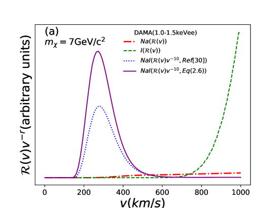
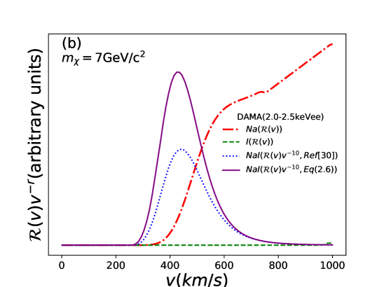
Figure 1: DAMA ADM response functions $\mathcal{R}$ as defined in Eq (3.8) for $m_{\chi}=7~{}{\rm GeV}/c^{2}$ in two energy bins: (a) $1~{}{\rm keVee}<E^{\prime}<1.5~{}{\rm keVee}$, and (b) $2~{}{\rm keVee}<E^{\prime}<2.5~{}{\rm keVee}$. In each plot the dot–dashed lines (red) and the dashed lines (green) represent the sodium and the iodine contribution, respectively. The solid purple line shows the function $v^{-10}\mathcal{R}$ for NaI used in the regularization procedure of Eq. (3.16), when the magnetic contribution to the WIMP–sodium cross section is calculated using Eq. (2.6). The dotted line (blue) shows the same quantity but computed using the shell–model calculations of the nuclear structure functions in [32], Eq. (2.9).

3.1 Maxwellian velocity distribution

In this Section we assume that the WIMP velocity distribution in the Galactic rest frame is a standard isotropic Maxwellian at rest, truncated at the escape velocity $v_{\rm esc}$,

$$f_{\rm gal}(u)=\frac{1}{\pi^{3/2}v_{0}^{3}N_{\rm esc}}\,e^{-u^{2}/v_{0}^{2}}\,\Theta(v_{\rm esc}-u).$$ (3.11)

Here $u$ is the WIMP speed in the Galactic rest frame, $\Theta$ is the Heaviside step function, and

$$N_{\rm esc}=\mbox{erf}(z)-2\,z\,e^{-z^{2}}/\pi^{1/2}$$ (3.12)

with $z=v_{\rm esc}/v_{0}$. The WIMP speed distribution in the laboratory frame can be obtained with a change of reference frame. It depends on the speed of the Earth with respect to the Galactic rest frame, which neglecting the ellipticity of the Earth orbit, is given by

$$v_{E}(t) =\big{[}v_{\odot}^{2}+v_{\oplus}^{2}+2\,v_{\odot}\,v_{\oplus}\,\cos\gamma\,\cos[\omega(t-t_{0})]\big{]}^{1/2}.$$ (3.13)

In this formula, $v_{\odot}$ is the speed of the Sun in the Galactic rest frame, $v_{\oplus}$ is the speed of the Earth relative to the Sun, and $\gamma$ is the ecliptic latitude of the Sun’s motion in the Galaxy. We take $\cos\gamma\simeq 0.49$, $v_{\oplus}=2\pi(1~{}{\rm AU})/(1~{}{\rm year})\simeq 29~{}{\rm km/s}$, $v_{\odot}=v_{0}+12~{}{\rm km/s}$, $v_{0}=220~{}{\rm km/s}$ [34], and $v_{esc}=550~{}{\rm km/s}$ [35].

The velocity integral $\eta(v_{\rm min},t)$ for the truncated Maxwellian distribution can finally be computed from the expression of the speed distribution. We have obtained its modulated and unmodulated parts by expanding $\eta(v_{\rm min},t)$ to first order in $v_{\oplus}/v_{\odot}$.

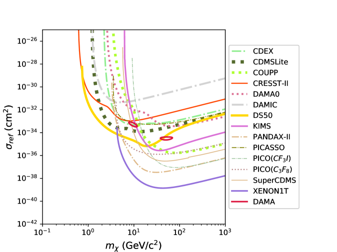
Figure 2: Anapole Dark Matter $5\sigma$ DAMA modulation regions in the $m_{\chi}$–$\sigma_{\rm ref}$ plane (inside the two closed solid red lines) when the WIMP velocity distribution is taken as a standard Maxwellian, and 90% C.L. upper bounds on $\sigma_{\rm ref}$ from other DM direct searches (other lines).

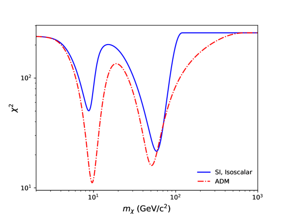
Figure 3: Minimum of $\chi^{2}(m_{\chi},\sigma_{\rm ref})$ in Eq. (3.14) at fixed $m_{\chi}$ for anapole dark matter (red dot–dashed line) and a spin-independent isoscalar interaction (blue solid line).

The expected modulation amplitude $S_{{\rm m},k}$ in the $k$-th DAMA bin depends on the WIMP mass $m_{\chi}$ and on the reference cross section $\sigma_{\rm ref}$ (actually, on the product $\sigma_{\rm ref}\rho_{\chi}$; we use a reference value $\rho_{\chi}=0.3~{}{\rm GeV}/c^{2}/{\rm cm}^{3}$). To check how well ADM with a Maxwellian distribution fits the DAMA/LIBRA–phase2 data $S^{\rm exp}_{{\rm m},k}\pm\sigma_{k}$ in [11], we perform a $\chi^{2}$ analysis constructing the quantity

$$\chi^{2}(m_{\chi},\sigma_{\rm ref})=\sum_{k=1}^{15}\frac{\left[S_{{\rm m},k}(m_{\chi},\sigma_{\rm ref})-S^{\rm exp}_{{\rm m},k}\right]^{2}}{\sigma_{k}^{2}}.$$ (3.14)

We consider 14 energy bins of width 0.5 keVee from 1 keVee to 8 keVee, and one wider high–energy control bin extending from 8 keVee to 16 keVee.

The global minimum of $\chi^{2}(m_{\chi},\sigma_{\rm ref})$ for ADM occurs at $m_{\chi}=9.6~{}{\rm GeV}/c^{2}$, $\sigma_{\rm ref}=5.5\times 10^{-34}~{}{\rm cm}^{2}$, and its value is $\chi^{2}_{min}=11.1$ ($\text{$p$-value}=0.602$ with $15-2$ degrees of freedom, which is an indication of a good fit).

The $5\sigma$ DAMA modulation regions are plotted in Fig. 2 as the two regions inside the contour $\chi^{2}(m_{\chi},\sigma_{\rm ref})=\chi^{2}_{min}+5^{2}$ in the $m_{\chi}$–$\sigma_{\rm ref}$ plane. The region at lower masses (around $m_{\chi}\approx 10~{}{\rm GeV}/c^{2}$ and $\sigma_{\rm ref}\approx 10^{-33}~{}{\rm cm}^{2}$) contains the global minimum of the $\chi^{2}$. The region at higher masses (around $m_{\chi}\approx 50~{}{\rm GeV}/c^{2}$ and $\sigma_{\rm ref}\approx 3\times 10^{-35}~{}{\rm cm}^{2}$) contains a secondary local minimum. The other lines in Fig. 2 are the 90% upper bounds from other existing DM direct–detection experiments (the region above each line is excluded). As expected, and in agreement with [6], a DAMA explanation in terms of ADM is excluded by the null results of other experiments, for a Maxwellian WIMP velocity distribution.

In the rest of this section we compare the ADM $\chi^{2}$ to the $\chi^{2}$ of the often-quoted isoscalar spin-independent case, and we comment on the relative importance of scattering off sodium vs iodine.

In Fig. 3, the minimum of $\chi^{2}(m_{\chi},\sigma_{\rm ref})$ in Eq. (3.14) at fixed $m_{\chi}$ is plotted as a dot–dashed line (red) as a function of $m_{\chi}$ (this is the $\chi^{2}$ obtained by profiling out $\sigma_{\rm ref}$). The global minimum around $m_{\chi}\approx 10~{}{\rm GeV}/c^{2}$ and the secondary minimum around $m_{\chi}\approx 50~{}{\rm GeV}/c^{2}$ are clearly visible. Fig. 3 also shows (solid blue line) the minimum of the $\chi^{2}$ at fixed $m_{\chi}$ for an isoscalar spin-independent (SI) cross section, which scales with the square of the nuclear mass number. Also in this case two local minima are present. However now the absolute minimum is the one with the largest mass [12], while the low–mass local minimum at $m_{\chi}$=8.8 GeV/c² has a $\chi^{2}$ significantly larger ($\chi^{2}_{min}=50.3$) than in the ADM case.

The different behavior of the $\chi^{2}$ in the ADM and SI cases can be understood from the different hierarchy of the WIMP–iodine and WIMP–sodium cross sections in the two cases. In fact, differently from the situation with DAMA–phase1, in the two additional low–energy bins from 1 keVee to 2 keVee of DAMA–phase2 the modulation effect receives a contribution from WIMP scattering off iodine targets also at low WIMP masses (below $10~{}{\rm GeV}/c^{2}$). This can be seen in Fig. 1(a) for $m_{\chi}$=7 GeV/c², where for 1 keVee$<E^{\prime}<$1.5 keVee the contribution to $\mathcal{R}$ from WIMP–iodine scattering is different from zero when $v_{\rm min}\mathrel{\mathop{\kern 0.0pt\hbox to0.0pt{\raise 0.86108pt\hbox{$>$}\hss}}\lower 3.87495pt\hbox{\kern-1.90002pt$\sim$}}$ 700 km/s, a range below the escape velocity in the lab frame (for our standard choice of the astrophysical parameters summarized after Eq. (3.13)). On the other hand, as shown in Fig. 1(b), for the same WIMP mass and for $2~{}{\rm keVee}<E^{\prime}<2.5~{}{\rm keVee}$ (i.e., in the lowest energy bin of DAMA–phase1) WIMP–iodine scattering does not contribute to the expected signal until the WIMP speed is well above the escape velocity. For SI interactions, due to the large hierarchy between the WIMP–iodine and WIMP–sodium cross sections, the additional contribution from WIMP–iodine scattering is known to lead to a steep rise of the expected modulation amplitudes for $E^{\prime}<2~{}{\rm keVee}$. This rise is incompatible with the DAMA–phase2 measurements, worsening considerably the goodness–of–fit in going from DAMA–phase1 to DAMA–phase2 [12, 13]. On the other hand, in the case of ADM, for low WIMP masses the cross section in Eq. (2.3) takes its dominant contribution from the magnetic component in sodium. This can be seen by examining the NaI response functions $\mathcal{R}$ in Fig. 1. The response functions $\mathcal{R}$ (appropriately multiplied by the factor $v^{-10}$, see next Section) are the solid purple line when $F^{2}_{\rm m,Na}(q^{2})$ is evaluated using Eq.(2.6), and the dotted line (blue) when $F^{2}_{\rm m,Na}(q^{2})$ is evaluated using the nuclear structure functions of Ref. [32]. As pointed out in Section 2, the form factors in [32] largely underestimate the measured sodium magnetic moment, so that in such case the WIMP–sodium cross section is only due to the electric part. Thus, in Fig. 1, the difference between the two evaluations of $\mathcal{R}$ (solid purple line vs dotted blue line) is due to the magnetic component in sodium. This implies that for ADM, when the magnetic contribution of Na is included, it is the dominant one. In particular, near the absolute minimum of the $\chi^{2}$, the enhancement of the sodium contribution due to the magnetic component of the cross section reduces the hierarchy between the ADM WIMP–iodine and WIMP–sodium cross sections compared to the SI case. It is this that produces a fit of better quality. The ADM $\chi^{2}$ in Fig. 3 also shows a milder rise at large $m_{\chi}$ compared to the SI interaction. This is a general property of models for which the cross section depends explicitly on the WIMP incoming velocity. This kind of models provides a better fit to the DAMA modulation data at large values of $m_{\chi}$ than models with a velocity–independent cross–section, due to the different phase of the modulation amplitudes [13].

3.2 Halo–independent analysis

In the halo–independent method of Refs. [33, 6], measured rates $R^{i}_{[E^{\prime}_{1},E^{\prime}_{2}]}$ (with $i=0,1$) are mapped into suitable averages of the two halo functions $\tilde{\eta}^{i}$. Ref. [33] defines averages $\overline{\tilde{\eta}^{i}}_{[v_{{\rm min},1},v_{{\rm min},2}]}$ ($i=0,1$) using $\mathcal{R}(v_{\rm min})$ in Eq. (3.8) as a weight function,

$$\overline{\tilde{\eta}^{i}}_{[v_{{\rm min},1},v_{{\rm min},2}]}=\frac{\int_{0}^{\infty}\text{d}v_{\rm min}\,\tilde{\eta}^{i}(v_{\rm min})\,\mathcal{R}_{[E^{\prime}_{1},E^{\prime}_{2}]}(v_{\rm min})}{\int_{0}^{\infty}\text{d}v_{\rm min}\,\mathcal{R}_{[E^{\prime}_{1},E^{\prime}_{2}]}(v_{\rm min})}.$$ (3.15)

The velocity intervals $[v_{{\rm min},1},v_{{\rm min},2}]$ are defined as those velocity intervals where the weight function $\mathcal{R}_{[E^{\prime}_{1},E^{\prime}_{2}]}(v_{\rm min})$ is sizeably different from zero.

In the case of ADM, the integral in the denominator of Eq. (3.15) diverges because the differential cross section in Eq. (2.3) depends on a power of $v$ larger than $-2$. Ref. [6] found a solution to this complication by using the weight functions $v_{\rm min}^{-r}\mathcal{R}(v_{\rm min})$ in place of $\mathcal{R}(v_{\rm min})$, where $r$ is a suitable integer. Regularized averages of $\tilde{\eta}^{i}$ ($i=0,1$) are defined as

$$v_{\rm min}^{-r}\langle v_{\rm min}^{r}\tilde{\eta}^{i}\rangle_{[v_{{\rm min},1},v_{{\rm min},2}]}=\frac{\int_{0}^{\infty}\text{d}v_{\rm min}\,v_{\rm min}^{r}\,\tilde{\eta}^{i}(v_{\rm min})\,w^{(r)}_{[E^{\prime}_{1},E^{\prime}_{2}]}(v_{\rm min})}{v_{\rm min}^{r}\int_{0}^{\infty}\text{d}v_{\rm min}\,w^{(r)}_{[E^{\prime}_{1},E^{\prime}_{2}]}(v_{\rm min})},$$ (3.16)

where

$$w^{(r)}_{[E^{\prime}_{1},E^{\prime}_{2}]}(v_{\rm min})=v_{\rm min}^{-r}\,\mathcal{R}_{[E^{\prime}_{1},E^{\prime}_{2}]}(v_{\rm min}).$$ (3.17)

The velocity intervals $[v_{{\rm min},1},v_{{\rm min},2}]$ are defined as those velocity intervals where the weight function $w^{(r)}_{[E^{\prime}_{1},E^{\prime}_{2}]}(v_{\rm min})$ is sizeably different from zero.

Estimates of the regularized averages $v_{\rm min}^{-r}\langle v_{\rm min}^{r}\tilde{\eta}^{i}\rangle_{[v_{{\rm min},1},v_{{\rm min},2}]}$ from measurements $R^{i}_{[E^{\prime}_{1},E^{\prime}_{2}]}$ are obtained by noticing that the numerator in Eq. (3.16) is equal to the numerator in Eq. (3.15) and is equal to $R^{i}_{[E^{\prime}_{1},E^{\prime}_{2}]}$ by Eqs. (3.6) and (3.10),

$$v_{\rm min}^{-r}\langle v_{\rm min}^{r}\tilde{\eta}^{i}\rangle_{[v_{{\rm min},1},v_{{\rm min},2}]}=\frac{R^{i}_{[E^{\prime}_{1},E^{\prime}_{2}]}}{v_{\rm min}^{r}\int_{0}^{\infty}\text{d}v_{\rm min}\,v_{\rm min}^{-r}\,\mathcal{R}_{[E^{\prime}_{1},E^{\prime}_{2}]}(v_{\rm min})}.$$ (3.18)

For the DAMA modulation, estimates of $\tilde{\eta}^{1}$ as the regularized average $v_{\rm min}^{-r}\langle v_{\rm min}^{r}\tilde{\eta}^{1}\rangle_{[v_{{\rm min},1},v_{{\rm min},2}]}$ with $r=10$ are shown as crosses in Figs. 4, 5 and 6, where $m_{\chi}=5$, 7 and $10~{}{\rm GeV}/c^{2}$, respectively. In these figures we show the DAMA modulation amplitude in the first 6 energy bins of [11] from 1 keVee to 6 keVee, where the modulation signal is concentrated. To determine the $v_{\rm min}$ interval corresponding to each detected energy interval $[E^{\prime}_{1},E^{\prime}_{2}]$ in DAMA we choose to use $68\%$ central quantile intervals of the modified response function $w^{(r)}_{[E^{\prime}_{1},E^{\prime}_{2}]}(v_{\rm min})$, i.e,, we determine ${v_{\rm min}}_{,1}$ and ${v_{\rm min}}_{,2}$ such that the areas under the function $v_{\rm min}^{-r}\mathcal{R}_{[E^{\prime}_{1},E^{\prime}_{2}]}(v_{\rm min})$ to the left of ${v_{\rm min}}_{,1}$ and to the right of ${v_{\rm min}}_{,2}$ are each separately $16\%$ of the total area under the function. This gives the horizontal width of the crosses corresponding to the rate measurements in Figs. 4, 5 and 6. On the other hand, the horizontal placement of the vertical bar in the crosses corresponds to the average of $v_{\rm min}$ using weights $w^{(r)}_{[E^{\prime}_{1},E^{\prime}_{2}]}(v_{\rm min})$, i.e., $v_{\rm min}(\text{vertical bar})=\big{[}\int_{0}^{\infty}\text{d}v_{\rm min}\,v_{\rm min}^{1-r}\mathcal{R}_{[E^{\prime}_{1},E^{\prime}_{2}]}(v_{\rm min})\big{]}/\big{[}\int_{0}^{\infty}\text{d}v_{\rm min}\,v_{\rm min}^{-r}\mathcal{R}_{[E^{\prime}_{1},E^{\prime}_{2}]}(v_{\rm min})\big{]}$. The extension of the vertical bar shows the $1\sigma$ interval around the central value of the measured rate.

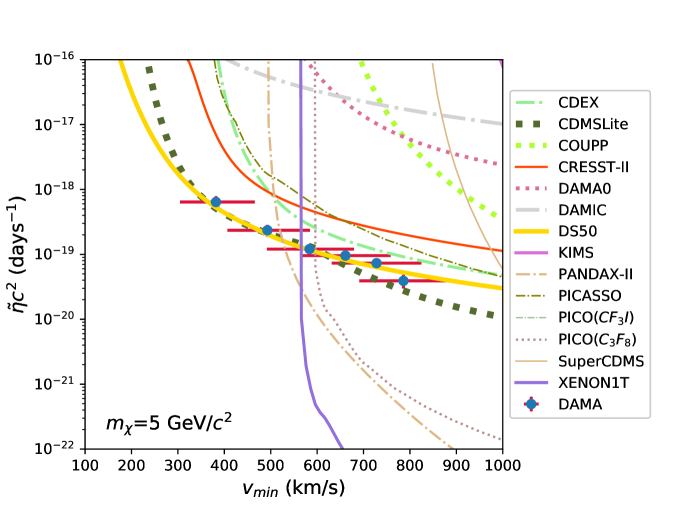
Figure 4: Measurements of $v_{\rm min}^{-10}\langle v_{\rm min}^{10}\tilde{\eta}^{1}(v_{\rm min})\rangle$ (DAMA) and upper bounds on $\tilde{\eta}^{0}$ (other experiments) for anapole dark matter with $m_{\chi}=5~{}{\rm GeV}/c^{2}$.

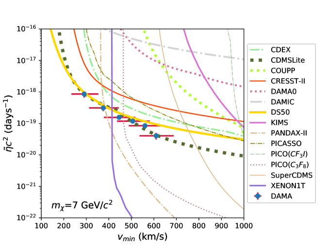
Figure 5: Same as Fig.4 but for $m_{\chi}=7~{}{\rm GeV}/c^{2}$.

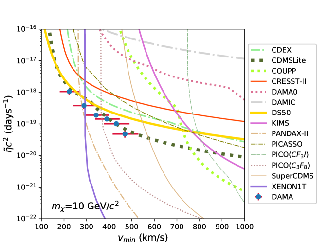
Figure 6: Same as Fig.4 but for $m_{\chi}=10~{}{\rm GeV}/c^{2}$.

.

To compute upper bounds on $\tilde{\eta}^{\,0}$ from upper limits $R_{[E^{\prime}_{1},E^{\prime}_{2}]}^{\rm lim}$ on the unmodulated rates, we follow the conservative procedure in Ref. [36]. Since $\tilde{\eta}^{\,0}(v_{\rm min})$ is by definition a non-decreasing function, the lowest possible $\tilde{\eta}^{0}(v_{\rm min})$ function passing through a point $(v_{0},\tilde{\eta}^{\,0})$ in $v_{\rm min}$ space is the downward step function $\tilde{\eta}^{0}\,\theta(v_{0}-v_{\rm min})$. The maximum value of $\tilde{\eta}^{0}$ allowed by a null experiment at a certain confidence level, denoted by $\tilde{\eta}^{\rm lim}(v_{0})$, is then determined by the experimental limit on the rate $R_{[E^{\prime}_{1},E^{\prime}_{2}]}^{\rm lim}$ as

$$\tilde{\eta}^{\rm lim}(v_{0})=\frac{R^{\rm lim}_{[E^{\prime}_{1},E^{\prime}_{2}]}}{\int_{0}^{v_{0}}\text{d}v_{\rm min}\,\mathcal{R}_{[E^{\prime}_{1},E^{\prime}_{2}]}(v_{\rm min})}\ .$$ (3.19)

These upper limits are shown as continuous lines in Figs. 4, 5 and 6 for the experiments listed there and in Appendix A.

We see that the DAMA points lie either in the excluded region or just at its boundary (determined by the constraints from DS50, CDMSLite, PANDAX–II and XENON1T). The best we could find in terms of compatibility between DAMA and the other experiments are the two lowest energy DAMA bins barely outside the excluded region at $m_{\chi}\approx 7$–$8~{}{\rm GeV}/c^{2}$. In particular, it appears impossible to explain all modulated bins in DAMA with anapole dark matter and at the same time account for the other null direct DM search results, even in the context of a halo-independent analysis. This is in sharp contrast to the situation four years ago when anapole dark matter was still viable when analyzed in a halo–independent way [6].

To be pedantic, one could object that we are actually comparing two quantities defined differently for the modulated and unmodulated parts of the DM signal, namely Eq. (3.18) and Eq. (3.19). For the two lowest DAMA energy bins that lie near the boundary of the excluded region in Figs. 4–6 (near the CDMSlite, DS50, and PANDAX-II upper limits), one may want to consider more sophisticated analysis methods in which such objection is avoided (e.g., the method of Ref. [37]). On the other hand, the DAMA bins above 2 keVee are excluded by XENON1T, PANDAX-II, and PICO(C₃F₈) by several orders of magnitude, and a more sophisticated analysis is not warranted.

4 Conclusions

We have re–examined the case of anapole dark matter as an explanation for the DAMA annual modulation in light of the DAMA/LIBRA–phase2 results and improved upper limits from other DM searches.

For a Maxwellian WIMP velocity distribution, anapole dark matter is unable to provide an explanation of the DAMA modulation compatible with the other direct DM search results. Nevertheless, anapole dark matter provides a better fit to the DAMA–phase2 modulation data than a a standard isoscalar spin–independent interaction. This is due to the contribution from the magnetic moment of sodium, which reduces the hierarchy between the ADM WIMP–iodine and WIMP–sodium cross sections compared to the SI case.

A halo-independent analysis shows that explaining the DAMA modulation above 2 keVee in terms of anapole dark matter is basically impossible in the face of the null results of XENON1T, PANDAX-II, and PICO(C₃F₈). On the other hand, the DAMA/LIBRA–phase2 modulation measurements below 2 keVee lie near the border of the excluded region.

We conclude that in light of current measurements, anapole dark matter does not seem to be a viable explanation for the totality of the DAMA modulation, not even in a halo–independent analysis, although the DAMA/LIBRA–phase2 modulation measurements below 2 keVee are marginally allowed.

Appendix A Experiments

In our analysis we have included an extensive list of updated constraints from existing DM direct-search experiments: CDEX [14], CDMSlite [15], COUPP [16], CRESST-II [17, 18], DAMIC [19], DAMA (modulation data [38, 3, 4, 11] and average count rate [39], indicated as DAMA0 in the plots), DarkSide–50 [20] (indicated as DS50 in the plots), KIMS [21], PANDAX-II [22], PICASSO [23], PICO-60 (using a CF₃I target [24] and a C₃F₈ target [25]), SuperCDMS [26] and XENON1T [27]. With the exception of the latest result from XENON1T [28], the details of the treatment of the other constraints are provided in the Appendix of  [40]. For XENON1T (2018 analysis), we have assumed 7 WIMP candidate events in the range of 3PE $\leq S_{1}\leq$ 70PE, as shown in Fig. 3 of Ref. [28] for the primary scintillation signal S1 (directly in Photo Electrons, PE), with an exposure of 278.8 days and a fiducial volume of 1.3 ton of xenon. We have used the efficiency taken from Fig. 1 of [28] and employed a light collection efficiency $g_{1}$=0.055; for the light yield $L_{y}$ we have extracted the best estimation curve for photon yields $\langle n_{ph}\rangle/E$ from Fig. 7 in [41] with an electric field of $90~{}{\rm V/cm}$.

References

- [1] Planck Collaboration, P. A. R. Ade et al., Planck 2013 results. XVI. Cosmological parameters, Astron. Astrophys. 571 (2014) A16, [arXiv:1303.5076].
- [2] A. K. Drukier, K. Freese, and D. N. Spergel, Detecting Cold Dark Matter Candidates, Phys. Rev. D33 (1986) 3495–3508.
- [3] DAMA Collaboration, R. Bernabei et al., First results from DAMA/LIBRA and the combined results with DAMA/NaI, Eur. Phys. J. C56 (2008) 333–355, [arXiv:0804.2741].
- [4] DAMA, LIBRA Collaboration, R. Bernabei et al., New results from DAMA/LIBRA, Eur. Phys. J. C67 (2010) 39–49, [arXiv:1002.1028].
- [5] R. Bernabei et al., Final model independent result of DAMA/LIBRA-phase1, Eur. Phys. J. C73 (2013) 2648, [arXiv:1308.5109].
- [6] E. Del Nobile, G. B. Gelmini, P. Gondolo, and J.-H. Huh, Direct detection of Light Anapole and Magnetic Dipole DM, JCAP 1406 (2014) 002, [arXiv:1401.4508].
- [7] C. M. Ho and R. J. Scherrer, Anapole Dark Matter, Phys. Lett. B722 (2013) 341–346, [arXiv:1211.0503].
- [8] A. L. Fitzpatrick and K. M. Zurek, Dark Moments and the DAMA-CoGeNT Puzzle, Phys. Rev. D82 (2010) 075004, [arXiv:1007.5325].
- [9] M. T. Frandsen, F. Kahlhoefer, C. McCabe, S. Sarkar, and K. Schmidt-Hoberg, The unbearable lightness of being: CDMS versus XENON, JCAP 1307 (2013) 023, [arXiv:1304.6066].
- [10] M. I. Gresham and K. M. Zurek, Light Dark Matter Anomalies After LUX, Phys. Rev. D89 (2014), no. 1 016017, [arXiv:1311.2082].
- [11] R. Bernabei et al., First model independent results from DAMA/LIBRA-phase2, arXiv:1805.10486.
- [12] S. Baum, K. Freese, and C. Kelso, Dark Matter implications of DAMA/LIBRA-phase2 results, arXiv:1804.01231.
- [13] S. Kang, S. Scopel, G. Tomar, and J.-H. Yoon, DAMA/LIBRA-phase2 in WIMP effective models, JCAP 1807 (2018), no. 07 016, [arXiv:1804.07528].
- [14] CDEX Collaboration, L. T. Yang et al., Limits on light WIMPs with a 1 kg-scale germanium detector at 160 eVee physics threshold at the China Jinping Underground Laboratory, Chin. Phys. C42 (2018), no. 2 023002, [arXiv:1710.06650].
- [15] SuperCDMS Collaboration, R. Agnese et al., Low-mass dark matter search with CDMSlite, Phys. Rev. D97 (2018), no. 2 022002, [arXiv:1707.01632].
- [16] COUPP Collaboration, E. Behnke et al., First Dark Matter Search Results from a 4-kg CF3I Bubble Chamber Operated in a Deep Underground Site, Phys. Rev. D86 (2012), no. 5 052001, [arXiv:1204.3094]. [Erratum: Phys. Rev.D90,no.7,079902(2014)].
- [17] CRESST Collaboration, G. Angloher et al., Results on light dark matter particles with a low-threshold CRESST-II detector, Eur. Phys. J. C76 (2016), no. 1 25, [arXiv:1509.01515].
- [18] CRESST Collaboration, G. Angloher et al., Description of CRESST-II data, arXiv:1701.08157.
- [19] DAMIC Collaboration, A. Aguilar-Arevalo et al., Search for low-mass WIMPs in a 0.6 kg day exposure of the DAMIC experiment at SNOLAB, Phys. Rev. D94 (2016), no. 8 082006, [arXiv:1607.07410].
- [20] DarkSide Collaboration, P. Agnes et al., Low-mass Dark Matter Search with the DarkSide-50 Experiment, arXiv:1802.06994.
- [21] H. S. Lee et al., Search for Low-Mass Dark Matter with CsI(Tl) Crystal Detectors, Phys. Rev. D90 (2014), no. 5 052006, [arXiv:1404.3443].
- [22] PandaX-II Collaboration, X. Cui et al., Dark Matter Results From 54-Ton-Day Exposure of PandaX-II Experiment, Phys. Rev. Lett. 119 (2017), no. 18 181302, [arXiv:1708.06917].
- [23] E. Behnke et al., Final Results of the PICASSO Dark Matter Search Experiment, Astropart. Phys. 90 (2017) 85–92, [arXiv:1611.01499].
- [24] PICO Collaboration, C. Amole et al., Dark Matter Search Results from the PICO-60 CF3I Bubble Chamber, Submitted to: Phys. Rev. D (2015) [arXiv:1510.07754].
- [25] PICO Collaboration, C. Amole et al., Dark Matter Search Results from the PICO-60 C3F8 Bubble Chamber, Phys. Rev. Lett. 118 (2017), no. 25 251301, [arXiv:1702.07666].
- [26] SuperCDMS Collaboration, R. Agnese et al., Results from the Super Cryogenic Dark Matter Search Experiment at Soudan, Phys. Rev. Lett. 120 (2018), no. 6 061802, [arXiv:1708.08869].
- [27] XENON Collaboration, E. Aprile et al., First Dark Matter Search Results from the XENON1T Experiment, Phys. Rev. Lett. 119 (2017), no. 18 181301, [arXiv:1705.06655].
- [28] XENON Collaboration, E. Aprile et al., Dark Matter Search Results from a One TonneYear Exposure of XENON1T, arXiv:1805.12562.
- [29] R. H. Helm, Inelastic and Elastic Scattering of 187-Mev Electrons from Selected Even-Even Nuclei, Phys. Rev. 104 (1956) 1466–1475.
- [30] T. W. Donnelly and I. Sick, ELASTIC MAGNETIC ELECTRON SCATTERING FROM NUCLEI, Rev. Mod. Phys. 56 (1984) 461–566.
- [31] A. L. Fitzpatrick, W. Haxton, E. Katz, N. Lubbers, and Y. Xu, The Effective Field Theory of Dark Matter Direct Detection, JCAP 1302 (2013) 004, [arXiv:1203.3542].
- [32] N. Anand, A. L. Fitzpatrick, and W. C. Haxton, Weakly interacting massive particle-nucleus elastic scattering response, Phys. Rev. C89 (2014), no. 6 065501, [arXiv:1308.6288].
- [33] E. Del Nobile, G. Gelmini, P. Gondolo, and J.-H. Huh, Generalized Halo Independent Comparison of Direct Dark Matter Detection Data, JCAP 1310 (2013) 048, [arXiv:1306.5273].
- [34] S. E. Koposov, H.-W. Rix, and D. W. Hogg, Constraining the Milky Way potential with a 6-D phase-space map of the GD-1 stellar stream, Astrophys. J. 712 (2010) 260–273, [arXiv:0907.1085].
- [35] T. Piffl et al., The RAVE survey: the Galactic escape speed and the mass of the Milky Way, Astron. Astrophys. 562 (2014) A91, [arXiv:1309.4293].
- [36] P. J. Fox, J. Liu, and N. Weiner, Integrating Out Astrophysical Uncertainties, Phys. Rev. D83 (2011) 103514, [arXiv:1011.1915].
- [37] P. Gondolo and S. Scopel, Halo-independent determination of the unmodulated WIMP signal in DAMA: the isotropic case, JCAP 1709 (2017), no. 09 032, [arXiv:1703.08942].
- [38] R. Bernabei et al., Searching for WIMPs by the annual modulation signature, Phys. Lett. B424 (1998) 195–201.
- [39] DAMA Collaboration, R. Bernabei et al., The DAMA/LIBRA apparatus, Nucl. Instrum. Meth. A592 (2008) 297–315, [arXiv:0804.2738].
- [40] S. Kang, S. Scopel, G. Tomar, and J.-H. Yoon, Present and projected sensitivities of Dark Matter direct detection experiments to effective WIMP-nucleus couplings, arXiv:1805.06113.
- [41] XENON Collaboration, E. Aprile et al., Signal Yields of keV Electronic Recoils and Their Discrimination from Nuclear Recoils in Liquid Xenon, Phys. Rev. D97 (2018), no. 9 092007, [arXiv:1709.10149].