Robot Safe Interaction System
for Intelligent Industrial Co-Robots

Abstract

Human-robot interactions have been recognized to be a key element of future industrial collaborative robots (co-robots). Unlike traditional robots that work in structured and deterministic environments, co-robots need to operate in highly unstructured and stochastic environments. To ensure that co-robots operate efficiently and safely in dynamic uncertain environments, this paper introduces the robot safe interaction system. In order to address the uncertainties during human-robot interactions, a unique parallel planning and control architecture is proposed, which has a long term global planner to ensure efficiency of robot behavior, and a short term local planner to ensure real time safety under uncertainties. In order for the robot to respond immediately to environmental changes, fast algorithms are used for real-time computation, i.e., the convex feasible set algorithm for the long term optimization, and the safe set algorithm for the short term optimization. Several test platforms are introduced for safe evaluation of the developed system in the early phase of deployment. The effectiveness and the efficiency of the proposed method have been verified in experiment with an industrial robot manipulator.

I Introduction

Human-robot interactions (HRI) have been recognized to be a key element of future robots in many application domains, which entail huge social and economical impacts [6, 4]. Future robots are envisioned to function as human’s counterparts, which are independent entities that make decisions for themselves; intelligent actuators that interact with the physical world; and involved observers that have rich senses and critical judgements. Most importantly, they are entitled social attributions to build relationships with humans [9]. We call these robots co-robots. In particular, this paper focuses on industrial co-robots.

In modern factories, human workers and robots are two major workforces. For safety concerns, the two are normally separated with robots confined in metal cages, which limits the productivity as well as the flexibility of production lines. In recent years, attention has been directed to remove the cages so that human workers and robots may collaborate to create a human-robot co-existing factory [5]. Manufacturers are interested in combining human’s flexibility and robot’s productivity in flexible production lines [15]. The potential benefits of industrial co-robots are huge and extensive. They may be placed in human-robot teams in flexible production lines [16] as shown in Fig. 1, where robot arms and human workers cooperate in handling workpieces, and automated guided vehicles (AGV) co-inhabit with human workers to facilitate factory logistics [32]. Automotive manufacturers Volkswagen and BMW [1] have taken the lead to introduce human-robot cooperation in final assembly lines in 2013.

In the factories of the future, more and more human-robot interactions are anticipated to take place. Unlike traditional robots that work in structured and deterministic environments, co-robots need to operate in highly unstructured and stochastic environments. The fundamental problem is how to ensure that co-robots operate efficiently and safely in dynamic uncertain environments.

New ISO standards has been developed concerning these new applications [13]. Several safe cooperative robots or co-robots have been released [2], such as Green Robot from FANUC (Japan), UR5 from Universal Robots (Denmark), Baxter from Rethink Robotics (US), NextAge from Kawada (Japan), and WorkerBot from Pi4_Robotics GmbH (Germany). However, many of these products focus on intrinsic safety, i.e. safety in mechanical design [14], actuation [34] and low level motion control [29]. Safety during interactions with humans, which are key to intelligence (including perception, cognition and high level motion planning and control), still needs to be explored.

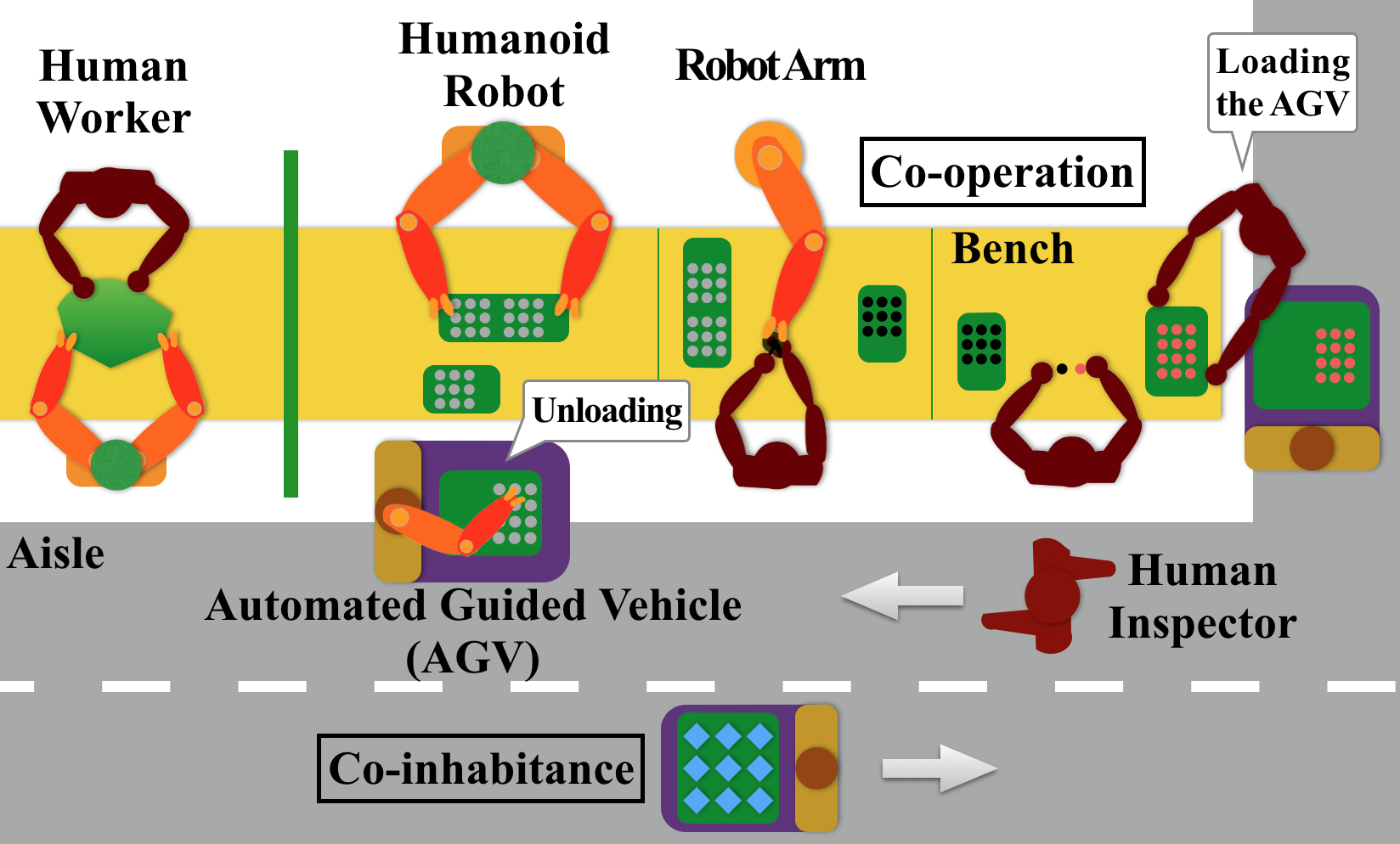
Figure 1: Human-robot interactions in future production lines.

Technically, it is challenging to design the behavior of industrial co-robots. In order to make the industrial co-robots human-friendly, they should be equipped with the abilities [12] to: collect environmental data and interpret such data, adapt to different tasks and different environments, and tailor itself to the human workers’ needs. The challenges are (i) coping with complex and time-varying human motion, and (ii) assurance of real time safety without sacrificing efficiency.

This paper introduces the robot safe interaction system (RSIS), which establishes a methodology to design the robot behavior to safely and efficiently interact with humans. In order to address the uncertainties during human-robot interactions, a unique parallel planning and control architecture is introduced, which has a long term global planner to ensure efficiency of robot behavior, and a short term local planner to ensure real time safety under uncertainties. The parallel planner integrates fast algorithms for real-time motion planning, e.g. the convex feasible set algorithm (CFS) [21] for the long term planning, and the safe set algorithm (SSA) [23] for the short term planning.

An early version of the work has been discussed in [26], where the long-term planner does not consider moving obstacles (humans) in the environment. The interaction with humans is solely considered in the short-term planner. This method has low computation complexity, as the long term planning problem becomes time-invariant and can be solved offline. However, the robot may be trapped into local optima due to lack of global perspective in the long term. Nonetheless, with the introduction of CFS, long term planning can be handled efficiently in real time. Hence this paper considers interactions with humans in both planners.

This paper contributes in the following four aspects. First, it proposes an integrated framework to design robot behaviors, which includes a macroscopic multi-agent model and a microscopic behavior model. Second, it introduces a unique parallel planning architecture that integrates previously developed algorithms to handle both safety and efficiency under system uncertainty and computation limits. Third, two kinds of evaluation platforms for human-robot interactions are introduced to protect human subjects in the early phase of development. Last, the proposed RSIS has been integrated and tested on robot hardware, which validates its effectiveness. It is worth noting that safety is only guaranteed under certain assumptions of human behaviors. For a robot arm with fixed base, there is always a way to collide with it, especially intentionally. For industrial practice, RSIS should be placed on top of other intrinsic safety mechanisms mentioned earlier to ensure safety even when collision happens. Moreover, dual channel implementation of RSIS may be considered to ensure reliability.

The remainder of the paper is organized as follows. Section II formulates the problem. Section III proposes RSIS. Section IV discusses SSA for short term planning, while Section V discusses CFS for long term planning. Section VI introduces the evaluation platforms. Experiment results with those platforms are shown in Section VII. Section VIII points out future directions. Section IX concludes the paper.

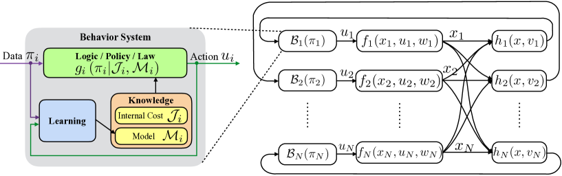
Figure 2: The block diagram of the decomposable multi-agent system.

II Problem Formulation

Behavior is the way in which one acts or conducts oneself, especially toward others. This section introduces a multi-agent framework to model human-robot interactions. Behavior models are encoded in the multi-agent model. This paper studies the methodology of behavior design, i.e., how to realize the design goal (to ensure that co-robots operate efficiently and safely in dynamic uncertain environments) within the design scope (the inputs and outputs of the robotic system).

II-A Macroscopic Multi-Agent Model

An agent is an entity that perceives and acts, whose behavior is determined by a behavior system. Human-robot interactions can be modeled in a multi-agent framework [23] where robots and humans are all regarded as agents. If a group of robots are coordinated by one central decision maker, they are regarded as one agent.

Suppose there are $N$ agents in the environment and are indexed from $1$ to $N$. Denote agent $i$’s state as $x_{i}$, its control input as $u_{i}$, its data set as $\pi_{i}$ for $i=1,...,N$. The physical interpretations of the state, input and data set for different plants in different scenarios vary. For robot arm, the state can be joint position and joint velocity, and the input can be joint torque. For automated guided vehicle, the state can be vehicle position and heading, and the input can be throttle and pedal angle. When communication is considered, the state may also include the transmitted information and the input can be the action to send information. Let $x_{e}$ be the state of the environment. Denote the system state as $x=[x_{1};\ldots;x_{N};x_{e}]\in X$ where $X$ is the state space of the system.

Every agent $i$ has its dynamics,

$$\dot{x}_{i}=f_{i}(x_{i},u_{i},w_{i}),$$ (1)

where $w_{i}$ is a noise term. Agent $i$’s behavior system generates the control input $u_{i}$ based on the data set $\pi_{i}$,

$$u_{i}=\mathcal{B}_{i}(\pi_{i}).$$ (2)

where $\mathcal{B}_{i}$ denotes the behavior system as explained in Section II-B below. Agent $i$’s data set at time $T$ contains all the observations $y_{i}(t)$ from the start time $t_{0}$ up to time $T$, i.e. $\pi_{i}\left(T\right)=\left\{y_{i}\left(t\right)\right\}_{t\in\left[t_{0},T\right]}$ where

$$y_{i}=h_{i}\left(x,v_{i}\right),$$ (3)

and $v_{i}$ is the measurement noise.

Based on (1), (2) and (3), the closed loop dynamics become

$$\dot{x}=\mathcal{F}\left(x,w_{1},\ldots,w_{N},v_{1},\ldots,v_{N}\mid\mathcal{B}_{1},\ldots,\mathcal{B}_{N}\right),$$ (4)

where the function $\mathcal{F}$ depends on $\mathcal{B}_{i}$’s. The block-diagram of the system is shown in Fig. 2.

II-B Microscopic Behavior System

To generate desired robot behavior, we need to 1) provide correct knowledge to the robot in the form of internal cost regarding the task requirements and internal model that describes the dynamics of the environment, 2) design a correct logic to let the robot turn the knowledge into desired actions, and 3) design a learning process to update the knowledge or the logic in order to make the robot adaptable to unforeseen environments. Knowledge, logic and learning are the major components of a behavior system $\mathcal{B}_{i}$ as shown in Fig. 2.

In the block diagram, agent $i$ obtains data $\pi_{i}$ from the multi-agent environment and generates its action $u_{i}$ according to the logic $g_{i}(\pi_{i}|\mathcal{J}_{i},\mathcal{M}_{i})$, which is a mapping from information to action that depends on its knowledge, i.e., the internal cost $\mathcal{J}_{i}$ and the internal model $\mathcal{M}_{i}$. When there is no learning process, $\mathcal{B}_{i}(\pi_{i})=g_{i}\left(\pi_{i}|\mathcal{J}_{i},\mathcal{M}_{i}\right)$. Agent $i$’s internal model $\mathcal{M}_{i}$ includes the estimates of the other agents’ dynamics (1) and behaviors (2).

The behavior design problem is to specify the behavior system $\mathcal{B}_{i}$ for the robot $i$.

III Robot Safe Interaction System

Robot safe interaction system (RSIS) is a behavior system in order for the robot to generate safe and efficient behavior during human-robot interactions. This section first overviews the design methodology, then discusses the design considerations of the three components in the behavior system. The emphasis of this paper is the design of the logic $g_{i}$, which will be further elaborated in Sections IV and V.

III-A Overview

There are many methods to design the robot behavior, classic control method [11], model predictive control [28], adaptive control [10], learning from demonstration [31], reinforcement learning [30], imitation learning [17], which ranges from nature-oriented to nurture-oriented [20]. Industrial robots are safety critical. In order to make the robot behavior adaptive as well as to allow designers to have more control over the robot behavior in order to guarantee safety during human-robot interactions, a method in the framework of adaptive optimal control or adaptive model predictive control (MPC) is adopted. In this approach, we concern with the explicit design of the cost $\mathcal{J}_{i}$ and the logic $g_{i}$, and the design of the learning process to update $\mathcal{M}_{i}$, as shown in Fig. 2.

III-B Knowledge: The Optimization Problem

Denote the index of the robot that we are designing for as $R$ and the index of all other agents as $H$. If $R=i$, then $x_{H}=[x_{1};\ldots;x_{i-1};x_{i+1};\ldots;x_{N};x_{e}]$. For robot $R$ in the multi-agent system, its internal cost is designed as,

$$\mathcal{J}_{R}=~{} J_{R}(x,u_{R}),$$ (5a)

$$s.t.~{} u_{R}\in\Omega,x_{R}\in\Gamma,\dot{x}_{R}=f(x_{R})+g(x_{R})u_{R},$$ (5b)

$$y_{R}=h_{R}(x),$$ (5c)

$$x\in{X}_{S},$$ (5d)

where the right hand side of (5a) is the cost function for task performance. Equation (5b) is the constraint for the robot itself, i.e., constraint on the control input (such as control saturations), constraint on the state (such as joint limits for robot arms), and the dynamic constraint which is assumed to be affine in the control input. Equation (5c) is the measurement constraint, which builds the relationship between the state $x$ and the data set $\pi_{R}$. The noise terms are all ignored. Equation (5d) is the constraint induced by interactions in the multi-agent system, e.g. safety constraint for collision avoidance, where ${X}_{S}\subset X$ is a subset of the system’s state space. Equation (5a) can also be called the soft constraint and (5b-5d) the hard constraints. Constraints (5b) and (5c) are determined by the physical system, while $J_{R}$ in (5a) and ${X}_{S}$ in (5d) need to be designed.

The internal model $\mathcal{M}_{R}$ of the robot is an estimate of others. However, such model is hard to obtain in the design phase for a human-robot system. They will be identified in the learning process. Moreover, since only the closed loop dynamics of others matter, we only need to identify the following function,

$$\dot{x}_{H}=F_{R}(x_{H},x_{R}).$$ (6)

The model $\mathcal{M}_{R}$ is an estimate of $F_{R}$, i.e., $\mathcal{M}_{R}=\hat{F_{R}}$.

Example: Human-Robot Co-Operation.

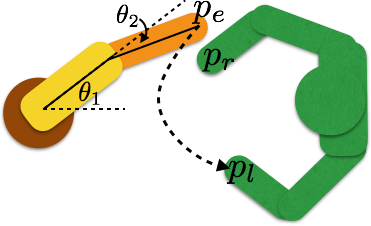
Figure 3: Human-robot co-operation: One example.

The design of the internal cost is illustrated below through an example shown in Fig. 3, where the human accepts a workpiece from the robot arm using his left hand. The robot arm has two links with joint positions $\theta_{1}$ and $\theta_{2}$ and the joint velocities $\dot{\theta}_{1}$ and $\dot{\theta}_{2}$. The configuration of the robot is $\theta=[\theta_{1},\theta_{2}]^{T}$. Considering the kinematics of the robot arm, the state is defined as $x_{R}=[\theta;\dot{\theta}]$ and the control input is defined to be the joint accelerations $u_{R}=\ddot{\theta}$. Then the dynamic equation satisfies,

$$f(x_{R})=\left[\begin{tabular}[]{cc}$0$&$I_{2}$\\ $0$&$0$\end{tabular}\right]x_{R},~{}g(x_{R})=\left[\begin{tabular}[]{c}$0$\\ $I_{2}$\end{tabular}\right].$$ (11)

Due to joint limits, the state constraint is $\Gamma:=\{x_{R}:\theta_{1}\in[-2\pi/3,2\pi/3],\theta_{2}\in[-\pi/2,\pi/2]\}$.

The area occupied by the robot arm is denoted as $\mathcal{C}(\theta)$. Denote the position of the human’s left hand as $p_{l}$ and the position of the human’s right hand as $p_{r}$. Then the human state is $x_{H}=[p_{l};p_{r};\dot{p}_{l};\dot{p}_{r}]$, which can be predicted by (6). The inverse kinematic function from the robot endpoint to the robot joint is denoted as $\mathcal{D}$. The cost function in (5a) is then designed as

$$J_{R}=\int_{0}^{T}(\|\theta(t)-\mathcal{D}(p_{l}(t))\|^{2}+\|u_{R}(t)\|^{2})dt,$$ (12)

which penalizes the distance from the robot end point to the human’s left hand. The look-ahead horizon $T$ can either be chosen as a fixed number or as a decision variable that should be optimized up to the accomplishment of the task. The interactive constraint in (5d) is designed as

$${X}_{S}(t)=\{x(t):\min_{p\in\mathcal{C}(\theta(t))}\|p_{r}(t)-p\|\geq d_{min}\},$$ (13)

where $d_{min}>0$ is the minimum required distance. For simplicity, the robot only avoids the human’s right hand in this formulation. This example will be re-visited in the following discussions.

III-C Logic: The Parallel Motion Planning

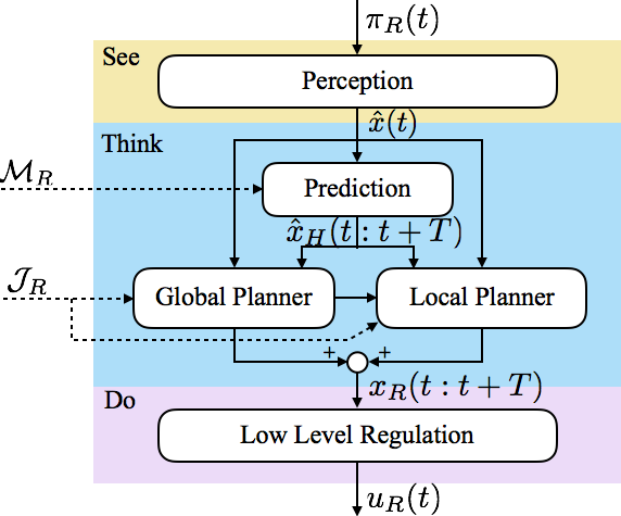
Figure 4: The designed architecture of the logic in the RSIS.

A “see-think-do” structure shown in Fig. 4 is adopted to tackle the complicated optimization problem (5). The mission of the “see” step is to process the high dimensional data $\pi_{R}(t)$ to obtain an estimate of the system state $\hat{x}(t)$. The “think” step is to solve (5) using the estimated states, and construct a realizable plan $x_{R}(t:t+T)$. The “do” step is to realize the plan by generating a control input $u_{R}(t)$.

In the “think” step, two important modules are prediction and planning. In the prediction module, robot $R$ makes predictions of other agents $\hat{x}_{H}(t:t+T)$ based on the internal model $\mathcal{M}_{R}$. The prediction can be a fixed trajectory or a function depending on robot $R$’s future state $x_{R}(t:t+T)$. In the planning module, the future movement $x_{R}(t:t+T)$ is computed given the current state $\hat{x}(t)$, predictions of others’ motion $\hat{x}_{H}(t:t+T)$ as well as the task requirements and constraints encoded in $\mathcal{J}_{R}$.

As it is computationally expensive to obtain the optimal solution of (5) for all scenarios in the design phase, the optimization problem is computed in the execution phase given real time measurements. However, there are two major challenges in real time motion planning. The first challenge is the difficulty in planning a safe and efficient trajectory when there are large uncertainties in other agents’ behaviors. As the uncertainty accumulates, solving the problem (5) in the long term might make the robot’s motion very conservative. The second challenge is real-time computation with limited computation power since problem (5) is highly non-convex. We design a unique parallel planning and control architecture to address the first challenge as will be discussed below, and develop fast online optimization solvers to address the second challenge as will be discussed in the Sections IV and V.

The parallel planner consists of a global (long term) planner as well as a local (short term) planner to address the first challenge by leveraging the benefits of the two planners. The idea is to have a long term planner solving (5) while considering only rough estimation of human’s future trajectory, and have a short term planner addressing uncertainties and enforcing the safety constraint (5d). The long term planning is efficiency-oriented and can be understood as deliberate thinking, while the short term planning is safety-oriented and can be understood as a reflex behavior.

The idea is illustrated in Fig. 5a. There is a closed environment. The robot (the purple dot) is required to approach the target (the green dot) while avoiding the human (the pink dot). The time axis is introduced to illustrate the spatiotemporal trajectories. For the long term planning, the robot has a rough estimation of the human’s trajectory and it plans a trajectory without considering the uncertainties in the prediction. Then the trajectory is used as a reference in the short term planning. In the first time step, the robot predicts the human motion (with uncertainty estimation) and checks whether it is safe to execute the long term trajectory. As the trajectory does dot intersect with the uncertainty cone, it is executed. In the next time step, since the trajectory is no longer safe, the short term planner modifies the trajectory by detouring. Meanwhile, the long term planner comes with another long term plan and the previous plan is overwrote. The short term planner then monitors the new reference trajectory. The robot follows the trajectory and finally approaches the goal. This approach addresses the uncertainty and is non conservative. As a long term planning module is included, it avoids the local optima problem that short term planners have.

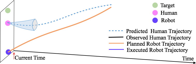
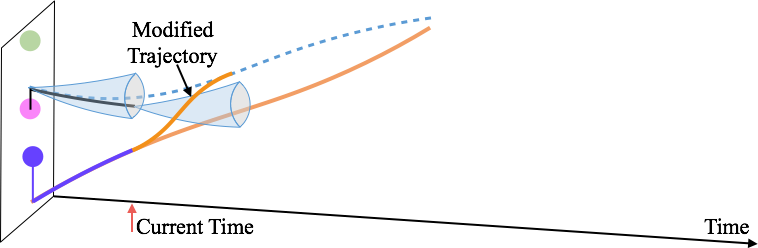
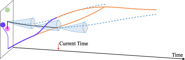
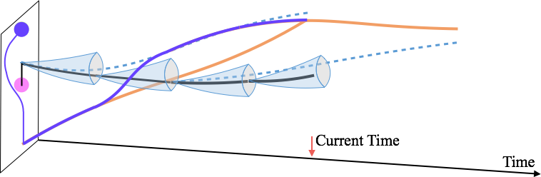
(a) Illustration of the performance.

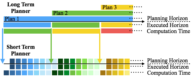
(b) Time flow of planning, execution, and computation.

Figure 5: Parallel planning.

The block diagram of the parallel controller architecture is shown in Fig. 4. In the following discussions, we also call the long term module as the efficiency controller and the short term module as the safety controller. This approach can be regarded as a two-layer MPC approach. The computation time flow is shown in Fig. 5b together with the planning horizon and the execution horizon. Three long term plans are shown, each with one distinct color. The upper part of the time axis shows the planning horizon. The middle layer is the execution horizon. The bottom layer shows the computation time. Once computed, a long term plan is sent to the short term planner for monitoring. The mechanism in the short term planner is similar to that in the long term planner. The planning horizon, the executed horizon and the computation time for the same short term plan are shown in the same color. The sampling rate in the short term planner is much higher than that in the long term planner, since a short term plan can be computed with shorter time. In this way, the uncertainty in the short term is much smaller than it could accumulate in the long term. The planning horizon in the short term planner is not necessarily one time step, though the execution horizon is one time step.

Coordination between the two layers is important. To avoid instability, a margin is added in the safety constraint in the long term planner so that the long term plan will not be revoked by the short term planner if the long term prediction of the human motion is correct. Theoretical analysis of the stability of the two-layer MPC method is out of the scope of this paper, and is left as a topic for future study. Nonetheless, successful implementation of the parallel architecture depends on computation. It is important that the optimization algorithms find feasible and safe trajectories within the sampling time. The algorithms will be discussed in Sections IV and V.

III-D Learning on the Model

The internal model $\mathcal{M}_{R}$ needs to be obtained from the learning process. Regarding (6), this paper adopts a feature-based reactive model,

$$\dot{x}_{H} = \sum_{j}a_{j}\varphi_{j}(x),$$ (14)

where $\varphi_{j}(x)$ are features such as distance to the robot, $a_{j}\in\mathbb{R}$ are coefficients that can be adapted online using recursive least square parameter identification (RLS-PAA) method [24, 26]. Moreover, it is assumed that $\dot{x}_{H}$ is bounded, since the maximum speed and acceleration of human are bounded.

IV The Safety-Oriented Short Term Planning

This section discusses how we use local planning to address safety. Suppose a reference input $u_{R}^{o}$ is received from the long term planner, the short term planner needs to ensure that the interaction constraint $x\in{X}_{S}$ will be satisfied after applying this input. Assuming $\Omega=\{u_{R}:|u_{R}|\leq\bar{u}_{R}\}$. The problem can be formulated as the following optimization,

$$u_{R}^{*}=~{} \min_{u_{R}}\|u_{R}-u_{R}^{o}\|^{2}_{Q},$$ (15a)

$$s.t.~{} u_{R}\in\Omega,x_{R}\in\Gamma,\dot{x}_{R}=f(x_{R})+h(x_{R})u_{R},$$ (15b)

$$x\in{X}_{S},$$ (15c)

where $\|u_{R}-u_{R}^{o}\|_{Q}=(u_{R}-u_{R}^{o})^{T}Q(u_{R}-u_{R}^{o})$ penalizes the deviation from the reference input, where $Q$ should be designed as a second order approximation of $J_{R}$, e.g. $Q\approx d^{2}J_{R}/d(u_{R})^{2}$. The constraints are the same as the constraints in (5). Note that modifying the control input is equivalent to modifying the trajectory as illustrated in Fig. 5a. In this section, we call $X_{S}$ the safe set. Without loss of generality, it is assumed that $x\in X_{S}$ implies that $x_{R}\in\Gamma$. Otherwise, we just take the intersection of the two constraints. The safe set and the robot dynamics impose nonlinear and non-convex constraints which make the problem hard to solve. We then transform the non-convex state space constraint into convex control space constraint using the idea of invariant set. Code is available github.com/changliuliu/SafeSetAlgorithm.

IV-A The Safety Principle

Suppose the estimate of human state is $\hat{x}_{H}$ and the uncertainty range is $\Gamma_{H}$. According to the safe set $X_{S}$, define the state space constraint $R_{S}$ for the robot to be

$$R_{S}= \{x_{R}:[x_{R};x_{H}]\in X_{S},\forall x_{H}\in\Gamma_{H}\}.$$ (16a)

The safety principle specifies that the robot control input $u_{R}(t)$ should be chosen such that $X_{S}$ is invariant, i.e. $x(t)\in X_{S}$ for all $t$, or equivalently, $x_{R}(t)\in R_{S}(t)$ for $\Gamma_{H}(t)$ which accounts for almost all possible noises $v_{1},...v_{N},w_{1},...,w_{N}$ and human behaviors $\mathcal{B}_{i}(\cdot),i\in H$ (those with negligible probabilities will be ignored).

Figure 6: Illustration of the safe set $X_{S}$ and the safety index $\phi$.

IV-B The Safety Index

The safety principle requires the designed control input to make the safe set invariant with respect to time. In addition to constraining the motion in the safe region $R_{S}$, the robot should also be able to cope with any unsafe human movement. To cope with the safety issue dynamically, a safety index is introduced as shown in Fig. 6. The safety index $\phi:X\rightarrow\mathbb{R}$ is a function on the system state space such that 1) $\phi$ is differentiable with respect to $t$, i.e. $\dot{\phi}=(\partial\phi/\partial x)\dot{x}$ exists everywhere; 2) $\partial{\dot{\phi}}/\partial{u_{R}}\neq 0$; 3) The unsafe set $X\setminus X_{S}$ is not reachable given the control law $\dot{\phi}<0\left.when\right.\phi\geq 0$ and the initial condition $x(t_{0})\in X_{S}$.

The first condition is to ensure that $\phi$ is smooth. The second condition is to ensure that the robot input can always affect the safety index. The third condition provides a criteria to determine whether a control input is safe or not, e.g., all the control inputs that drive the state below the level set $0$ are safe and unsafe otherwise. The construction of such an index is discussed in [23]. Applying such a control law will ensure the invariance of the safe set, hence guarantee the safety principle. To consider the constraints on control, we need to further require that $\min_{u_{R}\in\Omega}\dot{\phi}<0$ for $\phi=0$ given that the human movement $\dot{x}_{H}$ is bounded.

IV-C The Set of Safe Control

To ensure safety, the robot’s control must be chosen from the set of safe control $U_{S}(t)=\{u_{R}(t):\dot{\phi}\leq-\eta_{R}\left.when\right.\phi\geq 0\}$ where $\eta_{R}\in\mathbb{R}^{+}$ is a safety margin. By the dynamic equation in (15b), the derivative of the safety index can be written as $\dot{\phi}=\frac{\partial\phi}{\partial x_{R}}hu_{R}+\frac{\partial\phi}{\partial x_{R}}f+\frac{\partial\phi}{\partial x_{H}}\dot{x}_{H}$. Then

$$U_{S}\left(t\right)=\left\{u_{R}\left(t\right):L\left(t\right)u_{R}\left(t\right)\leq\min_{\dot{x}_{H}\in\dot{\Gamma}_{H}}S\left(t,\dot{x}_{H}\right)\right\},$$ (17)

where $\dot{\Gamma}_{H}$ is the set of velocity vectors that move $x_{H}$ to $\Gamma_{H}$, which can be obtained by estimating the mean squared error in the learning model [25],

$$L\left(t\right)= \frac{\partial\phi}{\partial x_{R}}h,$$ (18a)

$$S\left(t,\dot{x}_{H}\right)= \begin{cases}\begin{array}[]{c}-\eta_{R}-\frac{\partial\phi}{\partial x_{H}}\dot{x}_{H}-\frac{\partial\phi}{\partial x_{R}}f\\ \infty\\ \end{array}\begin{array}[]{c}\phi\geq 0\\ \phi<0\\ \end{array}\end{cases}.$$ (18b)

$L(t)$ is a vector at the “safe” direction, while $S(t,\dot{x}_{H})$ is a scalar indicating the allowed range of safe control input, which can be broken down into three parts: a margin $-\eta_{R}$, a term to compensate human motion $-\frac{\partial\phi}{\partial x_{H}}\dot{x}_{H}$ and a term to compensate the inertia of the robot itself $-\frac{\partial\phi}{\partial x_{R}}f_{R}$. In the following discussion when there is no ambiguity, $S(t,\dot{x}_{H})$ denotes the value in the case $\phi\geq 0$ only.

The difference between $R_{S}$ and $U_{S}$ is that $R_{S}$ is static as it is on the state space, while $U_{S}$ is dynamic as it concerns with the “movements”. Due to introduction of the safety index, the non-convex state space constraint $R_{S}$ is transformed to a convex control space constraint $U_{S}$. Since $\Omega$ is usually convex, the problem (15) is transformed to a convex optimization,

$$u_{R}^{*}=~{} \min\|u_{R}-u_{R}^{o}\|^{2}_{Q},$$ (19a)

$$s.t.~{} u_{R}\in\Omega\cap U_{S}.$$ (19b)

The switch condition in (18b) may result in oscillation for discrete time implementation. A smoothed version of the algorithm is discussed in [19].

IV-D Example: Safe control on a planar robot arm

In this part, the design of the safety index and the computation of $U_{S}$ with respect to (13) will be illustrated on the planar robot arm shown in Fig. 3. The closest point to $p_{r}$ on the robot arm is denoted as $c\in\mathbb{R}^{2}$. The distance is denoted as $d=\|c-p_{r}\|$. The relationship among $\dot{c}$, $\ddot{c}$, $x_{R}=[\theta;\dot{\theta}]$ and $u_{R}=\ddot{\theta}$ is

$$\dot{c}=J_{c}\dot{\theta},~{}~{}\ddot{c}=J_{c}u_{R}+H_{c},$$

where $J_{c}$ is the Jacobian matrix at $c$ and $H_{c}=\dot{J_{c}}\dot{\theta}$. The constraint in (13) requires that $d\geq d_{min}$. Since the order from $c$ to $u_{R}$ in the Lie derivative sense is two, the safety index is designed to include the first order derivative of $d$ in order to ensure that $\partial\dot{\phi}/\partial u_{R}\neq 0$. The safety index is then designed as $\phi=D-d^{2}-k_{\phi}\dot{d}$. The parameters $D>d_{min}^{2}$ and $k_{\phi}>0$ are chosen such that $\min_{|u_{R}|\leq\bar{u}_{R}}\dot{\phi}<0$ for $\phi=0$ and $c$ being the robot end point. In addition to $\dot{p}_{r}$ and $\ddot{p}_{r}$ being bounded, $p_{r}$ is also assumed to be bounded as the human hand is not allowed to get close to the robot base. Moreover, the robot is not allowed to go to the singular point. For such $\phi$, it is easy to verify that the conditions specified above are all satisfied [23]. Now we compute the constraint on the control space. Let the relative distance, velocity and acceleration vectors be $\mathbf{d}=c-p_{r}$,$\mathbf{v}=\dot{c}-\dot{p}_{r}$ and $\mathbf{a}=\ddot{c}-\ddot{p}_{r}$. Then $d=|\mathbf{d}|$ and

$$\dot{\phi}= -2d\dot{d}-k_{\phi}\ddot{d}=-2\mathbf{d}^{T}\mathbf{v}-k_{\phi}\frac{\mathbf{d}^{T}\mathbf{a}+\mathbf{v}^{T}\mathbf{v}-\dot{d}^{2}}{d},$$

$$= -2\mathbf{d}^{T}\mathbf{v}-k_{\phi}\frac{\mathbf{d}^{T}\left(J_{c}u_{R}+H_{c}-\ddot{p}_{r}\right)+\mathbf{v}^{T}\mathbf{v}-\frac{(\mathbf{d}^{T}\mathbf{v})^{2}}{d^{2}}}{d}.$$

Hence the parameters in (17) are

$$L(t)= -k_{\phi}\frac{\mathbf{d}^{T}}{d}J_{c},$$

$$S(t)= -\eta_{R}+2\mathbf{d}^{T}\mathbf{v}+k_{\phi}\frac{\mathbf{d}^{T}H_{c}-\mathbf{d}^{T}\ddot{p}_{r}+\mathbf{v}^{T}\mathbf{v}-\frac{(\mathbf{d}^{T}\mathbf{v})^{2}}{d^{2}}}{d}.$$

Then $U_{S}$ can be obtained given the uncertainty on human motion $\ddot{p}_{r}$.

V Efficiency-Oriented Long Term Planning

To avoid local optima in short term planning, long term planning is necessary. However, the optimization problem (5) in a clustered environment is usually highly nonlinear and non-convex, which is hard to solve in real time using generic non-convex optimization solvers such as sequential quadratic programming (SQP) [3] and interior point method (ITP) [33] that neglect the unique geometric features of the problem. CFS [21] has been proposed to convexify the problem considering the geometric features for fast real time computation. This section further assumes that the cost function is convex with respect to the robot state and control input, and the system dynamics are linear. A method to convexify a problem with nonlinear dynamic constraints is discussed in [27]. CFS code is available github.com/changliuliu/CFS.

V-A Long Term Planning Problem

Discretize the robot trajectory into $h$ points and define $x_{R}^{q}:=x_{R}(qt_{s}+t_{0})$ where $t_{0}$ is the current time, $t_{s}$ is the sampling time. The discrete trajectory is denoted $\mathbf{x}_{R}:=[x_{R}^{0};x_{R}^{1};\ldots;x_{R}^{h}]$. Similarly, the trajectory of the control input is $\mathbf{u}_{R}:=[u_{R}^{0};u_{R}^{1};\ldots;u_{R}^{h-1}]$. The predicted human trajectory is denoted $\hat{\mathbf{x}}_{H}:=[\hat{x}_{H}^{0};\hat{x}_{H}^{1};\ldots;\hat{x}_{H}^{h}]$. It is assumed that the system dynamics are linear and observable. Hence $\mathbf{u}_{R}$ can be computed from $\mathbf{x}_{R}$, i.e. $\mathbf{u}_{R}=\mathcal{L}(\mathbf{x}_{R})$ for some linear mapping $\mathcal{L}$. Rewriting (5) in the discrete time as

$$\min_{\mathbf{x}_{R}\in\Gamma^{e}}~{}J_{R}^{d}(\mathbf{x}_{R})$$ (22)

where $J_{R}^{d}(\mathbf{x}_{R})$ is the discretized cost function, and $\Gamma^{e}:=\{\mathbf{x}_{R}:\mathcal{L}(\mathbf{x}_{R})\in\oplus_{h}\Omega,x_{R}^{q}\in\Gamma,[x_{R}^{q};\hat{x}_{H}^{q}]\in{X}_{S}\}$. The symbol $\oplus$ is for direct sum, which is taken since $\mathbf{u}_{R}=\mathcal{L}(\mathbf{x}_{R})$ has $h$ components and each belongs to $\Omega$. Since $J_{R}$ is convex and $\mathbf{u}_{R}$ depends linearly on $\mathbf{x}_{R}$, $J_{R}^{d}$ is also convex. The non-convexity mainly comes from the constraint $\Gamma^{e}$.

V-B Convex Feasible Set Algorithm

To make the computation more efficient, we transforms (22) into a sequence of convex optimizations by obtaining a sequence of convex feasible sets inside the non-convex domain $\Gamma^{e}$. The general method in constructing convex feasible set is discussed in [21]. In this paper, we assume that $\Omega$ and $\Gamma$ are convex. The only constraint that needs to be convexified is the interactive constraint $[x_{R}^{q};\hat{x}_{H}^{q}]\in{X}_{S}$. For each time step $q$, the infeasible set in the robot’s state space is $\mathcal{O}_{q}:=\{x_{R}^{q}:[x_{R}^{q};\hat{x}_{H}^{q}]\notin{X}_{S}\}$. Then the interactive constraint in (22) is equivalent to $d^{*}(x_{R}^{q},\mathcal{O}_{q})\geq 0$ where $d^{*}(x_{R}^{q},\mathcal{O}_{q})$ is the signed distance function to $\mathcal{O}_{q}$ such that

$$d^{*}(x_{R}^{q},\mathcal{O}_{q}):=\left\{\begin{array}[]{cc}\min_{z\in\partial\mathcal{O}_{q}}\|x_{R}^{q}-z\|&x_{R}^{q}\notin\mathcal{O}_{q}\\ -\min_{z\in\partial\mathcal{O}_{q}}\|x_{R}^{q}-z\|&x_{R}^{q}\in\mathcal{O}_{q}\end{array}\right..$$ (25)

The symbol $\partial\mathcal{O}_{q}$ denotes the boundary of the obstacle $\mathcal{O}_{q}$.

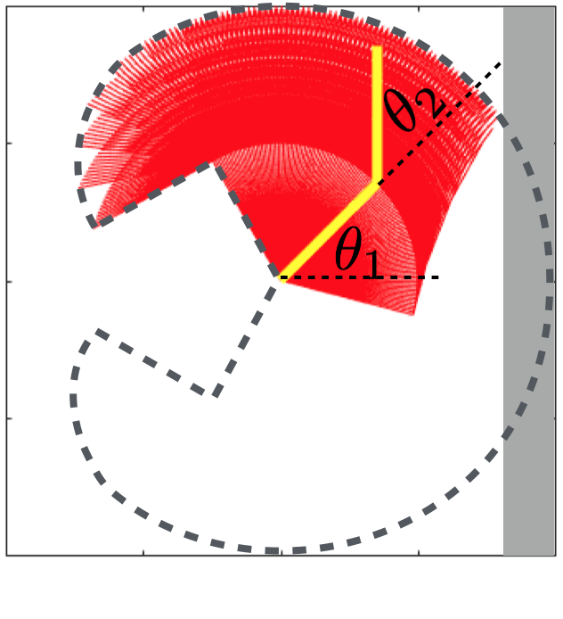
(a) Cartesian space.

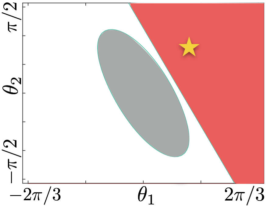
(b) Configuration space.

Figure 7: Illustration of the constraint and the convex feasible set for a planar robot arm in Cartesian and Configuration spaces.

If $\mathcal{O}_{q}$ is convex, then the function $d^{*}(\cdot,\mathcal{O}_{q})$ is also convex. Hence $d^{*}(x_{R}^{q},\mathcal{O}_{q})\geq d^{*}(r^{q},\mathcal{O}_{q})+\nabla d^{*}(r^{q},\mathcal{O}_{q})(x_{R}^{q}-r^{q})$ for any reference point $r^{q}$. Then $d^{*}(r^{q},\mathcal{O}_{q})+\nabla d^{*}(r^{q},\mathcal{O}_{q})(x_{R}^{q}-r^{q})\geq 0$ implies that $x_{R}^{q}\notin\mathcal{O}_{q}$. If the obstacle $\mathcal{O}_{q}$ is not convex, we then break it into several simple overlapping convex objects $\mathcal{O}^{i}_{q}$ such as circles or spheres, polygons or polytopes. Then $d^{*}(\cdot,\mathcal{O}^{i}_{q})$ is the convex cone of the convex set $\mathcal{O}_{q}^{i}$. Suppose the reference trajectory is $\mathbf{r}:=[r^{0};r^{1};\ldots;r^{h}]$, the convex feasible set $\mathcal{F}(\mathbf{r})$ for (22) is defined as

$$\mathcal{F}(\mathbf{r}):=\{\mathbf{x}_{R}:\mathcal{L}(\mathbf{x}_{R})\in\oplus_{h}\Omega,x_{R}^{q}\in\Gamma,$$ (26a)

$$~{}~{}~{}~{}d^{*}(r^{q},\mathcal{O}_{q}^{i})+\nabla d^{*}(r^{q},\mathcal{O}_{q}^{i})(x_{R}^{q}-r^{q})\geq 0,\forall q,i\},$$ (26b)

which is a convex subset of $\Gamma^{e}$.

Starting from an initial reference trajectory $\mathbf{x}_{R}^{(0)}$, the convex optimization (27) needs to be solved iteratively until either the solution converges or the descent of cost $J_{R}^{d}$ is small.

$$\mathbf{x}_{R}^{(k+1)}=\arg\min_{\mathbf{x}_{R}\in\mathcal{F}(\mathbf{x}_{R}^{(k)})}J_{R}^{d}(\mathbf{x}_{R}).$$ (27)

It has been proved in [21] that the sequence $\{\mathbf{x}_{R}^{(k)}\}$ converges to a local optimum of problem (22). Moreover, the computation time can be greatly reduced using CFS. This is due to the fact that we directly search for solutions in the feasible area. Hence 1) the computation time per iteration is smaller than existing methods as no linear search is needed, and 2) the number of iterations is reduced as the step size (change of the trajectories between two consecutive steps) is unconstrained.

V-C Example: Long term planning for a planar robot arm

The previous example in Fig. 3 is considered. Let $T=ht_{s}$. Then the discretized optimization problem is formulated as

$$\min_{\boldsymbol{\theta}}~{} \sum_{q}\|\theta^{q}-\mathcal{D}(p_{l}^{q})\|+\|\frac{{\theta}^{q+1}-2{\theta}^{q}+{\theta}^{q-1}}{t_{s}^{2}}\|,$$ (28a)

$$s.t.~{} \theta_{1}^{q}\in[-2\pi/3,2\pi/3],\theta_{2}^{q}\in[-\pi/2,\pi/2],$$ (28b)

$$\|p_{r}^{q}-p\|\geq d_{min},\forall p\in\mathcal{C}(\theta^{q}),\forall q,$$ (28c)

where $\boldsymbol{\theta}=[\theta^{0};\ldots;\theta^{h}]$, (28a) is the discrete version of (12) and (28c) is the discrete version of (13). The control input $\ddot{\theta}$ is computed using finite difference. The constraint (28c) is in the Cartesian space $\mathbb{R}^{2}$, which needs to be transformed into the configuration space $[-\pi,\pi)\times[-\pi,\pi)$. For example, suppose that the base of the robot arm is at the origin; the links of the robot are of unit length; and the constraint (28c) requires that the robot arm is outside of the danger zone $x\geq 1.7$, i.e. $[0~{}1]p\leq 1.7$. The danger zone is shown in gray in Fig. 7a. Then the constraint in the configuration space is $\cos\theta_{1}+\cos(\theta_{1}+\theta_{2})\leq 1.7$ where the danger zone is transformed into a convex ellipsoid-like object as shown in Fig. 7b. Consider a reference point $(\pi/4,\pi/4)$, the convex feasible set in the configuration space is computed as $\cos(\pi/4)+\cos(\pi/2)-\sin(\pi/4)(\theta_{1}-\pi/4)-\sin(\pi/2)(\theta_{1}+\theta_{2}-\pi/2)=\sqrt{2}/{2}-\sqrt{2}/{2}(\theta_{1}-\pi/4)-(\theta_{1}+\theta_{2}-\pi/2)\leq 1.7$, which is illustrated in the red area in Fig. 7b. Note that we did not use a distance function to convexify the obstacle, since the function $\cos\theta_{1}+\cos(\theta_{1}+\theta_{2})$ is already convex in the domain (28b). The area occupied by the robot given the configuration in the convex feasible set is illustrated in red in Fig. 7a. The dashed curve denotes the reachable area of the robot arm given the constraint (28b). The constraint (28c) can be convexified for every step $q$. Then the discrete long term problem (28) can be solved efficiently by iteratively solving a sequence of quadratic programs.

VI Evaluation Platforms

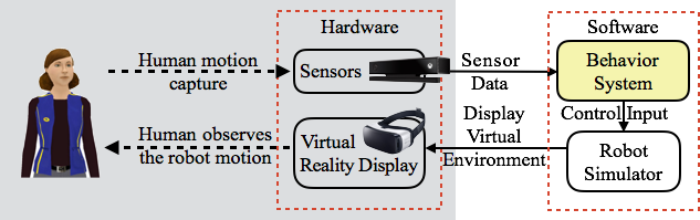
(a) Virtual reality-based human-in-the-loop platform.

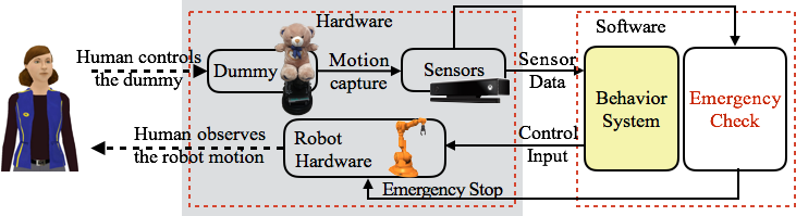
(b) Dummy-robot interaction platform.

Figure 8: The evaluation platforms.

To evaluate the performance of the designed behavior system, pure simulation is not enough. However, to protect human subjects, it is desired that we separate human subjects and robots physically during the early phase of deployment. This section introduces two evaluation platforms that we developed to evaluate the designed behavior system, as shown in Fig. 8.

VI-A A Human-in-the-loop Simulation Platform

The platform in Fig. 8a is a virtual reality-based human-in-the-loop platform. The robot’s motion is simulated in the robot simulator. A human subject observes the robot movement through the virtual reality display (e.g. virtual reality glasses, augmented reality glasses or monitors). The reaction of the human subject is captured by sensors (e.g. Kinect or touchpad). The sensor data is sent to the behavior system to compute desired control input. The advantage of such platform is that it is safe to human subjects and convenient for idea testing. The disadvantage is that the robot simulator may neglect dynamic details of the physical robot, hence may not be reliable. Nonetheless, the human data obtained in such platform can be stored for offline analysis in order to let the robot build better cognitive models.

One human-in-the-loop simulation platform for industrial robot is illustrated in Fig. 9a. The left of the figure shows the human subject whose motion is captured by a Kinect. The right of the figure shows the virtual environment displayed on a screen. The robot links are replaces with capsules, while the human is displayed as skeletons. The task for the robot is relatively simple in this platform, e.g. to hold the neutral position or to follow a simple trajectory. The only hardware requirement is a computer, a Kinect and a monitor. The software package is available github.com/changliuliu/VRsim.

VI-B A Dummy-Robot Interaction Platform

The platform in Fig. 8b is a dummy-robot interaction platform. The interaction happens physically between the dummy and the robot. The human directly observes the robot motion and controls the dummy to interact with the robot. As there are physical interactions, an emergency check module is added to ensure safety. The advantage of such platform is that it is safe to human subjects, while it is able to test interactions physically. However, the disadvantage is that the dummy usually doesn’t have as many degrees of freedom as a human subject does.

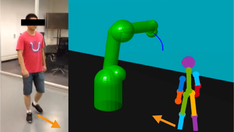
(a) Human-in-the-loop simulation platform.

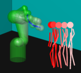
(b) Time step 20:5:40

(c) Time step 100:5:120

Figure 9: The human-in-the-loop simulation.

One dummy-robot platform is shown in Fig. 11a, where the robot is performing a pick-and-place task. There is a 6 degree of freedom industrial robot arm (FANUC LR Mate 200iD/7L) with gripper, a Kinect for environment monitoring, a workpiece, a target box and an obstacle. The environment perceived by the robot is visualized on a screen. The status of the robot is shown in the monitor. The robot needs to pick the workpiece and place it in the target box while avoiding the dynamic obstacle. The scenario can be viewed as a variation of the human-robot cooperation in Fig. 3, where the green target box represents the human’s left hand that accepts the workpiece from the robot, and the red box represents the human’s right hand that needs to be avoided. The positions of the boxes can be controlled by human subjects at a distance to the robot arm.

VII Experiment Results

VII-A The Human-in-the-loop Platform

Figure 10: The result in the human-in-the-loop simulation

The experiment with the human-in-the-loop platform was run on a MacBook Pro with 2.3 GHz Intel Core i7. The robot arm is required to stay in the neutral position while maintaining a minimum distance $d_{min}=0.2m$ to the human. The sampling time is $t_{s}=0.1s$. The human state $x_{H}$ is taken as the skeleton position of the human subject. The uncertainty of human movement is bounded by a predefined maximum speed of the human subject. More accurate prediction models are discussed in [22]. The robot in the simulation has six degree of freedoms. Its control input is the joint acceleration $\ddot{\theta}$. Since the robot is not performing any task, a stabilizing controller that keeps the robot arm at the neutral position is adopted instead of a long term planner. Collision avoidance is taken care of by the short term safety controller, which implements the safe set algorithm discussed in Section IV. The safety index is the same as the one in Section IV-D, which depends not only on the relative distance but also the relative velocity.

The performance of the safety controller is shown in Fig. 10, where the first graph shows the deviations of the joint positions from the neutral position, followed by a graph of the minimum distance between the human and the robot, and a graph of the activity of the safety controller. The horizontal axis is the time axis. In the distance profile, the solid curve is the true distance, while the dashed curve shows the distance in the case that the robot does not turn on the safety controller. Without the safety controller, the distance profile enters the danger zone ($d<d_{min}$) between time step 30 and 110. With the safety controller, the distance profile is always maintained above the danger zone. Moreover, as the dangerous situation is anticipated in advance, a modification signal is generated as early as at time step 22. The scenario at time step 20 to 40 is shown in Fig. 9b where the snapshots are taken every 5 time steps. The lighter the color, the earlier it is in time. The blue curve is the trajectory of the robot end point. As the robot anticipates that the human will come closer, it moves backward. The scenario at time step 100 to 120 is shown in Fig. 9c. As the robot anticipates that the human will go away, it returns to the neutral position. The safety controller is active between time step 20 to 120, which roughly aligns with the moments that the distance between the human and the robot in the neutral position is smaller than $d_{min}$. When the safety controller is active, all joint positions are affected.

The algorithm is run in Matlab script. The average computation time in solving (19) is 0.4ms, while the average time in obtaining $U_{S}^{3}$ is 3.9ms, where the computation of the distance $d$ takes the majority of the time. Nonetheless, the total computation time is still small enough for real time human robot interactions. Moreover, when compiled in C in the dummy-robot platform, the computation time can be kept lower than 1ms.

VII-B The Dummy-Robot Platform

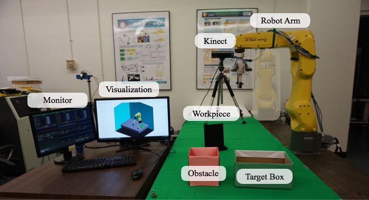
(a) The platform.

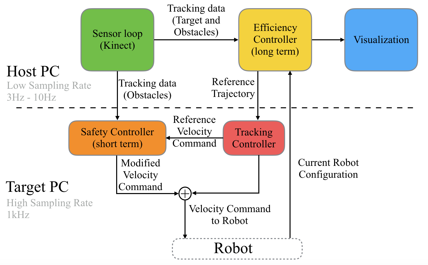
(b) RSIS software architecture.

Figure 11: The dummy-robot platform for industrial robot.

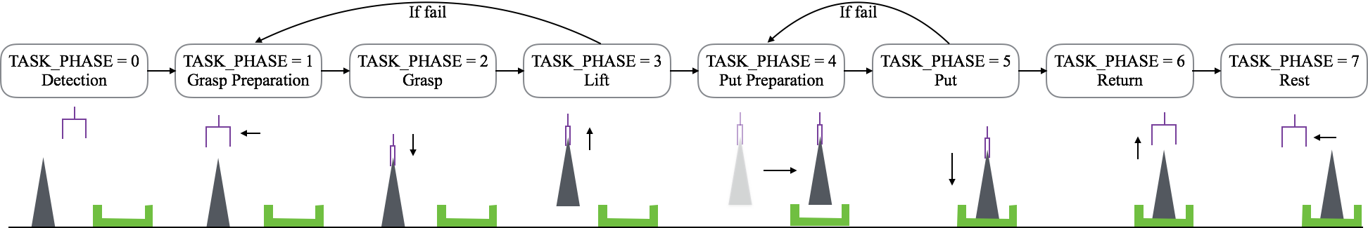
Figure 12: Finite state machine for the pick-and-place task.

In the dummy-robot platform, the software implementation of the architecture in Fig. 4 is shown in Fig. 11b. There are two PCs in the system. Algorithms that require longer computation time are implemented on the host PC, while algorithms that compute faster are implemented on the target PC. The target PC runs Simulink RealTime with Intel i5-3340 Quad-Core CPU 3.10 GHz. Communications between the host PC and the target PC are enabled by user datagram protocol (UDP).

There are five modules in the implementation: sensor loop, efficiency controller, visualization, safety controller and tracking controller.

Host PC

On host PC, sensor loop takes care of the perception and prediction in Fig. 4, which measures the state of the objects and predicts their future trajectories. In this platform, the trajectories of the objects are predicted assuming constant speed. The objects are attached with ARTags [8] for detection (now shown in the figure). The efficiency controller implements CFS to solve the following optimization problem,

$$\min_{\boldsymbol{\theta}}~{}~{} J(\boldsymbol{\theta})=w_{1}\|\boldsymbol{\theta}-\mathbf{r}\|^{2}_{S}+w_{2}\|\boldsymbol{\theta}\|^{2}_{R}$$ (29a)

$$s.t.~{}~{} \theta^{0}=r^{0},\theta^{h}=r^{h},\underline{\theta}\leq\theta^{q}/t_{s}\leq\bar{\theta}$$ (29b)

$$\|p_{r}^{q}-p\|\geq d_{min},\forall p\in\mathcal{C}(\theta^{q}),\forall q,$$ (29c)

where $\boldsymbol{\theta}\in\mathbb{R}^{6(h+1)}$ is the discrete trajectory which consists of the joint positions of the robot in different time steps. The horizon $h$ is determined by the horizon of the reference trajectory $\mathbf{r}\in\mathbb{R}^{6(h+1)}$.

The reference trajectory is generated according to the current task phase as specified in the finite state machinein Fig. 12. Eight phases have been identified in the put-and-place task. In each phase, the ending pose will be estimated first. For example, by the end of the grasp preparation phase, the gripper should locate right above the workpiece. Then the time $T$ for the robot to go to the ending pose will be estimated assuming that the robot end point is moving at a constant speed. Then $h$ is set as $T/t_{s}$, $r^{0}$ in the reference trajectory as the current pose, and $r^{h}$ as the ending pose. The reference trajectory $\mathbf{r}$ is then obtained by linear interpolation between $r^{0}$ and $r^{h}$. In the constraint (29b), the boundary constraints are specified, and $\underline{\theta}$ and $\bar{\theta}$ are the lower and upper joint limits. The collision avoidance constraint is specified in (29c) where $p_{r}^{q}$ is the position of the obstacle at time step $q$ and $d_{min}\in\mathbb{R}^{+}$. To simplify the distance function, the robot geometry $\mathcal{C}(\theta^{q})$ is represented by several capsules as shown in Fig. 9a. When the robot is carrying the workpiece, the workpiece is also wrapped in the capsules. The minimum distance $d$ is then computed with respect to the centerlines of the capsules as discussed in [26].

The collision avoidance constraint (29c) can be convexified according to (26b) where the gradients are taken numerically. The optimization problem is then solved using CFS. The final trajectory is sent to the target PC as a reference trajectory.

Target PC

On target PC, a tracking controller is used to track the trajectory in order to account for delay, package loss, and sampling time mismatch between the two PCs. The safety controller monitors the trajectory. The safety index is the same as the one discussed in the example in Section IV. The uncertainty cone is bounded by the maximum acceleration of the object. Finally, a velocity command will be sent to a low level controller to move the robot. The algorithms in the host PC are run in Matlab script on the host PC, while the algorithms on the target PC are compiled into C.

Performance

The performance of the robot in one task scenario is shown in Fig. 13, where the left of every figure shows the perceived environment from the Kinect, while the right of every figure shows the real world scenario. The yellow curve is the planned long term trajectory. Though the trajectory is planned in the joint space, it is only shown for the robot end point for clarity. The obstacle is moving around causing disturbances to the robot arm. The robot generates detours to avoid the obstacle in TASK_PHASE 4 as shown in Fig. 13e and in TASK_PHASE 6 as shown in Fig. 13h. Sometimes the planned trajectory is perfectly followed as shown in Fig. 13f. Sometimes the trajectory is modified by the safety controller to avoid the obstacle as shown in Fig. 13d and 13i, since the obstacle’s state is not the same as predicted in the efficiency controller.

To reduce the computation time on the host PC, the planning horizon is limited to $h\leq 6$. For solving the optimization (29) in the efficiency controller, CFS takes 0.341s on average, while SQP takes 3.726s and ITP takes 2.384s. CFS is significantly faster than SQP and ITP. In CFS algorithm, 98.1% of the computation is used to convexify the problem and only 1.9% of the time is used to solve the resulting quadratic programming. The most time consuming operation in convexification is to take the numerical derivative. Hence if better method is developed, the computation time can be further reduced.

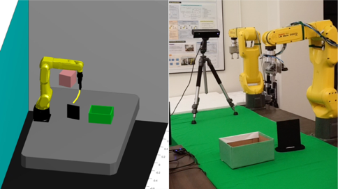
(a) TASK_PHASE = 1. $T=17s$.

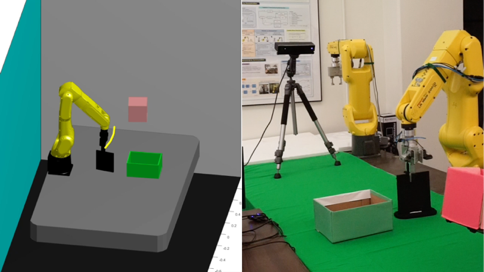
(b) TASK_PHASE = 2. $T=20s$.

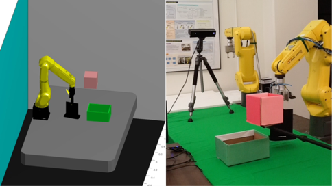
(c) TASK_PHASE = 3. $T=24s$.

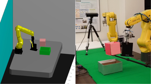
(d) TASK_PHASE = 3. $T=26s$.

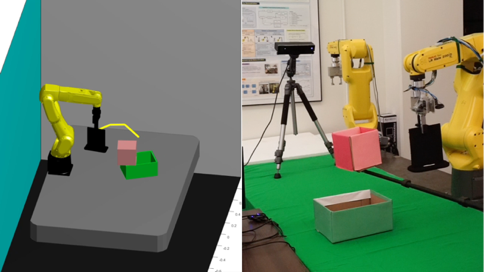
(e) TASK_PHASE = 4. $T=28s$.

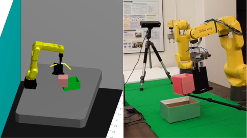
(f) TASK_PHASE = 4. $T=31s$.

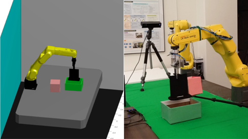
(g) TASK_PHASE = 5. $T=34s$.

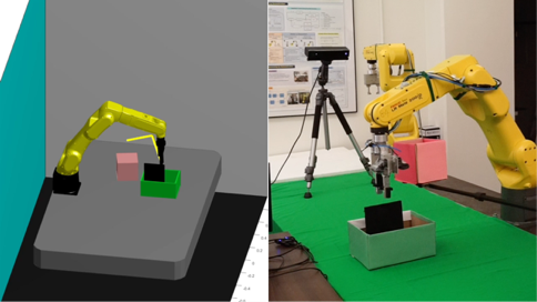
(h) TASK_PHASE = 6. $T=39s$.

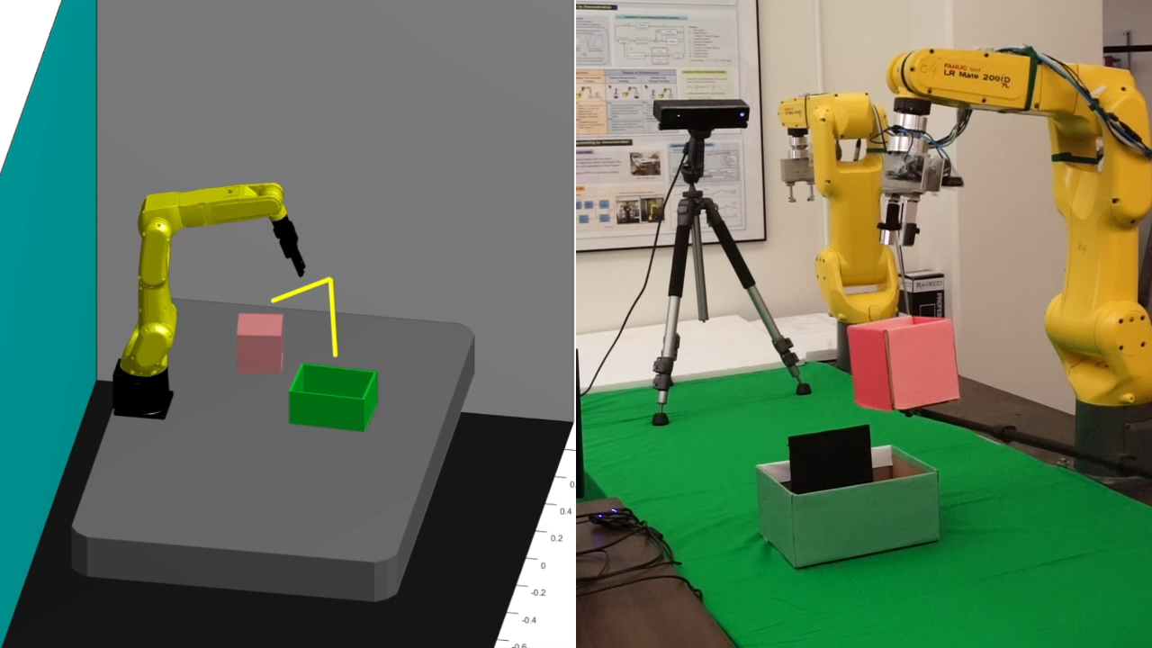
(i) TASK_PHASE = 7. $T=44s$.

Figure 13: The experiment result on the dummy-robot platform.

VIII Discussion

It has been verified that RSIS is capable of interacting safely and efficiently with humans. Nonetheless, there are many directions for future works.

To learn skills

When the complexity of tasks increases, it is hard to design knowledge, especially the internal cost (5) from scratch. It may be better for the robot to learn the skills directly from human demonstration [31].

To consider communication among agents

This paper only optimizes physical movements of robots to accomplish tasks. To better facilitate interactions, intentions could also be communicated among agents to avoid mis-understandings. Moreover, physical movements can be communicative as it reveals one’s intention to observers [7]. We will build such knowledge about communicative motions into the robot behavior system in the future.

To improve computation efficiency

Computation efficiency of the designed algorithms is extremely important. This paper adopts convexification methods to speed up the computation of non-convex optimization. However, several assumptions narrowed the scope of the proposed algorithms, which should be relaxed in the future.

To analyze the designed robot behavior

We provided experimental verification of the designed robot behavior. However, theoretical analysis and formal guarantee is important to provide a deep insight into the system properties and ways to improve the design. In theoretical analysis, the questions that need to be answered are: (1) Is the parallel planner stable and optimal? (2) Will the learning process converge to the true value? (3) Will the designed behavior help achieve system optima in the multi-agent system?

Based on RSIS, we recently developed safe and efficient robot collaboration system (SERoCS) [22], which further incorporates robust cognition algorithms for environment monitoring, and efficient task planning algorithms for reference generations. As a future work, we will also compare our methods with other methods [18] on our platforms for a variety of tasks that involve human-robot interactions.

IX Conclusion

This paper introduced the robot safe interaction system (RSIS) for safe real time human-robot interaction. First, a general framework concerning macroscopic multi-agent system and microscopic behavior system was discussed. The design of the behavior system was challenging due to uncertainties in the system and limited computation capacity. To equip the robot with a global perspective and ensure timely responses in emergencies, a parallel planning and control architecture was proposed, which consisted of an efficiency-oriented long term planner and a safety-oriented short term planner. The convex feasible set algorithm was adopted to speed up the computation in the long term motion planning. The safe set algorithm was adopted to guarantee safety in the short term. To protect human subjects in the early phase of deployment, two kinds of platforms to evaluate the designed behavior was proposed. The experiment results with the platforms verified the effectiveness and efficiency of the proposed method. Several future directions were pointed out in the discussion session and will be pursued in the future.

References

- [1] Working with robots: Our friends electric. The Economist, 2013.
- [2] T. M. Anandan. Major robot OEMs fast-tracking cobots, 2014.
- [3] P. T. Boggs and J. W. Tolle. Sequential quadratic programming. Acta numerica, 4:1–51, 1995.
- [4] C. Breazeal. Social interactions in hri: the robot view. IEEE Transactions on Systems, Man, and Cybernetics-Part C: Applications and Reviews, 34(2):181–186, 2004.
- [5] G. Charalambous. Human-automation collaboration in manufacturing: Identifying key implementation factors. In Proceedings of the International Conference on Ergonomics & Human Factors, page 59. CRC Press, 2013.
- [6] K. Dautenhahn. Socially intelligent robots: Dimensions of human–robot interaction. Philosophical Transactions of the Royal Society B: Biological Sciences, 362(1480):679–704, 2007.
- [7] A. Dragan. Legible Robot Motion Planning. PhD thesis, Carnegie Mellon University, 2015.
- [8] M. Fiala. ARTag, a fiducial marker system using digital techniques. In IEEE Conference on Computer Vision and Pattern Recognition (CVPR), volume 2, pages 590–596 vol. 2, June 2005.
- [9] T. Fong, I. Nourbakhsh, and K. Dautenhahn. A survey of socially interactive robots. Robotics and Autonomous Systems, 42(3):143–166, 2003.
- [10] E. Gribovskaya, A. Kheddar, and A. Billard. Motion learning and adaptive impedance for robot control during physical interaction with humans. In Proceedings of the IEEE International Conference on Robotics and Automation (ICRA), pages 4326–4332, 2011.
- [11] S. Haddadin, A. Albu-Schaffer, A. De Luca, and G. Hirzinger. Collision detection and reaction: A contribution to safe physical human-robot interaction. In Proceedings of the IEEE/RSJ International Conference on Intelligent Robots and Systems (IROS), pages 3356–3363, 2008.
- [12] S. Haddadin, M. Suppa, S. Fuchs, T. Bodenmüller, A. Albu-Schäffer, and G. Hirzinger. Towards the robotic co-worker. In Robotics Research, volume 70, pages 261–282. Springer Berlin Heidelberg, 2011.
- [13] C. Harper and G. Virk. Towards the development of international safety standards for human robot interaction. International Journal of Social Robotics, 2(3):229–234, 2010.
- [14] G. Hirzinger, A. Albu-Schaffer, M. Hahnle, I. Schaefer, and N. Sporer. On a new generation of torque controlled light-weight robots. In Proceedings of the IEEE International Conference on Robotics and Automation (ICRA), volume 4, pages 3356–3363, 2001.
- [15] R. Koeppe, D. Engelhardt, A. Hagenauer, P. Heiligensetzer, B. Kneifel, A. Knipfer, and K. Stoddard. Robot-robot and human-robot cooperation in commercial robotics applications. Robotics Research, pages 202–216, 2005.
- [16] J. Krüger, T. K. Lien, and A. Verl. Cooperation of human and machines in assembly lines. CIRP Annals-Manufacturing Technology, 58(2):628–646, 2009.
- [17] A. Kuefler, J. Morton, T. A. Wheeler, and M. J. Kochenderfer. Imitating driver behavior with generative adversarial networks. In Proceedings of the IEEE Intelligent Vehicles Symposium (IV), 2017.
- [18] P. A. Lasota, T. Fong, and J. A. Shah. A survey of methods for safe human-robot interaction. Foundations and Trends® in Robotics, 5(4):261–349, 2017.
- [19] H.-C. Lin, C. Liu, Y. Fan, and M. Tomizuka. Real-time collision avoidance algorithm on industrial manipulators. In Control Technology and Applications (CCTA), 2017 IEEE Conference on, pages 1294–1299. IEEE, 2017.
- [20] C. Liu. Designing Robot Behavior in Human-Robot Interactions. PhD thesis, UC Berkeley, 2017.
- [21] C. Liu, C.-Y. Lin, and M. Tomizuka. The convex feasible set algorithm for real time optimization in motion planning. SIAM Journal on Control and Optimization, 56(4):2712–2733, 2018.
- [22] C. Liu, T. Tang, H.-C. Lin, Y. Cheng, and M. Tomizuka. Serocs: Safe and efficient robot collaborative systems for next generation intelligent industrial co-robots. Robotics and Computer-Integrated Manufacturing, page under review, 2018.
- [23] C. Liu and M. Tomizuka. Control in a safe set: Addressing safety in human robot interactions. In Proceedings of the ASME Dynamic Systems and Control Conference (DSCC), page V003T42A003, 2014.
- [24] C. Liu and M. Tomizuka. Modeling and controller design of cooperative robots in workspace sharing human-robot assembly teams. In Proceedings of the IEEE/RSJ International Conference on Intelligent Robots and Systems (IROS), pages 1386–1391, 2014.
- [25] C. Liu and M. Tomizuka. Safe exploration: Addressing various uncertainty levels in human robot interactions. In Proceedings of the American Control Conference (ACC), pages 465 – 470, 2015.
- [26] C. Liu and M. Tomizuka. Algorithmic safety measures for intelligent industrial co-robots. In Proceedings of the IEEE International Conference on Robotics and Automation (ICRA), pages 3095 – 3102, 2016.
- [27] C. Liu and M. Tomizuka. Real time trajectory optimization for nonlinear robotic systems: Relaxation and convexification. System & Control Letters, 108:56 – 63, 2017.
- [28] L. Lu and J. T. Wen. Human-robot cooperative control for mobility impaired individuals. In Proceedings of the American Control Conference (ACC), pages 447–452, 2015.
- [29] R. C. Luo, H. B. Huang, C. Yi, and Y. W. Perng. Adaptive impedance control for safe robot manipulator. In Proceedings of the World Congress on Intelligent Control and Automation (WCICA), pages 1146–1151, 2011.
- [30] V. Mnih, K. Kavukcuoglu, D. Silver, A. A. Rusu, J. Veness, M. G. Bellemare, A. Graves, M. Riedmiller, A. K. Fidjeland, G. Ostrovski, S. Petersen, C. Beattie, A. Sadik, I. Antonoglou, H. King, D. Kumaran, D. Wierstra, S. Legg, and D. Hassabis. Human-level control through deep reinforcement learning. Nature, 518(7540):529–533, 2015.
- [31] T. Tang, H.-C. Lin, Y. Zhao, Y. Fan, W. Chen, and M. Tomizuka. Teach industrial robots peg-hole-insertion by human demonstration. In Proceedings of the IEEE International Conference on Advanced Intelligent Mechatronics (AIM), pages 488–494, 2016.
- [32] G. Ulusoy, F. Sivrikaya-Şerifoǧlu, and Ü. Bilge. A genetic algorithm approach to the simultaneous scheduling of machines and automated guided vehicles. Computers and Operations Research, 24(4):335–351, 1997.
- [33] R. J. Vanderbei and D. F. Shanno. An interior-point algorithm for nonconvex nonlinear programming. Computational Optimization and Applications, 13(1):231–252, 1999.
- [34] M. Zinn, B. Roth, O. Khatib, and J. K. Salisbury. A new actuation approach for human friendly robot design. The International Journal of Robotics Research, 23(4-5):379–398, 2004.