ABSTRACT

Title of dissertation:	INVESTIGATIONS ON ENTANGLEMENT
	ENTROPY IN GRAVITY
	Antony John Speranza
	Doctor of Philosophy, 2018
Dissertation directed by:	Professor Theodore Jacobson
	Department of Physics

Entanglement entropy first arose from attempts to understand the entropy of black holes, and is believed to play a crucial role in a complete description of quantum gravity. This thesis explores some proposed connections between entanglement entropy and the geometry of spacetime. One such connection is the ability to derive gravitational field equations from entanglement identities. I will discuss a specific derivation of the Einstein equation from an equilibrium condition satisfied by entanglement entropy, and explore a subtlety in the construction when the matter fields are not conformally invariant. As a further generalization, I extend the argument to include higher curvature theories of gravity, whose consideration is necessitated by the presence of subleading divergences in the entanglement entropy beyond the area law.

A deeper issue in this construction, as well as in more general considerations identifying black hole entropy with entanglement entropy, is that the entropy is ambiguous for gauge fields and gravitons. The ambiguity stems from how one handles edge modes at the entangling surface, which parameterize the gauge transformations that are broken by the presence of the boundary. The final part of this thesis is devoted to identifying the edge modes in arbitrary diffeomorphism-invariant theories. Edge modes are conjectured to provide a statistical description of the black hole entropy, and this work takes some initial steps toward checking this conjecture in higher curvature theories.

 

INVESTIGATIONS ON ENTANGLEMENT
ENTROPY IN GRAVITY
 
 
by
 
Antony John Speranza 
 
 
 
Dissertation submitted to the Faculty of the Graduate School of the

University of Maryland, College Park in partial fulfillment

of the requirements for the degree of

Doctor of Philosophy

2018

Advisory Committee:
Professor Theodore Jacobson, Chair/Advisor
Professor Raman Sundrum
Professor Bei-Lok Hu
Professor Brian Swingle
Professor Jonathan Rosenberg

 

© Copyright by
Antony John Speranza
2018

 

 

Acknowledgments

I would like to thank Anton de la Fuente, Will Donnelly, Tom Faulkner, Laurent Freidel, Damián Galante, Sungwoo Hong, Arif Mohd, Rob Myers, Vladimir Rosenhaus, José Senovilla, Raman Sundrum, and Aron Wall for helpful discussions related to various aspects of this thesis. I’m also grateful to Pablo Bueno, Vincent Min, and Manus Visser with whom I collaborated on the work that comprises chapter 2. I acknowledge support from Monroe H. Martin Graduate Research Fellowship.

I thank Steve Ragole, Gina Quan, and Kevin Palm for their friendship during my time in College Park.

I am incredibly grateful to my advisor, Ted Jacobson, for his support, encouragement, advice, and countless hours of discussions about physics. I am truly lucky to have had the opportunity to work with him over the past several years.

Finally, a huge debt of gratitude is owed to my parents, Dominick and Ellen, and family members, Rosa, Emily, Dominick, Rebecca, and Sebastian, for all they have done for me.

Chapter 0:   Entanglement entropy in quantum gravity

1 Gravity as a regulator

The notion of quantizing the gravitational field is nearly as old as general relativity itself. In Einstein’s 1916 paper on gravitational waves, he remarked that electrons would be able to radiate gravitationally as well as electromagnetically, and inferred from this that the arguments for quantizing the electromagnetic field applied equally well to gravity [1]. The following century saw a set of ideas emerge for how a theory of quantum gravity might look, applying lessons from the rapidly developing fields of quantum mechanics, quantum field theory, and classical general relativity (see [2, 3, 4, 5] for historical reviews). By the late 1960’s, DeWitt had formulated the perturbative theory in terms of interacting gravitons [6, 7, 8], and in particular had shown that the theory was not renormalizable in the power-counting sense of Dyson [9]. The divergent structure of pure general relativity proved to have better ultraviolet behavior than naive power-counting would suggest, being one-loop finite in four spacetime dimensions [10]; even so, it was eventually shown to diverge at two loops [11], dashing any prospects for a perturbatively renomalizable theory of quantum gravity (although there remains some hope that its maximal supersymmetric extension in four dimensions may yet turn out to be perturbatively finite [12]).

From one perspective, nonrenormalizability seems to doom the perturbative theory as lacking any predictive power; however, this is overly pessimistic. The modern interpretation [13] treats perturbative quantum gravity as an effective field theory, valid at energies small compared to some high energy scale [14, 15, 16]. The cutoff for the effective theory could be taken to be the Planck scale, at which gravity becomes strongly coupled, or it may be a lower scale where additional physical degrees of freedom become important. The effective description allows one to be agnostic about the precise value of the cutoff or the details of the UV completion, and becomes predictive after a finite number of renormalized couplings are fixed experimentally. This approach leads to some unambiguous results in quantum gravity, such as corrections to the Newtonian potential [17, 18], and can also be usefully applied to classical post-Newtonian calculations [19].

Beyond the realm of effective field theory, there has long been a hope that nonrenormalizability is only relic of perturbation theory, and that when the full nonlinear structure of general relativity is taken into account, the quantum theory is UV finite. This expectation extends to theories of matter coupled to gravity, so that if it is true, gravity takes on the privileged role of a universal regulator for the divergences of quantum field theory. Such a radical statement of UV finiteness might only be considered possible in the presence of a powerful symmetry principle. Fortunately, in gravitational theories, a candidate symmetry is available: invariance under the diffeomorphism group of a manifold.

It was noted early on by Bergmann that this symmetry imbues the theory with certain holographic properties, namely that the energy-momentum contained within a subregion can be represented in terms of a boundary surface integral [22, 23]. This property had previously been applied by Einstein, Infeld, and Hoffmann to show that the classical gravitational vacuum field equations fully determine the motion of point particle singularities [24], completely avoiding the difficulties encountered in classical electromagnetism in which point particles require an infinite mass subtraction to compensate the divergent self-energy [25, 26]. Bergmann believed that this holographic property of gravity would persist in the quantum theory, and suspected that it might help alleviate the infinities encountered in the renormalization of quantum field theories [27]. The idea he seemed to have in mind was that one could regulate the short distance interactions leading to the divergence, and then try to argue that gravity nonperturbatively determines the behavior of the correlation function in the UV, analogous to how it determined the point particle motion in the classical theory. The hope was that in the limit that the regulator is taken to zero, the final answer would be finite, rather than divergent, and exhibit an effective cutoff near the Planck scale. While this program was never fully brought to fruition, various aspects of this proposal have appeared in several investigations of classical and quantum gravity [28].

A particularly lucid example due to Arnowitt, Deser, and Misner serves to illustrate the general features of such a gravitational regularization, albeit for the classical theory [29, 30, 31]. They consider a charged shell of radius $R$, total charge $e$, and bare mass $m_{0}$. In the Newtonian limit, the total mass is given by the sum of the bare mass, the energy stored in the Coulomb field, and the energy in the Newtonian gravitational field, which is negative on account of gravity’s universal attractiveness,

$$m_{\text{tot}}=m_{0}+\frac{e^{2}/4\pi}{2R}-\frac{Gm_{0}^{2}}{2R}.$$ (1)

Absent a precise tuning between the charge and bare mass, this clearly diverges in the point particle limit $R\rightarrow 0$. However, in general relativity, the electric and gravitational fields are themselves sources of gravity, which suggests the total mass $m_{\text{tot}}$ should appear in the term involving the gravitational energy,

$$m_{\text{tot}}=m_{0}+\frac{e^{2}/4\pi}{2R}-\frac{Gm_{\text{tot}}^{2}}{2R}.$$ (2)

Solving for the total mass gives

$$m_{\text{tot}}=\frac{R}{G}\left(-1+\sqrt{1+\frac{2G}{R}\left(m_{0}+\frac{e^{2}/4\pi}{2R}\right)}\;\right)\overset{R\rightarrow 0}{\longrightarrow}\frac{\sqrt{e^{2}/4\pi}}{\sqrt{G}}.$$ (3)

Although this argument was heuristic, it can be made rigorous by solving the Einstein-Maxwell equations exactly and computing the ADM mass [29, 30], and the result coincides with (3). One can recognize the $R\rightarrow 0$ mass as that of an extremal Reissner-Nordström black hole with charge $e$.

This result is quite remarkable. The renormalized mass is finite, and diverges with weakening strength of the gravitational interaction, $G\rightarrow 0$, verifying that gravity is responsible for taming the divergent self-energy of the charge. Furthermore, the nonlinearity of gravitational interactions plays an essential role, since the linear Newtonian result (1) does not produce a finite renormalized mass, except in the case of a precisely tuned bare mass. It is also worth noting the that since the $R\rightarrow 0$ mass is proportional to $G^{-1/2}$, an attempt to compute it perturbatively in integer powers of $G$ would lead to a divergent result at any finite order in perturbation theory. The finiteness exhibited in the point particle mass can be related to the holographic nature of gravity. The mass is determined by an integral of the fields well-separated from the point particle, which is finite since the point particle defines a regular solution to the field equations. Hence, although the electromagnetic fields tend to give divergent energy density near the point particle, the gravitational field is required to provide compensating negative energy density to keep the total energy finite; this is simply the negative energy density in the Newtonian potential. A more detailed analysis of this example is given in [32, 33], and especially [34].

The arguments so far have focused on the classical regulating effects of gravity, but there exist various cases where these improvements occur in quantum theories as well. One set of results performs partial resummations of the graviton loop expansion, which lead to nondivergent expressions [35, 36, 37, 38, 39], although this may not be special to gravitational theories, since similar resummations have been carried out in other nonrenormalizable theories [40, 41, 42]. Other results involve the idea that graviton fluctuations smear out the lightcone, and hence soften divergences along lightlike directions in the propagators for quantum fields [43, 44, 45, 46, 47]. In fact, at distances short compared to the Planck length, large fluctuations in geometry and topology are unsuppressed, suggesting the smooth manifold picture of spacetime degenerates into a sort of topological foam [48, 49]. This would imply a complete breakdown of the usual notion of a continuum quantum field theory, which was essential to producing divergences in the first place.

2 Black hole entropy

Perhaps the most compelling evidence for gravity’s UV finiteness comes from the physics of black holes. Based on thought experiments in which the entropy of the universe is decreased by sending packets of thermal matter into a black hole, Bekenstein conjectured that black holes must possess an intrinsic entropy in order to preserve the second law of thermodynamics [50, 51]. He further reasoned that the black hole entropy should be proportional to the area $A$ of its event horizon, in light of the findings that, assuming the null energy condition, no process can decrease this area [52, 53, 54, 55, 56]. This led to his formula for black hole entropy,

$$S_{\text{b.h.}}=\eta\frac{A}{G},$$ (4)

where $\eta$ is a dimensionless constant of order unity, and the factor of $1/G$ is fixed on dimensional grounds ($\hbar=c=1$ unless otherwise stated).

Determining the precise value of $\eta$ would seem to require a complete knowledge of the quantum gravity theory, including an accounting of all the black hole microstates. Surprisingly, no such detailed description is required, and one can determine $\eta=1/4$ by combining two important results. One is the first law of black hole mechanics, which states that small changes in the area and angular momentum $J$ of a stationary black hole are related to the change in its mass through the equation

$$\delta M=\frac{\kappa}{8\pi G}\delta A+\Omega_{H}\delta J,$$ (5)

where $\kappa$ is the surface gravity of the black hole horizon and $\Omega_{H}$ its angular velocity [57, 51, 58]. The relation bears an obvious resemblance to the first law of thermodynamics, by identifying $M$ with the internal energy, and $\frac{\kappa}{8\pi\eta}$ with the temperature, given Bekenstein’s entropy formula (4). The term $\Omega_{H}\delta J$ is analogous to a chemical potential $\mu dN$ term from thermodynamics [59]. The other key result is Hawking’s stunning discovery that quantum fields propagating in a black hole spacetime radiate thermally, at a temperature $T=\kappa/2\pi$ [60, 61]. Equating this temperature with the one obtained from the first law (5) fixes $\eta=1/4$, and gives the Bekenstein-Hawking formula for black hole entropy,

$$S_{\text{BH}}=\frac{A}{4G}.$$ (6)

One puzzling aspect of this result is that it seems almost independent of any quantum aspects of gravity. Hawking’s calculation is quantum mechanical, but involves quantum field theory on a nondynamical background spacetime. There is no mention of wildly fluctuating geometry at Planckian length scales, smeared lightcones, or other quantum gravitational phenomena, and the resulting entropy is highly robust and derivable using a variety of disparate methods [62]. It does, however, incorporate a crucial, nonperturbative gravitational effect in applying the first law of black hole mechanics, (5). This formula is a statement of gravity’s holographic nature, since it relates the mass and angular momentum, which are boundary integrals at infinity, to the horizon area, which is a property of a surface in the interior. Furthermore, it is a direct consequence of diffeomorphism invariance, and analogous relations can be derived for any diffeomorphism-invariant theory [63, 64]. One therefore might view the Bekenstein-Hawking formula (6), as well as Wald’s generalization [63], as the only entropies consistent with Hawking’s calculation that also incorporate diffeomorphism invariance in the gravitational theory.

Returning to Bekenstein’s original motivation, the resolution of the entropy loss conundrum is that the second law of thermodynamics applies to the total generalized entropy of the universe, which consists of both black hole entropy and the entropy of matter outside the horizon,

$$S_{\text{gen}}=\frac{A}{4G}+S_{\text{out}}.$$ (7)

While offering a means to salvage the second law from the entropy-reducing machinations of black holes, the Bekenstein-Hawking and generalized entropies (6), (7) introduce a number of new puzzles. The first concerns the statistical interpretation of $S_{\text{BH}}$. Being proportional to the area in Planck units, it suggests a picture of quantum gravitational degrees of freedom confined to a membrane at the horizon, holographically accounting for the physics in the black hole interior [20]. A second puzzle is how to give a precise definition to the outside matter entropy, $S_{\text{out}}$. Given Hawking’s semiclassical analysis, one might expect this entropy to be related to the von Neumann entropy of the quantum fields restricted to the black hole exterior that participate in Hawking radiation.

3 Generalized entropy as entanglement entropy

Underlying both of these puzzles is a deeper question: why are these entropies finite? The hypothetical membrane theory on the black hole horizon must not be a continuum field theory, with an infinitude of states, but rather should be discrete at Planckian length scales to give the correct value for $S_{\text{BH}}$. The field theory definition for $S_{\text{out}}$ also presents a problem. Continuum quantum fields propagating on the black hole spacetime are highly entangled between spatial regions in low energy states. A sharp restriction of the quantum state to the black hole exterior produces a divergent von Neumann entropy, due to infinitely many degrees of freedom entangled at arbitrarily short distances across the black hole horizon. While this threatens to deprive the generalized entropy of any useful meaning, a more detailed analysis of the divergence reveals possible resolutions to many of the above issues.

The process of tracing out degrees of freedom in a spatial subregion $\bar{\Sigma}$ produces a mixed reduced density matrix $\rho_{\Sigma}$, and its von Neumann entropy is known as the entanglement entropy,

$$S_{\text{EE}}=-\operatorname{Tr}\rho_{\Sigma}\log\rho_{\Sigma}.$$ (8)

This construction was originally introduced in order to understand aspects of black hole entropy [65, 66, 67, 68, 69], although it has since found important applications in a variety of other areas of physics [70, 71, 72, 73, 74, 75]. In quantum field theories, this entropy is UV divergent, but upon regularization, it takes the form

$$S_{\text{EE}}=c_{0}\frac{A}{\epsilon^{d-2}}+\{\text{subleading divergences}\}+S_{\text{finite}},$$ (9)

where $\epsilon$ is a short-distance cutoff, $c_{0}$ is some dimensionless parameter that in general depends on the regularization scheme, and $d$ is the spacetime dimension. The similarity of (9) to the generalized entropy (7) is immediately apparent. Identifying $c_{0}/\epsilon^{d-2}$ with $1/4G$ allows the generalized entropy to be attributed entirely to the entanglement entropy. The justification of this invokes the universal regulating properties of gravity: it cuts off the infinitely many short distance degrees of freedom of the quantum fields at the Planck scale, producing a finite entanglement entropy whose leading term matches the Bekenstein-Hawking entropy.

One issue with this identification is that the coefficient $c_{0}$ appearing in the area term of (9) is not universal, and depends on the choice of regularization scheme [76, 77, 78]. However, this difficulty has a rather clever resolution. The quantum fields responsible for the entanglement entropy divergence also produce divergences that renormalize $G$, and these divergences conspire to ensure that the generalized entropy is independent of the choice of regulator [78]. More explicitly, if $S_{\text{EE}}$ in (9) is split in a regulator-dependent way into an area term $c_{0}A/\epsilon^{d-2}$ and a finite piece $S_{\text{finite}}^{(\epsilon)}$ (ignoring the subleading divergences for the moment), and if the same regularization scheme is used in the matter field loops that change the bare Newton’s constant $G_{0}$ to its renormalized value $G_{\text{ren}}^{(\epsilon)}$, the following relationship holds

$$S_{\text{gen}}=\frac{A}{4G_{0}}+c_{0}\frac{A}{\epsilon^{d-2}}+S^{(\epsilon)}_{\text{finite}}=\frac{A}{4G^{(\epsilon)}_{\text{ren}}}+S_{\text{finite}}^{(\epsilon)}.$$ (10)

This suggests that $S_{\text{gen}}$ is invariant under renormalization group flow. If, as has been argued above, gravity becomes strongly coupled near the Planck scale, it would make sense for the bare Newton constant to diverge there, $G_{0}\rightarrow\infty$. This would lead to the conclusion that [79]

$$S_{\text{gen}}=S_{\text{EE}},$$ (11)

with the entanglement entropy being rendered finite by the strong quantum gravitational effects at the Planck scale.

The best way to demonstrate this miraculous cancellation of divergences is through a technique for computing entanglement entropy known as the replica trick [80, 78, 77, 81] (reviewed in [82, 83]). Using the path integral representation of the density matrix (see section 2), one can show that (8) is equivalent to an expression in terms of the gravitational effective action $W(n)=-\log Z(n)$, ($Z(n)$ is the partition function), given by

$$S_{\text{EE}}=(n\partial_{n}-1)W(n)\big{|}_{n=1}.$$ (12)

The effective action is evaluated on a manifold with a conical singularity at the entangling surface, with an excess angle of $2\pi(n-1)$. Some terms in $W(n)$ will take the form of local, diffeomorphism-invariant integrals over the manifold. These are extracted from the path integral in a saddle point approximation, and, crucially, include all UV-divergent counterterms for the quantum fields. They appear alongside the local terms coming from the saddle point approximation of the classical gravitational action, and hence have the effect of simply renormalizing the gravitational couplings. In particular, one counterterm for the quantum fields involves the Ricci scalar, and its divergent coefficient renormalizes $G_{0}$. When (12) is evaluated for these local terms, the only contribution comes from the entangling surface, and is given by the Wald entropy for the corresponding integrand [84, 85] (which, for the Ricci scalar, gives the area). From this perspective, the divergences in the entaglement entropy and the counterterms for the gravitational couplings have a common origin in the gravitational effective action, demystifying the precise cancellation observed in equation (10).

The above construction has the added bonus of providing an interpretation for the subleading entanglement entropy divergences that appear in (9). These simply arise from the higher curvature counterterms that can appear in $W(n)$. Such higher curvature corrections arise generically in quantum gravity theories [15], in which case $S_{\text{BH}}$ is replaced by the Wald entropy [63, 64],

$$S_{\text{gen}}=S_{\text{Wald}}+S_{\text{out}}.$$ (13)

The subleading divergences are then seen to simply correspond to the renormalization of the higher curvature gravitational couplings appearing in $S_{\text{Wald}}$, by the same argument as before [86, 87, 88].

It is worth clarifying that the finiteness of $S_{\text{gen}}$ is the key nonperturbative effect in this discussion. The dominant contribution comes from $S_{\text{BH}}$, which, being proportional to $1/G$, is similarly nonperturbative. This dependence on $G$ is calculated using nonperturbative techniques, namely the replica trick and the saddle point approximation to the effective action. Note that similar to the ADM example of section 1, turning off gravity by sending $G\rightarrow 0$ causes the generalized entropy to diverge. In light of equation (11), this divergence is just the familiar fact that entanglement entropy is infinite for continuum (non-gravitational) quantum field theories. This makes apparent an important relationship between entanglement and gravity, namely that larger entanglement is associated with weaker gravitational interactions, i.e. entanglement screens Newton’s constant.

Note one perturbative aspect of the above discussion is that the divergences that renormalize $G$ can be computed perturbatively in a loop expansion. This is justified from the effective field theory point of view [15], and hence assumes a cutoff that is well-separated from the Planck scale. The renormalization-group-invariance of $S_{\text{gen}}$ has therefore been demonstrated by the above arguments only within the regime of validity of the effective theory, and extending invariance and finiteness to the Planck scale involves some amount of extrapolation. One consequence of this effective field theory viewpoint is that the splitting of the $S_{\text{gen}}$ into $S_{\text{BH}}$ and $S_{\text{out}}$ as in (10) depends on the cutoff for the effective description, and changing the cutoff causes entropy to shift between the two terms [89, 90]. Furthermore, this leads to the interesting viewpoint that many theorems of classical general relativity can be extended to the semiclassical regime simply by replacing areas of surfaces with the RG-invariant generalization, $S_{\text{gen}}$. Bekenstein’s generalized second law [51] (proved in [91]) is thus interpreted as a semiclassical improvement of Hawking’s area theorem [56], and similar generalizations include [92, 93, 83]. Pushing these results to their ultimate conclusion suggests that spacetime geometry may be viewed as fundamentally reflecting the entanglement structure of the underlying theory [94].

4 Examples where $S_{\text{gen}}=S_{\text{EE}}$

The identification of black hole entropy with entanglement entropy may seem like a radical proposal at first, but luckily it can be checked in situations where a UV completion for gravity is known in some detail. One such example comes from the AdS/CFT correspondence [95, 96], in which a quantum gravity theory in anti-de Sitter (AdS) space has a dual description in terms of a non-gravitational conformal field theory residing at the conformal boundary. The bulk theory admits spherically symmetric AdS-Schwarzschild black hole solutions, whose entropy can be understood from the perspective of the CFT [97, 98, 99]. A thermal state at temperature $\beta^{-1}$ in the CFT can be represented as a pure state on two copies of the CFT, $L$ and $R$, with a specific entanglement structure,

$$|\Psi_{\text{TFD}}\rangle=\frac{1}{Z(\beta)}\sum_{n}e^{-\beta E_{n}/2}|n\rangle_{L}\otimes|n\rangle_{R}.$$ (14)

This state can be prepared using a Euclidean path integral, and this maps via the holographic dictionary [100, 101] to a Hartle-Hawking path integral in the bulk, which prepares an AdS-Schwarzschild black hole with a Hawking temperature matching the CFT [102, 103]. Tracing out the left CFT in (14) produces a mixed thermal state on the right CFT, whose entropy is given by the Bekenstein-Hawking entropy of the dual black hole. This leads to the conclusion that $S_{\text{BH}}$ is precisely the entanglement entropy between the left and right CFTs.

The identification of CFT entanglement entropy with areas of bulk surfaces occurs in much more general contexts in AdS/CFT. This is due to the Ryu-Takayanagi (RT) formula [104, 105], which states that the entanglement entropy of a subregion in the CFT is equal to the Bekenstein-Hawking formula, applied to a minimal surface in the bulk which asymptotes to the boundary subregion,

$$S_{\text{EE}}=\frac{A_{\text{min}}}{4G}.$$ (15)

The application of this formula to the AdS-Schwarzschild example above immediately reproduces the black hole entropy, since the horizon is the minimal area surface in the throat of the wormhole separating the two asymptotic boundaries. The RT formula can be used to demonstrate the equality of black hole entropy and entanglement entropy in other contexts as well, such as Randall-Sundrum models [106] of induced gravity [107]. Additional examples demonstrating the equality are reviewed in [82].

5 Gravitational dynamics from entanglement

When viewed as entanglement entropy, it is clear that a generalized entropy can be assigned to surfaces other than black hole horizon cross sections [108, 109, 110, 83]. This is borne out explicitly in AdS/CFT, where the quantum-corrected RT formula [111] maps the generalized entropy of minimal-area surfaces to the entanglement entropy in the CFT. Even without assuming holographic duality, the arguments of section 3 strongly suggest that generalized entropy gives a UV finite quantity that is naturally associated with both entanglement entropy and the geometry of surfaces, providing a vital link between the two. When supplemented with thermodynamic information, this link can in fact reproduce the dynamical equations for gravity. The first demonstration of this was Jacobson’s derivation of the Einstein equation as an equation of state for local causal horizons possessing an entropy proportional to their area [112]. Subsequent work using entropic arguments [113, 114] and holographic entanglement entropy [115, 116, 117, 118, 119, 120] confirmed that entanglement thermodynamics is connected to gravitational dynamics. A review of some of these approaches is given in section 1.

Chapters 1 and 2 of this thesis are devoted to studying a particular approach to deriving geometry from entanglement, which is Jacobson’s entanglement equilibrium argument [121]. This proposal begins with a geometrical identity similar to the first law of black hole mechanics (5) but applicable to spherical ball-shaped regions in maximally symmetric spaces (MSS), as opposed to black hole horizons. This first law of causal diamond mechanics reads

$$\frac{\kappa}{8\pi G}{\delta A}\big{|}_{V}+\delta H_{\text{matter}}=0,$$ (16)

where $H_{\text{matter}}$ is the matter energy associated with translation along a conformal Killing vector that preserves the causal diamond, and $\kappa$ is the surface gravity of this conformal Killing vector [122]. The radius of the ball must be adjusted when taking the variation in such a way that the total volume of the ball is held fixed, which is indicated by $\delta A\big{|}_{V}$ in this equation. This relation holds when the Einstein equation is satisfied; when working off-shell, the right hand side of (16) is proportional to the constraint equation of general relativity, integrated over the interior of the ball. The argument then proceeds by interpreting the terms on the left hand side of (16) in terms of a variation of the generalized entropy of the state restricted to the ball interior. The area term is associated with the Bekenstein-Hawking entropy of the surface, and $\delta H_{\text{matter}}$ can be associated with a variation of the (renormalized) entanglement entropy of the matter fields within the ball using the first law of entanglment entropy [123, 124]. Then, applying the equality of generalized entropy and entanglement entropy, (16) states that

$$\frac{\kappa}{2\pi}\delta S_{\text{EE}}^{\text{total}}\big{|}_{V}=\int_{\Sigma}\delta C_{\zeta}=0,$$ (17)

where $S_{\text{EE}}^{\text{total}}$ is the total entanglement entropy, including the area law divergence, and the integral is over the ball $\Sigma$ of a component of the linearized Einstein equation, see equation (14).

This equation states that maximizing the entanglement entropy of a fixed-volume subregion is equivalent to imposing the linearized Einstein equation. One can therefore derive the Einstein equation by assuming that entanglement entropy is maximized at fixed volume. This is the origin of the name “entanglement equilibrium,” because equilibrium states are ones of maximal entropy. Although the above setup applies to linearized perturbations to maximally symmetric spaces, it has implications for a much wider class of spacetimes. The reason is that any smooth spacetime looks flat on small enough scales, so that the entanglement equilibrium argument can be applied locally to each point in a spacetime. The small ball limit has the added advantage that the metric perturbation can be chosen to coincide with the first corrections to the locally flat metric by employing Riemann normal coordinates (RNC). The RNC expansion parameter is $r/R_{c}$, where $r$ is the ball radius, and $R_{c}$ this local radius of curvature, and so it can be made arbitrarily accurate as $r$ is taken to zero. Furthermore, the metric perturbation depends on the fully nonlinear Riemann tensor evaluated at the center of the ball, so one finds that the linearized equations applied in the small ball limit actually require that the nonlinear Einstein equation holds at the center of the ball.

Implicit in the derivation of equation (17) is that the matter fields coupled to gravity are conformally-invariant. While this is clearly not true in general, it should be approximately true in the small ball limit in which the matter should flow to its conformal fixed point. However, one still must check whether all aspects of the entanglement equilibrium argument hold to a good enough approximation in this limit to conclude the Einstein equation holds. This is the subject of chapter 1, where explicit calculations of entanglement entropies are made for excited states in non-conformal field theories. It is found that for certain classes of states, the matter entanglement entropy is not sufficiently well-approximated by the conformal boost Hamiltonian to apply the entanglement equilibrium argument in its present form. One modification, suggested in [121] and elaborated on in section 1, is to allow for a local cosmological constant to absorb the extra term in the entanglement entropy coming from the non-conformality of the matter. Other possible resolutions of this issue are discussed in section 1.

A natural generalization of the entanglement equilibrium argument is to apply it to higher curvature theories of gravity, which is the topic of chapter 2. As mentioned in section 3, these higher curvature corrections are naturally associated with the subleading divergences in the entanglement entropy. Hence, whenever such subleading divergences are present (such as in $d=4$, when there are logarithmic divergences in addtional to the leading area term), the entanglement equilibrium argument should be modified to include higher curvature corrections. This requires a higher curvature generalization of the first law of causal diamonds, given in equation (2). The area term generalizes straightforwardly to a Wald entropy, but there is a question of how to generalize the fixed-volume constraint. As shown in section 3, the appropriate functional to hold fixed can be derived by applying the Iyer-Wald formalism [64] to the conformal Killing vector of the ball, and this leads to a generalized notion of volume for the ball. One difference in the higher curvature entanglement equilibrium argument is that the small ball limit is not as useful as it is for general relativity. In particular, even after taking the small ball limit and employing Riemann normal coordinates, one can only conclude the linearized higher curvature field equations hold from the entanglement equilibrium requirement, see section 2.4.

6 Edge modes

The discussion up to this point has been reticent about how gauge fields factor into the identification of black hole entropy with entanglement entropy. This is a subtle point because the definition of entanglement entropy of a subregion is ambiguous when gauge constraints are present. The definition of entanglement entropy begins with the assumption that the Hilbert space under consideration splits, $\mathcal{H}=\mathcal{H}_{\Sigma}\otimes\mathcal{H}_{\bar{\Sigma}}$, into tensor factors $\mathcal{H}_{\Sigma}$ and $\mathcal{H}_{\bar{\Sigma}}$ associated with a subregion $\Sigma$ and its complement $\bar{\Sigma}$, and the observables are assumed to exhibit a similar factorization. In a theory with gauge symmetry, this factorization no longer occurs because the gauge constraints relate observables on $\mathcal{H}_{\Sigma}$ to those on $\mathcal{H}_{\bar{\Sigma}}$. This nonfactorization then leads to an ambiguity when tracing out the $\bar{\Sigma}$ degrees of freedom, which roughly corresponds to how one chooses to deal with nonlocal observables such as Wilson loops that are cut by the entangling surface.

On the other hand, the replica trick method for computing the entanglement entropy seems to give a definite answer, even when including gauge fields. A question arises in how to give a Hilbert space interpretation of entropy calculated by the replica trick, and in particular how to understand what choice the replica trick makes in factorizing the Hilbert space. The solution proposed by Donnelly and Wall for abelian gauge fields [125, 126, 127] is that the Hilbert space is extended by degrees of freedom living on the entangling surface, and these edge modes give an additional contribution to the entanglement entropy. This contribution is essential in matching the renormalization of Newton’s constant to entanglement entropy divergences, so the edge modes play a key role in the interpretation of $S_{\text{gen}}$ as entanglement entropy. As such, they are also relevant for understanding how gauge fields and gravitons factor into the entanglement equilibrium program described in section 5.

One can see more explicitly how the edge modes contribute to the entanglement entropy by examining the form of the reduced density matrix in the extended phase space [128, 129]. The edge modes are labeled by representations of the surface symmetry algebra, which arises as a remnant of the gauge symmetry that was broken by the presence of the entangling surface. Each representation defines a superselection sector for the fields in the bulk, and the density matrix is just a sum over these sectors,

$$\rho_{\Sigma}=\sum_{i}p_{i}\rho^{i}_{\Sigma}\otimes\rho^{i}_{\text{edge}},$$ (18)

where $p_{i}$ labels the probability of being in a given representation. The fact that the density matrix arose from a global state satisfying the gauge constraint allows one to conclude that each edge mode density matrix must be maximally mixed in its representation $R_{i}$,

$$\rho_{\text{edge}}^{i}=\frac{\mathbbm{1}}{\dim R_{i}}.$$ (19)

The entropy simply follows from plugging the density matrix (18) into the formula for the von Neumann entropy (8), giving

$$S=\sum_{i}\left(p_{i}S_{i}-p_{i}\log p_{i}+p_{i}\log\dim R_{i}\right).$$ (20)

The first term gives the expectation value of the bulk entropies associated with the $\rho_{\Sigma}^{i}$, and the second term is the Shannon entropy associated with the uncertainty of being in a given superselection sector. This Shannon term is responsible for the additional entropy that appears for the abelian gauge field. The final term is special to nonabelian theories (since all representations of an abelian surface symmetry algebra are one dimensional), and represents entanglement between the edge modes themselves.

This “$\log\dim R$” term takes the form of an expectation value of some operator at the entangling surface, and in the case of gravity, there is a proposal that this operator simply gives the Bekenstein-Hawking contribution to the generalized entropy [130, 131, 132]. This is necessarily a regulator-dependent statement, since the splitting of the generalized entropy into $S_{\text{BH}}$ and $S_{\text{out}}$ depends on the cutoff for the effective description. One should therefore expect the separation of the entropy into three distinct types of terms in (20) to similarly depend on the regulator. In a certain sense, it does not even make sense to consider the last two terms of (20) separately in the gravitational case. This is because the surface symmetry group for gravity is non-compact, which means its representations are infinite-dimensional and labeled by continuous parameters, as opposed to being finite-dimensional and discrete. The density matrix would then take the form of a direct integral over all possible representations, and $p_{i}$ and $\dim R_{i}$ would generalize to measures on the space of representations. However, because they are measures, their logarithm is not invariant under reparameterization of the space of representations. On the other hand, the combination $\log\dim R_{i}-\log p_{i}=\log(\dim R_{i}/p_{i})$ that appears in (20) is reparameterization-invariant, suggesting that these two terms should be considered together. We should also expect that the operator corresponding to $\dim R$ will depend on the parameters in the gravitational action, and hence the regulator-dependence of these parameters will produce regulator-dependent operators, so that changing the regulator will cause entropy to shift between the first and final two terms in (20). If these properties could be demonstrated explicitly, it would confirm the conjecture that all black hole entropy is entanglement entropy, once edge mode degrees of freedom are properly accounted for.

Chapter 3 of this thesis is devoted to studying edge modes for arbitrary diffeomorphism-invariant theories, using the extended phase space construction of Donnelly and Freidel [130]. This phase space provides a classical construction of the edge modes as a first step toward obtaining their quantum description and calculating the entropy. The classical description has the advantage of preserving diffeomorphism symmetry (which would be broken in certain choices of regularizations, such as a lattice), and allows the surface symmetry algebra to be identified. The algebra turns out to be universal for all diffeomorphism-invariant theories (for a given choice of Noether charge ambiguities), and can include transformations that move the surface if the fields satisfy appropriate boundary conditions. The identification of this symmetry algebra and the symplectic structure for the edge modes are the main results of this chapter, while the quantization of these degrees of freedom is left to future work.

7 Summary

A driving motivation behind this thesis is the idea that gravity tends to act as a universal regulator, following from the underlying diffeomorphism symmetry. This statement suggests that gravity renders finite the divergences appearing in entanglement entropy. Applying this observation to black holes leads to the identification of the generalized entropy with entanglement entropy, with the leading divergence fulfilling the role of the Bekenstein-Hawking entropy, $S_{\text{BH}}=A/4G$. Its interpretation as entanglement entropy allows generalized entropy to be assigned to surfaces other than black hole horizons, and when this is done, certain entanglement identities reproduce the gravitational field equations. Finally, attempting to define entanglement entropy when gauge symmetry is present leads to the notion of edge modes, and these may provide a statistical interpretation for the Bekenstein-Hawking entropy within the low energy effective theory.

The picture that emerges is one in which entanglement supplants Riemannian geometry in the quantum regime of gravity. This viewpoint has already offered many insights about the nature quantum gravity, and the pages below explore just a few of the conclusions that derive from this perspective. It is clear that, going forward, entanglement has a role to play in resolving the many enigmas of quantum gravity.

Chapter 1:   Excited state entanglement entropy in conformal perturbation theory

This chapter is based on my paper “Entanglement entropy of excited states in conformal perturbation theory and the Einstein equation,” published in the Journal of High Energy Physics in 2016 [133].

1 Introduction

The entanglement equilibrium argument, outlined in section 5, proceeds by replacing geometrical quantities that appear in the first law of causal diamond mechanics (16) with an equivalent expression related to entanglement. The discussion of section 3 motivates interpreting the area term in this equation with the leading divergence in the entanglement entropy. It remains to provide an entanglement interpretation for $H_{\text{matter}}$. As described in section 1, when the matter fields under consideration are conformally invariant, the density matrix for the fields restricted to the ball has a simple expression in terms of an integral of the matter stress energy tensor. This expression is precisely what is needed to write $H_{\text{matter}}$ in terms of a variation of entanglement entropy, leading to equation (17) and completing the argument. This chapter explores how the argument needs to be modified when including fields that are not conformally invariant.

Extending the argument for the equivalence between Einstein’s equations and maximal vacuum entanglement to non-conformal fields requires taking the ball to be much smaller than any length scale appearing in the field theory. Since the theory will flow to an ultraviolet (UV) fixed point at short length scales, one expects to recover CFT behavior in this limit. Jacobson made a conjecture about the form of the entanglement entropy for excited states in small spherical regions that allowed the argument to go through. The purpose of the present chapter is to check this conjecture using conformal perturbation theory (see also [134] for alternative ideas for checking the conjecture).

In this chapter, we will consider a CFT deformed by a relevant operator $\mathcal{O}$ of dimension $\Delta$, and examine the entanglement entropy for a class of excited states formed by a path integral over Euclidean space. The entanglement entropy in this case may be evaluated using recently developed perturbative techniques [135, 136, 137, 138, 139, 140] which express the entropy in terms of correlation functions, and notably do not rely on the replica trick [80, 77]. In particular, one knows from the expansion in [135, 137] that the first correction to the CFT entanglement entropy comes from the $\mathcal{O}\mathcal{O}$ two-point function and the $K\mathcal{O}\mathcal{O}$ three point function, where $K$ is the CFT vacuum modular Hamiltonian. However, those works did not account for the noncommutativity of the density matrix perturbation $\delta\rho$ with the original density matrix $\rho_{0}$, so the results cannot be directly applied to find the finite change in entanglement entropy between the perturbed theory excited state and the CFT ground state. Instead, we will apply the technique developed by Faulkner [139] to compute these finite changes to the entanglement entropy, which we review in section 2. The result for the change in entanglement entropy between the excited state and vacuum is

$$\delta S=\frac{2\pi\Omega_{d-2}}{d^{2}-1}\left[R^{d}\left(\delta\langle T^{g}_{00}\rangle-\frac{1}{2\Delta-d}\delta\langle T^{g}\rangle\right)-R^{2\Delta}\langle\mathcal{O}\rangle_{g}\delta\langle\mathcal{O}\rangle\frac{\Delta\Gamma(\frac{d}{2}+\frac{3}{2})\Gamma(\Delta-\frac{d}{2}+1)}{(2\Delta-d)^{2}\Gamma(\Delta+\frac{3}{2})}\right],$$ (1)

which holds to first order in the variation of the state and for $\Delta\neq\frac{d}{2}$. Here, $\Omega_{d-2}=\frac{2\pi^{\frac{d}{2}-\frac{1}{2}}}{\Gamma(\frac{d}{2}-\frac{1}{2})}$ is the volume of the unit $(d-2)$-sphere, $R$ is the radius of the ball, $T^{g}_{\mu\nu}$ is the stress tensor of the deformed theory with trace $T^{g}$, $\langle\mathcal{O}\rangle_{g}$ stands for the vacuum expectation value of $\mathcal{O}$, and the $\delta$ refers to the change in each quantity relative to the vacuum value.

The case $\Delta=\frac{d}{2}$ requires special attention, since the above expression degenerates at that value of $\Delta$. The result for $\Delta=\frac{d}{2}$ is

$$\delta S=2\pi\frac{\Omega_{d-2}}{d^{2}-1}R^{d}\left[\delta\left\langle T^{g}_{00}\right\rangle+\delta\langle T^{g}\rangle\left(\frac{2}{d}-\frac{1}{2}H_{\frac{d+1}{2}}+\log\frac{\mu R}{2}\right)-\frac{d}{2}\langle\mathcal{O}\rangle_{g}\delta\langle\mathcal{O}\rangle\right],$$ (2)

where $H_{\frac{d+1}{2}}$ is a harmonic number, defined for the integers by $H_{n}=\sum_{k=1}^{n}\frac{1}{k}$ and for arbitrary values of $n$ by $H_{n}=\gamma_{E}+\psi_{0}(n+1)$ with $\gamma_{E}$ the Euler-Mascheroni constant, and $\psi_{0}(x)=\frac{d}{dx}\log\Gamma(x)$ the digamma function. This result depends on a renormalization scale $\mu$ which arises due to an ambiguity in defining a renormalized value for the vev $\langle\mathcal{O}\rangle_{g}$. The above result only superficially depends on $\mu$, since this dependence cancels between the $\log\frac{\mu R}{2}$ and $\langle\mathcal{O}\rangle_{g}$ terms. These results agree with the holographic calculations [141], and this chapter therefore establishes that those results extend beyond holography.

In both equations (1) and (2), the first terms scaling as $R^{d}$ take the form required for Jacobson’s argument. However, when $\Delta\leq\frac{d}{2}$, the terms scaling as $R^{2\Delta}$ or $R^{d}\log R$ dominate over this term in the small $R$ limit. This leads to some tension with the argument for the equivalence of the Einstein equation and the hypothesis of maximal vacuum entanglement. We revisit this point in section 1 and suggest some possible resolutions to this issue.

Before presenting the calculations leading to equations (1) and (2), we briefly review Jacobson’s argument in section 1, where we describe in more detail the form of the variation of the entanglement entropy that would be needed for the derivation of the Einstein equation to go through. We also provide a review of Faulkner’s method for calculating entanglement entropy in section 2, since it will be used heavily in the sequel. Section 3 describes the type of excited states considered in this chapter, including an important discussion of the issue of UV divergences in operator expectation values. Following this, we present the derivation of the above result to first order in $\delta\langle\mathcal{O}\rangle$ in section 4. Finally, we discuss the implications of these results for the Einstein equation derivation and avenues for further research in section 5.

2 Background

1 Einstein equation from entanglement equilibrium

This section provides a brief overview of Jacobson’s argument for the equivalence of the Einstein equation and the maximal vacuum entanglement hypothesis [121]. The hypothesis states that the entropy of a small geodesic ball is maximal in a vacuum configuration of quantum fields coupled to gravity, i.e. the vacuum is an equilibrium state. This implies that as the state is varied at fixed volume away from vacuum, the change in the entropy must be zero at first order in the variation. In order for this to be possible, the entropy increase of the matter fields must be compensated by an entropy decrease due to the variation of the geometry. Demanding that these two contributions to the entanglement entropy cancel leads directly to the Einstein equation.

Consider the simultaneous variations of the metric and the state of the quantum fields, $(\delta g_{ab},\delta\rho)$. The metric variation induces a change $\delta A$ in the surface area of the geodesic ball, relative to the surface area of a ball with the same volume in the unperturbed metric. Due to the area law, this leads to a proportional change $\delta S_{\text{UV}}$ in the entanglement entropy

$$\delta S_{\text{UV}}=\frac{c_{0}}{\epsilon^{d-2}}\delta A.$$ (3)

Normally, the coefficient $c_{0}/\epsilon^{d-2}$ is divergent and regularization-dependent; however, one further assumes that quantum gravitational effects render it finite and universal. For small enough balls, the area variation is expressible in terms of the $00$-component of the Einstein tensor at the center of the ball. Allowing for the background geometry from which the variation is taken to be any maximally symmetric space, with Einstein tensor $G_{ab}^{\text{MSS}}=-\Lambda g_{ab}$, (3) becomes [121]

$$\delta S_{\text{UV}}=-\frac{c_{0}}{\epsilon^{d-2}}\frac{\Omega_{d-2}R^{d}}{d^{2}-1}(G_{00}+\Lambda g_{00}).$$ (4)

The variation of the quantum state produces the compensating contribution to the entropy. At first order in $\delta\rho$, this is given by the change in the modular Hamiltonian $K$,

$$\delta S_{\text{IR}}=2\pi\delta\langle K\rangle,$$ (5)

where $K$ is related to $\rho_{0}$, the reduced density matrix of the vacuum restricted to the ball, via

$$\rho_{0}=e^{-2\pi K}/Z,$$ (6)

with the partition function $Z$ providing the normalization. Generically, $K$ is a complicated, nonlocal operator; however, in the case of a ball-shaped region of a CFT, it is given by a simple integral of the energy density over the ball [142, 143],

$$K=\int_{\Sigma}d\Sigma^{a}\zeta^{b}T_{ab}=\int_{\Sigma}d\Omega_{d-2}dr\,r^{d-2}\left(\frac{R^{2}-r^{2}}{2R}\right)T_{00}.$$ (7)

In this equation, $\zeta^{a}$ is the conformal Killing vector in Minkowski space that fixes the boundary $\partial\Sigma$ of the ball. With the standard Minkowski time $t=x^{0}$ and spatial radial coordinate $r$, it is given by

$$\zeta=\left(\frac{R^{2}-r^{2}-t^{2}}{2R}\right)\partial_{t}-\frac{rt}{R}\partial_{r}.$$ (8)

If $R$ is taken small enough such that $\langle T_{00}\rangle$ is approximately constant throughout the ball, equation (5) becomes

$$\delta S_{\text{IR}}=2\pi\frac{\Omega_{d-2}R^{d}}{d^{2}-1}\delta\langle T_{00}\rangle.$$ (9)

The assumption of vacuum equilibrium states that $\delta S_{\text{tot}}=\delta S_{\text{UV}}+\delta S_{\text{IR}}=0$, and this requirement, along with the expressions (4) and (9), leads to the relation

$$G_{00}+\Lambda g_{00}=\frac{2\pi}{c_{0}/\epsilon^{d-2}}\delta\langle T_{00}\rangle,$$ (10)

which is recognizable as a component of the Einstein equation with $G_{N}=\frac{\epsilon^{d-2}}{4c_{0}}$. Requiring that this hold for all Lorentz frames and at each spacetime point leads to the full tensorial equation, and conservation of $T_{ab}$ and the Bianchi identity imply that $\Lambda(x)$ is a constant.

The expression of $\delta S_{\text{IR}}$ in (9) is special to a CFT, and cannot be expected to hold for more general field theories. However, it is enough if, in the small $R$ limit, it takes the following form

$$\delta S_{\text{IR}}=2\pi\frac{\Omega_{d-2}R^{d}}{d^{2}-1}\left(\delta\langle T_{00}\rangle+Cg_{00}\right).$$ (11)

Here, $C$ is some scalar function of spacetime, formed from expectation values of operators in the quantum theory. With this form of $\delta S_{\text{IR}}$, the requirement that $\delta S_{\text{tot}}$ vanish in all Lorentz frames and at all points now leads to the tensor equation

$$G_{ab}+\Lambda g_{ab}=\frac{2\pi}{c_{0}/\epsilon^{d-2}}\left(\delta\langle T_{ab}\rangle+Cg_{ab}\right).$$ (12)

Stress tensor conservation and the Bianchi identity now impose that $\frac{2\pi}{c_{0}/\epsilon^{d-2}}C(x)=\Lambda(x)+\Lambda_{0}$, and once again the Einstein equation with a cosmological constant is recovered.

The purpose of the present chapter is to evaluate $\delta S_{\text{IR}}$ appearing in equation (11) in a CFT deformed by a relevant operator of dimension $\Delta$. It is crucial in the above derivation that $C$ transform as a scalar under a change of Lorentz frame. As long as this requirement is met, complicated dependence on the state or operators in the theory is allowed. In the simplest case, $C$ would be given by the variation of some scalar operator expectation value, $C=\delta\langle X\rangle$, with $X$ independent of the quantum state, since such an object has trivial transformation properties under Lorentz boosts. We find this to be the case for the first order state variations we considered; however, the operator $X$ has the peculiar feature that it depends explicitly on the radius of the ball. The constant $C$ is found to have a term scaling with the ball size as $R^{2\Delta-d}$ (or $\log R$ when $\Delta=\frac{d}{2}$), and when $\Delta\leq\frac{d}{2}$, this term dominates over the stress tensor term as $R\rightarrow 0$. Furthermore, as pointed out in [141], even in the CFT where the first order variation of the entanglement entropy vanishes, the second order piece contains the same type of term scaling as $R^{2\Delta-d}$, which again dominates for small $R$. This leads to the conclusion that the local curvature scale $\Lambda(x)$ must be allowed to depend on $R$. This proposed resolution will be discussed further in section 1.

2 Entanglement entropy of balls in conformal perturbation theory

Checking the conjecture (11) requires a method for calculating the entanglement entropy of balls in a non-conformal theory. Faulkner has recently shown how to perform this calculation in a CFT deformed by a relevant operator, $\int f(x)\mathcal{O}(x)$ [139]. This deformation may be split into two parts, $f(x)=g(x)+\lambda(x)$, where the coupling $g(x)$ represents the deformation of the theory away from a CFT, while the function $\lambda(x)$ produces a variation of the state away from vacuum. The change in entanglement relative to the CFT vacuum will then organize into a double expansion in $g$ and $\lambda$,

$$\delta S=S_{g}+S_{\lambda}+S_{g^{2}}+S_{g\lambda}+S_{\lambda^{2}}+\ldots.$$ (13)

The terms in this expansion that are $O(\lambda^{1})$ and any order in $g$ are the ones relevant for $\delta S_{\text{IR}}$ in equation (11). Terms that are $O(\lambda^{0})$ are part of the vacuum entanglement entropy of the deformed theory, and hence are not of interest for the present analysis. Higher order in $\lambda$ terms may also be relevant, especially in the case that the $O(\lambda^{1})$ piece vanishes, which occurs, for example, in a CFT.

We begin with the Euclidean path integral representations of the reduced density matrices in the ball $\Sigma$ for the CFT vacuum $\rho_{0}$ and for the deformed theory excited state $\rho=\rho_{0}+\delta\rho$. The matrix elements of the vacuum density matrix are

$$\langle\phi_{-}|\rho_{0}|\phi_{+}\rangle=\frac{1}{Z}\int_{\begin{subarray}{c}\phi(\Sigma_{+})=\phi_{+}\\ \phi(\Sigma_{-})=\phi_{-}\end{subarray}}\mathcal{D}\phi\,e^{-I_{0}}.$$ (14)

Here, the integral is over all fields satisfying the boundary conditions $\phi=\phi_{+}$ on one side of the surface $\Sigma$, and $\phi=\phi_{-}$ on the other side. The partition function $Z$ is represented by an unconstrained path integral,

$$Z=\int\mathcal{D}\phi\,e^{-I_{0}}.$$ (15)

It is useful to think of the path integral (14) as evolution along an angular variable $\theta$ from the $\Sigma_{+}$ surface at $\theta=0$ to the $\Sigma_{-}$ surface at $\theta=2\pi$ [76, 81, 144]. When this evolution follows the flow of the conformal Killing vector (8) (analytically continued to Euclidean space), it is generated by the conserved Hamiltonian $K$ from equation (7). This leads to the operator expression for $\rho_{0}$ given in equation (6).

The path integral representation for $\rho$ is given in a similar manner,

$$\langle\phi_{-}|\rho|\phi_{+}\rangle =\frac{1}{N}\int_{\begin{subarray}{c}\phi(\Sigma_{+})=\phi_{+}\\ \phi(\Sigma_{-})=\phi_{-}\end{subarray}}\mathcal{D}\phi\,e^{-I_{0}-\int f\mathcal{O}}$$ (16)

$$=\frac{1}{Z+\delta Z}\int_{\begin{subarray}{c}\phi(\Sigma_{+})=\phi_{+}\\ \phi(\Sigma_{-})=\phi_{-}\end{subarray}}\mathcal{D}\phi\,e^{-I_{0}}\left(1-\int f\mathcal{O}+\frac{1}{2}\iint f\mathcal{O}f\mathcal{O}-\ldots\right)$$ (17)

Again viewing this path integral as an evolution from $\Sigma_{+}$ to $\Sigma_{-}$, with evolution operator $\rho_{0}=e^{-2\pi K}/Z$, we can extract the operator expression of $\delta\rho=\rho-\rho_{0}$,

$$\delta\rho=-\rho_{0}\int f\mathcal{O}+\frac{1}{2}\rho_{0}\iint T\left\{f\mathcal{O}f\mathcal{O}\right\}-\ldots-\text{traces},$$ (18)

where $T\{\}$ denotes angular ordering in $\theta$. The “-traces” terms in this expression arise from $\delta Z$ in (17). These terms ensure that $\rho$ is normalized, or equivalently

$$\operatorname{Tr}(\delta\rho)=0.$$ (19)

We suppress writing these terms explicitly since they will play no role in the remainder of this work.

Using these expressions for $\rho_{0}$ and $\delta\rho$, we can now develop the perturbative expansion of the entanglement entropy,

$$S=-\operatorname{Tr}\rho\log\rho.$$ (20)

It is useful when expanding out the logarithm to write this in terms of the resolvent integral,

$$S =\int_{0}^{\infty}d\beta\left[\operatorname{Tr}\left(\frac{\rho}{\rho+\beta}\right)-\frac{1}{1+\beta}\right]$$ (21)

$$=S_{0}+\operatorname{Tr}\int_{0}^{\infty}d\beta\frac{\beta}{\rho_{0}+\beta}\left[\delta\rho\frac{1}{\rho_{0}+\beta}-\delta\rho\frac{1}{\rho_{0}+\beta}\delta\rho\frac{1}{\rho_{0}+\beta}+\ldots\right].$$ (22)

The first order term in $\delta\rho$ is straightforward to evaluate. Using the cyclicity of the trace and equation (19), the $\beta$ integral is readily evaluated, and applying (6) one finds

$$\delta S^{(1)}=2\pi\operatorname{Tr}(\delta\rho\,K)=2\pi\delta\langle K\rangle.$$ (23)

Note when $\delta\rho$ is a first order variation, this is simply the first law of entanglement entropy [124] (see also [123]).

The second order piece of (22) is more involved, and much of reference [139] is devoted to evaluating this term. The surprising result is that this term may be written holographically as the flux through an emergent AdS-Rindler horizon of a conserved energy-momentum current for a scalar field (see figure 1). The bulk scalar field $\phi$ satisfies the free Klein-Gordon equation in AdS with mass $m^{2}=\Delta(\Delta-d)$, as is familiar from the usual holographic dictionary [100]. The specific AdS-Rindler horizon that is used is the one with a bifurcation surface that asymptotes near the boundary to the entangling surface $\partial\Sigma$ in the CFT. This result holds for any CFT, including those which are not normally considered holographic.

Figure 1: Bulk AdS-Rindler horizon $\mathcal{H}^{+}$. The horizon extends from the bifurcation surface in the bulk at $t=0$ along the cone to the tip at $z=0$, $t=R$. The ball-shaped surface $\Sigma$ in the boundary CFT shares a boundary with the bifurcation surface at $t=z=0$.

We now describe the bulk calculation in more detail. Poincaré coordinates are used in the bulk, where the metric takes the form

$$ds^{2}=\frac{1}{z^{2}}\left(-dt^{2}+dz^{2}+dr^{2}+r^{2}d\Omega_{d-2}^{2}\right).$$ (24)

The coordinates $(t,r,\Omega_{i})$ match onto the Minkowski coordinates of the CFT at the conformal boundary $z=0$. The conformal Killing vector $\zeta^{a}$ of the CFT, defined in equation (8), extends to a Killing vector in the bulk,

$$\xi=\left(\frac{R^{2}-t^{2}-z^{2}-r^{2}}{2R}\right)\partial_{t}-\frac{t}{R}(z\partial_{z}+r\partial_{r}).$$ (25)

The Killing horizon $\mathcal{H^{+}}$ of $\xi^{a}$ defines the inner boundary of the AdS-Rindler patch for $t>0$, and sits at

$$r^{2}+z^{2}=(R-t)^{2}.$$ (26)

The contribution of the second order piece of (22) to the entanglement entropy is

$$\delta S^{(2)}=-2\pi\int_{\mathcal{H^{+}}}d\Sigma^{a}\xi^{b}T^{B}_{ab},$$ (27)

where the integral is over the horizon to the future of the bifurcation surface at $t=0$. The surface element on the horizon is $d\Sigma^{a}=\xi^{a}d\chi dS$, where $\chi$ is a parameter for $\xi^{a}$ satisfying $\xi^{a}\nabla_{a}\chi=1$, and $dS$ is the area element in the transverse space. $T^{B}_{ab}$ is the stress tensor of a scalar field $\phi$ satisfying the Klein-Gordon equation,

$$\nabla_{c}\nabla^{c}\phi-\Delta(\Delta-d)\phi=0.$$ (28)

Explicitly, the stress tensor is

$$T^{B}_{ab}=\nabla_{a}\phi\nabla_{b}\phi-\frac{1}{2}(\Delta(\Delta-d)\phi^{2}+\nabla_{c}\phi\nabla^{c}\phi)g_{ab},$$ (29)

which may be rewritten when $\phi$ satisfies the field equation (28) as

$$T^{B}_{ab}=\nabla_{a}\phi\nabla_{b}\phi-\frac{1}{4}g_{ab}\nabla_{c}\nabla^{c}\phi^{2}.$$ (30)

The boundary conditions for $\phi$ come about from its defining integral,

$$\phi(x_{B})=\frac{\Gamma(\Delta)}{\pi^{\frac{d}{2}}\Gamma(\Delta-\frac{d}{2})}\int_{C(\delta)}d\tau\int d^{d-1}\vec{x}\frac{z^{\Delta}f(\tau,\vec{x})}{\left(z^{2}+(\tau-it_{B})^{2}+(\vec{x}-\vec{x}_{B})^{2}\right)^{\Delta}},$$ (31)

where $x_{B}=(t_{B},z,\vec{x}_{B})$ are the real-time bulk coordinates, and $(\tau,\vec{x})$ are coordinates on the boundary Euclidean section. The normalization of this field arises from a particular choice of the normalization for the $\mathcal{O}\mathcal{O}$ two-point function,

$$\langle\mathcal{O}(x)\mathcal{O}(0)\rangle=\frac{c_{\Delta}}{x^{2\Delta}},\qquad c_{\Delta}=\frac{(2\Delta-d)\Gamma(\Delta)}{\pi^{\frac{d}{2}}\Gamma(\Delta-\frac{d}{2})},$$ (32)

which is chosen so that the relationship (33) holds. Note that sending $c_{\Delta}\rightarrow\alpha^{2}c_{\Delta}$ multiplies $\phi$ by a single factor of $\alpha$. The integrand in (31) has branch points at $\tau=i\left(t_{B}\pm\sqrt{z^{2}+(\vec{x}-\vec{x}_{B})^{2}}\right)$, and the branch cuts extend along the imaginary axis to $\pm i\infty$. The notation $C(\delta)$ on the $\tau$ integral refers to the $\tau$ contour prescription, which must lie along the real axis and be cut off near $0$ at $\tau=\pm\delta$. This can lead to a divergence in $\delta$ when the contour is close to the branch point (which can occur when $t_{B}\sim\sqrt{z^{2}+(\vec{x}-\vec{x}_{b})^{2}}$), and this ultimately cancels against a divergence in $\langle T_{00}\mathcal{O}\mathcal{O}\rangle$ from $\delta S^{(1)}$. More details about these divergences and the origin of this contour and branch prescription can be found in [139].

From equation (31), one can now read off the boundary conditions as $z\rightarrow 0$. The solution should be regular in the bulk, growing at most like $z^{d-\Delta}$ for large $z$ if $f(\tau,\vec{x})$ is bounded. On the Euclidean section $t_{B}=0$, it behaves for $z\rightarrow 0$ as

$$\phi\rightarrow f(0,\vec{x_{B}})z^{d-\Delta}+\beta(0,\vec{x_{B}})z^{\Delta},$$ (33)

where the function $\beta$ may be determined by the integeral (31), but also may be fixed by demanding regularity of the solution in the bulk. This is consistent with the usual holographic dictionary [146, 147], where $f$ corresponds to the coupling, and $\beta$ is related to $\langle\mathcal{O}\rangle$ by

$$\beta(x)=\frac{-1}{2\Delta-d}\langle\mathcal{O}(x)\rangle.$$ (34)

This formula follows from defining the renormalized expectation value $\langle\mathcal{O}\rangle$ using a holographically renormalized two-point function,

$$\big{\langle}\mathcal{O}(0)\mathcal{O}(x)\big{\rangle}^{z,\text{ren.}}=\frac{c_{\Delta}}{(z^{2}+x^{2})^{\Delta}}-(2\Delta-d)z^{d-2\Delta}\delta^{d}(x).$$ (35)

The $\delta$ function in this formula subtracts off the divergence near $x=0$. Using the renormalized two-point function, the expectation value of $\mathcal{O}$ at first order in $f$ is

$$\langle\mathcal{O}(x)\rangle=-\int d^{d}yf(y)\Big{\langle}\mathcal{O}(x)\mathcal{O}(y)\Big{\rangle}^{z,\text{ren.}},$$ (36)

and by comparing this formula to (31) at small values $z$ and $t_{B}=0$, one arrives at equation (34).

In real times beyond $t_{B}>z$, $\phi(x_{B})$ has only a $z^{\Delta}$ component near $z=0$. The integral effectively shuts off the coupling $f$ in real times. This follows from the use of a Euclidean path integral to define the state; other real-time behavior may be achievable using the Schwinger-Keldysh formalism. When $t_{B}\sim z$, there are divergences associated with switching off the coupling in real times, and these are regulated with the $C(\delta)$ contour prescription.

Returning to the flux equation (27), since $\xi^{a}$ is a Killing vector, this integral defines a conserved quantity, and may be evaluated on any other surface homologous to $\mathcal{H}^{+}$. The choice which is most tractable is to push the surface down to $t_{B}=0$, where the Euclidean AdS solution can be used to evaluate the stress tensor. The $t_{B}=0$ surface $\mathcal{E}$ covers the region between the horizon and $z=z_{0}$, where it must be cut off to avoid a divergence in the integral. To remain homologous to $\mathcal{H^{+}}$, this must be supplemented by a timelike surface $\mathcal{T}$ at the cutoff $z=z_{0}$ which extends upward to connect back with $\mathcal{H}^{+}$. In the limit $z_{0}\rightarrow 0$, the surface $\mathcal{T}$ approaches the domain of dependence $D^{+}(\Sigma)$ of the ball-shaped region in the CFT (see figure 2). Finally, there will be a contribution from a region along the original surface $\mathcal{H}^{+}$ between $z_{0}$ and $0$, but in the limit $z_{0}\rightarrow 0$, the contribution to the integral from this surface will vanish.

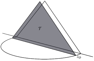
Figure 2: $\mathcal{E}$ and $\mathcal{T}$ surfaces over which the flux integrals (37) and (38) are computed.

Using equation (30), the integral on the surface $\mathcal{E}$ can be written out more explicitly:

$$-2\pi\int_{\mathcal{E}}d\Sigma^{a}\xi^{b}T^{B}_{ab}$$

$$=2\pi\int d\Omega_{d-2}\int_{z_{0}}^{R}\frac{dz}{z^{d-1}}\int_{0}^{\sqrt{R^{2}-z^{2}}}dr\,r^{d-2}\left[\frac{R^{2}-r^{2}-z^{2}}{2R}\right]\left[(\partial_{\tau}\phi)^{2}-\frac{\nabla^{2}_{E}\phi^{2}}{4z^{2}}\right].$$ (37)

This formula uses the solution on the Euclidean section in the bulk, with Euclidean time $\tau_{B}=it_{B}$. This is acceptable on the $t_{B}=0$ surface since the stress tensor there satisfies $T_{\tau\tau}^{B}=-T^{B}_{tt}$. The Laplacian $\nabla_{E}^{2}$ is hence the Euclidean AdS Laplacian. The $\mathcal{T}$ surface integral is

$$2\pi\int_{\mathcal{T}}d\Sigma^{a}\xi^{b}T^{B}_{ab}$$

$$=\frac{2\pi}{z_{0}^{d-1}}\int d\Omega_{d-2}\int_{0}^{R}dt\int_{0}^{R-t}dr\,r^{d-2}\left\{\left[\frac{R^{2}-r^{2}-t^{2}}{2R}\right]\partial_{z}\phi\partial_{t}\phi-\frac{z_{0}t}{R}\left[(\partial_{z}\phi)^{2}-\frac{\nabla^{2}\phi^{2}}{4z_{0}^{2}}\right]\right\}.$$ (38)

Here, note that the limits of integration have been set to coincide with $D^{+}(\Sigma)$, which is acceptable when taking $z_{0}\rightarrow 0$.

3 Producing excited states

This section describes the class of states that are formed from the Euclidean path integral prescription, and also discusses restrictions on the source function $f(x)$. One requirement is that the density matrix be Hermitian. For a density matrix constructed from a path integral as in (16), this translates to the condition that the deformed action $I_{0}+\int f\mathcal{O}$ be reflection symmetric about the $\tau=0$ surface on which the state is evaluated. When this is satisfied, $\rho$ defines a pure state [88]. Since this imposes $f(\tau,\vec{x})=f(-\tau,\vec{x})$, it gives the useful condition

$$\partial_{\tau}f(0,\vec{x})=0,$$ (39)

which simplifies the evaluation of the bulk integral (37).

Another condition on the state is that the stress tensor $T^{g}_{ab}$ of the deformed theory and the operator $\mathcal{O}$ have non-divergent expectation values, compared to the vacuum. These divergences are not independent, but are related to each other through Ward identities. The $\langle\mathcal{O}\rangle$ divergence is straightforward to evaluate,

$$\langle\mathcal{O}(0)\rangle =\frac{1}{N}\int\mathcal{D}\phi e^{-I_{0}}\left(1-\int f\mathcal{O}+\ldots\right)\mathcal{O}(0)$$ (40)

$$=-\int_{C(\delta)}d^{d}xf(x)\Big{\langle}\mathcal{O}(0)\mathcal{O}(x)\Big{\rangle}_{0},$$ (41)

where the $0$ subscript indicates a CFT vacuum correlation function. $C(\delta)$ refers to the regularization of this correlation function, which is a point-splitting cutoff for $|\tau|<\delta$. Note that $\delta$ is the same regulator appearing in the definition of the bulk scalar field, equation (31).

Only the change $\delta\langle\mathcal{O}\rangle$ in this correlation function relative to the deformed theory vacuum must be free of divergences. From the decomposition $f(x)=g(x)+\lambda(x)$, with $g(x)$ representing the deformation of the theory and $\lambda(x)$ the state deformation, one finds that the divergence in $\delta\langle\mathcal{O}\rangle$ comes from the coincident limit $x\rightarrow 0$. It can be extracted by expanding $\lambda(x)$ around $x=0$. The leading divergence is then

$$\delta\langle\mathcal{O}(0)\rangle_{\text{div}} =-\lambda(0)\int_{C(\delta)}d\tau\int d\Omega_{d-2}\int_{0}^{\infty}dr\frac{r^{d-2}c_{\Delta}}{(\tau^{2}+r^{2})^{\Delta}}$$

$$=-\lambda(0)\frac{2\Gamma(\Delta-\frac{d}{2}+\frac{1}{2})}{\sqrt{\pi}\,\Gamma(\Delta-\frac{d}{2})}\delta^{d-2\Delta}$$ (42)

When $\Delta\geq\frac{d}{2}$, a divergence in $\delta\langle\mathcal{O}\rangle$ exists unless $\lambda(0)=0$. Further, this must hold at every point on the $\tau=0$ surface, which leads to the requirement that $\lambda(0,\vec{x})=0$. Additionally, there can be subleading divergences proportional to $\delta^{d-2\Delta+2n}\partial_{\tau}^{2n}\lambda(0,\vec{x})$ for all integers $n$ where the $\delta$ exponent is negative or zero. Thus, the requirement on $\lambda$ is that its first $2q$ $\tau$-derivatives should vanish at $\tau=0$, where

$$q=\left\lfloor\Delta-\frac{d}{2}\right\rfloor.$$ (43)

We can also check that this condition leads to a finite value expectation value for the stress tensor, which for the deformed theory is

$$T^{g}_{ab}=\frac{2}{\sqrt{g}}\frac{\delta I}{\delta g^{ab}}=T^{0}_{ab}-g\mathcal{O}g_{ab},$$ (44)

where $T^{0}_{ab}$ is the stress tensor for the CFT. For the $T^{0}_{\tau\tau}$ component, the expectation value is

$$\langle T^{0}_{\tau\tau}(0)\rangle =\frac{1}{2}\iint_{C(\delta)}d^{d}x\,d^{d}yf(x)f(y)\Big{\langle}T^{0}_{\tau\tau}(0)\mathcal{O}(x)\mathcal{O}(y)\Big{\rangle}_{0}.$$ (45)

The divergence in this correlation function comes from $x,y\rightarrow 0$ simultaneously. It can be evaluated by expanding $f$ around $0$, and then employing Ward identities to relate it to the $\mathcal{O}\mathcal{O}$ two-point function (see, e.g.  section 2 of this chapter or Appendix D of [139]). The first order in $\lambda$ piece, which gives $\delta\langle T^{0}_{\tau\tau}\rangle$, is

$$\delta\langle T^{0}_{\tau\tau}\rangle_{\text{div}}=-g\lambda(0)2^{d-2\Delta}\frac{2\Gamma(\Delta-\frac{d}{2}+\frac{1}{2})}{\sqrt{\pi}\,\Gamma(\Delta-\frac{d}{2})}\delta^{d-2\Delta}.$$ (46)

The divergence in the actual energy density also receives a contribution from the $\mathcal{O}$ divergence (42). Using (44), this is found to be

$$\delta\langle T^{g}_{\tau\tau}\rangle_{\text{div}}=-g\lambda(0)\frac{2\Gamma(\Delta-\frac{d}{2}+\frac{1}{2})}{\sqrt{\pi}\,\Gamma(\Delta-\frac{d}{2})}(2^{d-2\Delta}-1)\delta^{d-2\Delta}.$$ (47)

As with the $\delta\langle\mathcal{O}\rangle$ divergence, requiring that $\lambda(0,\vec{x})=0$ ensures that the excited state has finite energy density. Subleading divergences and other components of $T^{g}_{ab}$ can be evaluated in a similar way, and lead to the same requirements on $\lambda$ as were found for the $\mathcal{O}$ divergences.

4 Entanglement entropy calculation

Now we compute the change in entanglement entropy for the state formed by the path integral with the deformed action $I=I_{0}+\int f\mathcal{O}$, with $f(x)=g(x)+\lambda(x)$ being a sum of the theory deformation $g$ and the state deformation $\lambda$. The bulk term $\delta S^{(2)}$ in plays an important role in this case. To evaluate this term, we need the solution for the scalar field in the bulk subject to the boundary conditions described in section 2. Since $\phi$ satisfies a linear field equation, so we may solve separately for the solution corresponding to $g$ and the solution corresponding to $\lambda$. The function $g(x)$ is taken to be spatially constant, and either constant in Euclidean time or set to zero at some IR length scale $L$. Its solution is most readily found by directly evaluating the integral (31), and we will discuss it separately in each of the cases $\Delta>\frac{d}{2}$, $\Delta<\frac{d}{2}$ and $\Delta=\frac{d}{2}$ considered below.

The solution for $\lambda(x)$ takes the same form in all three cases, so we begin by describing it. On the Euclidean section in Poincaré coordinates, the field equation (28) is

$$\left[z^{d+1}\partial_{z}(z^{-d+1}\partial_{z})+z^{2}\left(\partial_{\tau}^{2}+r^{-d+2}\partial_{r}(r^{d-2}\partial_{r})+r^{-2}\nabla^{2}_{\Omega_{d-2}}\right)\right]\phi-\Delta(\Delta-d)\phi=0,$$ (48)

where $\nabla^{2}_{\Omega_{d-2}}$ denotes the Laplacian on the $(d-2)$-sphere. Although one may consider arbitrary spatial dependence for the function $\lambda(x)$, the present calculation is concerned with the small ball limit, where the state may be taken uniform across the ball. We therefore restrict to $\lambda=\lambda(\tau)$. One can straightforwardly generalize to include corrections due to spatial dependence in $\lambda$, and these will produce terms suppressed in powers of $R^{2}$.

Equation (48) may be solved by separation of variables. The $\tau$ dependence is given by $\cos(\omega\tau)$, since it must be $\tau$-reflection symmetric. This leads to the equation for the $z$-dependence,

$$\partial_{z}^{2}\phi-\frac{d-1}{z}\partial_{z}\phi-\left(\omega^{2}+\frac{\Delta(\Delta-d)}{z^{2}}\right)\phi=0.$$ (49)

This has modified Bessel functions as solutions, and regularity as $z\rightarrow\infty$ selects the solution proportional to $z^{\frac{d}{2}}K_{\alpha}(\omega z)$, with

$$\alpha=\frac{d}{2}-\Delta.$$ (50)

Hence, the final bulk solution is

$$\phi_{\omega}=\lambda_{\omega}\left(\frac{\omega}{2}\right)^{\Delta-\frac{d}{2}}\frac{2z^{\frac{d}{2}}K_{\alpha}(\omega z)}{\Gamma(\Delta-\frac{d}{2})}\,\cos\omega\tau.$$ (51)

where the normalization has been chosen so that the coefficient of $z^{d-\Delta}$ in the near-boundary expansion is

$$\lambda=\lambda_{\omega}\cos(\omega\tau).$$ (52)

A single frequency solution will not satisfy the requirement derived in section 3 that $\lambda(0,\vec{x})$ and its first $2q$ $\tau$-derivatives vanish (where $q$ was given in (43)). Instead, $\lambda$ must be constructed from a wavepacket of several frequencies,

$$\lambda(\tau)=\int_{0}^{\infty}d\omega\lambda_{\omega}\cos(\omega\tau),$$ (53)

with Fourier components $\lambda_{\omega}$ satisfying

$$\int_{0}^{\infty}d\omega\,\omega^{2n}\lambda_{\omega}=0$$ (54)

for all nonnegative integers $n\leq q$. Finally, the coefficients $\lambda_{\omega}$ should fall off rapidly before $\omega$ becomes larger than $R^{-1}$, since such a state would be considered highly excited relative to the scale set by the ball size.

Using these solutions, we may proceed with the entanglement entropy calculation. The answer for $\Delta>\frac{d}{2}$ in section 1 comes from a simple application of the formula derived in [139]. In section 2 when considering $\Delta<\frac{d}{2}$, we must introduce a new element into the calculation to deal with IR divergences that arise. This is just a simple IR cutoff in the theory deformation $g(x)$, which allows a finite answer to emerge, although a new set of divergences along the timelike surface $\mathcal{T}$ must be shown to cancel. A similar story emerges in section 3 for $\Delta=\frac{d}{2}$, although extra care must be taken due to the presence of logarithms in the solutions.

1 $\Delta>\frac{d}{2}$

The full bulk scalar field separates into two parts,

$$\phi=\phi_{0}+\phi_{\omega},$$ (55)

with $\phi_{\omega}$ from (51) describing the state deformation, while $\phi_{0}$ corresponds to the theory deformation $g(x)$. Since no IR divergences arise at this order in perturbation theory when $\Delta>\frac{d}{2}$, we can take $g$ to be constant everywhere. The solution in the bulk on the Euclidean section then takes the simple form

$$\phi_{0}=gz^{d-\Delta}.$$ (56)

Given these two solutions, the bulk contribution to $\delta S^{(2)}$ may be computed using equation (37). Note that $\partial_{\tau}\phi=0$ on the $\tau=0$ surface, so we only need the $\nabla^{2}\phi^{2}$ term in the integrand. Before evaluating this term, it is useful to expand $\phi_{\omega}$ near $z=0$. This expansion takes the form

$$\phi_{\omega}=\left[\lambda_{\omega}z^{d-\Delta}\sum_{n=0}^{\infty}a_{n}(\omega z)^{2n}+\beta_{\omega}z^{\Delta}\sum_{n=0}^{\infty}b_{n}(\omega z)^{2n}\right]\cos(\omega\tau),$$ (57)

where

$$\beta_{\omega}=\lambda_{\omega}\left(\frac{\omega}{2}\right)^{2\Delta-d}\frac{\Gamma(\frac{d}{2}-\Delta)}{\Gamma(\Delta-\frac{d}{2})},$$ (58)

and the coefficients $a_{n}$ and $b_{n}$ are given in appendix 1.A. The $O(\lambda^{1})$ term in $\phi^{2}$ is $2\phi_{0}\phi_{\omega}$, and this modifies the power series (57) by changing the leading powers to $z^{2(d-\Delta)}$ and $z^{d}$. The Laplacian in the bulk is

$$\nabla^{2}=z^{2}\partial_{\tau}^{2}+z^{d+1}\partial_{z}(z^{-d+1}\partial_{z}).$$ (59)

Acting on the $\phi_{0}\phi_{\omega}$ series, the effect of the $\tau$ derivative is to multiply by $-\omega^{2}z^{2}$, which shifts each term to one higher term in the series. The $z$ derivatives do no change the power of $z$, but rather multiply each term by a constant, $2(d-\Delta+n)(d-2\Delta+2n)$ for the $a_{n}$ series and $2n(d+2n)$ for the $b_{n}$ series (note in particular it annihilates the first term in the $b_{n}$ series). After this is done, the series may be reorganized for $\tau=0$ as

$$2\nabla^{2}\phi_{0}\phi_{\omega}=2g\lambda_{\omega}z^{2(d-\Delta)}\sum_{n=0}^{\infty}c_{n}(\omega z)^{2n}+2g\beta_{\omega}z^{d}\sum_{n=1}^{\infty}d_{n}(\omega z)^{2n},$$ (60)

with the coefficients $c_{n}$ and $d_{n}$ computed in appendix 1.A.

From this, we simply need to evaluate the integral (37) for each term in the series. For a given term of the form $Az^{\eta}$, the contribution to $\delta S^{(2)}$ is

$$\delta S^{(2)}_{\eta} =-\frac{\pi}{2}\Omega_{d-2}\int_{z_{0}}^{R}\frac{dz}{z^{d+1}}\int_{0}^{\sqrt{R^{2}-z^{2}}}dr\,r^{d-2}\left[\frac{R^{2}-r^{2}-z^{2}}{2R}\right]Az^{\eta}$$ (61)

$$=-A\frac{\pi\Omega_{d-2}}{4(d^{2}-1)}\left[R^{\eta}\,\frac{\Gamma(\frac{d}{2}+\frac{3}{2})\Gamma(\frac{\eta}{2}-\frac{d}{2})}{\Gamma(\frac{\eta}{2}+\frac{3}{2})}+\frac{R^{d}z_{0}^{\eta-d}\tensor[_{2}]{F}{{}_{1}}\left(-\frac{d+1}{2},\frac{\eta-d}{2};\frac{\eta-d}{2}+1;\frac{z_{0}^{2}}{R^{2}}\right)}{\frac{\eta}{2}-\frac{d}{2}}\right].$$ (62)

The second term in this expression contains a set of divergences at $z_{0}\rightarrow 0$ for all values of $\eta<d$. These arise exclusively from the $c_{n}$ series in (60). In general, the expansion of the hypergeometric function near $z_{0}=0$ can produce subleading divergences, which mix between different terms from the series (60). These divergences eventually must cancel against compensating divergences that arise from the $\mathcal{T}$ surface integral in (38). Although we do not undertake a systematic study of these divergences, we may assume that they cancel out because the cutoff surface at $z_{0}$ was chosen arbitrarily, and the original integral (27) made no reference to it. Thus, we may simply discard these $z_{0}$ dependent divergences, and are left with only the first term in (62).

There is another reason for discarding the $z_{0}$ divergences immediately: they only arise in states with divergent energy density. The coefficient of a term with a $z_{0}$ divergence is $2gc_{n}\omega^{2n}\lambda_{\omega}$. The final answer for the entanglement entropy will involve integrating over all values of $\omega$. But the requirement of finite energy density (54) shows that all terms with $n\leq q$, corresponding to $\eta\leq 2d-2\Delta+2q$, will vanish from the final result. Given the definition of $q$ in (43), these are precisely the terms in (62) that have divergences in $z_{0}$. Note that since $\beta_{\omega}\propto\omega^{2\Delta-d}$, which is generically a non-integer power, the integral over $\omega$ will not vanish, so all the $\beta_{\omega}$ terms survive.

The resulting bulk contribution to the entanglement entropy at order $\lambda g$ is

$$\delta S^{(2)}_{\mathcal{E},\lambda g}=-\frac{g\pi^{\frac{d}{2}+\frac{1}{2}}}{4}\int_{0}^{\infty}d\omega\left[\lambda_{\omega}R^{2(d-\Delta)}\sum_{n=q+1}^{\infty}\right. c_{n}\frac{\Gamma(\frac{d}{2}-\Delta+n)}{\Gamma(d-\Delta+\frac{3}{2}+n)}(\omega R)^{2n}$$

$$+\;\beta_{\omega}R^{d}\sum_{\hphantom{+}n=1\hphantom{+}}^{\infty} \left.\vphantom{\sum_{n=1}^{\infty}}d_{n}\frac{\Gamma(\frac{d}{2}+n)}{\Gamma(\frac{d}{2}+\frac{3}{2}+n)}(\omega R)^{2n}\right].$$ (63)

This expression shows that the lowest order pieces scale as $R^{2(d-\Delta+q+1)}$ and $R^{d+2}$, which both become subleading with respect to the $R^{d}$ scaling of the $\delta S^{(1)}$ piece for small ball size. Note that a similar technique could extend this result to spatially dependent $\lambda(x)$, and simply would amount to an additional series expansion.

One could perform a similar analysis for the $O(\lambda^{2})$ contribution from $\delta S^{(2)}$. The series of $\nabla^{2}\phi_{\omega}\phi_{\omega^{\prime}}$ would organize into three series, with leading coefficients $\lambda_{\omega}\lambda_{\omega^{\prime}}z^{2(d-\Delta)}$, $(\beta_{\omega}\lambda_{\omega^{\prime}}+\lambda_{\omega}\beta_{\omega^{\prime}})z^{d}$, and $\beta_{\omega}\beta_{\omega^{\prime}}z^{2\Delta}$. After integrating over $\omega$ and $\omega^{\prime}$, and noting which terms vanish due to the requirement (54), one would find the leading contribution going as $\beta^{2}R^{2\Delta}$. The precise value of this term is

$$\delta S^{(2)}_{\lambda^{2}}=-\frac{\pi\Omega_{d-2}}{d^{2}-1}R^{2\Delta}\big{(}\delta\langle\mathcal{O}\rangle\big{)}^{2}\,\frac{\Delta\Gamma(\frac{d}{2}+\frac{3}{2})\Gamma(\Delta-\frac{d}{2}+1)}{(2\Delta-d)^{2}\Gamma(\Delta+\frac{3}{2})},$$ (64)

which is quite similar to the $R^{2\Delta}$ term in equation (1). This is again subleading when $\Delta>\frac{d}{2}$, but the same terms show up for $\Delta\leq\frac{d}{2}$ in sections 2 and 3, where they become the dominant contribution when $R$ is taken small enough. The importance of these second order terms in the small $R$ limit was first noted in [141].

The remaining pieces to calculate come from the integral over $\mathcal{T}$ given by (38), and $\delta S^{(1)}$ in (23), which just depends on $\delta\langle T^{0}_{00}\rangle$. When $\Delta>\frac{d}{2}$, the only contribution from the $\mathcal{T}$ surface integral is near $t_{B}\sim z\rightarrow 0$. These terms were analyzed in appendix E of [139], and were found to give two types of contributions. The first were counter terms that cancel against the divergences in the bulk as well as the divergence in $\delta S^{(1)}$. Although subleading divergences were not analyzed, these can be expected to cancel in a predictable way. We also already argued that such terms are not relevant for the present analysis, due to the requirement of finite energy density. The second type of term is finite, and takes the form

$$\delta S^{(2)}_{\mathcal{T},\text{finite}}=-2\pi\Delta\int_{\Sigma}\zeta^{t}g\beta.$$ (65)

The relation between $\beta$ and $\delta\langle\mathcal{O}\rangle$ identified in (34) implies from equation (58),

$$\delta\langle\mathcal{O}\rangle=\lambda_{\omega}\frac{2\Gamma(\frac{d}{2}-\Delta+1)}{\Gamma(\Delta-\frac{d}{2})}\left(\frac{\omega}{2}\right)^{2\Delta-d},$$ (66)

and assuming the ball is small enough so that this expectation value may be considered constant, (65) evaluates to

$$\delta S^{(2)}_{\mathcal{T},\text{finite}}=2\pi\frac{\Omega_{d-2}R^{d}}{d^{2}-1}\left[\frac{\Delta}{2\Delta-d}g\delta\langle\mathcal{O}\rangle\right].$$ (67)

Similarly, taking $\delta\langle T^{0}_{00}\rangle$ to be constant over the ball, the final contribution is the variation of the modular Hamiltonian piece, given by

$$\delta S^{(1)}=2\pi\int_{\Sigma}\zeta^{t}\delta\langle T^{0}_{00}\rangle=2\pi\frac{\Omega_{d-2}R^{d}}{d^{2}-1}\delta\langle T^{0}_{00}\rangle.$$ (68)

Before writing the final answer, it is useful to write $\delta\langle\mathcal{O}\rangle$ in terms of the trace of the stress tensor of the deformed theory, $T^{g}$. The two are related by the dilatation Ward identity, which gives [148]

$$\delta\langle T^{g}\rangle=(\Delta-d)g\delta\langle\mathcal{O}\rangle.$$ (69)

Then, using the definition of the deformed theory’s stress tensor (44) and summing up the contributions (63), (67), and (68), the total variation of the entanglement entropy at $O(\lambda^{1}g^{1})$ is

$$\delta S_{\lambda g}=2\pi\frac{\Omega_{d-2}R^{d}}{d^{2}-1}\left[\delta\langle T^{g}_{00}\rangle-\frac{1}{2\Delta-d}\delta\langle T^{g}\rangle\right]+\delta S^{(2)}_{\mathcal{E},\lambda g}.$$ (70)

Since $\delta S^{(2)}_{\mathcal{E},\lambda g}$ is subleading, this matches the result (1) quoted in the introduction, apart from the $R^{2\Delta}$ term, which is not present because we have arranged for the renormalized vev $\langle\mathcal{O}\rangle_{g}$ to vanish. However, as noted in equation (64), we do find such a term at second order in $\lambda$.

2 $\Delta<\frac{d}{2}$

Extending the above calculation to $\Delta<\frac{d}{2}$ requires the introduction of one novel element: a modification of the coupling $g(x)$ to include an IR cutoff. It is straightforward to see why this regulator is needed. The perturbative calculation of the entanglement entropy involves integrals of the two point correlator over all of space, schematically of the form

$$\int d^{d}xg(x)\Big{\langle}\mathcal{O}(0)\mathcal{O}(x)\Big{\rangle}_{0}=\int d^{d}x\frac{c_{\Delta}g(x)}{x^{2\Delta}}.$$ (71)

If this is cut off at a large distance $L$, the integral scales as $L^{d-2\Delta}$ (or $\log L$ for $\Delta=\frac{d}{2}$) when the coupling $g(x)$ is constant. This clearly diverges for $\Delta\leq\frac{d}{2}$.

The usual story with IR divergences is that resumming the higher order terms remedies the divergence, effectively imposing an IR cut off. Presumably this cut off is set by the scale of the coupling $L_{\text{eff}}\sim g^{\frac{1}{\Delta-d}}$, but since it arises from higher order correlation functions, it may also depend on the details of the underlying CFT. Although it may still be possible to compute these IR effects in perturbation theory [149, 150, 151], this goes beyond the techniques employed in the present work. However, if we work on length scales small compared to the IR scale, it is possible to capture the qualitative behavior by simply putting in an IR cut off by hand (see [152] for a related approach). We implement this IR cutoff by setting the coupling $g(x)$ to zero when $|\tau|\geq L$. We may then express the final answer in terms of the vev $\langle\mathcal{O}\rangle_{g}$, which implicitly depends on the IR regulator $L$.

The bulk term $\delta S^{(2)}$ involves a new set of divergences from the $\mathcal{T}$ surface integral that were not present in the original calculation for $\Delta>\frac{d}{2}$ [139]. To compute these divergences and show that they cancel, we will need the real time behavior of the bulk scalar fields, in addition to its behavior at $t=0$. These are described in appendix 1. The important features are that $\phi_{0}$ on the $t=0$ surface takes the form

$$\phi_{0}=-\frac{\langle\mathcal{O}\rangle_{g}}{2\Delta-d}z^{\Delta}+gz^{d-\Delta},$$ (72)

and the vev $\langle\mathcal{O}\rangle_{g}$ is determined in terms of the IR cutoff $L$ by

$$\langle\mathcal{O}\rangle_{g}=2gL^{d-2\Delta}\frac{\Gamma(\Delta-\frac{d}{2}+\frac{1}{2})}{\sqrt{\pi}\,\Gamma(\Delta-\frac{d}{2})}.$$ (73)

For $t>0$, the time-dependent solution is given by

$$\phi_{0}=-\frac{\langle\mathcal{O}\rangle_{g}}{2\Delta-d}z^{\Delta}+gz^{d-\Delta}F(t/z),$$ (74)

where the function $F$ is defined in equation (116). To compute the divergences along $\mathcal{T}$, the form of this function is needed in the region $t\gg z$, where it simply becomes

$$F(t/z)\xrightarrow{t\gg z}B\left(\frac{t}{z}\right)^{d-2\Delta},$$ (75)

with the proportionality constant $B$ given in equation (117). The field $\phi_{\omega}$ behaves similarly as long as $\omega^{-1}\gg z,t$. In particular, it has the same form as $\phi_{0}$ in equations (72) and (74), but with $g$ replaced by $\lambda_{\omega}$, and $\langle\mathcal{O}\rangle_{g}$ replaced with $\delta\langle\mathcal{O}\rangle$, given by

$$\delta\langle\mathcal{O}\rangle=\lambda_{\omega}\frac{2\Gamma(\frac{d}{2}-\Delta+1)}{\Gamma(\Delta-\frac{d}{2})}\left(\frac{\omega}{2}\right)^{2\Delta-d},$$ (76)

which is the same relation as for $\Delta>\frac{d}{2}$, equation (66).

Armed with these solutions, we can proceed to calculate $\delta S^{(2)}$. In this calculation, the contribution from the timelike surface $\mathcal{T}$ now has a novel role. Before, when $\Delta>\frac{d}{2}$, the integral from this surface died off as $z\rightarrow 0$ in the region $t_{B}>z$, and hence the integral there did not need to be evaluated. For $\Delta<\frac{d}{2}$, rather than dying off, this integral is now leads to divergences as $z\rightarrow 0$. These divergences either cancel among themselves, or cancel against divergences coming from bulk Euclidean surface $\mathcal{E}$, so that a finite answer is obtained in the end. These new counterterm divergences seem to be related to the alternate quantization in holography [146, 141], which invokes a different set of boundary counterterms when defining the bulk AdS action. It would be interesting to explore this relation further.

At first order in $g$ and $\lambda$, three types of terms will appear, proportional to each of $\langle\mathcal{O}\rangle_{g}\,\delta\langle\mathcal{O}\rangle$, $(g\delta\langle\mathcal{O}\rangle+\lambda(0)\langle\mathcal{O}\rangle_{g})$, or $g\lambda(0)$. Here, we allow $\lambda(0)\neq 0$ because there are no UV divergences arising in the energy density or $\mathcal{O}$ expectation values when $\Delta<\frac{d}{2}$. The descriptions of the contribution from each of these terms are given below, and the details of the surface integrals over $\mathcal{E}$ and $\mathcal{T}$ are contained in appendix 1.

The $\langle\mathcal{O}\rangle_{g}\delta\langle\mathcal{O}\rangle$ term has both a finite and a divergent piece coming from the integral over $\mathcal{E}$ (see equation (132)). This divergence is canceled by the $\mathcal{T}$ integral in the region $t_{B}\gg z_{0}$. This is interesting since it differs from the $\Delta>\frac{d}{2}$ case, where the bulk divergence was canceled by the $\mathcal{T}$ integral in the region $t_{B}\lesssim z_{0}$. The final finite contribution from this term is

$$\delta S^{(2)}_{\mathcal{E},1}=-2\pi\langle\mathcal{O}\rangle_{g}\,\delta\langle\mathcal{O}\rangle\frac{\Omega_{d-2}}{d^{2}-1}R^{2\Delta}\frac{\Delta\Gamma(\frac{d}{2}+\frac{3}{2})\Gamma(\Delta-\frac{d}{2}+1)}{(2\Delta-d)^{2}\Gamma(\Delta+\frac{3}{2})}.$$ (77)

It is worth noting that we can perform the exact same calculation with $\langle\mathcal{O}\rangle_{g}\delta\langle\mathcal{O}\rangle$ replaced by $\frac{1}{2}\delta\langle\mathcal{O}\rangle^{2}$ to compute the second order in $\lambda$ change in entanglement entropy. The value found in this case agrees with holographic results [141].

The $g\delta\langle\mathcal{O}\rangle+\lambda(0)\langle\mathcal{O}\rangle_{g}$ term receives no contribution from the $\mathcal{E}$ surface at leading order since this term in $\phi^{2}$ scales as $z^{d}$ in the bulk, and the $z$-derivatives in the Laplacian $\nabla^{2}$ annihilate such a term. The surface $\mathcal{T}$ produces a finite term, plus a collection of divergent terms from both regions $t\sim z$ and $t\gg z$, which cancel among themselves. The finite term is given by

$$\delta S^{(2)}_{\mathcal{T},2}=2\pi\frac{\Omega_{d-2}R^{d}\Delta}{(d^{2}-1)(2\Delta-d)}(g\delta\langle\mathcal{O}\rangle+\lambda(0)\langle\mathcal{O}\rangle_{g}),$$ (78)

which is exactly analogous to the term (67) found for the case $\Delta>\frac{d}{2}$.

Finally, the term with coefficient $\lambda(0)g$ produces subleading terms, scaling as $R^{2(d-\Delta+n)}$ for positive integers $n$. Since these terms are subleading, we do not focus on them further. In this case, it must also be shown that the divergences appearing in the $\mathcal{T}$ cancel amongst themselves, since no divergences arise from the $\mathcal{E}$ integral. The calculations in appendix 1 verify that this indeed occurs.

We are now able to write down the final answer for the change in entanglement entropy for $\Delta<\frac{d}{2}$. The contribution from $\delta S^{(1)}$ is exactly the same as the $\Delta>\frac{d}{2}$ case, and is given by (68). Following the same steps that led to equation (70), the contributions from the finite piece of $\delta S^{(2)}_{\mathcal{E},1}$ in (132) and $\delta S^{(2)}_{\mathcal{T},2}$ in (138) combine with $\delta S^{(1)}$ to give

$$\delta S_{\lambda g}=\frac{2\pi\Omega_{d-2}}{d^{2}-1}\left[R^{d}\left(\langle T^{g}_{00}\rangle-\frac{1}{2\Delta-d}\langle T^{g}\rangle\right)-R^{2\Delta}\langle\mathcal{O}\rangle_{g}\delta\langle\mathcal{O}\rangle\frac{\Delta\Gamma(\frac{d}{2}+\frac{3}{2})\Gamma(\Delta-\frac{d}{2}+1)}{(2\Delta-d)^{2}\Gamma(\Delta+\frac{3}{2})}\right],$$ (79)

where we have set $\lambda(0)=0$ for simplicity and to match the expression for $\Delta>\frac{d}{2}$, which required $\lambda(0)=0$.

3 $\Delta=\frac{d}{2}$

Similar to the $\Delta<\frac{d}{2}$ case, there are IR divergences that arise when $\Delta=\frac{d}{2}$. These are handled as before with an IR cutoff $L$, on which the final answer explicitly depends. A new feature arises, however, when expressing the answer in terms of $\langle\mathcal{O}\rangle_{g}$ rather than $L$: the appearance of a renormalization scale $\mu$. The need for this renormalization scale can be seen by examining the expression for $\langle\mathcal{O}\rangle_{g}$, which depends on the $\mathcal{O}\mathcal{O}$ two-point function with $\Delta=\frac{d}{2}$:

$$\langle\mathcal{O}\rangle_{g}=-\int d^{d}x\frac{gc^{\prime}_{\Delta}}{x^{d}}=-gc^{\prime}_{\Delta}\frac{\pi^{\frac{d}{2}}}{\Gamma(\frac{d}{2})}\int\frac{d\tau}{\tau}.$$ (80)

This has a logarithmic divergence near $x=0$ which must be regulated. The UV-divergent piece can be extracted using the point-splitting cutoff for $|\tau|<\delta$; however, there is an ambiguity in identifying this divergence since the upper bound of this integral cannot be sent to $\infty$. The appearance of the renormalization scale is related to matter conformal anomalies that exist for special values of $\Delta$ [153, 148, 154]. Thus we must impose an upper cutoff on the integral, which introduces the renormalization scale $\mu^{-1}$. The divergent piece of $\langle\mathcal{O}\rangle_{g}$ is then

$$\langle\mathcal{O}\rangle_{g}^{\text{div.}}=gc^{\prime}_{\Delta}\frac{\pi^{\frac{d}{2}}}{\Gamma(\frac{d}{2})}2\log\mu\delta.$$ (81)

Now we can determine the renomalized vev of $\mathcal{O}$, using the IR-regulated $\tau$ integral,

$$\langle\mathcal{O}\rangle_{g}^{\text{ren.}}=\langle\mathcal{O}\rangle_{g}-\langle\mathcal{O}\rangle_{g}^{\text{div.}} =-\int^{L}d\tau\int d^{d-1}x\frac{gc^{\prime}_{\Delta}}{x^{d}}-gc^{\prime}_{\Delta}\frac{\pi^{\frac{d}{2}}}{\Gamma(\frac{d}{2})}2\log\mu\delta$$ (82)

$$=-gc^{\prime}_{\Delta}\frac{\pi^{\frac{d}{2}}}{\Gamma(\frac{d}{2})}2\log\mu L.$$ (83)

The final answer we derive for the entanglement entropy when $\Delta=\frac{d}{2}$ will depend on $\log L$ but not on explicitly $\mu$ or $\langle\mathcal{O}\rangle_{g}$. Only after rewriting it in terms of $\langle\mathcal{O}\rangle^{\text{ren.}}_{g}$ does the $\mu$ dependence appear.

One other small modification is necessary when $\Delta=\frac{d}{2}$. The normalization $c_{\Delta}$ for the $\mathcal{O}\mathcal{O}$ two point function defined in (32) has a double zero at $\Delta=\frac{d}{2}$ which must be removed. This is easily remedied by dividing by $(2\Delta-d)^{2}$ [146, 155], so that the new constant appearing in the two point function is

$$c^{\prime}_{\Delta}=\frac{\Gamma(\Delta)}{2\pi^{\frac{d}{2}}\Gamma(\Delta-\frac{d}{2}+1)}\;\xrightarrow{\hphantom{n}\Delta\rightarrow\frac{d}{2}\hphantom{n}}\;\frac{\Gamma(\frac{d}{2})}{2\pi^{\frac{d}{2}}}.$$ (84)

This change affects the normalization of the bulk field $\phi$ by dividing by a single factor of $1/(2\Delta-d)$, so that

$$\phi(x_{B})=\frac{\Gamma(\frac{d}{2})}{2\pi^{\frac{d}{2}}}\int_{C(\delta)}d\tau\int d^{d-1}\vec{x}\frac{z^{\Delta}f(\tau,\vec{x})}{(z^{2}+(\tau-it_{B})^{2}+(\vec{x}-\vec{x}_{B})^{2})^{\Delta}}.$$ (85)

These are all the components needed to proceed with the calculation of the entanglement entropy. As before, we solve for the bulk field $\phi_{0}$ associated with a constant coupling $g$, set to zero for $|\tau|>L$. The $\phi_{\omega}$ field associated with the state deformation $\lambda=\lambda_{\omega}\cos\omega\tau$ is again given by a modified Bessel function on the Euclidean section. Its form along the timelike surface $\mathcal{T}$ is derived from the integral representation (85), and particular care must be taken in the region $t_{B}\sim z$, where a divergence in $\delta$ appears. Although this divergence is not present if we require $\lambda(0)=0$, we analyze the terms that it produces for generality. This $\delta$ divergence is shown to cancel against a similar divergence in $\delta S^{(1)}$ related to the divergence in the $\langle T_{00}\mathcal{O}\mathcal{O}\rangle$ three-point function.

The full real-time solutions for $\phi_{0}$ and $\phi_{\omega}$ are given in appendix 2. The $\phi_{0}$ solution from equation (124) takes the form

$$\phi_{0}=gz^{\frac{d}{2}}G(t_{B}/z,\delta/z,L/z),$$ (86)

with the function $G$ defined in equation (125). The dependence of this function on $\delta$ is needed only in the region $t_{B}\sim z$; everywhere else it can safely be taken to zero. On the $\mathcal{E}$ surface where $t_{B}=0$, the solution in the limit $L\gg z$ is

$$\phi_{0}=gz^{\frac{d}{2}}\log\frac{2L}{z}=-\langle\mathcal{O}\rangle_{g}^{\text{ren.}}-gz^{\frac{d}{2}}\log\frac{\mu z}{2},$$ (87)

where the second equality uses the value of $\langle\mathcal{O}\rangle_{g}^{\text{ren.}}$ derived in (83). We also need $\phi_{0}$ in the region $t_{B}\gg z$, given by

$$\phi_{0}=gz^{\frac{d}{2}}\log\frac{L}{t_{B}}.$$ (88)

For $\phi_{\omega}$, the solution on the $\mathcal{E}$ surface is still given by a modified Bessel function as in equation (51), but must be divided by $(2\Delta-d)$ according to our new normalization (85),

$$\phi_{\omega}=\lambda_{\omega}z^{\frac{d}{2}}K_{0}(\omega z)\xrightarrow{z\rightarrow 0}-\lambda_{\omega}z^{\frac{d}{2}}\left(\gamma_{E}+\log\frac{\omega z}{2}\right).$$ (89)

By writing the argument of the $\log$ term as in equation (87), one can read off the renormalized operator expectation value,

$$\delta\langle\mathcal{O}\rangle^{\text{ren.}}=\lambda_{\omega}\left(\gamma_{E}+\log\frac{\omega}{\mu}\right).$$ (90)

Beyond $t_{B}=0$, as long as $\omega^{-1}\gg t_{B}$, the solution can be written in a similar form as (86). When $t_{B}\gg z$, this is given by

$$\phi_{\omega}=-\lambda_{\omega}z^{\frac{d}{2}}(\gamma_{E}+\log\omega t_{B}).$$ (91)

Now that we have the form of the solutions on the surfaces $\mathcal{E}$ and $\mathcal{T}$, the entanglement calculation contains four parts. The first is the integral over $\mathcal{E}$, where a $\log z_{0}$ divergence appears. This cancels against a collection of divergences from the $\mathcal{T}$ surface. The second part is the $\mathcal{T}$ surface near $t_{B}\sim z$. This region produces more divergences in $z_{0}$ and $\delta$, some of which cancel the bulk divergence. The third part is the integral over $\mathcal{T}$ for $t_{B}\gg z$, which eliminates the remaining $z_{0}$ divergences. Finally, an additional divergence from the stress tensor in $\delta S^{(1)}$ cancels the $\delta$ divergence, producing a finite answer.

Appendix 2 describes the details of these calculations. In the end, the contributions from equations (146), (142), (152), (162) and (171) combine together to give the following total change in entanglement entropy, at $O(\lambda^{1}g^{1})$,

$$\delta S_{\lambda_{\omega}g} =2\pi\frac{\Omega_{d-2}R^{d}}{d^{2}-1}\left\{\delta\langle T^{0}_{00}\rangle^{\text{ren.}}+g\lambda_{\omega}\left[\frac{d}{2}\log\left(\frac{2L}{R}\right)\left(\gamma_{E}+\log\frac{\omega R}{2}\right)\right.\right.$$

$$\left.\left.+\frac{d}{4}H_{\frac{d+1}{2}}\left(\gamma_{E}+\log\frac{R^{2}\omega}{4L}\right)-\log\mu R-\frac{1}{8}\left(H^{(2)}_{\frac{d+1}{2}}+H_{\frac{d+1}{2}}(H_{\frac{d+1}{2}}-2)\right)\right]\right\}.$$ (92)

This is the answer for a single frequency $\omega$ in the state deformation function $\lambda(x)$. Since $\lambda(0)\neq 0$, this result cannot be immediately interpreted as the entanglement entropy of an excited state, since the state has a divergent expectation value for $\mathcal{O}$. To get the entanglement entropy for an excited state, we should integrate over all frequencies, and use the fact that $\int d\omega\lambda_{\omega}=0$. When this is done, all terms with no $\log\omega$ dependence drop out. Also, we no longer need to specify that operator expectation values are renormalized, since the change in expectation values between two states is finite and scheme-independent.

We would like to express the answer in terms of $\delta\langle\mathcal{O}\rangle$. By integrating equation (90) over all frequencies and using that $\lambda(0)=0$, we find

$$\delta\langle\mathcal{O}\rangle=\int_{0}^{\infty}d\omega\,\lambda_{\omega}\log\omega.$$ (93)

With this, the total change in entanglement entropy for nonsingular states coming from integrating 92 over all frequencies is

$$\delta S_{\lambda g}=2\pi\frac{\Omega_{d-2}R^{d}}{d^{2}-1}\left[\delta\langle T^{0}_{00}\rangle+g\frac{d}{2}\delta\langle\mathcal{O}\rangle\left(\frac{1}{2}H_{\frac{d+1}{2}}+\log\frac{2L}{R}\right)\right].$$ (94)

This can be expressed in terms of the deformed theory’s stress tensor $T^{g}_{00}$ and trace $T^{g}$ using equations (44) and (69),

$$\delta S_{\lambda g}=2\pi\frac{\Omega_{d-2}R^{d}}{d^{2}-1}\left[\delta\langle T^{g}_{00}\rangle+\delta\langle T^{g}\rangle\left(\frac{2}{d}-\frac{1}{2}H_{\frac{d+1}{2}}+\log\frac{R}{2L}\right)\right].$$ (95)

Although the answer is scheme-independent in the sense that $\mu$ does not explicitly appear, there is a dependence on the IR cutoff $L$. This cutoff is related to the renormalized vev $\langle\mathcal{O}\rangle^{\text{ren.}}_{g}$ via (83), which does depend on the renormalization scheme. Thus the dependence on $L$ in the above answer can be traded for $\langle\mathcal{O}\rangle_{g}^{\text{ren.}}$, at the cost of introducing (spurious) $\mu$-dependence,

$$\delta S_{\lambda g}=2\pi\frac{\Omega_{d-2}R^{d}}{d^{2}-1}\left[\delta\langle T^{g}_{00}\rangle+\delta\langle T^{g}\rangle\left(\frac{2}{d}-\frac{1}{2}H_{\frac{d+1}{2}}+\log\frac{\mu R}{2}\right)-\frac{d}{2}\langle\mathcal{O}\rangle_{g}\delta\langle\mathcal{O}\rangle\right],$$ (96)

which is the result quoted in the introduction, equation (2).

5 Discussion

The equivalence between the Einstein equation and maximum vacuum entanglement of small balls relies on a conjecture about the behavior of the entanglement entropy of excited states, equation (11). This chapter has sought to check the conjecture in CFTs deformed by a relevant operator. In doing so, we have derived new results on the behavior of excited state entanglement entropy in such theories, encapsulated by equations (1) and (2). These results agree with holographic calculations [141] that employ the Ryu-Takayanagi formula. Thus, this chapter extends those results to any CFT, including those which are not thought to have holographic duals.

For deforming operators of dimension $\Delta>\frac{d}{2}$ considered in section 1, the calculation is a straightforward application of Faulkner’s method for computing entanglement entropies [139]. One subtlety in this case is the presence of UV divergences in $\delta\langle\mathcal{O}\rangle$ and $\delta\langle T^{0}_{00}\rangle$ unless the state deformation function $\lambda(x)$ is chosen appropriately. As discussed in section 3, this translates to the condition that $\lambda$ and sufficiently many of its $\tau$-derivatives vanish on the $\tau=0$ surface. When the entanglement entropy of the state is calculated, this condition implies that terms scaling with the ball radius as $R^{2(d-\Delta+n)}$, which are present for generic $\lambda(x)$, vanish, where $n$ is a positive integer less than or equal to $\left\lfloor\Delta-\frac{d}{2}\right\rfloor$. As $R$ approaches zero, these terms dominate over the energy density term, which scales as $R^{d}$. This shows that regularity of the state translates to the dominance of the modular Hamiltonian term in the small ball limit when $\Delta>\frac{d}{2}$. The subleading terms arising from this calculation are given in equation (63).

Section 2 then extends this result to operators of dimension $\Delta<\frac{d}{2}$. In this case, IR divergences present a novel facet to the calculation. To deal with these divergences, we impose an IR cutoff on the coupling $g(x)$ at scale $L$. A more complete treatment of the IR divergences would presumably involve resumming higher order contributions, which then would effectively impose an IR cutoff in the lower order terms. This cutoff should be of the order $L_{\text{eff.}}\sim g^{\frac{1}{\Delta-d}}$, but can depend on other details of the CFT, including any large parameters that might be present. Note this nonanalytic dependence of the IR cutoff on the coupling signals nonperturbative effects are at play [156, 157]. After the IR cutoff is imposed, the calculation of the entanglement entropy proceeds as before. In the final answer, equation (1), the explicit dependence on the IR cutoff is traded for the renormalized vacuum expectation value $\langle\mathcal{O}\rangle_{g}$. This expression agrees with the holographic calculation to first order in $\delta\langle\mathcal{O}\rangle$ in the case that $\langle\mathcal{O}\rangle_{g}$ is nonzero [141].

Finally, the special case of $\Delta=\frac{d}{2}$ is addressed in section 3. Here, both UV and IR divergences arise, and these are dealt with in the same manner as the $\Delta>\frac{d}{2}$ and $\Delta<\frac{d}{2}$ cases. The answer before imposing that the state is nonsingular is given in equation (92), and it depends logarithmically on an arbitrary renormalization scale $\mu$. This scale $\mu$ arises when renormalizing the stress tensor expectation value $\delta\langle T^{0}_{00}\rangle$, as is typical of logarithmic UV divergences. Note that the dependence on $\mu$ in the final answer is only superficial, since the combination $\delta\langle T^{0}_{00}\rangle^{\text{ren.}}-\log\mu{R}$ appearing there is independent of the choice of $\mu$. Furthermore, for regular states, $\delta\langle T^{0}_{00}\rangle$ is UV finite, and hence the answer may be written without reference to the renormalization scale as in (95), although it explicitly depends on the IR cutoff. In some cases, such as free field theories, the appropriate IR cutoff may be calculated exactly [158, 159, 141]. Re-expressing the answer in terms of $\langle\mathcal{O}\rangle_{g}$ instead of the IR cutoff, as in equation (2), re-introduces the renormalization scale $\mu$, since the vev requires renormalization and hence is $\mu$-dependent. Again, this dependence on $\mu$ is superficial; it cancels between $\langle\mathcal{O}\rangle_{g}$ and the $\log\frac{\mu R}{2}$ terms.

1 Implications for the Einstein equation

We now ask whether the results (1) and (2) are consistent with the conjectured form of the entanglement entropy variation (11). The answer appears to be yes, with the following caveat: the scalar function $C$ explicitly depends on the ball size $R$. This comes about from the $R^{2\Delta}$ in equation (1), in which case $C$ contains a piece scaling as $R^{2\Delta-d}$, and from the $R^{d}\log R$ term in (2), which gives $C$ a $\log R$ term. When $\Delta\leq\frac{d}{2}$, these terms are the dominant component of the entanglement entropy variation when the ball size is taken to be small.

The question now shifts to whether $R$-dependence in the function $C$ still allows the derivation of the Einstein equation to go through. As long as $C(R)$ transforms as a scalar under Lorentz boosts for fixed ball size $R$, the tensor equation (12) still follows from the conjectured form of the entanglement entropy variation (11) [121]. One then concludes from stress tensor conservation and the Bianchi identity that the curvature scale of the maximally symmetric space characterizing the local vacuum is dependent on the size of the ball, $\Lambda=\Lambda(x,R)$. There does not seem to be an immediate reason disallowing an $R$-dependent $\Lambda$.

There are two requirements on $\Lambda(R)$ for this to be a valid interpretation. First, $\Lambda^{-1}$ should remain much larger than $R^{2}$ in order to justify using the flat space conformal Killing vector (8) for the CFT modular Hamiltonian, and also to justify keeping only the first order correction to the area due to curvature in equation (4). Since $C(R)$ is dominated by the $R^{2\Delta}$ for $\Delta\leq\frac{d}{2}$ as $R\rightarrow 0$, it determines $\Lambda(R)$ by

$$\Lambda(R)=\frac{2\pi}{\eta}C\sim\ell_{P}^{d-2}\langle\mathcal{O}\rangle_{g}\delta\langle\mathcal{O}\rangle R^{2\Delta-d}.$$ (97)

The the requirement that $\Lambda(R)R^{2}\ll 1$ becomes

$$\frac{R}{\ell_{P}}\ll\left(\frac{1}{\ell_{P}^{2\Delta}\langle\mathcal{O}\rangle_{g}\delta\langle\mathcal{O}\rangle}\right)^{\frac{1}{2\Delta-d+2}}.$$ (98)

Since $2\Delta-d+2\geq 0$ by the CFT unitarity bound for scalar operators, this inequality can always be satisfied by choosing $R$ small enough. Furthermore, since $\langle\mathcal{O}\rangle_{g}\delta\langle\mathcal{O}\rangle$ should be small in Planck units, the right hand side of this inequality is large, and hence can be satisfied for $R\gg\ell_{P}$. A second requirement is that $\Lambda$ remain sub-Planckian to justify using a semi-classical vacuum state when discussing the variations. This means $\Lambda(R)\ell_{P}^{2}\ll 1$, which then implies

$$\frac{R}{\ell_{P}}\gg\Big{(}\ell_{P}^{2\Delta}\langle\mathcal{O}\rangle_{g}\delta\langle\mathcal{O}\rangle\Big{)}^{\frac{1}{d-2\Delta}}$$ (99)

This now places a lower bound on the size of the ball for which the derivation is valid. However, the $R$-dependence in $\Lambda(R)$ is only significant when $d-2\Delta$ is positive, and hence the right hand side of this inequality is small. Thus, there should be a wide range of $R$ values where both (98) and (99) are satisfied. The implications of such an $R$-dependent local curvature scale merit further investigation. Perhaps it is related to a renormalization group flow of the cosmological constant [160].

A second, more speculative possibility is that the $R^{2\Delta}$ and $\log R$ terms are resummed due to higher order corrections into something that is subdominant in the $R\rightarrow 0$ limit. One reason for suspecting that this may occur is that the $R^{2\Delta}$ at second order in the state variation can dominate over the lower order $R^{d}$ terms at small $R$, possibly hinting at a break down of perturbation theory. As a trivial example, suppose the $R^{2\Delta}$ term arose from a function of the form

$$\frac{R^{d}}{1+(R/R_{0})^{2\Delta-d}}.$$ (100)

Since $\Delta<\frac{d}{2}$, this behaves like $R^{d}-R^{2\Delta}R_{0}^{d-2\Delta}$ when $R\gg R_{0}$. However, about $R=0$, it becomes

$$\frac{R^{d}}{1+(R/R_{0})^{2\Delta-d}}\xrightarrow{R\rightarrow 0}R_{0}^{d}\left(\frac{R}{R_{0}}\right)^{2(d-\Delta)},$$ (101)

which is subleading with respect to a term scaling as $R^{d}$. Note however that something must determine the scale $R_{0}$ in this argument, and it is difficult to find a scale that is free of nonanalyticities in the coupling or operator expectation values. It would be interesting to analyze whether these sorts of nonperturbative effects play a role in the entanglement entropy calculation.

One may also view the $R$ dependence in $\Lambda$ as evidence that the relation between maximal vacuum entanglement and the Einstein equation does not hold for some states. In fact, there is some evidence that the relationship must not hold for some states for which the entanglement entropy is not related to the energy density of the state. A particular example is a coherent state, which has no additional entanglement entropy relative to the vacuum despite possessing energy [161].

A final possibility is that these terms scaling as $R^{2\Delta-d}$ are coming from a nonlocal term in the entanglement entropy, and that the entanglement equilibrium argument should be applied only to local terms in the modular Hamiltonian [162].

2 Future work

This work leads to several possibilities for future investigations. First is the question of how the entanglement entropy changes under a change of Lorentz frame. The equivalence between vacuum equilibrium and the Einstein equation rests crucially on the transformation properties of the quantity $C$ appearing in equation (11). Only if it transforms as a scalar can it be absorbed in to the local curvature scale $\Lambda(x)$. The calculation in this chapter was done for a large class of states defined by a Euclidean path integral. For a boosted state, one could simply repeat the calculation using the Euclidean space relative to the boosted frame, and the same form of the answer would result. For states considered here that were stationary on time scales on the order $R$ (since $\omega R\ll 1$), it seems plausible that the states constructed in the boosted Euclidean space contain the boosts of the original states. However, this point should be investigated more thoroughly. Another possibility for checking how the entanglement entropy changes under boosts is to use the techniques developed in [140], which provides perturbative methods for evaluating the change in entanglement entropy under a deformation of the region $\Sigma$. In particular, a formula is derived that applies to timelike deformations of the surface, and hence could be used to investigate the behavior under boosts.

Performing the calculation to the next order in perturbation theory would also provide new nontrivial checks on the conjecture, in addition to providing new insights for the general theory of perturbative entanglement entropy calculations. This has been done in holography [141], so it would be interesting to see if the holographic results continue to match for a general CFT. The entanglement entropy at the next order in perturbation theory depends on the $\mathcal{O}\mathcal{O}\mathcal{O}$ three point function [137]. One reason for suspecting that the holographic results will continue to work stems from the universal form of this three point function in CFTs. For scalar operators, it is completely fixed by conformal invariance up to an overall constant. Thus, up to this multiplicative constant, there is nothing in the calculation distinguishing between holographic and non-holographic theories. At higher order, one would eventually expect the holographic calculation to differ from the general case. For example, the four point function has much more freedom, depending on an arbitrary function of two conformally invariant cross-ratios. It is likely that universal statements about the entanglement entropy would be hard to make at that order.

The IR divergences when $\Delta\leq\frac{d}{2}$ were dealt with using an IR cutoff, which captures the qualitative behavior of the answer, but misses out on the precise details of how the coupling suppresses the IR region. It may be possible to improve on this calculation at scales above the IR scale using established techniques for handling IR divergences perturbatively [149, 150, 151], or by examining specific cases that are exactly solvable [158, 159, 149]. IR divergences continue to plague the calculations at higher order in perturbation theory. This can be seen by examining the $\mathcal{O}\mathcal{O}\mathcal{O}$ three point function,

$$\iint d^{d}x_{1}d^{d}x_{2}\big{\langle}\mathcal{O}(0)\mathcal{O}(x_{1})\mathcal{O}(x_{2})\big{\rangle}=\iint d^{d}x_{1}d^{d}x_{2}\frac{c}{|x_{1}|^{\Delta}|x_{2}|^{\Delta}|x_{1}-x_{2}|^{\Delta}}.$$ (102)

By writing this in spherical coordinates, performing the angular integrals, and defining $u=\frac{r_{2}}{r_{1}}$, this may be written

$$c\Omega_{d-1}\Omega_{d-2}2\pi\int_{0}^{1}du\int_{0}^{\infty}dr_{1}\,r_{1}^{2d-3\Delta-1}u^{d-\Delta-1}(1+u)^{-\Delta}\tensor[_{2}]{F}{{}_{1}}\left(\frac{1}{2},\Delta;1;\frac{2u}{1+u}\right),$$ (103)

This is clearly seen to diverge in the IR region $r_{1}\rightarrow\infty$ when $\Delta\leq\frac{2d}{3}$, so that some operators that produced IR finite results in the two-point function now produce IR divergences.

Finally, one may be interested in extending Jacobson’s derivation to include higher order corrections to the Einstein equation. There are two possibilities for pursuing this. First, one may consider higher order in $R^{2}$ corrections to the entanglement entropy. On the geometrical side, this involves considering additional terms in the Riemann normal coordinate expansion of the metric about a point. This could also lead to deformations of the entangling surface $\partial\Sigma$, and these effects could be computed perturbatively using the techniques of [135, 137, 138, 140]. Additional corrections would come about in the computation of $\delta S_{\text{IR}}$ from spatial variation of the state across the ball, as well as subleading contributions in the energy of the state. It may be interesting to see whether these expansions can be carried out further to compute the higher curvature corrections to Einstein’s equation. Another approach would be to compute the Wald entropy associated with the ball [63, 163, 84], with additional corrections added to account for the nonzero extrinsic curvature of the surface [164]. This is the appropriate generalization of the area terms to the entanglement entropy when the gravitational theory contains higher curvature corrections. In this case, care has to be taken in order to determine what is held fixed during the variation. This higher curvature generalization is the topic of chapter 2.

Appendices

1.A Coefficients for the bulk expansion

This appendix lists the coefficients appearing in section 1 for the expansion of $\phi_{\omega}$ and $\nabla^{2}\phi_{0}\phi_{\omega}$. Given its definition (51), the coefficients appearing in the expansion (57) follow straightforwardly from known expansions of the modified Bessel functions [165]:

$$a_{n} =\frac{\Gamma(\frac{d}{2}-\Delta+1)}{4^{n}\,n!\Gamma(\frac{d}{2}-\Delta+n+1)}$$ (104)

$$b_{n} =\frac{\Gamma(\Delta-\frac{d}{2}+1)}{4^{n}\,n!\Gamma(\Delta-\frac{d}{2}+n+1)}.$$ (105)

When acting with $\nabla^{2}$ on the series $\phi_{0}\phi_{\omega}$, the $\tau$ and $z$ derivatives mix adjacent terms in the series. The relation this gives is

$$c_{n}=2(d-\Delta+n)(d-2\Delta+2n)a_{n}-a_{n-1},$$ (106)

which, given the properties of the $a_{n}$, simplifies to

$$c_{n}=2(d-\Delta)(d-2\Delta+2n)a_{n}.$$ (107)

Similarly, for the $d_{n}$ series,

$$d_{n}=2n(d+2n)b_{n}-b_{n-1},$$ (108)

which implies

$$d_{n}=4n(d-\Delta)b_{n}.$$ (109)

1.B Real-time solutions for $\phi(x)$

1 $\Delta<\frac{d}{2}$

This appendix derives the real time behavior of the fields $\phi_{0}$ and $\phi_{\omega}$. Starting with $\phi_{0}$, the coupling $g(x)$ is a constant $g$ for $|\tau|$ less than the IR cutoff $L$, and zero otherwise. The bulk solution found by evaluating (31) is

$$\phi_{0} =gz^{d-\Delta}\frac{\Gamma(\Delta-\frac{d}{2}+\frac{1}{2})}{\sqrt{\pi}\,\Gamma(\Delta-\frac{d}{2})}\left[\int_{0}^{L/z}dy\,\left(1+(y-it_{B}/z)^{2}\right)^{\frac{d}{2}-\Delta-\frac{1}{2}}+\text{c.c.}\right]$$ (110)

$$=gz^{d-\Delta}\frac{\Gamma(\Delta-\frac{d}{2}+\frac{1}{2})}{\sqrt{\pi}\,\Gamma(\Delta-\frac{d}{2})}\left[\frac{L-it_{B}}{z}\;\tensor[_{2}]{F}{{}_{1}}\left(\frac{1}{2},\Delta-\frac{d}{2}+\frac{1}{2};\frac{3}{2};\frac{-(L-it_{B})^{2}}{z^{2}}\right)\right.$$

$$\qquad\qquad\left.+\frac{it_{B}}{z}\;\tensor[_{2}]{F}{{}_{1}}\left(\frac{1}{2},\Delta-\frac{d}{2}+\frac{1}{2};\frac{3}{2};\frac{t_{B}^{2}}{z^{2}}\right)+\text{c.c.}\right].$$ (111)

Here, notice that no cut off near $y=0$ was needed, since the $\mathcal{O}\mathcal{O}$ two point function has no UV divergences. However, one still has to be mindful of the branch prescription, which is appropriately handled by adding the complex conjugate as directed in the expressions above (denoted by “c.c.”). When $t_{B}>z$, the branch in the hypergeometric function along the real axis is dealt with by replacing $t_{B}\rightarrow t_{B}+i\delta$, and taking the $\delta\rightarrow 0$ limit.

This solution can be simplified in the two regimes of interest, namely on $\mathcal{E}$ with $t_{B}=0$ and on $\mathcal{T}$ in the $z\rightarrow 0$ limit. In the first case, $\phi_{0}$ reduces to

$$\phi_{0}\big{|}_{t_{B}=0}=gz^{d-\Delta}-z^{\Delta}\,\frac{gL^{d-2\Delta}\Gamma(\Delta-\frac{d}{2}+\frac{1}{2})}{\sqrt{\pi}\,\Gamma(\Delta-\frac{d}{2}+1)}\;\tensor[_{2}]{F}{{}_{1}}\left(\Delta-\frac{d}{2},\Delta-\frac{d}{2}+\frac{1}{2};\Delta-\frac{d}{2}+1;\frac{-z^{2}}{L^{2}}\right),$$ (112)

and since we are assuming $R\ll L$, we only need this in the small $z$ limit,

$$\phi_{0}\rightarrow gz^{d-\Delta}-z^{\Delta}\,\frac{gL^{d-2\Delta}\Gamma(\Delta-\frac{d}{2}+\frac{1}{2})}{\sqrt{\pi}\,\Gamma(\Delta-\frac{d}{2}+1)}.$$ (113)

From this, one immediately reads off the vev of $\mathcal{O}$,

$$\langle\mathcal{O}\rangle_{g}=2gL^{d-2\Delta}\frac{\Gamma(\Delta-\frac{d}{2}+\frac{1}{2})}{\sqrt{\pi}\,\Gamma(\Delta-\frac{d}{2})}.$$ (114)

The real time behavior near $z\rightarrow 0$ and with $t_{B}\ll L$ takes the form

$$\phi_{0}=-\frac{\langle\mathcal{O}\rangle_{g}}{2\Delta-d}z^{\Delta}+gz^{d-\Delta}F(t_{B}/z),$$ (115)

with

$$F(s)=\begin{cases}\hfil 1&s<1\\ \frac{\sqrt{\pi}\,(s^{2}-1)^{\frac{d}{2}-\Delta+\frac{1}{2}}}{s\,\Gamma(\Delta-\frac{d}{2}+1)\,\Gamma(\frac{d}{2}-\Delta+\frac{1}{2})}\;\;\tensor[_{2}]{F}{{}_{1}}\left(1,\frac{1}{2};\Delta-\frac{d}{2}+1;\frac{1}{s^{2}}\right)&s>1\end{cases}.$$ (116)

In particular, for large argument, this function behaves as

$$F(s\rightarrow\infty)=Bs^{d-2\Delta};\qquad B=\frac{\sqrt{\pi}}{\Gamma(\Delta-\frac{d}{2}+1)\Gamma(\frac{d}{2}-\Delta+\frac{1}{2})}.$$ (117)

We also need the solution for the field corresponding to the state deformation $\lambda(x)$. The oscillatory behavior for the choice (52) for this function serves to regulate the IR divergences, and hence no additional IR cutoff is needed. Thus the bulk solution on the Euclidean section (51) is still valid. The real time behavior of the solution is given by the following integral,

$$\phi_{\omega}=\lambda_{\omega}z^{d-\Delta}\frac{\Gamma(\Delta-\frac{d}{2}+\frac{1}{2})}{\sqrt{\pi}\,\Gamma(\Delta-\frac{d}{2})}\left[\int_{0}^{\infty}dy\,\cos(\omega zy)\left(1+(y-it_{B}/z)^{2}\right)^{\frac{d}{2}-\Delta-\frac{1}{2}}+\text{c.c.}\right].$$ (118)

To make further progress on this integral, we note that we only need the solution up to times $t_{B}\sim R\ll\omega^{-1}$. In this limit, the solution should not be sensitive to the details of the IR regulator. Therefore, the answer should be the same as for $\phi_{0}$ in (115), the only difference being the numerical value for the operator expectation value. This behavior can be seen by breaking the integral into two regions, $(0,\frac{a}{z})$ and $(\frac{a}{z},\infty)$, with $t_{B}\ll a\ll\omega^{-1}$. In the first region, the cosine can be set to $1$ since its argument is small. The resulting integral is identical to (110), with $L$ replaced by $a$. In the second region, the integration variable $y$ is large compared to $1$ and $t_{B}/z$, so the integral reduces to

$$\lambda_{\omega}z^{d-\Delta}\frac{2\Gamma(\Delta-\frac{d}{2}+\frac{1}{2})}{\sqrt{\pi}\,\Gamma(\Delta-\frac{d}{2})}\int_{a/z}^{\infty}dy\,\cos(\omega zy)y^{d-2\Delta-1}$$ (119)

$$= \;\lambda_{\omega}z^{\Delta}\left(\frac{\omega}{2}\right)^{2\Delta-d}\,\frac{\Gamma(\frac{d}{2}-\Delta)}{\Gamma(\Delta-\frac{d}{2})}+\lambda_{\omega}z^{d-\Delta}\left(\frac{a}{z}\right)^{d-2\Delta}\frac{\Gamma(\Delta-\frac{d}{2}+\frac{1}{2})}{\sqrt{\pi}\,\Gamma(\Delta-\frac{d}{2}+1)},$$ (120)

valid for $a\ll\omega^{-1}$. The second term in this expression cancels against the same term appearing in the first integration region, effectively replacing it with the first term in (120). The final answer for the real time behavior of $\phi_{\omega}$ near $z=0$ is

$$\phi_{\omega}=-\frac{\delta\langle\mathcal{O}\rangle}{2\Delta-d}z^{\Delta}+\lambda_{\omega}z^{d-\Delta}F(t_{B}/z).$$ (121)

where we have identified $\delta\langle\mathcal{O}\rangle$ as

$$\delta\langle\mathcal{O}\rangle=\lambda_{\omega}\frac{2\,\Gamma(\frac{d}{2}-\Delta+1)}{\Gamma(\Delta-\frac{d}{2})}\left(\frac{\omega}{2}\right)^{2\Delta-d}.$$ (122)

2 $\Delta=\frac{d}{2}$

Here we derive the real-time behavior of $\phi_{0}$ and $\phi_{\omega}$ when $\Delta=\frac{d}{2}$. We begin with $\phi_{0}$. The integral (85) can be evaluated, with $\tau$-cutoffs at $\delta$ and $L$ to give

$$\phi_{0} =\frac{gz^{\frac{d}{2}}}{2}\left[\int_{\delta/z}^{L/z}dy\left(1+(y-it_{B}/z)^{2}\right)^{-\frac{1}{2}}+\text{c.c.}\right]$$ (123)

$$=gz^{\frac{d}{2}}G(t_{B}/z,\delta/z,L/z),$$ (124)

where

$$G(s,\varepsilon,l)=\frac{1}{2}\left(\sinh^{-1}(l-is)-\sinh^{-1}(\varepsilon-is)+\text{c.c.}\right).$$ (125)

The $\delta$-dependence in (124) is needed in the region $t_{B}\sim z$ where it is necessary for regularizing a divergence. Everywhere else the limit $\delta\rightarrow 0$ may be taken. Also, since we will need this solution in the regions where $z$ and $t_{B}$ are at most on the order of $R\ll L$, we often use the limiting form of this function taking $L\gg z,t_{B}$. In particular, on the surface $\mathcal{E}$ with $t_{B}=0$, it evaluates to

$$\phi_{0}\rightarrow gz^{\frac{d}{2}}\log{\frac{2L}{z}},$$ (126)

plus terms suppressed by $\frac{z^{2}}{L^{2}}$. It is useful to express this in terms of the renormalized vev for $\mathcal{O}$ calculated in (83):

$$\phi_{0}\rightarrow-\langle\mathcal{O}\rangle^{\text{ren.}}_{g}z^{\frac{d}{2}}-gz^{\frac{d}{2}}\log\frac{\mu z}{2}.$$ (127)

The $\log$ term in this expression is what would have resulted if we had cut the integral (123) off at $\mu^{-1}$ rather than $L$. Finally, it is also useful to have the form of the function (124) along $\mathcal{T}$, where $t_{B}\gg z$,

$$\phi_{0}\rightarrow gz^{\frac{d}{2}}\log\frac{L}{t_{B}}.$$ (128)

At $t_{B}=0$, the modified Bessel function solution for $\phi_{\omega}$ is still valid, and the appropriate normalization is given in equation (89). We also need expressions for the behavior of $\phi_{\omega}$ along the surface $\mathcal{T}$. When $t_{B}\ll\omega^{-1}$, the same arguments that led to equation (121) for $\Delta<\frac{d}{2}$ can be applied to the defining integral for $\phi_{\omega}$ to show it takes the form

$$\phi_{\omega}=\beta_{\omega}z^{\frac{d}{2}}+\lambda_{\omega}z^{\frac{d}{2}}G(t_{B}/z,\delta/z,a/z);\qquad\beta_{\omega}=-\gamma_{E}-\log\omega a,$$ (129)

where $a$ is the intermediate scale introduced in the integral, as in equation (119), and satisfies $t_{B}\ll a\ll\omega^{-1}$. Note that this answer does not actually depend on $a$ since it will cancel between the $\log$ and $G$ terms, but it is convenient to make this separation when evaluating the $\mathcal{T}$ surface integrals in section 2. From this, the form of $\phi_{\omega}$ can be read off for $t_{B}\gg z$:

$$\phi_{\omega}\rightarrow-\lambda_{\omega}z^{\frac{d}{2}}\left(\gamma_{E}+\log\omega t_{B}\right).$$ (130)

1.C Surface integrals

This appendix gives the details of the $\mathcal{E}$ and $\mathcal{T}$ surface integrals for $\Delta<\frac{d}{2}$ (section 1) and for $\Delta=\frac{d}{2}$ (section 2).

1 $\Delta<\frac{d}{2}$

Each integral in this case will be proportional to one of $\langle\mathcal{O}\rangle_{g}\delta{\langle\mathcal{O}\rangle}$, $(g\delta\langle\mathcal{O}\rangle+\lambda(0)\langle\mathcal{O}\rangle_{g})$, or $\lambda(0)g$. In each case, we show explicitly that the possibly divergent terms coming from the $z_{0}\rightarrow 0$ limit cancel, as they must to give an unambiguous answer.

1. $\langle\mathcal{O}\rangle_{g}\,\delta\langle\mathcal{O}\rangle$ term.

This term arises from the piece of $\phi_{0}$ and $\phi_{\omega}$ that goes like $\frac{-z^{\Delta}}{2\Delta-d}$. In particular, it has no dependence on $t_{B}$ anywhere. On the surface $\mathcal{E}$, since $\partial_{\tau}\phi=0$, the integrand in (37) only depends on $\nabla^{2}\phi^{2}$. Working to leading order in $R$ means only keeping the $z$ derivatives in the Laplacian. The term in this expression with coefficient $\langle\mathcal{O}\rangle_{g}\,\delta\langle\mathcal{O}\rangle$ is $\frac{2z^{2\Delta}}{(2\Delta-d)^{2}}$, and acting with the Laplacian on this gives $\frac{4\Delta z^{2\Delta}}{2\Delta-d}$. Then the $\mathcal{E}$ integral is

$$\delta S^{(2)}_{\mathcal{E},1} =-2\pi\langle\mathcal{O}\rangle_{g}\,\delta\langle\mathcal{O}\rangle\frac{\Delta\Omega_{d-2}}{2\Delta-d}\int_{z_{0}}^{R}dz\,z^{2\Delta-d-1}\int_{0}^{\sqrt{R^{2}-z^{2}}}dr\,r^{d-2}\left[\frac{R^{2}-r^{2}-z^{2}}{2R}\right]$$ (131)

$$=-2\pi\langle\mathcal{O}\rangle_{g}\,\delta\langle\mathcal{O}\rangle\frac{\Delta\Omega_{d-2}}{d^{2}-1}\left[R^{2\Delta}\frac{\Gamma(\frac{d}{2}+\frac{3}{2})\Gamma(\Delta-\frac{d}{2}+1)}{(2\Delta-d)^{2}\Gamma(\Delta+\frac{3}{2})}-\frac{R^{d}z_{0}^{2\Delta-d}}{(2\Delta-d)^{2}}\right].$$ (132)

Note this consists of a finite term scaling as $R^{2\Delta}$ and a divergence in $z_{0}$.

The divergence must cancel against the integral over $\mathcal{T}$, given by (38). Unlike the case $\Delta>\frac{d}{2}$, this integral has a vanishing contribution from the region $t_{B}\sim z$, but instead a divergent contribution from $t_{B}\gg z$. Again picking out the $\langle\mathcal{O}\rangle_{g}\,\delta\langle\mathcal{O}\rangle$ term in the integrand (38), we find

$$\delta S^{(2)}_{\mathcal{T},1} =-2\pi\langle\mathcal{O}\rangle_{g}\,\delta\langle\mathcal{O}\rangle\frac{\Omega_{d-2}z_{0}^{-d+1}}{(2\Delta-d)^{2}}\int_{0}^{R}dt\int_{0}^{R-t}dr\,r^{d-2}\frac{t}{R}\left[2(\Delta z_{0}^{\Delta-1})^{2}-\frac{\Delta}{z^{2}}(2\Delta-d)z^{2\Delta}\right]$$ (133)

$$=-2\pi\langle\mathcal{O}\rangle_{g}\,\delta\langle\mathcal{O}\rangle\frac{\Delta\Omega_{d-2}R^{d}z_{0}^{2\Delta-d}}{(d^{2}-1)(2\Delta-d)^{2}}.$$ (134)

Here, we see this cancels the divergence in (132), and thus we are left with only the finite term in that expression.

2. $g\delta\langle\mathcal{O}\rangle+\lambda(0)\langle\mathcal{O}\rangle_{g}$ term.

On the surface $\mathcal{E}$, this term comes from the part of one field going like $z^{\Delta}$, and the other going like $z^{d-\Delta}$. Hence, when we evaluate this term in $\nabla^{2}\phi^{2}$ for the bulk integral, we will be acting on a term proportional to $z^{d}$, which is annihilated by the Laplacian. So the bulk will only contribute terms that are subleading to $R^{d}$ terms from $\delta S^{(1)}$. The calculation of these subleading terms would be similar to the calculation for in section 1, but we do not pursue this further here.

Instead, we examine the integral over $\mathcal{T}$, which can produce finite contributions. Along this surface, the fields are now time dependent, and hence all terms in equation (38) are important. We start by focusing on the terms involving time derivatives of $\phi$. The $z$-derivative acts on the term going as $\frac{-z^{\Delta}}{2\Delta-d}$, and the $t$ derivative on $z^{d-\Delta}F(t/z)$. To properly account for the behavior of $F$ when $t\sim z$, it is useful to split the $t$ integral into two regions, $(0,c)$ and $(c,R)$ with $z\ll c\ll R$. In the first region this gives

$$-2\pi\frac{\Delta\Omega_{d-2}}{2\Delta-d}\int_{0}^{c}dt\int_{0}^{R}dr\,r^{d-2}\left(\frac{R^{2}-r^{2}}{2R}\right)\partial_{t}F(t/z_{0})=\frac{-2\pi\Delta\Omega_{d-2}R^{d}}{(2\Delta-d)(d^{2}-1)}F(t/z_{0})\Big{|}^{c}_{0}.$$ (135)

From $(\ref{eqn:F})$, we see that $F(0)=1$, and the value at $t=c$ can be read off using the asymptotic form for $F$ in equation $(\ref{eqn:Fasym})$. This form is also useful for evaluating the integral in the second region, where the integral is

$$\frac{-2\pi\Delta\Omega_{d-2}(d-2\Delta)}{(2\Delta-d)}Bz_{0}^{2\Delta-d}\int_{c}^{R}dt\int_{0}^{R-t}dr\,r^{d-2}\left(\frac{R^{2}-r^{2}-t^{2}}{2R}\right)t^{d-2\Delta-1}$$

$$=\frac{-2\pi\Delta\Omega_{d-2}}{(2\Delta-d)}Bz_{0}^{2\Delta-d}\left[R^{2(d-\Delta)}\frac{d\,\Gamma(d-1)\Gamma(d-2\Delta+2)}{\Gamma(2d-2\Delta+2)}-\frac{c^{d-2\Delta}R^{d}}{d^{2}-1}\right],$$ (136)

where this equality holds for $c\ll R$. The second term cancels the $c$-dependent term of (135), while the first term is a remaining divergence which must cancel against the other piece of the $\mathcal{T}$ integral. This is the piece coming from the second bracketed expression in equation (38). This term receives no contribution from the region $t\sim z$, so we can evaluate it in the region $t\gg z$, using the asymptotic form for $F(t/z)$. Evaluating the derivatives in this expression (and recalling that only the $z$-derivatives in the Laplacian will produce a nonzero contribution at $z\rightarrow 0$), this leads to

$$\frac{2\pi\Omega_{d-2}}{(2\Delta-d)}Bz_{0}^{2\Delta-d}\int_{0}^{R}dt\int_{0}^{R-t}dr\,r^{d-2}\frac{d\Delta}{R}t^{d-2\Delta+1}$$

$$=\frac{2\pi\Delta\Omega_{d-2}}{2\Delta-d}Bz_{0}^{2\Delta-d}\frac{d\,\Gamma(d-1)\Gamma(d-2\Delta+2)}{\Gamma(2d-2\Delta+2)},$$ (137)

which cancels the remaining term in (136).

Hence the only contribution remaining comes from (135) at $t=0$, and gives

$$\delta S^{(2)}_{\mathcal{T},2}=\frac{2\pi\Omega_{d-2}R^{d}\Delta}{(d^{2}-1)(2\Delta-d)}(g\delta\langle\mathcal{O}\rangle+\lambda(0)\langle\mathcal{O}\rangle_{g}).$$ (138)

3. $g\lambda(0)$ term.

The final type of term arises when both fields behave as $z^{d-\Delta}F(t/z)$. The $\mathcal{E}$ surface term will go like $R^{2(d-\Delta)}$, and hence will be subleading compared to the $R^{d}$ terms. In fact, this calculation is essentially the same as the change in vacuum entanglement when deforming by a constant source, and the form of this term is given in equation (4.34) of [139] (although that calculation was originally performed only for $\Delta>\frac{d}{2}$). Also there is no divergence in $z_{0}$ in these terms.

On the other hand, the integral over $\mathcal{T}$ does lead to potential divergences, but we will show that these all cancel out as expected. We may focus on the region $t\gg z$ since there is no contribution from $t\sim z$. Using the asymptotic form (117) for $F$, the part of the integral (38) involving $t$ derivatives becomes

$$2\pi\Omega_{d-2}2\Delta(d-2\Delta)B^{2}z_{0}^{2\Delta-d}\int_{0}^{R}dt\int_{0}^{R-t}dr\,r^{d-2}\left(\frac{R^{2}-r^{2}-t^{2}}{2R}\right)t^{2d-4\Delta-1}$$

$$=2\pi\Omega_{d-2}B^{2}z_{0}^{2\Delta-d}R^{3d-4\Delta}\frac{\Delta d\,\Gamma(d-1)\Gamma(2d-4\Delta+2)}{\Gamma(3d-4\Delta+2)}.$$ (139)

Similarly, the second bracketed term in (38) evaluates to

$$-2\pi\Omega_{d-2}\Delta dB^{2}z_{0}^{2\Delta-d}\int_{0}^{R}dt\int_{0}^{R-t}dr\,r^{d-2}\frac{t^{2d-4\Delta+1}}{R}$$

$$=-2\pi\Omega_{d-2}B^{2}z_{0}^{2\Delta-d}R^{3d-4\Delta}\frac{\Delta d\,\Gamma(d-1)\Gamma(2d-4\Delta+2)}{\Gamma(3d-4\Delta+2)},$$ (140)

perfectly canceling against (139). Hence, the $\mathcal{T}$ surface integral gives no contribution, and the full $g\lambda(0)$ contribution, coming entirely from the $\mathcal{E}$ surface, is subleading.

2 $\Delta=\frac{d}{2}$

Here we compute the surface integrals and divergence in $\delta S^{(1)}$ when $\Delta=\frac{d}{2}$. The calculation is divided into four parts: the $\mathcal{E}$ surface integral, the $\mathcal{T}$ surface integral for $t_{B}\sim z_{0}$, the $\mathcal{T}$ surface integral for $t_{B}\gg z_{0}$, and the $\delta S^{(1)}$ divergence.

1. $\mathcal{E}$ surface integral.

Equation (37) shows that we need to compute the Laplacian acting on $(\phi_{0}+\phi_{\omega})^{2}$ . At leading order, only the $z$-derivatives from the Laplacian contribute since the other derivatives are suppressed by a factor of $z^{2}$. Using the bulk solutions found for $\phi_{0}$ (126) and $\phi_{\omega}$ (89), the $\mathcal{E}$ surface integral at $O(\lambda^{1}g^{1})$ is

$$\delta S^{(2)}_{\mathcal{E}} =-4\pi\Omega_{d-2}g\lambda_{\omega}\int_{z_{0}}^{R}\frac{dz}{z}\int_{0}^{\sqrt{R^{2}-z^{2}}}dr\,r^{d-2}\left[\frac{R^{2}-r^{2}-z^{2}}{8R}\right]\left[2+d\gamma_{E}+d\log\frac{\omega z^{2}}{4L}\right]$$

$$=-2\pi g\lambda_{\omega}\frac{\Omega_{d-2}R^{d}}{d^{2}-1}\int_{z_{0}/R}^{1}\frac{dw}{w}(1-w^{2})^{\frac{d+1}{2}}\left(1+\frac{d}{2}\gamma_{E}+\frac{d}{2}\log\frac{w^{2}R^{2}\omega}{4L}\right).$$ (141)

The divergence in $z_{0}$ comes from $w$ near zero, and so can be extracted by setting the $(1-w^{2})$ term in the integrand to $1$, its value at $w=0$. The divergent integral evaluates to

$$\delta S^{(2)}_{\mathcal{E},\text{div.}}=-2\pi g\lambda_{\omega}\frac{\Omega_{d-2}R^{d}}{d^{2}-1}\log\left(\frac{R}{z_{0}}\right)\left(1+\frac{d}{2}\gamma_{E}+\frac{d}{2}\log\frac{\omega Rz_{0}}{4L}\right),$$ (142)

and the remaining finite piece with $z_{0}\rightarrow 0$ is

$$\delta S^{(2)}_{\mathcal{E},\text{fin.}}=-2\pi g\lambda_{\omega}\frac{\Omega_{d-2}R^{d}}{d^{2}-1}\int_{0}^{1}\frac{dw}{w}\left[(1-w^{2})^{\frac{d+1}{2}}-1\right]\left(1+\frac{d}{2}\gamma_{E}+\frac{d}{2}\log w^{2}\frac{R^{2}\omega}{4L}\right).$$ (143)

The following two identities are needed to evaluate this,

$$\int_{0}^{1}\frac{dw}{w}\left[(1-w^{2})^{\frac{d+1}{2}}-1\right]=-\frac{1}{2}H_{\frac{d+1}{2}}$$ (144)

$$\int_{0}^{1}\frac{dw}{w}\left[(1-w^{2})^{\frac{d+1}{2}}-1\right]\log w=\frac{1}{8}\left(H_{\frac{d+1}{2}}^{(2)}+H_{\frac{d+1}{2}}^{2}\right),$$ (145)

where the harmonic number $H_{n}$ was defined below equation (2), and $H^{(2)}_{n}$ is a second order harmonic number, defined for the integers by $H^{(2)}_{n}=\sum_{k=1}^{n}\frac{1}{k^{2}}$, and for arbitrary complex $n$ by $H^{(2)}_{n}=\frac{\pi^{2}}{6}-\psi_{1}(n+1)$, where $\psi_{1}=\frac{d^{2}}{dx^{2}}\log\Gamma(x)$. With these, the finite piece (143) becomes

$$\delta S^{(2)}_{\mathcal{E},\text{fin.}}=2\pi g\lambda_{\omega}\frac{\Omega_{d-2}R^{d}}{d^{2}-1}\left[\frac{d}{4}H_{\frac{d+1}{2}}\left(\gamma_{E}+\log\frac{\omega R^{2}}{4L}\right)-\frac{1}{8}\left(H_{\frac{d+1}{2}}^{(2)}+H_{\frac{d+1}{2}}(H_{\frac{d+1}{2}}-2)\right)\right].$$ (146)

2. $\mathcal{T}$ surface near $t_{B}\sim z$.

This region contains several divergences in $z_{0}$ and $\delta$. The specific range of $t_{B}$ will be $t_{B}\in(0,c)$, with $z\ll c\ll R$. Only the first bracketed term in (38) contributes in this region, and using the general solutions for $\phi_{0}$ and $\phi_{\omega}$ from equations (124) and (129), it gives at $O(\lambda^{1}g^{1})$

$$\delta S^{(2)}_{\mathcal{T},\text{div.}}=2\pi g\frac{\Omega_{d-2}R^{d}}{d^{2}-1}\int_{0}^{c}dt\left[\frac{d}{2}\partial_{t}\left(\lambda_{\omega}G_{L}G_{a}+\beta_{\omega}G_{L}\right)+\lambda_{\omega}z_{0}\left(\partial_{z}G_{L}\partial_{t}G_{a}+\partial_{z}G_{a}\partial_{t}G_{L}\right)\right],$$ (147)

having introduced the shorthand $G_{L}\equiv G(t/z_{0},\delta/z_{0},L/z_{0})$ and similarly for $G_{a}$. The first term in this expression is a total derivative so can be integrated directly. The boundary term at $t=0$ is

$$2\pi g\lambda_{\omega}\frac{\Omega_{d-2}R^{d}}{d^{2}-1}\frac{d}{2}\log\left(\frac{2L}{z_{0}}\right)\left(\gamma_{E}+\log{\frac{\omega z_{0}}{2}}\right).$$ (148)

At the other boundary $t=c\gg z_{0}$, the asymptotic formulas (130) and (128) produce the term

$$-2\pi g\lambda_{\omega}\frac{\Omega_{d-2}R^{d}}{d^{2}-1}\frac{d}{2}\log\left(\frac{L}{c}\right)\left(\gamma_{E}+\log\omega c\right).$$ (149)

The remaining terms in (147) contain a divergence in $\delta$, coming from $t\sim z$. To extract it, we focus specifically on the regions $(z_{0}-u,z_{0}+v)$ and $(z_{0}+v,c)$, where $u,v\ll z$ and positive. It is straightforward to show that the integral over the region $(0,z_{0}-u)$ is $O(\delta)$, and so does not contribute when $\delta$ is sent to zero. The divergence in the $(z_{0}-u,z_{0}+v)$ region can be evaluated by taking a scaling limit with a change of variables, $t_{B}=z_{0}+s\delta$, and expanding the integrand about $\delta=0$. After also taking the limit $L/z_{0},a/z_{0}\rightarrow\infty$ in the integrand, the integral in this region becomes

$$-\lambda_{\omega}\int_{-u/\delta}^{v/\delta}ds\,\frac{s+\sqrt{1+s^{2}}}{1+s^{2}}\rightarrow-\lambda_{\omega}\log\frac{2v}{\delta},$$ (150)

which holds for $u,v\gg\delta$. For the region $(z+v,c)$, we can take $\delta/z\rightarrow 0$ and $L/z,a/z\rightarrow\infty$, which produces the integral

$$2\lambda_{\omega}\int_{z_{0}+v}^{c}dt\left(\frac{1}{\sqrt{t^{2}-z_{0}^{2}}}-\frac{t}{t^{2}-z_{0}^{2}}\right)\rightarrow\lambda_{\omega}\log\frac{8v}{z_{0}},$$ (151)

where we have taken the limits $c/z_{0}\gg 1$, $v/z_{0}\ll 1$.

The final collection of the four contributions (148), (149), (150) and (151) is

$$\delta S^{(2)}_{\mathcal{T},\text{div.}}=2\pi g\lambda_{\omega}\frac{\Omega_{d-2}R^{d}}{d^{2}-1}\left[\frac{d}{2}\log\left(\frac{2L}{z_{0}}\right)\left(\gamma_{E}+\log\frac{\omega z_{0}}{2}\right)-\frac{d}{2}\log\left(\frac{L}{c}\right)\left(\gamma_{E}+\log\omega c\right)+\log\frac{4\delta}{z_{0}}\right].$$ (152)

3. $\mathcal{T}$ surface for $t_{B}\gg z$.

In this region, $t_{B}\gg z$, and we can use the asymptotic forms (128) and (130) for the fields $\phi_{0}$ and $\phi_{\omega}$. We start with the first bracketed term in equation (38),

$$\delta S^{(2)}_{\mathcal{T},1} =2\pi g\lambda_{\omega}\Omega_{d-2}\int_{c}^{R}dt\int_{0}^{R-t}dr\,r^{d-2}\left[\frac{R^{2}-r^{2}-t^{2}}{2R}\right]\frac{d}{2t}\left(\gamma_{E}+\log\frac{t^{2}\omega}{L}\right)$$ (153)

$$=2\pi g\lambda_{\omega}\frac{\Omega_{d-2}R^{d}}{d^{2}-1}\frac{d}{2}\int_{c/R}^{1}\frac{ds}{s}(1-s)^{d}(1+ds)\left(\gamma_{E}+\log\frac{s^{2}R^{2}\omega}{L}\right).$$ (154)

The divergence in this integral comes from $s=0$, so it can be separated out by setting $(1-s)^{d}(1+ds)$ to $1$ (its value at $s=0$), leading to

$$\int_{c/R}^{1}\frac{ds}{s}\left(\gamma_{E}+\log\frac{s^{2}R^{2}\omega}{L}\right)=\log\left(\frac{R}{c}\right)\left(\gamma_{E}+\log\frac{cR\omega}{L}\right).$$ (155)

The remaining finite piece of the integral is

$$\int_{0}^{1}\frac{ds}{s}\left[(1-s)^{d}(1+ds)-1\right]\left(\gamma_{E}+\log\frac{s^{2}R^{2}\omega}{L}\right).$$ (156)

Evaluation of this integral involves the following identites,

$$\int_{0}^{1}\frac{ds}{s}\left[(1-s)^{d}(1+ds)-1\right]=1-H_{d+1},$$ (157)

$$\int_{0}^{1}\frac{ds}{s}\left[(1-s)^{d}(1+ds)-1\right]\log s=\frac{1}{2}\left(H^{(2)}_{d+1}+H_{d+1}(H_{d+1}-2)\right),$$ (158)

where the harmonic numbers $H_{n}$ and $H_{n}^{(2)}$ were defined below equations (2) and (145). Using these to compute (156), and combining the answer with equation (155) gives

$$\delta S^{(2)}_{\mathcal{T},1}=2\pi g\lambda_{\omega} \frac{\Omega_{d-2}R^{d}}{d^{2}-1}\frac{d}{2}\left[\log\left(\frac{R}{c}\right)\left(\gamma_{E}+\log\frac{cR\omega}{L}\right)\right.$$

$$\left.-(H_{d+1}-1)\left(\gamma_{E}+\log\frac{R^{2}\omega}{L}\right)+H^{(2)}_{d+1}+H_{d+1}(H_{d+1}-2)\right].$$ (159)

Finally, we compute the second bracketed term of (38). Only the $z$-derivatives in the Laplacian term $\nabla^{2}\phi^{2}$ contribute in the limit $z\rightarrow 0$. Since $\phi^{2}$ scales as $z^{d}$, the $z$-derivatives in the Laplacian annihilate it, and hence this piece is zero. The integral then becomes

$$\delta S^{(2)}_{\mathcal{T},2} =2\pi g\lambda_{\omega}\Omega_{d-2}\left(\frac{d}{2}\right)^{2}2\int_{0}^{R}dt\int_{0}^{R-t}drr^{d-2}\frac{t}{R}\log\left(\frac{L}{t}\right)(\gamma_{E}+\log\omega{t})$$ (160)

$$=2\pi g\lambda_{\omega}\frac{\Omega_{d-2}R^{d}}{d^{2}-1}\frac{d}{2}\left[-H_{d+1}^{(2)}-H_{d+1}(H_{d+1}-2)+(H_{d+1}-1)\left(\gamma_{E}+\log\frac{R^{2}\omega}{L}\right)\right.$$

$$\hphantom{=2\pi g\lambda_{\omega}\frac{\Omega_{d-2}R^{d}}{d^{2}-1}\frac{d}{2}}\left.-\log\left(\frac{R}{L}\right)\left(\gamma_{E}+\log R\omega\right)\right].$$ (161)

The finite terms cancel against those appearing in (159), and the final combined result is

$$\delta S^{(2)}_{\mathcal{T},1+2}=2\pi g\lambda_{\omega}\frac{\Omega_{d-2}R^{d}}{d^{2}-1}\frac{d}{2}\log\left(\frac{L}{c}\right)\left(\gamma_{E}+\log\omega c\right),$$ (162)

which perfectly cancels the $c$-dependent terms in (152). Hence, no finite terms result from the integral along $\mathcal{T}$ in the $t_{B}\gg z$ region.

4. $\delta S^{(1)}$ term.

The final divergence in $\delta$ comes from the expectation value of the CFT stress tensor, in $\delta S^{(1)}$. At order $g\lambda_{\omega}$, this is given by

$$\delta\left\langle T^{0}_{00}(0)\right\rangle=-\int d^{d}x_{a}d^{d}x_{b}g\lambda_{\omega}(x_{b})\left\langle T^{0}_{\tau\tau}(0)\mathcal{O}(x_{a})\mathcal{O}(x_{b})\right\rangle.$$ (163)

The only divergence in this correlation function comes from when $x_{a}\rightarrow x_{b}\rightarrow 0$, and is logarithmic in the cutoff $\delta$. As was the case for the logarithmic divergence in $\langle\mathcal{O}\rangle$, regulating this divergence involves introducing a renormalization scale $\mu$ that separates the divergence from the finite part of the correlation function. This is done by cutting off the $\tau$ integrals when $|\tau_{a}|\geq\mu^{-1}$ and $|\tau_{b}|\geq\mu^{-1}$.

The divergence comes from the leading piece in the expansion of $\lambda_{\omega}(x)$ about $x=0$,

$$\delta\left\langle T^{0}_{\tau\tau}(0)\right\rangle_{\text{div.}}=g\lambda_{\omega}\int d^{d}x_{a}d^{d}x_{b}\left\langle T^{0}_{\tau\tau}(0)\mathcal{O}(x_{a})\mathcal{O}(x_{b})\right\rangle.$$ (164)

This divergence can be evaluated using the same method described in Appendix D of [139]. The translation invariance of the correlation function allows one to write it as an integral of the stress tensor averaged over the spatial volume,

$$g\lambda_{\omega}\frac{1}{V}\int d^{d-1}\vec{x}\int_{C(\delta,\mu)}d\tau_{a}\int_{C(\delta,\mu)}d\tau_{b}\int d\vec{x}_{a}d\vec{x}_{b}\left\langle T^{0}_{\tau\tau}(0,\vec{x})\mathcal{O}(x_{a})\mathcal{O}(x_{b})\right\rangle.$$ (165)

The stress tensor integrated over $\vec{x}$ is now a conserved quantity, and so the surface of integration may deformed away from $\tau=0$. As long as it does note encounter the points $\tau_{a}$ or $\tau_{b}$, the surface can be pushed to infinity, so that the correlation function vanishes. This is possible if $\tau_{a}$ and $\tau_{b}$ have the same sign. However, when $\tau_{a}$ and $\tau_{b}$ have opposite signs, one of them will be passed as the surface is pushed to infinity. This leads to a contribution from the operator insertion at that point, as dictated by the translation Ward identity. Let us choose to push past $\tau_{a}$. For $\tau_{a}<0$, the contribution from the operator insertion is

$$\hphantom{=}-g\lambda_{\omega}\frac{1}{V}\int d\vec{x}d\vec{x_{a}}d\vec{x_{b}}\int_{\delta}^{\mu}d\tau_{b}\int_{-\mu}^{-\delta}d\tau_{a}\partial_{\tau_{a}}\left\langle\mathcal{O}(x_{a})\mathcal{O}(x_{b})\right\rangle\delta(\vec{x}-\vec{x_{a}})$$ (166)

$$=-g\lambda_{\omega}c_{\Delta}^{\prime}S_{d-2}\frac{\sqrt{\pi}\,\Gamma(\frac{d}{2}-\frac{1}{2})}{2\Gamma(\frac{d}{2})}\int_{\delta}^{\mu}d\tau_{b}\left[\frac{1}{\tau_{b}+\delta}-\frac{1}{\tau_{b}+\mu}\right]$$ (167)

$$=-\frac{1}{2}g\lambda_{\omega}\log{\frac{\mu}{4\delta}},$$ (168)

where in this last equality we have taken $\mu\gg\delta$. It is straightforward to check that for $x_{a}^{0}>0$, you get the same contribution, so that the full divergent piece of the stress tensor is

$$\delta\left\langle T_{00}(\vec{x})\right\rangle_{\text{div.}}=g\lambda_{\omega}\log{\frac{\mu}{4\delta}}.$$ (169)

This then defines a renormalized stress tensor expectation value,

$$\delta\langle T_{00}(0)\rangle^{\text{ren.}}=\delta\langle T_{00}(0)\rangle-g\lambda_{\omega}\log\frac{\mu}{4\delta}$$ (170)

Finally, the contribution to $\delta S^{(1)}$ comes from integrating $\delta\langle T_{00}(\vec{x})\rangle$ over the ball $\Sigma$ according to equation (23). Since the stress tensor expectation value may be assumed constant over a small enough ball, the expression for $\delta S^{(1)}$ in terms of the renormalized stress tensor expectation value is

$$\delta S^{(1)}_{\lambda g}=2\pi\frac{\Omega_{d-2}R^{d}}{d^{2}-1}\left(\delta\langle T^{0}_{00}\rangle^{\text{ren.}}+g\lambda_{\omega}\log\left(\frac{\mu}{4\delta}\right)\right).$$ (171)

Chapter 2:   Entanglement equilibrium for higher order gravity

This chapter is based on my paper “Entanglement equilibrium for higher order gravity,” published in Physical Review D in 2017, in collaboration with Pablo Bueno, Vincent Min, and Manus Visser [166].

2.1 Summary of results and outline

This chapter explores an extension of the entanglement equilibrium argument described in section 5 to higher curvature theories. For general relativity, the equilibrium condition applied to the entanglement was

$$\delta S_{\text{EE}}\big{|}_{V}=\frac{\delta A\big{|}_{V}}{4G}+\delta S_{\text{mat}}=0\,.$$ (1)

It is not a priori clear what the precise statement of the entanglement equilibrium condition should be for a higher curvature theory, and in particular what replaces the fixed-volume constraint. The formulation we propose here is advised by the first law of causal diamond mechanics, a purely geometrical identity that holds independently of any entanglement considerations. It was derived for Einstein gravity in the supplemental materials of [121], and one of the main results of this chapter is to extend it to arbitrary, higher derivative theories. As we show in section 2.2, the first law is related to the off-shell identity

$$\frac{\kappa}{2\pi}\delta S_{\text{Wald}}\big{|}_{W}+\delta H^{m}_{\zeta}=\int_{\Sigma}\delta C_{\zeta}\,,$$ (2)

where $\kappa$ is the surface gravity of $\zeta^{a}$ [122], $S_{\text{Wald}}$ is the Wald entropy of $\partial\Sigma$ given in equation (23) [63, 64], $H_{\zeta}^{m}$ is the matter Hamiltonian for flows along $\zeta^{a}$, defined in equation (7), and $\delta C_{\zeta}=0$ are the linearized constraint equations of the higher derivative theory. The Wald entropy is varied holding fixed a local geometric functional

$$W=\frac{1}{(d-2)E_{0}}\int_{\Sigma}{\eta}\left(E^{abcd}u_{a}h_{bc}u_{d}-E_{0}\right)\,,$$ (3)

with $\eta$, $u^{a}$ and $h_{ab}$ defined in Figure 1. $E^{abcd}$ is the variation of the gravitational Lagrangian scalar with respect to $R_{abcd}$, and $E_{0}$ is a constant determined by the value of $E^{abcd}$ in a MSS via $E^{abcd}\overset{\text{MSS}}{=}E_{0}(g^{ac}g^{bd}-g^{ad}g^{bc})$. We refer to $W$ as the “generalized volume” since it reduces to the volume for Einstein gravity.

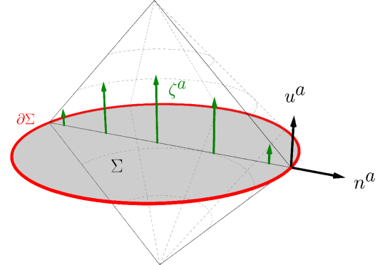
Figure 1: The causal diamond consists of the future and past domains of dependence of a spatial sphere $\Sigma$ in a MSS. $\Sigma$ has a unit normal $u^{a}$, induced metric $h_{ab}$, and volume form $\eta$. The boundary $\partial\Sigma$ has a spacelike unit normal $n^{a}$, defined to be orthogonal to $u^{a}$, and volume form $\mu$. The conformal Killing vector $\zeta^{a}$ generates a flow within the causal diamond, and vanishes on the bifurcation surface $\partial\Sigma$.

The Wald formalism contains ambiguities identified by Jacobson, Kang and Myers (JKM) [163] that modify the Wald entropy and the generalized volume by the terms $S_{\text{JKM}}$ and $W_{\text{JKM}}$ given in (42) and (43). Using a modified generalized volume defined by

$$W^{\prime}=W+W_{\text{JKM}}\,,$$ (4)

the identity (2) continues to hold with $\delta(S_{\text{Wald}}+S_{\text{JKM}})\big{|}_{W^{\prime}}$ replacing $\delta S_{\text{Wald}}\big{|}_{W}$ . As discussed in section 1, the subleading divergences for the entanglement entropy involve a particular resolution of the JKM ambiguity, while section 4 argues that the first law of causal diamond mechanics applies for any resolution, as long as the appropriate generalized volume is held fixed.

Using the resolution of the JKM ambiguity required for the entanglement entropy calculation, the first law leads to the following statement of entanglement equilibrium, applicable to higher curvature theories:

Hypothesis (Entanglement Equilibrium).

In a quantum gravitational theory, the entanglement entropy of a spherical region with fixed generalized volume $W^{\prime}$ is maximal in vacuum.

This modifies the original equilibrium condition (1) by replacing the area variation with

$$\delta(S_{\text{Wald}}+S_{\text{JKM}})\big{|}_{W^{\prime}}\,.$$ (5)

In Section 2.3, this equilibrium condition is shown to be equivalent to the linearized higher derivative field equations in the case that the matter fields are conformally invariant. Facts about entanglement entropy divergences and the reduced density matrix for a sphere in a CFT are used to relate the total variation of the entanglement entropy to the left hand side of (2). Once this is done, it becomes clear that imposing the linearized constraint equations is equivalent to the entanglement equilibrium condition.

In [121], this condition was applied in the small ball limit, in which any geometry looks like a perturbation of a MSS. Using Riemann normal coordinates (RNC), the linearized equations were shown to impose the fully nonlinear equations for the case of Einstein gravity. We will discuss this argument in Section 2.4 for higher curvature theories, and show that the nonlinear equations can not be obtained from the small ball limit, making general relativity unique in that regard.

In section 2.5, we discuss several implications of this work. First, we describe how it compares to other approaches connecting geometry and entanglement. Following that, we provide a possible thermodynamic interpretation of the first law of causal diamond mechanics derived in section 2.2. We then comment on a conjectural relation between our generalized volume $W$ and higher curvature holographic complexity. Finally, we lay out several future directions for the entanglement equilibrium program.

2.2 First law of causal diamond mechanics

Jacobson’s entanglement equilibrium argument [121] compares the surface area of a small spatial ball $\Sigma$ in a curved spacetime to the one that would be obtained in a MSS. The comparison is made using balls of equal volume $V$, a choice justified by an Iyer-Wald variational identity [64] for the conformal Killing vector $\zeta^{a}$ of the causal diamond in the maximally symmetric background. When the Einstein equation holds, this identity implies the first law of causal diamond mechanics [121, 167]

$$-\delta H_{\zeta}^{m}=\frac{\kappa}{8\pi G}\delta A-\frac{\kappa k}{8\pi G}\delta V\,,$$ (6)

where $k$ is the trace of the extrinsic curvature of $\partial\Sigma$ embedded in $\Sigma$, and the matter conformal Killing energy $H_{\zeta}^{m}$ is constructed from the stress tensor $T_{ab}$ by

$$H_{\zeta}^{m}=\int_{\Sigma}\eta\,u^{a}\zeta^{b}T_{ab}\,.$$ (7)

The purpose of this section is to generalize the variational identity to higher derivative theories, and to clarify its relation to the equations of motion. This is done by focusing on an off-shell version of the identity, which reduces to the first law when the linearized constraint equations for the theory are satisfied. We begin by reviewing the Iyer-Wald formalism in subsection 1, which also serves to establish notation. After describing the geometric setup in subsection 2, we show in subsection 3 how the quantities appearing in the identity can be written as variations of local geometric functionals of the surface $\Sigma$ and its boundary $\partial\Sigma$. As one might expect, the area is upgraded to the Wald entropy $S_{\text{Wald}}$, and we derive the generalization of the volume given in equation (3). Subsection 4 describes how the variational identity can instead be viewed as a variation at fixed generalized volume $W$, as quoted in equation (2), and describes the effect that JKM ambiguities have on the setup.

1 Iyer-Wald formalism

We begin by recalling the Iyer-Wald formalism [63, 64]. A general diffeomorphism invariant theory may be defined by its Lagrangian $L[\phi]$, a spacetime $d$-form locally constructed from the dynamical fields $\phi$, which include the metric and matter fields. A variation of this Lagrangian takes the form

$$\delta L=E\cdot\delta\phi+\mathrm{d}\theta[\delta\phi]\,,$$ (8)

where $E$ collectively denotes the equations of motion for the dynamical fields, and $\theta$ is the symplectic potential $(d-1)$-form. Taking an antisymmetric variation of $\theta$ yields the symplectic current $(d-1)$-form

$$\omega[\delta_{1}\phi,\delta_{2}\phi]=\delta_{1}\theta[\delta_{2}\phi]-\delta_{2}\theta[\delta_{1}\phi]\,,$$ (9)

whose integral over a Cauchy surface $\Sigma$ gives the symplectic form for the phase space description of the theory. Given an arbitrary vector field $\zeta^{a}$, evaluating the symplectic form on the Lie derivative $\pounds_{\zeta}\phi$ gives the variation of the Hamiltonian $H_{\zeta}$ that generates the flow of $\zeta^{a}$

$$\delta H_{\zeta}=\int_{\Sigma}\omega[\delta\phi,\pounds_{\zeta}\phi]\,.$$ (10)

Now consider a ball-shaped region $\Sigma$, and take $\zeta^{a}$ to be any future-pointed, timelike vector that vanishes on the boundary $\partial\Sigma$. Wald’s variational identity then reads

$$\int_{\Sigma}\omega[\delta\phi,\pounds_{\zeta}\phi]=\int_{\Sigma}\delta J_{\zeta}\,,$$ (11)

where the Noether current $J_{\zeta}$ is defined by

$$J_{\zeta}=\theta[\pounds_{\zeta}\phi]-i_{\zeta}L\,.$$ (12)

Here $i_{\zeta}$ denotes contraction of the vector $\zeta^{a}$ on the first index of the differential form $L$. The identity (11) holds when the background geometry satisfies the field equations $E=0$, and it assumes that $\zeta^{a}$ vanishes on $\partial\Sigma$. Next we note that the Noether current can always be expressed as [84]

$$J_{\zeta}=\mathrm{d}Q_{\zeta}+C_{\zeta},$$ (13)

where $Q_{\zeta}$ is the Noether charge $(d-2)$-form and $C_{\zeta}$ are the constraint field equations, which arise as a consequence of the diffeomorphism gauge symmetry. For non-scalar matter, these constraints are a combination of the metric and matter field equations [168, 169], but, assuming the matter equations are imposed, we can take

$$C_{\zeta}=-2\zeta^{a}E\indices{{}_{a}^{b}}\epsilon_{b},$$ (14)

where $E^{ab}$ is the variation of the Lagrangian density with respect to the metric. By combining equations (10), (11) and (13), one finds that

$$-\int_{\partial\Sigma}\delta Q_{\zeta}+\delta H_{\zeta}=\int_{\Sigma}\delta C_{\zeta}\,.$$ (15)

When the linearized constraints hold, $\delta C_{\zeta}=0$, the variation of the Hamiltonian is a boundary integral of $\delta Q_{\zeta}$. This on-shell identity forms the basis for deriving the first law of causal diamond mechanics. Unlike the situation encountered in black hole thermodynamics, $\delta H_{\zeta}$ is not zero because below we take $\zeta^{a}$ to be a conformal Killing vector as opposed to a true Killing vector.

2 Geometric setup

Thus far, the only restriction that has been placed on the vector field $\zeta^{a}$ is that it vanishes on $\partial\Sigma$. As such, the quantities $\delta H_{\zeta}$ and $\delta Q_{\zeta}$ appearing in the identities depend rather explicitly on the fixed vector $\zeta^{a}$, and therefore these quantities are not written in terms of only the geometric properties of the surfaces $\Sigma$ and $\partial\Sigma$. A purely geometric description is desirable if the Hamiltonian and Noether charge are to be interpreted as thermodynamic state functions, which ultimately may be used to define the ensemble of geometries in any proposed quantum description of the microstates. This situation may be remedied by choosing the vector $\zeta^{a}$ and the surface $\Sigma$ to have special properties in the background geometry. In particular, by choosing $\zeta^{a}$ to be a conformal Killing vector for a causal diamond in the MSS, and picking $\Sigma$ to lie on the surface where the conformal factor vanishes, one finds that the perturbations $\delta H_{\zeta}$ and $\delta Q_{\zeta}$ have expressions in terms of local geometric functionals on the surfaces $\Sigma$ and $\partial\Sigma$, respectively.

Given a causal diamond in a MSS, there exists a conformal Killing vector $\zeta^{a}$ which generates a flow within the diamond and vanishes at the bifurcation surface $\partial\Sigma$ (see figure 1). The metric satisfies the conformal Killing equation

$$\pounds_{\zeta}g_{ab}=2\alpha g_{ab}\quad\text{with}\quad\alpha=\frac{1}{d}\nabla_{c}\zeta^{c}\,.$$ (16)

and the conformal factor $\alpha$ vanishes on the spatial ball $\Sigma$. The gradient of $\alpha$ is hence proportional to the unit normal to $\Sigma$,

$$u_{a}=N\nabla_{a}\alpha\quad\text{with}\quad N=\lVert\nabla_{a}\alpha\rVert^{-1}.$$ (17)

Note the vector $u^{a}$ is future pointing since the conformal factor $\alpha$ decreases to the future of $\Sigma$. In a MSS, the normalization function $N$ has the curious property that it is constant over $\Sigma$, and is given by [167]

$$N=\frac{d-2}{\kappa k},$$ (18)

where $k$ is the trace of the extrinsic curvature of $\partial\Sigma$ embedded in $\Sigma$, and $\kappa$ is the surface gravity of the conformal Killing horizon, defined momentarily. This constancy ends up being crucial to finding a local geometric functional for $\delta H_{\zeta}$. Throughout this chapter, $N$ and $k$ will respectively denote constants equal to the normalization function and extrinsic curvature trace, both evaluated in the background spacetime.

Since $\alpha$ vanishes on $\Sigma$, $\zeta^{a}$ is instantaneously a Killing vector. On the other hand, the covariant derivative of $\alpha$ is nonzero, so

$$\nabla_{d}(\pounds_{\zeta}g_{ab})\big{|}_{\Sigma}=\frac{2}{N}u_{d}g_{ab}\,.$$ (19)

The fact that the covariant derivative is nonzero on $\Sigma$ is responsible for making $\delta H_{\zeta}$ nonvanishing.

A conformal Killing vector with a horizon has a well-defined surface gravity $\kappa$ [122], and since $\alpha$ vanishes on $\partial\Sigma$, we can conclude that

$$\nabla_{a}\zeta_{b}\big{|}_{\partial\Sigma}=\kappa n_{ab}\,,$$ (20)

where $n_{ab}=2u_{[a}n_{b]}$ is the binormal for the surface $\partial\Sigma$, and $n^{b}$ is the outward pointing spacelike unit normal to $\partial\Sigma$. Since $\partial\Sigma$ is a bifurcation surface of a conformal Killing horizon, $\kappa$ is constant everywhere on it. We provide an example of these constructions in appendix 2.A where we discuss the conformal Killing vector for a causal diamond in flat space.

3 Local geometric expressions

In this subsection we evaluate the Iyer-Wald identity (15) for an arbitrary higher derivative theory of gravity and for the geometric setup described above. The final on-shell result is given in (36), which is the first law of causal diamond mechanics for higher derivative gravity.

Throughout the computation we assume that the matter fields are minimally coupled, so that the Lagrangian splits into a metric and matter piece $L=L^{g}+L^{m}$, and we take $L^{g}$ to be an arbitrary, diffeomorphism-invariant function of the metric, Riemann tensor, and its covariant derivatives. The symplectic potential and variation of the Hamiltonian then exhibit a similar separation, $\theta=\theta^{g}+\theta^{m}$ and $\delta H_{\zeta}=\delta H_{\zeta}^{g}+\delta H_{\zeta}^{m}$, and so we can write equation (15) as

$$-\int_{\partial\Sigma}\delta Q_{\zeta}+\delta H_{\zeta}^{g}+\delta H_{\zeta}^{m}=\int_{\Sigma}\delta C_{\zeta}\,.$$ (21)

Below, we explicitly compute the two terms $\delta H_{\zeta}^{g}$ and $\int_{\partial\Sigma}\delta Q_{\zeta}$ for the present geometric context.

Wald entropy.

By virtue of equation (20) and the fact that $\zeta^{a}$ vanishes on $\partial\Sigma$, one can show that the integrated Noether charge is simply related to the Wald entropy [63, 64]

$$-\int_{\partial\Sigma}Q_{\zeta} =\int_{\partial\Sigma}\,E^{abcd}\,\epsilon_{ab}\nabla_{c}\zeta_{d}$$

$$=\frac{\kappa}{2\pi}S_{\text{Wald}}\,,$$ (22)

where the Wald entropy is defined as

$$S_{\text{Wald}}=-2\pi\int_{\partial\Sigma}\mu\,E^{abcd}n_{ab}n_{cd}\,.$$ (23)

$E^{abcd}$ is the variation of the Lagrangian scalar with respect to the Riemann tensor $R_{abcd}$ taken as an independent field, given in (69), and $\mu$ is the volume form on $\partial\Sigma$, so that $\epsilon_{ab}=-n_{ab}\wedge\mu$ there. The equality (22) continues to hold at first order in perturbations, which can be shown following the same arguments as given in [64], hence,

$$\int_{\partial\Sigma}\delta Q_{\zeta}=-\frac{\kappa}{2\pi}\delta S_{\text{Wald}}\,.$$ (24)

The minus sign is opposite the convention in [64] since the unit normal $n^{a}$ is outward pointing for the causal diamond.

Generalized volume.

The gravitational part of $\delta H_{\zeta}$ is related to the symplectic current $\omega[\delta g,\pounds_{\zeta}g]$ via (10). The symplectic form has been computed on an arbitrary background for any higher curvature gravitational theory whose Lagrangian is a function of the Riemann tensor, but not its covariant derivatives [170]. Here, we take advantage of the maximal symmetry of the background to compute the symplectic form and Hamiltonian for the causal diamond in any higher order theory, including those with derivatives of the Riemann tensor.

Recall that the symplectic current $\omega$ is defined in terms of the symplectic potential $\theta$ through (9). For a Lagrangian that depends on the Riemann tensor and its covariant derivatives, the symplectic potential $\theta^{g}$ is given in Lemma 3.1 of [64]

$$\theta^{g} =2E^{bcd}\nabla_{d}\delta g_{bc}+S^{ab}\delta g_{ab}$$

$$+\sum_{i=1}^{m-1}T_{i}^{abcda_{1}\ldots a_{i}}\delta\nabla_{(a_{1}}\cdots\nabla_{a_{i})}R_{abcd}\,,$$ (25)

where $E^{bcd}=\epsilon_{a}E^{abcd}$ and the tensors $S^{ab}$ and $T_{i}^{abcda_{1}\ldots a_{i}}$ are locally constructed from the metric, its curvature, and covariant derivatives of the curvature. Due to the antisymmetry of $E^{bcd}$ in $c$ and $d$, the symplectic current takes the form

$$\omega^{g}=2\delta_{1}E^{bcd}\nabla_{d}\delta_{2}g_{bc}-2E^{bcd}\delta_{1}\Gamma^{e}_{db}\delta_{2}g_{ec}+\delta_{1}S^{ab}\delta_{2}g_{ab}$$

$$+\sum_{i=1}^{m-1}\delta_{1}T_{i}^{abcda_{1}\ldots a_{i}}\delta_{2}\nabla_{(a_{1}}\cdots\nabla_{a_{i})}R_{abcd}-(1\leftrightarrow 2).$$ (26)

Next we specialize to the geometric setup described in section 2. We may thus employ the fact that we are perturbing around a maximally symmetric background. This means the background curvature tensor takes the form

$$R_{abcd}=\frac{R}{d(d-1)}(g_{ac}g_{bd}-g_{ad}g_{bc})$$ (27)

with a constant Ricci scalar $R$, so that $\nabla_{e}R_{abcd}=0$, and also $\pounds_{\zeta}R_{abcd}\big{|}_{\Sigma}=0$. Since the tensors $E^{abcd}$, $S^{ab}$, and $T_{i}^{abcda_{1}\ldots a_{i}}$ are all constructed from the metric and curvature, they will also have vanishing Lie derivative along $\zeta^{a}$ when evaluated on $\Sigma$.

Replacing $\delta_{2}g_{ab}$ in equation (26) with $\pounds_{\zeta}g_{ab}$ and using (19), we obtain

$$\omega^{g}[\delta g,\pounds_{\zeta}g]\big{|}_{\Sigma}=$$

$$\qquad\frac{2}{N}\left[2g_{bc}u_{d}\delta E^{bcd}+E^{bcd}(u_{d}\delta g_{bc}-g_{bd}u^{e}\delta g_{ec})\right].$$ (28)

We would like to write this as a variation of some scalar quantity. To do so, we split off the background value of $E^{abcd}$ by writing

$$F^{abcd}=E^{abcd}-E_{0}(g^{ac}g^{bd}-g^{ad}g^{bc})\,.$$ (29)

The second term in this expression is the background value, and, due to maximal symmetry, the scalar $E_{0}$ must be a constant determined by the parameters appearing in the Lagrangian. By definition, $F^{abcd}$ is zero in the background, so any term in (3) that depends on its variation may be immediately written as a total variation, since variations of other tensors appearing in the formula would multiply the background value of $F^{abcd}$, which vanishes. Hence, the piece involving $\delta F^{abcd}$ becomes

$$\frac{4}{N}g_{bc}u_{d}\delta(F^{abcd}\epsilon_{a})=\frac{4}{N}\delta(F^{abcd}g_{bc}u_{d}\epsilon_{a})\,.$$ (30)

The remaining terms simply involve replacing $E^{abcd}$ in (3) with $E_{0}(g^{ac}g^{bd}-g^{ad}g^{bc})$. These terms then take exactly the same form as the terms that appear for general relativity, which we know from the appendix of [121] combine to give an overall variation of the volume. The precise form of this variation when restricted to $\Sigma$ is

$$-\frac{4(d-2)}{N}\delta\eta\,,$$ (31)

where $\eta$ is the induced volume form on $\Sigma$. Adding this to (30) produces

$$\omega[\delta g,\pounds_{\zeta}g]\big{|}_{\Sigma}=-\frac{4}{N}\delta\left[\eta(E^{abcd}u_{a}u_{d}h_{bc}-E_{0})\right]\,,$$ (32)

where we used that $\epsilon_{a}=-u_{a}\wedge\eta$ on $\Sigma$. This leads us to define a generalized volume functional

$$W=\frac{1}{(d-2)E_{0}}\int_{\Sigma}{\eta}(E^{abcd}u_{a}u_{d}h_{bc}-E_{0})\,,$$ (33)

and the variation of this quantity is related to the variation of the gravitational Hamiltonian by

$$\delta H_{\zeta}^{g}=-4E_{0}\kappa k\,\delta W\,,$$ (34)

where we have expressed $N$ in terms of $\kappa$ and $k$ using (18). We have thus succeeded in writing $\delta H^{g}_{\zeta}$ in terms of a local geometric functional defined on the surface $\Sigma$.

It is worth emphasizing that $N$ being constant over the ball was crucial to this derivation, since otherwise it could not be pulled out of the integral over $\Sigma$ and would define a non-diffeomorphism invariant structure on the surface. Note that the overall normalization of $W$ is arbitrary, since a different normalization would simply change the coefficient in front of $\delta W$ in (34). As one can readily check, the normalization in (33) was chosen so that $W$ reduces to the volume in the case of Einstein gravity. In appendix 2.B we provide explicit expressions for the generalized volume in $f(R)$ gravity and quadratic gravity.

Finally, combining (24), (34) and (21), we arrive at the off-shell variational identity in terms of local geometric quantities

$$\frac{\kappa}{2\pi}\delta S_{\text{Wald}}-4E_{0}\kappa k\delta W+\delta H_{\zeta}^{m}=\int_{\Sigma}\delta C_{\zeta}\,.$$ (35)

By imposing the linearized constraints $\delta C_{\zeta}=0$, this becomes the first law of causal diamond mechanics for higher derivative gravity

$$-\delta H_{\zeta}^{m}=\frac{\kappa}{2\pi}\delta S_{\text{Wald}}-4E_{0}\kappa k\delta W\,.$$ (36)

This reproduces (6) for Einstein gravity with Lagrangian $L=\epsilon R/16\pi G$, for which $E_{0}=1/32\pi G$.

4 Variation at fixed $W$

We now show that the first two terms in (35) can be written in terms of the variation of the Wald entropy at fixed $W$, defined as

$$\delta S_{\text{Wald}}\big{|}_{W}=\delta S_{\text{Wald}}-\frac{\partial S_{\text{Wald}}}{\partial W}\delta W\,.$$ (37)

Here we must specify what is meant by $\frac{\partial S_{\text{Wald}}}{\partial W}$. We will take this partial derivative to refer to the changes that occur in both quantities when the size of the ball is deformed, but the metric and dynamical fields are held fixed. Take a vector $v^{a}$ that is everywhere tangent to $\Sigma$ that defines an infinitesimal change in the shape of $\Sigma$. The first order change this produces in $S_{\text{Wald}}$ and $W$ can be computed by holding $\Sigma$ fixed, but varying the Noether current and Noether charge as $\delta J_{\zeta}=\pounds_{v}J_{\zeta}$ and $\delta Q_{\zeta}=\pounds_{v}Q_{\zeta}$. Since the background field equations are satisfied and $\zeta^{a}$ vanishes on $\partial\Sigma$, we have there that $\int_{\partial\Sigma}Q_{\zeta}=\int_{\Sigma}J_{\zeta}^{g}$, without reference to the matter part of the Noether current. Recall that $\delta W$ is related to the variation of the gravitational Hamiltonian, which can be expressed in terms of $\delta J^{g}_{\zeta}$ through (10) and (11). Then using the relations (22) and (34) and the fact that the Lie derivative commutes with the exterior derivative, we may compute

$$\frac{\partial S_{\text{Wald}}}{\partial W}=\frac{-\frac{2\pi}{\kappa}\int_{\partial\Sigma}\pounds_{v}Q_{\zeta}}{-\frac{1}{4E_{0}\kappa k}\int_{\Sigma}\pounds_{v}J_{\zeta}^{g}}=8\pi E_{0}k\,.$$ (38)

Combining this result with equations (36) and (37) we arrive at the off-shell variational identity for higher derivative gravity quoted in the introduction

$$\frac{\kappa}{2\pi}\delta S_{\text{Wald}}\big{|}_{W}+\delta H_{\zeta}^{m}=\int_{\Sigma}\delta C_{\zeta}\,.$$ (39)

Finally, we comment on how JKM ambiguities [163] affect this identity. The particular ambiguity we are concerned with comes from the fact that the symplectic potential $\theta$ in equation (8) is defined only up to addition of an exact form $\mathrm{d}Y[\delta\phi]$ that is linear in the field variations and their derivatives. This has the effect of changing the Noether current and Noether charge by

$$J_{\zeta} \rightarrow J_{\zeta}+\mathrm{d}Y[\pounds_{\zeta}\phi]\,,$$ (40)

$$Q_{\zeta} \rightarrow Q_{\zeta}+Y[\pounds_{\zeta}\phi]\,.$$ (41)

This modifies both the entropy and the generalized volume by surface terms on $\partial\Sigma$ given by

$$S_{\text{JKM}} =-\frac{2\pi}{\kappa}\int_{\partial\Sigma}Y[\pounds_{\zeta}\phi]\,,$$ (42)

$$W_{\text{JKM}} =-\frac{1}{4E_{0}\kappa k}\int_{\partial\Sigma}Y[\pounds_{\zeta}\phi]\,.$$ (43)

However, it is clear that this combined change in $J_{\zeta}$ and $Q_{\zeta}$ leaves the left hand side of (39) unchanged, since the $Y$-dependent terms cancel out. In particular,

$$\delta S_{\text{Wald}}\big{|}_{W}=\delta(S_{\text{Wald}}+S_{\text{JKM}})\big{|}_{W+W_{\text{JKM}}}\,,$$ (44)

showing that any resolution of the JKM ambiguity gives the same first law, provided that the Wald entropy and generalized volume are modified by the terms (42) and (43). This should be expected, because the right hand side of (39) depends only on the field equations, which are unaffected by JKM ambiguities.

2.3 Entanglement Equilibrium

The original entanglement equilibrium argument for Einstein gravity stated that the total variation away from the vacuum of the entanglement of a region at fixed volume is zero. This statement is encapsulated in equation (1), which shows both an area variation due to the change in geometry, and a matter piece from varying the quantum state. The area variation at fixed volume can equivalently be written

$$\delta A\big{|}_{V}=\delta A-\frac{\partial A}{\partial V}\delta V$$ (45)

and the arguments of section 4 relate this combination to the terms appearing in the first law of causal diamond mechanics (6). Since $\delta H_{\zeta}^{m}$ in (6) is related to $\delta S_{\text{mat}}$ in (1) for conformally invariant matter, the first law may be interpreted entirely in terms of entanglement entropy variations.

This section discusses the extension of the argument to higher derivative theories of gravity. Subsection 1 explains how subleading divergences in the entanglement entropy are related to a Wald entropy, modified by a particular resolution of the JKM ambiguity. Paralleling the Einstein gravity derivation, we seek to relate variations of the subleading divergences to the higher derivative first law of causal diamond mechanics (36). Subsection 2 shows that this can be done as long as the generalized volume $W^{\prime}$ [related to $W$ by a boundary JKM term as in (4)] is held fixed. Then, using the relation of the first law to the off-shell identity (39), we discuss how the entanglement equilibrium condition is equivalent to imposing the linearized constraint equations.

1 Subleading entanglement entropy divergences

As discussed in section 3, the subleading divergences in the entanglement entropy are given by a local integral over the entangling surface. When the entangling surface is the bifurcation surface of a stationary horizon, this local integral is simply the Wald entropy [85, 84]. On nonstationary entangling surfaces, the computation can be done using the squashed cone techniques of [171], which yield terms involving extrinsic curvatures that modify the Wald entropy. In holography, the squashed cone method plays a key role in the proof of the Ryu-Takayanagi formula [104, 172], and its higher curvature generalization [164, 173]. The entropy functionals obtained in these works seem to also apply outside of holography, giving the extrinsic curvature terms in the entanglement entropy for general theories [171, 83].

The extrinsic curvature modifications to the Wald entropy in fact take the form of a JKM Noether charge ambiguity [163, 177, 178]. To see this, note the vector $\zeta^{a}$ used to define the Noether charge vanishes at the entangling surface and its covariant derivative is antisymmetric and proportional to the binormal as in equation (20). This means it acts like a boost on the normal bundle at the entangling surface. General covariance requires that any extrinsic curvature contributions can be written as a sum of boost-invariant products,

$$S_{\text{JKM}}=\int_{\partial\Sigma}\mu\sum_{n\geq 1}B^{(-n)}\cdot C^{(n)}$$ (46)

where the superscript $(n)$ denotes the boost weight of that tensor, so that at the surface: $\pounds_{\zeta}C^{(n)}=nC^{(n)}$. It is necessary that the terms consist of two pieces, each of which has nonzero boost weight, so that they can be written as

$$S_{\text{JKM}}=\int_{\partial\Sigma}\mu\sum_{n\geq 1}\frac{1}{n}B^{(-n)}\cdot\pounds_{\zeta}C^{(n)}\,.$$ (47)

This is of the form of a Noether charge ambiguity from equation (41), with

$$Y[\delta\phi]=\mu\sum_{n\geq 1}\frac{1}{n}B^{(-n)}\delta C^{(n)}\,.$$ (48)

The upshot of this discussion is that all terms in the entanglement entropy that are local on the entangling surface, including all divergences, are given by a Wald entropy modified by specific JKM terms. The couplings for the Wald entropy are determined by matching to the UV completion, or, in the absence of the UV description, these are simply parameters characterizing the low energy effective theory. In induced gravity scenarios, the divergences are determined by the matter content of the theory, and the matching to gravitational couplings has been borne out in explicit examples [179, 180, 181].

2 Equilibrium condition as gravitational constraints

We can now relate the variational identity (39) to entanglement entropy. The reduced density matrix for the ball in vacuum takes the form

$$\rho_{\Sigma}=e^{-H_{\text{mod}}}/Z\,,$$ (49)

where $H_{\text{mod}}$ is the modular Hamiltonian and $Z$ is the partition function, ensuring that $\rho_{\Sigma}$ is normalized. Since the matter is conformally invariant, the modular Hamiltonian takes a simple form in terms of the matter Hamiltonian $H_{\zeta}^{m}$ defined in (7) [142, 143]

$$H_{\text{mod}}=\frac{2\pi}{\kappa}H_{\zeta}^{m}\,.$$ (50)

Next we apply the first law of entanglement entropy [124, 123], which states that the first order perturbation to the entanglement entropy is given by the change in modular Hamiltonian expectation value

$$\delta S_{\text{EE}}=\delta\langle H_{\text{mod}}\rangle\,.$$ (51)

Note that this equation holds for a fixed geometry and entangling surface, and hence coincides with what was referred to as $\delta S_{\text{mat}}$ in section 2.1. When varying the geometry, the divergent part of the entanglement entropy changes due to a change in the Wald entropy and JKM terms of the entangling surface. The total variation of the entanglement entropy is therefore

$$\delta S_{\text{EE}}=\delta(S_{\text{Wald}}+S_{\text{JKM}})+\delta\langle H_{\text{mod}}\rangle\,.$$ (52)

At this point, we must give a prescription for defining the surface $\Sigma$ in the perturbed geometry. Motivated by the first law of causal diamond mechanics, we require that $\Sigma$ has the same generalized volume $W^{\prime}$ as in vacuum, where $W^{\prime}$ differs from the quantity $W$ by a JKM term, as in equation (4). This provides a diffeomorphism-invariant criterion for defining the overall radius of the ball, since this radius may be adjusted until the generalized volume $W^{\prime}$ is equal to its vacuum value. It does not fully fix all properties of the surface, but it is enough to derive the equilibrium condition for the entropy. As argued in section 4, the first term in equation (52) can be written instead as $\delta S_{\text{Wald}}\big{|}_{W}$ when the variation is taken holding $W^{\prime}$ fixed. Thus, from equations (39), (50) and (52), we arrive at our main result, the equilibrium condition

$$\frac{\kappa}{2\pi}\delta S_{\text{EE}}\big{|}_{W^{\prime}}=\int_{\Sigma}\delta C_{\zeta}\,,$$ (53)

valid for minimally coupled, conformally invariant matter fields.

The linearized constraint equations $\delta C_{\zeta}=0$ may therefore be interpreted as an equilibrium condition on entanglement entropy for the vacuum. Since all first variations of the entropy vanish when the linearized gravitational constraints are satisfied, the vacuum is an extremum of entropy for regions with fixed generalized volume $W^{\prime}$, which is necessary for it to be an equilibrium state. Alternatively, postulating that entanglement entropy is maximal in vacuum for all balls and in all frames would allow one to conclude that the linearized higher derivative equations hold everywhere.

2.4 Field equations from the equilibrium condition

The entanglement equilibrium hypothesis provides a clear connection between the linearized gravitational constraints and the maximality of entanglement entropy at fixed $W^{\prime}$ in the vacuum for conformally invariant matter. In this section, we will consider whether information about the fully nonlinear field equations can be gleaned from the equilibrium condition. Following the approach taken in [121], we employ a limit where the ball is taken to be much smaller than all relevant scales in the problem, but much larger than the cutoff scale of the effective field theory, which is set by the gravitational coupling constants. By expressing the linearized equations in Riemann normal coordinates, one can infer that the full nonlinear field equations hold in the case of Einstein gravity. As we discuss here, such a conclusion can not be reached for higher curvature theories. The main issue is that higher order terms in the RNC expansion are needed to capture the effect of higher curvature terms in the field equations, but these contribute at the same order as nonlinear corrections to the linearized equations.

We begin by reviewing the argument for Einstein gravity. Near any given point, the metric looks locally flat, and has an expansion in terms of Riemann normal coordinates that takes the form

$$g_{ab}(x)=\eta_{ab}-\frac{1}{3}x^{c}x^{d}R_{acbd}(0)+\mathcal{O}(x^{3})\,,$$ (54)

where $(0)$ means evaluation at the center of the ball. At distances small compared to the radius of curvature, the second term in this expression is a small perturbation to the flat space metric $\eta_{ab}$. Hence, we may apply the off-shell identity (53), using the first order variation

$$\delta g_{ab}=-\frac{1}{3}x^{c}x^{d}R_{acbd}(0)\,,$$ (55)

and conclude that the linearized constraint $\delta C_{\zeta}$ holds for this metric perturbation. When restricted to the surface $\Sigma$, this constraint in Einstein gravity is [168]

$$C_{\zeta}\big{|}_{\Sigma}=-u^{a}\zeta^{b}\left(\frac{1}{8\pi G}G_{ab}-T_{ab}\right)\eta\,.$$ (56)

Since the background constraint is assumed to hold, the perturbed constraint is

$$\delta C_{\zeta}\big{|}_{\Sigma}=-u^{a}\zeta^{b}\left(\frac{1}{8\pi G}\delta G_{ab}-\delta T_{ab}\right)\eta\,,$$ (57)

but in Riemann normal coordinates, we have that the linearized perturbation to the curvature is just $\delta G_{ab}=G_{ab}(0)$, up to terms suppressed by the ball radius. Assuming that the ball is small enough so that the stress tensor may be taken constant over the ball, one concludes that the vanishing constraint implies the nonlinear field equation at the center of the ball

$$u^{a}\zeta^{b}(G_{ab}(0)-8\pi G\delta T_{ab})=0\,.$$ (58)

The procedure outlined above applies at all points and all frames, allowing us to obtain the full tensorial Einstein equation.

Since we have only been dealing with the linearized constraint, one could question whether it gives a good approximation to the field equations at all points within the small ball. This requires estimating the size of the nonlinear corrections to this field equation. When integrated over the ball, the corrections to the curvature in RNC are of order $\ell^{2}/L^{2}$, where $\ell$ is the radius of the ball and $L$ is the radius of curvature. Since we took the ball size to be much smaller than the radius of curvature, these terms are already suppressed relative to the linear order terms in the field equation.

The situation in higher derivative theories of gravity is much different. It is no longer the case that the linearized equations evaluated in RNC imply the full nonlinear field equations in a small ball. To see this, consider an $L[g_{ab},R_{bcde}]$ higher curvature theory. The equations of motion read

$$-\frac{1}{2}g^{ab}\mathcal{L}+E^{aecd}\tensor{R}{{}^{b}_{ecd}}-2\nabla_{c}\nabla_{d}E^{acdb}=\frac{1}{2}T^{ab}\,.$$ (59)

In appendix 2.C we show that linearizing these equations around a Minkowski background leads to

$$\frac{\delta G^{ab}}{16\pi G}-2\partial_{c}\partial_{d}\delta E^{acdb}_{\text{higher}}=\frac{1}{2}\delta T^{ab}\,,$$ (60)

where we split $E^{abcd}=E^{abcd}_{\text{Ein}}+E^{abcd}_{\text{higher}}$ into its Einstein piece, which gives rise to the Einstein tensor, and a piece coming from higher derivative terms. As noted before, the variation of the Einstein tensor evaluated in RNC gives the nonlinear Einstein tensor, up to corrections that are suppressed by the ratio of the ball size to the radius of curvature. However, in a higher curvature theory of gravity, the equations of motion (59) contain terms that are nonlinear in the curvature. Linearization around a MSS background of these terms would produce, schematically, $\delta(R^{n})=n\bar{R}^{n-1}\delta R$, where $\bar{R}$ denotes evaluation in the MSS background. In Minkowski space, all such terms would vanish. This is not true in a general MSS, but evaluating the curvature tensors in the background still leads to a significant loss of information about the tensor structure of the equation. We conclude that the linearized equations cannot reproduce the full nonlinear field equations for higher curvature gravity, and it is only the linearity of the Einstein equation in the curvature that allows the nonlinear equations to be obtained for general relativity.

When linearizing around flat space, the higher curvature corrections to the Einstein equation are entirely captured by the second term in (60), which features four derivatives acting on the metric, since $E_{\text{higher}}^{abcd}$ is constructed from curvatures that already contain two derivatives of the metric. Therefore, one is insensitive to higher curvature corrections unless at least $\mathcal{O}(x^{4})$ corrections [182] are added to the Riemann normal coordinates expansion (55)

$$\delta g^{(2)}_{ab}=x^{c}x^{d}x^{e}x^{f}\bigg{(}\frac{2}{45}R\indices{{}_{a}{}_{c}{}_{d}^{g}}R\indices{{}_{b}{}_{e}{}_{f}{}_{g}}-\frac{1}{20}\nabla_{c}\nabla_{d}R_{aebf}\bigg{)}\,.$$ (61)

Being quadratic in the Riemann tensor, this term contributes at the same order as the nonlinear corrections to the linearized field equations. Hence, linearization based on the RNC expansion up to $x^{4}$ terms is not fully self-consistent. This affirms the claim that for higher curvature theories, the nonlinear equations at a point cannot be derived by only imposing the linearized equations.

2.5 Discussion

Maximal entanglement of the vacuum state was proposed in [121] as a new principle in quantum gravity. It hinges on the assumption that divergences in the entanglement entropy are cut off at short distances, so it is ultimately a statement about the UV complete quantum gravity theory. However, the principle can be phrased in terms of the generalized entropy, which is intrinsically UV finite and well-defined within the low energy effective theory. Therefore, if true, maximal vacuum entanglement provides a low energy constraint on any putative UV completion of a gravitational effective theory.

Higher curvature terms arise generically in any such effective field theory. Thus, it is important to understand how the entanglement equilibrium argument is modified by them. As explained in section 2.2, the precise characterization of the entanglement equilibrium hypothesis relies on a classical variational identity for causal diamonds in maximally symmetric spacetimes. This identity leads to equation (39), which relates variations of the Wald entropy and matter energy density of the ball to the linearized constraints. The variations are taken holding fixed a new geometric functional $W$, defined in (33), which we call the “generalized volume.”

We connected this identity to entanglement equilibrium in section 2.3, invoking the fact that subleading entanglement entropy divergences are given by a Wald entropy, modified by specific JKM terms, which also modify $W$ by the boundary term (43). With the additional assumption that matter is conformally invariant, we arrived at our main result (53), showing that the equilibrium condition $\delta S_{\text{EE}}\big{|}_{W^{\prime}}=0$ applied to small balls is equivalent to imposing the linearized constraints $\delta C_{\zeta}=0$.

In section 2.4, we reviewed the argument that in the special case of Einstein gravity, imposing the linearized equations within small enough balls is equivalent to requiring that the fully nonlinear equations hold within the ball [121]. Thus by considering spheres centered at each point and in all Lorentz frames, one could conclude that the full Einstein equations hold everywhere. Such an argument cannot be made for a theory that involves higher curvature terms. One finds that higher order terms in the RNC expansion are needed to detect the higher curvature pieces of the field equations, but these terms enter at the same order as the nonlinear corrections to the linearized equations. This signals a breakdown of the perturbative expansion unless the curvature is small.

The fact that we obtain only linearized equations for the higher curvature theory is consistent with the effective field theory standpoint. One could take the viewpoint that higher curvature corrections are suppressed by powers of a UV scale, and the effective field theory is valid only when the curvature is small compared to this scale. This suppression would suggest that the linearized equations largely capture the effects of the higher curvature corrections in the regime where effective field theory is reliable.

1 Comparison to other “geometry from entanglement” approaches

Several proposals have been put forward to understand gravitational dynamics in terms of thermodynamics and entanglement. Here we will compare the entanglement equilibrium program considered in this chapter to two other approaches: the equation of state for local causal horizons, and gravitational dynamics from holographic entanglement entropy (see [134] for a related discussion).

Causal horizon equation of state

By assigning an entropy proportional to the area of local causal horizons, Jacobson showed that the Einstein equation arises as an equation of state [112]. This approach employs a physical process first law for the local causal horizon, defining a heat $\delta Q$ as the flux of local boost energy across the horizon. By assigning an entropy $S$ to the horizon proportional to its area, one finds that the Clausius relation $\delta Q=T\delta S$ applied to all such horizons is equivalent to the Einstein equation.

The entanglement equilibrium approach differs in that it employs an equilibrium state first law [equation (36)], instead of a physical process one [183]. It therefore represents a different perspective that focuses on the steady-state behavior, as opposed to dynamics involved with evolution along the causal horizon. It is consistent therefore that we obtain constraint equations in the entanglement equilibrium setup, since one would not expect evolution equations to arise as an equilibrium condition. That we can infer dynamical equations from the constraints is related to the fact that the dynamics of diffeomorphism-invariant theories is entirely determined by the constraints evaluated in all possible Lorentz frames.

Another difference comes from the focus on spacelike balls as opposed to local causal horizons. Dealing with a compact spatial region has the advantage of providing an IR finite entanglement entropy, whereas the entanglement associated with local causal horizons can depend on fields far away from the point of interest. This allows us to give a clear physical interpretation for the surface entropy functional as entanglement entropy, whereas such an interpretation is less precise in the equation of state approaches.

Finally, we note that both approaches attempt to obtain fully nonlinear equations by considering ultralocal regions of spacetime. In both cases the derivation of the field equations for Einstein gravity is fairly robust, however higher curvature corrections present some problems. Attempts have been made in the local causal horizon approach that involve modifying the entropy density functional for the horizon [184, 185, 186, 187, 188, 189, 190, 191, 192], but they meet certain challenges. These include a need for a physical interpretation of the chosen entropy density functional, and dependence of the entropy on arbitrary features of the local Killing vector in the vicinity of the horizon [192, 193]. While the entanglement equilibrium argument avoids these problems, it fails to get beyond linearized higher curvature equations, even after considering the small ball limit. The nonlinear equations in this case appear to involve information beyond first order perturbations, and hence may not be accessible based purely on an equilibrium argument.

Holographic entanglement entropy

A different approach comes from holography and the Ryu-Takayanagi formula [104]. By demanding that areas of minimal surfaces in the bulk match the entanglement entropies of spherical regions in the boundary CFT, one can show that the linearized gravitational equations must hold [115, 116, 117]. The argument employs an equilibrium state first law for the bulk geometry, utilizing the Killing symmetry associated with Rindler wedges in the bulk.

The holographic approach is quite similar to the entanglement equilibrium argument since both use equilibrium state first laws. One difference is that the holographic argument must utilize minimal surfaces in the bulk, which extend all the way to the boundary of AdS. This precludes using a small ball limit as can be done with the entanglement equilibrium derivation, and is the underlying reason that entanglement equilibrium can derive fully nonlinear field equations in the case of Einstein gravity, whereas the holographic approach has thus far only obtained linearized equations. Progress has been made to going beyond linear order in the holographic approach by considering higher order perturbations in the bulk [139, 194, 195, 118, 119]. Also, by considering the equality of bulk and boundary modular flow, the linearized argument in holography has been extended to applying in an arbitrary background [120], which suggests that a fully nonlinear derivation of the dynamics from entanglement can be obtained by integrating the linearized result.

2 Thermodynamic interpretation of the first law of causal diamond mechanics

Apart from the entanglement equilibrium interpretation, the first law of causal diamond mechanics could also directly be interpreted as a thermodynamic relation. Note that the identity (6) for Einstein gravity bears a striking resemblance to the fundamental relation in thermodynamics

$$dU=TdS-pdV,$$ (62)

where $U(S,V)$ is the internal energy, which is a function of the entropy $S$ and volume $V$. The first law (6) turns into the thermodynamic relation (62), if one makes the following identifications for the temperature $T$ and pressure $p$

$$T=\frac{\kappa\hbar}{2\pi k_{B}c}\,,\quad\quad p=\frac{c^{2}\kappa k}{8\pi G}\,.$$ (63)

Here we have restored fundamental constants, so that the quantities on the RHS have the standard units of temperature and pressure. The expression for the temperature is the well-known Unruh temperature [196]. The formula for the pressure lacks a microscopic understanding at the moment, although we emphasize the expression follows from consistency of the first law.

The thermodynamic interpretation motivates the name “first law” assigned to (6), and arguably it justifies the terminology “generalized volume” used for $W$ in this chapter, since it enters into the first law for higher curvature gravity (36) in the place of the volume. The only difference with the fundamental relation in thermodynamics is the minus sign in front of the energy variation. This different sign also enters into the first law for de Sitter horizons [197]. In the latter case the sign appears because empty de Sitter spacetime has maximal entropy, and adding matter only decreases the horizon entropy. Causal diamonds are rather similar in that respect.

3 Generalized volume and holographic complexity

The emergence of a generalized notion of volume in this analysis is interesting in its own right. We showed that when perturbing around a maximally symmetric background, the variation of the generalized volume is proportional to the variation of the gravitational part of the Hamiltonian. The fact that the Hamiltonian could be written in terms of a local, geometric functional of the surface was a nontrivial consequence of the background geometry being maximally symmetric and $\zeta^{a}$ being a conformal Killing vector whose conformal factor vanishes on $\Sigma$. The local geometric nature of $W$ makes it a useful, diffeomorphism invariant quantity with which to characterize the region under consideration, and thus should be a good state function in the thermodynamic description of an ensemble of quantum geometry microstates. One might hope that such a microscopic description would also justify the fixed-$W^{\prime}$ constraint in the entanglement equilibrium derivation, which was only motivated macroscopically by the first law of causal diamond mechanics.

Volume has recently been identified as an important quantity in holography, where it is conjectured to be related to complexity [198, 199], or fidelity susceptibility [200]. The complexity$=$volume conjecture states that the complexity of some boundary state on a time slice $\Omega$ is proportional to the volume of the extremal codimension-one bulk hypersurface $\mathcal{B}$ which meets the asymptotic boundary on the corresponding time slice.

While volume is the natural functional to consider for Einstein gravity, [201] noted that this should be generalized for higher curvature theories. The functional proposed in that work resembles our generalized volume $W$, but suffers from an arbitrary dependence on the choice of foliation of the codimension-one hypersurface on which it is evaluated. We therefore suggest that $W$, as defined in (33), may provide a suitable generalization of volume in the context of higher curvature holographic complexity.

Observe however that our derivation of $W$ using the Iyer-Wald formalism was carried out in the particular case of spherical regions whose causal diamond is preserved by a conformal Killing vector. On more general grounds, one could speculate that the holographic complexity functional in higher derivative gravities should involve contractions of $E^{abcd}$ with the geometric quantities characterizing $\mathcal{B}$, namely the induced metric $h_{ab}$ and the normal vector $u^{a}$. The most general functional involving at most one factor of $E^{abcd}$ can be written as

$$\mathcal{W}(\mathcal{B})=\int_{\mathcal{B}}\eta\left(\alpha E^{abcd}u_{a}h_{bc}u_{d}+\beta E^{abcd}h_{ad}h_{bc}+\gamma\right)\,,$$ (64)

for some constants $\alpha$, $\beta$ and $\gamma$ which should be such that $\mathcal{W}(\mathcal{B})=V(\mathcal{B})$ for Einstein gravity. It would be interesting to explore the validity of this proposal in particular holographic setups, e.g., along the lines of [204].

4 Future work

We conclude by laying out future directions for the entanglement equilibrium program.

Higher order perturbations

In this chapter we restricted attention only to first order perturbations of the entanglement entropy and the geometry. Working to higher order in perturbation theory could yield several interesting results. One such possibility would be proving that the vacuum entanglement entropy is maximal, as opposed to merely extremal. The second order change in entanglement entropy is no longer just the change in modular Hamiltonian expectation value. The difference is given by the relative entropy, so a proof of maximality will likely invoke the positivity of relative entropy. On the geometrical side, a second order variational identity would need to be derived, along the lines of [205]. One would expect that graviton contributions would appear at this order, and it would be interesting to examine how they play into the entanglement equilibrium story. Some initial steps towards such a derivation are taken in [206]. Also, by considering small balls and using the higher order terms in the Riemann normal coordinate expansion (61), in addition to higher order perturbations, it is possible that one could derive the fully nonlinear field equations of any higher curvature theory. Finally, coherent states pose a puzzle for the entanglement equilibrium hypothesis, since they change the energy within the ball without changing the entanglement [161]. However, their effect on the energy density only appears at second order in perturbations, so carrying the entanglement equilibrium argument to higher order could shed light on this puzzle.

Nonminimal couplings and gauge fields

We restricted attention to minimally coupled matter throughout this chapter. Allowing for nonminimal coupling can lead to new, state-dependent divergences in the entanglement entropy [207]. As before, these divergences will be localized on the entangling surface, taking the form of a Wald entropy. It therefore seems plausible that an entanglement equilibrium argument will go through in this case, reproducing the field equations involving the nonminimally coupled field. Note the state-dependent divergences could lead to variations of the couplings in the higher curvature theory, which may connect to the entanglement chemistry program, which considers Iyer-Wald first laws involving variations of the couplings [208].

Gauge fields introduce additional subtleties related to the existence of edge modes [125, 126, 127], and since these affect the renormalization of the gravitational couplings, they require special attention. Gravitons are even more problematic due to difficulties in defining the entangling surface in a diffeomorphism-invariant manner and in finding a covariant regulator [209, 88, 210, 83]. It would be interesting to analyze how to handle these issues in the entanglement equilibrium argument.

Nonspherical subregions

The entanglement equilibrium condition was shown to hold for spherical subregions and conformally invariant matter. One question that arises is whether an analogous equilibrium statement holds for linear perturbations to the vacuum in an arbitrarily shaped region. Nonspherical regions present a challenge because there is no longer a simple relation between the modular Hamiltonian and the matter stress tensor. Furthermore, nonspherical regions do not admit a conformal Killing vector which preserves its causal development. Since many properties of the conformal Killing vector were used when deriving the generalized volume $W$, it may need to be modified to apply to nonspherical regions and their perturbations.

Adapting the entanglement equilibrium arguments to nonspherical regions may involve shifting the focus to evolution under the modular flow, as opposed to a geometrical evolution generated by a vector field. Modular flows are complicated in general, but one may be able to use general properties of the flow to determine whether the Einstein equations still imply maximality of the vacuum entanglement for the region. Understanding the modular flow may also shed light on the behavior of the entanglement entropy for nonconformal matter, and whether some version of the entanglement equilibrium hypothesis continues to hold.

Physical process

As emphasized above, the first law of causal diamond mechanics is an equilibrium state construction since it compares the entropy of $\partial\Sigma$ on two infinitesimally related geometries [183]. One could ask whether there exists a physical process version of this story, which deals with entropy changes and energy fluxes as you evolve along the null boundary of the causal diamond. For this, the notion of quantum expansion for the null surface introduced in [83] would be a useful concept, which is defined by the derivative of the generalized entropy along the generators of the surface. One possible subtlety in formulating a physical process first law for the causal diamond is that the (classical) expansion of the null boundary is nonvanishing, so it would appear that this setup does not correspond to a dynamical equilibrium configuration. Nevertheless, it may be possible to gain useful information about the dynamics of semiclassical gravity by considering these nonequilibrium physical processes. An alternative that avoids this issue is to focus on quantum extremal surfaces [93] whose quantum expansion vanishes, and therefore may lend themselves to an equilibrium physical process first law.

Appendices

2.A Conformal Killing vector in flat space

Here we make explicit the geometric quantities introduced in section 2 in the case of a Minkowski background, whose metric we write in spherical coordinates, i.e., $ds^{2}=-dt^{2}+dr^{2}+r^{2}d\Omega_{d-2}^{2}$. Let $\Sigma$ be a spatial ball of radius $\ell$ in the time slice $t=0$ and with center at $r=0$. The conformal Killing vector which preserves the causal diamond of $\Sigma$ is given by [121]

$$\zeta=\left(\frac{\ell^{2}-r^{2}-t^{2}}{\ell^{2}}\right)\partial_{t}-\frac{2rt}{\ell^{2}}\partial_{r}\,,$$ (65)

where we have chosen the normalization in a way such that $\zeta^{2}=-1$ at the center of the ball, which then gives the usual notion of energy for $H_{\zeta}^{m}$ (i.e. the correct units). It is straightforward to check that $\zeta(t=\pm\ell,r=0)=\zeta(t=0,r=\ell)=0\,,$ i.e., the tips of the causal diamond and the maximal sphere $\partial\Sigma$ at its waist are fixed points of $\zeta$, as expected. Similarly, $\zeta$ is null on the boundary of the diamond. In particular, $\zeta(t=\ell\pm r)=\mp 2r(\ell\pm r)/\ell^{2}\cdot(\partial_{t}\pm\partial_{r})\,.$ The vectors $u$ and $n$ (respectively normal to $\Sigma$ and to both $\Sigma$ and $\partial\Sigma$) read $u=\partial_{t}$, $n=\partial_{r}$, so that the binormal to $\partial\Sigma$ is given by $n_{ab}=2\nabla_{[a}r\nabla_{b]}t\,.$ It is also easy to check that $\pounds_{\zeta}g_{ab}=2\alpha g_{ab}$ holds, where $\alpha\equiv\nabla_{a}\zeta^{a}/d=-2t/\ell^{2}\,.$ Hence, we immediately see that $\alpha=0$ on $\Sigma$, which implies that the gradient of $\alpha$ is proportional to the unit normal $u_{a}=-\nabla_{a}t$. Indeed, one finds $\nabla_{a}\alpha=-2\nabla_{a}t/\ell^{2}$, so in this case $N\equiv\lVert\nabla_{a}\alpha\rVert^{-1}=\ell^{2}/2$. It is also easy to show that $(\nabla_{a}\zeta_{b})|_{\partial\Sigma}=\kappa n_{ab}$ holds, where the surface gravity reads $\kappa=2/\ell$.

As shown in [122], given some metric $g_{ab}$ with a conformal Killing field $\zeta^{a}$, it is possible to construct other metrics $\bar{g}_{ab}$ conformally related to it, for which $\zeta^{a}$ is a true Killing field. More explicitly, if $\pounds_{\zeta}g_{ab}=2\alpha g_{ab}$, then $\pounds_{\zeta}\bar{g}_{ab}=0$ as long as $g_{ab}$ and $\bar{g}_{ab}$ are related through $\bar{g}_{ab}=\Phi\,g_{ab}$, where $\Phi$ satisfies

$$\pounds_{\zeta}\Phi+2\alpha\Phi=0\,.$$ (66)

For the vector (65), this equation has the general solution

$$\Phi(r,t)=\frac{\psi(s)}{r^{2}}\,\quad\text{where}\quad s\equiv\frac{\ell^{2}+r^{2}-t^{2}}{r}\,.$$ (67)

Here, $\psi(s)$ can be any function. Hence, $\zeta$ in (65) is a true Killing vector for all metrics conformally related to Minkowski’s with a conformal factor given by (67). For example, setting $\psi(s)=L^{2}$, for some constant $L^{2}$, one obtains the metric of AdS${}_{2}\times S_{d-2}$ with equal radii, namely: $ds^{2}=L^{2}/r^{2}(-dt^{2}+dr^{2})+L^{2}d\Omega_{d-2}^{2}$. Another simple case corresponds to $\psi(s)=L^{2}((s^{2}/(4L^{2})-1)^{-1}$. Through the change of variables [143]: $t=L\sinh(\tau/L)/(\cosh u+\cosh(\tau/L))$, $r=L\sinh u\,/(\cosh u+\cosh(\tau/L))$, this choice leads to the $\mathbb{R}\times H^{d-1}$ metric (where $H^{d-1}$ is the hyperbolic plane): $ds^{2}=-d\tau^{2}+L^{2}(du^{2}+\sinh^{2}u\,d\Omega^{2}_{d-2})$.

2.B Generalized volume in higher order gravity

The generalized volume $W$ is defined in (33). We restate the expression here

$$W=\frac{1}{(d-2)E_{0}}\int_{\Sigma}\eta\left(E^{abcd}u_{a}u_{d}h_{bc}-E_{0}\right)\,,$$ (68)

where $E_{0}$ is a theory-dependent constant defined by the tensor $E^{abcd}$ in a maximally symmetric solution to the field equations through $E^{abcd}\overset{\text{MSS}}{=}E_{0}(g^{ac}g^{bd}-g^{ad}g^{bc})$. Moreover, $E^{abcd}$ is the variation of the Lagrangian scalar $\mathcal{L}$ with respect to the Riemann tensor $R_{abcd}$ if we were to treat it as an independent field [64],

$$E^{abcd} =\frac{\partial\mathcal{L}}{\partial R_{abcd}}-\nabla_{a_{1}}\frac{\partial\mathcal{L}}{\partial\nabla_{a_{1}}R_{abcd}}+\dots$$ (69)

$$+(-1)^{m}\nabla_{(a_{1}}\cdots\nabla_{a_{m})}\frac{\partial\mathcal{L}}{\partial\nabla_{(a_{1}}\cdots\nabla_{a_{m})}R_{abcd}}\,,$$

where $\mathcal{L}$ is then defined through $L=\epsilon\mathcal{L}$. In this section we provide explicit expressions for $W$ in $f(R)$ gravity, quadratic gravity and Gauss-Bonnet gravity. Observe that throughout this section we use the bar on $\bar{R}$ to denote evaluation on a MSS. Imposing a MSS to solve the field equations of a given higher derivative theory gives rise to a constraint between the theory couplings and the background curvature $\bar{R}$. This reads [170]

$$E_{0}=\frac{d}{4\bar{R}}\mathcal{L}(\bar{R})\,,$$ (70)

where $\mathcal{L}(\bar{R})$ denotes the Lagrangian scalar evaluated on the background.

$f(R)$ gravity.

A simple higher curvature gravity is obtained by replacing $R$ in the Einstein-Hilbert action by a function of $R$

$$L_{f(R)}=\frac{1}{16\pi G}\epsilon f(R)\,.$$ (71)

To obtain the generalized volume we need

$$E^{abcd}_{f(R)}=\frac{f^{\prime}(R)}{32\pi G}\left(g^{ac}g^{bd}-g^{ad}g^{bc}\right)\,,\quad E_{0}=\frac{f^{\prime}(\bar{R})}{32\pi G}\,.$$ (72)

The generalized volume then reads

$$W_{f(R)}=\frac{1}{d-2}\int_{\Sigma}\eta\left[(d-1)\frac{f^{\prime}(R)}{f^{\prime}(\bar{R})}-1\right]\,.$$ (73)

Quadratic gravity.

A general quadratic theory of gravity is given by the Lagrangian

$$L_{\text{quad}}= \,\epsilon\bigg{[}\frac{1}{16\pi G}\big{(}R-2\Lambda\big{)}+\alpha_{1}R^{2}+\alpha_{2}R_{ab}R^{ab}$$

$$+\alpha_{3}R_{abcd}R^{abcd}\bigg{]}\,.$$ (74)

Taking the derivative of the Lagrangian with respect to the Riemann tensor leaves us with

$$E^{abcd}_{\text{quad}}= \,\left(\frac{1}{32\pi G}+\alpha_{1}R\right)2g^{a[c}g^{d]b}$$

$$+\alpha_{2}\left(R^{a[c}g^{d]b}+R^{b[d}g^{c]a}\right)+2\alpha_{3}R^{abcd}\,,$$ (75)

and using (27) one finds

$$E_{0}=\frac{1}{32\pi G}+\left(\alpha_{1}+\frac{\alpha_{2}}{d}+\frac{2\alpha_{3}}{d(d-1)}\right)\bar{R}\,.$$ (76)

The generalized volume for quadratic gravity thus reads

$$W_{\text{quad}}=\frac{1}{(d-2)E_{0}}\int_{\Sigma}\eta\bigg{[}(d-1)\left(\frac{1}{32\pi G}+\alpha_{1}R\right)-E_{0}$$

$$+\frac{1}{2}\alpha_{2}\left(R-R^{ab}u_{a}u_{b}(d-2)\right)-2\alpha_{3}R^{ab}u_{a}u_{b}\bigg{]}.$$ (77)

An interesting instance of quadratic gravity is Gauss-Bonnet theory, which is obtained by restricting to $\alpha_{1}=-\frac{1}{4}\alpha_{2}=\alpha_{3}=\alpha$. The generalized volume then reduces to

$$W_{\text{GB}}= \,\frac{1}{(d-2)E_{0}}\int_{\Sigma}\eta\left[\frac{1}{32\pi G}(d-1)-E_{0}\right.$$

$$\left.+(d-3)\alpha\Big{(}R+2R^{ab}u_{a}u_{b}\Big{)}\right]\,,$$ (78)

with $E_{0}=1/(32\pi G)+\alpha\bar{R}(d-2)(d-3)/(d(d-1))$. Since the extrinsic curvature of $\Sigma$ vanishes in the background, the structure $R+2R^{ab}u_{a}u_{b}$ is equal to the intrinsic Ricci scalar of $\Sigma$, in the background and at first order in perturbations.

2.C Linearized equations of motion for higher curvature gravity using RNC

The variational identity (35) states that the vanishing of the linearized constraint equations $\delta C_{\zeta}$ is equivalent to a relation between the variation of the Wald entropy, generalized volume, and matter energy density. In [121], Jacobson used this relation to extract the Einstein equations, making use of Riemann normal coordinates. Here we perform a similar calculation for the higher curvature generalization of the first law of causal diamond mechanics which will produce the linearized equations of motion. In this appendix we will restrict to theories whose Lagrangian depends on the metric and the Riemann tensor, $L[g_{ab},R_{abcd}]$, and to linearization around flat space.

The equations of motion for such a general higher curvature theory read

$$\begin{split}-\frac{1}{2}g^{ab}\mathcal{L}+E^{aecd}\tensor{R}{{}^{b}_{ecd}}-2\nabla_{c}\nabla_{d}E^{acdb}=\frac{1}{2}T^{ab}.\end{split}$$ (79)

Linearizing the equations of motion around flat space leads to

$$-\frac{1}{32\pi G}\eta^{ab}\delta R+E^{aecd}_{\text{Ein}}\delta\tensor{R}{{}^{b}_{ecd}}-2\partial_{c}\partial_{d}\delta E^{acdb}_{\text{higher}}$$

$$\quad=\frac{\delta G^{ab}}{16\pi G}-2\partial_{c}\partial_{d}\delta E^{acdb}_{\text{higher}}=\frac{1}{2}\delta T^{ab}\,,$$ (80)

where we split $E^{abcd}=E^{abcd}_{\text{Ein}}+E^{abcd}_{\text{higher}}$ into an Einstein piece, which goes into the Einstein tensor, and a piece coming from higher derivative terms. We used the fact that many of the expressions in (2.C) significantly simplify when evaluated in the Minkowski background because the curvatures vanish. For example, one might have expected additional terms proportional to the variation of the Christoffel symbols coming from $\delta(\nabla_{c}\nabla_{d}E^{acdb})$. To see why these terms are absent, it is convenient to split this expression into its Einstein part and a part coming from higher derivative terms. The Einstein piece does not contribute since $E^{acdb}_{\text{Ein}}$ is only a function of the metric and therefore its covariant derivative vanishes. The higher derivative piece will give $\partial_{c}\partial_{d}\delta E^{acdb}_{\text{higher}}$ as well as terms such as $\delta\Gamma^{c}_{ce}\nabla_{d}E^{eadb}_{\text{higher}}$ and $\Gamma^{c}_{ce}\nabla_{d}\delta E^{eadb}_{\text{higher}}$. However, the latter two terms are zero because both the Christoffel symbols and $E^{eadb}_{\text{higher}}$ vanish when evaluated in the Minkowski background with the standard coordinates.

We now want to evaluate each term in (21) using Riemann normal coordinates. Taking the stress tensor $T^{ab}$ to be constant for small enough balls, the variation of (7) reduces to

$$\delta H^{m}_{\zeta}=\frac{\Omega_{d-2}\ell^{d}}{d^{2}-1}\kappa u_{a}u_{b}\delta T^{ab}+\mathcal{O}\left(\ell^{d+2}\right)\,,$$ (81)

where $\Omega_{d-2}$ denotes the area of the $(d-2)$-sphere, $\ell$ is the radius of our geodesic ball and $u_{a}$ is the future pointing unit normal. As was found in [121], the Einstein piece of the symplectic form will combine with the area term of the entropy to produce the Einstein tensor. Therefore, we focus on the higher curvature part of $\delta H_{\zeta}^{g}$. Combining (10) and (32), we find

$$\delta H^{g}_{\zeta,\text{higher}} =-\frac{4\kappa}{\ell}\int d\Omega\int drr^{d-2}u_{a}u_{d}\eta_{bc}\Big{(}\delta E^{abcd}_{\text{higher}}(0)+\partial_{i}\delta E^{abcd}_{\text{higher}}(0)rn^{i}$$

$$\qquad\qquad\qquad\qquad+\frac{1}{2}\partial_{i}\partial_{j}\delta E^{abcd}_{\text{higher}}(0)r^{2}n^{i}n^{j}+\mathcal{O}\left(r^{3}\right)\Big{)}$$

$$=-4\kappa\Omega_{d-2}\ell^{d-2}u_{a}u_{d}\eta_{bc}\bigg{(}\frac{\delta E^{abcd}_{\text{higher}}(0)}{(d-1)}+\frac{\ell^{2}\delta^{ij}\partial_{i}\partial_{j}\delta E^{abcd}_{\text{higher}}(0)}{2(d^{2}-1)}\bigg{)}+\mathcal{O}\left(\ell^{d+2}\right)\,.$$ (82)

Here, $n^{i}$ is the normal vector to $\partial\Sigma$ and the indices $a,b$ run over space-time directions, while the indices $i,j$ run only over spatial directions, and $\partial_{i}$ is the derivative operator compatible with the flat background metric on $\Sigma$. In the first line, we simply use the formula for the Taylor expansion of a quantity $f$ in the coordinate system compatible with $\partial_{i}$,

$$f(x)=f(0)+\partial_{a}f(0)x^{a}+\frac{1}{2}\partial_{a}\partial_{b}f(0)x^{a}x^{b}+\mathcal{O}\left(x^{3}\right)\,,$$ (83)

where $(0)$ denotes that a term is evaluated at $r=0$. Since we evaluate our expressions on a constant timeslice at $t=0$, we have $x^{t}=0$ and $x^{i}=r\,n^{i}$, where $r$ is a radial coordinate inside the geodesic ball and the index $i$ runs only over the spatial coordinates. To evaluate the spherical integral, it is useful to note that spherical integrals over odd powers of $n^{i}$ vanish and furthermore

$$\int d\Omega\,n^{i}n^{j} =\frac{\Omega_{d-2}}{d-1}\delta^{ij}\,,$$ (84)

$$\int d\Omega\,n^{i}n^{j}n^{k}n^{l} =\frac{\Omega_{d-2}}{d^{2}-1}\left(\delta^{ij}\delta^{kl}+\delta^{ik}\delta^{jl}+\delta^{il}\delta^{jk}\right)\;.$$ (85)

Next, we evaluate $\delta S_{\text{higher}}$, the variation of the higher curvature part of the Wald entropy given in (23), in a similar manner.

$$\delta S_{\text{higher}}=8\pi\Omega_{d-2}\ell^{d-2}u_{a}u_{d} \left(\frac{\eta_{bc}\delta E^{abcd}_{\text{higher}}(0)}{(d-1)}+\frac{\ell^{2}\left[\eta_{bc}\delta^{ij}\partial_{i}\partial_{j}\delta E^{abcd}_{\text{higher}}(0)+2\partial_{b}\partial_{c}\delta E^{abcd}_{\text{higher}}(0)\right]}{2(d^{2}-1)}\right)$$

$$+\mathcal{O}\left(\ell^{d+2}\right)\;,$$ (86)

We are now ready to evaluate the first law of causal diamond mechanics (21). Interestingly, the leading order pieces of the Hamiltonian and Wald entropy exactly cancel against each other. Note that these two terms would have otherwise dominated over the Einstein piece. Furthermore, the second term in the symplectic form and Wald entropy also cancel, leaving only a single term from the higher curvature part of the identity. Including the Einstein piece, we find the first law for higher curvature gravity reads in Riemann normal coordinates

$$\begin{split}-\frac{\kappa\Omega_{d-2}\ell^{d}}{d^{2}-1}u_{a}u_{d}\Big{(}\frac{\delta G^{ad}(0)}{8\pi G}-4\partial_{b}\partial_{c}\delta E^{abcd}_{\text{higher}}(0)-\delta T^{ad}\Big{)}+\mathcal{O}\left(\ell^{d+2}\right)=0\,,\end{split}$$ (87)

proving equivalence to the linearized equations (2.C).

Chapter 3:   Local phase space and edge modes for diffeomorphism-invariant theories

This chapter is based on my paper “Local phase space and edge modes for diffeomorphism-invariant theories,” published in the Journal of High Energy Physics in 2018 [211].

3.1 Introduction

In gravitational theories, the problem of defining local subregions and observables is complicated by diffeomorphism invariance. Because it is a gauge symmetry, diffeomorphism invariance leads to constraints that must be satisfied by initial data for the field equations. These constraints relate the values of fields in one subregion of a Cauchy slice to their values elsewhere, so that the fields cannot be interpreted as observables localized to a particular region. While this is true in any gauge theory, a further challenge for diffeomorphism-invariant theories is that specifying a particular subregion is nontrivial, since diffeomorphisms can change the subregion’s coordinate position.

A related issue in quantum gravitational theories is the problem of defining entanglement entropy for a subregion. The usual definition of entanglement entropy assumes a factorization of the Hilbert space $\mathcal{H}=\mathcal{H}_{A}\otimes\mathcal{H}_{\bar{A}}$ into tensor factors $\mathcal{H}_{A}$ and $\mathcal{H}_{\bar{A}}$ associated with a subregion $A$ and its complement $\bar{A}$. However, all physical states in a gauge theory are required to be annihilated by the constraints, and the nonlocal relations the constraints impose on the physical Hilbert space prevents such a factorization from occurring. One way of handling this nonfactorization is to define the entropy in terms of the algebra of observables for the local subregion [212]. This necessitates a choice of center for the algebra, which roughly corresponds to Wilson lines that are cut by the entangling surface. This procedure is further complicated in gravitational theories, since the local subregion and its algebra of observables must be defined in a diffeomorphism-invariant manner. Thus, the issues of local observables and entanglement in gravitational theories are intertwined.

Despite these challenges, there are indications that a well-defined notion of local observables and entanglement should exist in gravitational theories. Holography provides a compelling example, where the entanglement of bulk regions bounded by an extremal surface may be expressed in terms of entanglement in the CFT via the Ryu-Takayanagi formula and its quantum corrections [104, 111]. Such regions are defined relationally relative to a fixed region on the boundary, and hence give a diffeomorphism-invariant characterization of the local subregion. Work regarding bulk reconstruction suggests that the algebra of observables for this subregion is fully expressible in terms of the subregion algebra of the CFT [213, 214, 215, 216, 131, 217].

As discussed in section 3, entanglement entropy provides a natural explanation for the proportionality between black hole entropy and horizon area [65, 66, 68, 69], while finessing the issue of entanglement divergences through renormalization of the gravitational couplings [78, 79, 88]. However, in the case of gauge theories, the matching between entanglement entropy divergences and the renormalization of gravitational couplings is subtle. The entropy computed using conical methods [77] contains contact terms [218, 209, 210], which are related to the presence of edge modes on the entangling surface. These arise as a consequence of the nonfactorization of the Hilbert space due to the gauge constraints. Only when the entanglement from these edge modes is properly handled does the black hole entropy have a statistical interpretation in terms of a von Neumann entropy [125, 126, 127].

Recently, Donnelly and Freidel presented a continuum description of the edge modes that arise both in Yang-Mills theory and general relativity [130]. Using covariant phase space techniques [219, 220, 221, 222], they construct a symplectic potential and symplectic form associated with a local subregion. These are expressed as local integrals of the fields and their variations over a Cauchy surface $\Sigma$. However, one finds that they are not fully gauge-invariant: gauge transformations that are nonvanishing at the boundary $\partial\Sigma$ change the symplectic form by boundary terms. Invariance is restored by introducing new fields in a neighborhood of the boundary, whose change under gauge transformations cancels the boundary term from the original symplectic form. These new edge modes thus realize the idea that boundaries break gauge invariance, and cause some would-be gauge modes to become degrees of freedom associated with the subregion [223, 224].

The analysis of diffeomorphism-invariant theories in [130] was restricted to general relativity with vanishing cosmological constant. However, the construction can be generalized to arbitrary diffeomorphism-invariant theories, and it is the purpose of the present chapter to show how this is done. The symplectic potential for the edge modes can be expressed in terms of the Noether charge and the on-shell Lagrangian of the theory, and the symplectic form derived from it has contributions from the edge modes only at the boundary. These edge modes come equipped with set of symmetry transformations, and the symmetry algebra is represented on the phase space as a Poisson bracket algebra. The generators of the surface symmetries are given by the Noether charges associated with the transformations. We find that for generic diffeomorphism-invariant theories, the transformations that preserve the entangling surface generate the algebra $\text{Diff}(\partial\Sigma)\ltimes\left(SL(2,\mathbb{R})\ltimes\mathbb{R}^{2\cdot(d-2)}\right)^{\partial\Sigma}$. In certain cases, including general relativity, the algebra is reduced to $\text{Diff}(\partial\Sigma)\ltimes SL(2,\mathbb{R})^{\partial\Sigma}$, consistent with the results of [130]. Furthermore, for any other theory, there always exists a modification of the symplectic structure in the form of a Noether charge ambiguity [163] that reduces the algebra down to $\text{Diff}(\partial\Sigma)\ltimes SL(2,\mathbb{R})^{\partial\Sigma}$. We also discuss what happens when the algebra is enlarged to include surface translations, the transformations that do not map $\partial\Sigma$ to itself. In order for these transformations to be Hamiltonian, the dynamical fields generically have to satisfy boundary conditions at $\partial\Sigma$. Assuming the appropriate boundary conditions can be found, the full surface symmetry algebra is a central extension of either $\text{Diff}(\partial\Sigma)\ltimes\left(SL(2,\mathbb{R})\ltimes\mathbb{R}^{2}\right)^{\partial\Sigma}$, or a larger, simple Lie algebra. The appearance of central charges in these algebras is familiar from similar constructions involving edge modes at asymptotic infinity or black hole horizons [225, 224, 226].

The construction of the extended phase space for arbitrary diffeomorphism-invariant theories is useful for a number of reasons. For one, higher curvature corrections to the Einstein-Hilbert action generically appear due to quantum gravitational effects. It is useful to have a formalism that can compute the corrections to the edge mode entanglement coming from these higher curvature terms. Additionally, there are several diffeomorphism-invariant theories that are simpler than general relativity in four dimensions, such as 2 dimensional dilaton gravity or 3 dimensional gravity in Anti-de-Sitter space. These could be useful testing grounds in which to understand the edge mode entanglement entropy, before trying to tackle the problem in four or higher dimensions. Finally, the general construction clarifies the relation of the extended phase space to the Wald formalism [63, 64], a connection that was also noted in [227].

This chapter begins with a review of the covariant canonical formalism in section 3.2. Care is taken to describe vectors and differential forms on this infinite-dimensional space, and also to understand the effect of diffeomorphisms of the spacetime manifold on the covariant phase space. Section 3.3 discusses the $X$ fields that appear in the extended phase space, which give rise to the edge modes. Following this, the construction of the extended phase space is given in section 3.4, which describes how the edge mode fields contribute to the extended symplectic form. Ambiguities in the construction are characterized in section 3.5, and the surface symmetry algebra is identified in section 3.6. Section 3.7 gives a summary of results and ideas for future work.

3.2 Covariant canonical formalism

The covariant canonical formalism [219, 220, 221, 222] provides a Hamiltonian description of a field theory’s degrees of freedom while maintaining spacetime covariance. This is achieved by working with the space $\mathcal{S}$ of solutions to the field equations. As long as the field equations admit a well-posed initial value formulation, each solution is in one-to-one correspondence with its initial data on some Cauchy slice. $\mathcal{S}$ may therefore be used to construct a phase space that is equivalent to Hamiltonian formalisms coordinatized by initial positions and momenta. Since a solution need not refer to a choice of initial Cauchy slice and decomposition into spatial and time coordinates, spacetime covariance remains manifest in a phase space constructed from $\mathcal{S}$. The specification of a Cauchy surface and time variable can be viewed as a choice of coordinates on $\mathcal{S}$, with each solution being identified by its initial data.

An important subtlety in this construction occurs for field equations with gauge symmetry. The space $\mathcal{S}$ involves all solutions to the field equations, so, in particular, treats two solutions that differ only by a gauge transformation as distinct. In this case, $\mathcal{S}$ is too large to be the correct phase space for the theory, since gauge-related solutions should represent physically equivalent configurations. Instead, the true phase space $\mathcal{P}$ should be obtained by quotienting $\mathcal{S}$ by the action of the gauge group. It is useful to view $\mathcal{S}$ as a fiber bundle, with each fiber consisting of all solutions related to each other by a gauge transformation, in which case $\mathcal{P}$ is simply the base space of this fiber bundle. As discussed in section 3.4, the Lagrangian for the theory imbues $\mathcal{S}$ with the structure of a presymplectic manifold, equipped with a degenerate presymplectic form. This degeneracy is necessary in order for it to project to a well-defined symplectic form on $\mathcal{P}$. The remainder of this section is devoted to describing the geometry of the space $\mathcal{S}$, while the requirements for various functions and forms (including the presymplectic form) to descend to well-defined objects on $\mathcal{P}$ are discussed in section 3.3.

Working directly with $\mathcal{S}$ allows coordinate-free techniques to be applied to both the spacetime manifold and the solution space itself. In particular, the exterior calculus on the $\mathcal{S}$ gives a powerful language for describing the phase space symplectic geometry. We will follow the treatment of the exterior calculus given in [130], where it was used to provide an extremely efficient way of identifying edge modes for a local subregion in a gauge theory. This section provides a review of the formalism, on which the remainder of this chapter heavily relies.

The theories under consideration consist of dynamical fields, including the metric $g_{ab}$ and any matter fields, propagating on a spacetime manifold $M$. These fields satisfy diffeomorphism-invariant equations of motion, and the phase space is constructed from the infinite-dimensional space of solutions to these equations, $\mathcal{S}$. Despite being infinite-dimensional, many concepts from finite-dimensional differential geometry, such as vector fields, one-forms, and Lie derivatives, extend straightforwardly to $\mathcal{S}$, assuming it satisfies some technical requirements such as being a Banach manifold [229, 230]. One begins by understanding the functions on $\mathcal{S}$, a wide class of which is provided by the dynamical fields themselves. Given a spacetime point $x\in M$ and a field $\phi$, the function $\phi^{x}$ associates to each solution the value of $\phi(x)$ in that solution. More generally, functionals of the dynamical fields, such as integrals over regions of spacetime, also define functions on $\mathcal{S}$ by simply evaluating the functional in a given solution. We will often denote $\phi^{x}$ simply by $\phi$, with the dependence on the spacetime point $x$ implicit.

A vector at a point of $\mathcal{S}$ describes an infinitesimal displacement away from a particular solution, and hence corresponds to a solution of the linearized field equations. Specifying a linearized solution about each full solution then defines a vector field $V$ on all of $\mathcal{S}$. The vector field acts on $\mathcal{S}$-functions as a directional derivative, and in particular its action on the functions $\phi^{x}$ is to give a new function $\Phi_{V}^{x}\equiv V[\phi^{x}]$, which, given a solution, evaluates the linearization $\Phi$ of the field $\phi$ at the point $x$. This also allows us to define the exterior derivative of the functions $\phi^{x}$, denoted $\delta\phi^{x}$. When contracted with the vector field $V$, the one-form $\delta\phi^{x}$ simply returns the scalar function $\Phi_{V}^{x}$. The one-forms $\delta\phi^{x}$ form an overcomplete basis, so that arbitrary one-forms may be expressed as sums (or integrals over the spacetime point $x$) of $\delta\phi^{x}$. This basis is overcomplete because the functions $\phi^{x}$ at different points $x$ are related through the equations of motion, so that the forms $\delta\phi^{x}$ are related as well.

Forms of higher degree can be constructed from the $\delta\phi^{x}$ one-forms by taking exterior products. The exterior product of a $p$-form $\alpha$ and a $q$-form $\beta$ is simply written $\alpha\beta$, and satisfies $\alpha\beta=(-1)^{pq}\beta\alpha$. Since we only ever deal with exterior products of forms defined on $\mathcal{S}$ instead of more general tensor products, no ambiguity arises by omitting the $\wedge$ symbol, which we instead reserve for spacetime exterior products. The action of the exterior derivative on arbitrary forms is fixed as usual by its action on scalar functions, along with the requirements of linearity, nilpotency $\delta^{2}=0$, and that it acts as an antiderivation,

$$\delta(\alpha\beta)=(\delta\alpha)\beta+(-1)^{p}\alpha\delta\beta.$$ (1)

The exterior derivative $\delta$ always increases the degree of the form by one. On the other hand, each vector field $V$ defines an antiderivation $I_{V}$ that reduces the degree by one through contraction. $I_{V}$ can be completely characterized by its action on one-forms $I_{V}\delta\phi^{x}=\Phi_{V}^{x}$, along with the antiderivation property, linearity, nilpotency $I_{\Phi}^{2}=0$, and requiring that it annihilate scalars. Just as in finite dimensions, the action of the $\mathcal{S}$ Lie derivative, denoted $L_{V}$, is related to $\delta$ and $I_{V}$ via Cartan’s magic formula [230]

$$L_{V}=I_{V}\delta+\delta I_{V}.$$ (2)

$L_{V}$ is a derivation, $L_{V}(\alpha\beta)=(L_{V}\alpha)\beta+\alpha L_{V}\beta$, that preserves the degree of the form.

We next discuss the consequences of working with diffeomorphism invariant theories. A diffeomorphism $Y$ is a smooth, invertible map, $Y:M\rightarrow M$, sending the spacetime manifold $M$ to itself. The diffeomorphism induces a map of tensors at $Y(x)$ to tensors at $x$ through the pullback $Y^{*}$ [231]. Diffeomorphism invariance is simply the statement that if a configuration of tensor fields $\phi$ satisfy the equations of motion, then so do the pulled back fields $Y^{*}\phi$. Now consider a one-parameter family of diffeomorphisms $Y_{\lambda}$, with $Y_{0}$ the identity. This yields a family of fields $Y_{\lambda}^{*}\phi$ that all satisfy the equations of motion. The first order change induced by $Y^{*}_{\lambda}$ defines the spacetime Lie derivative $\pounds_{\xi}$ with respect to $\xi^{a}$, the tangent vector to the flow of $Y_{\lambda}$. Consequently, $\pounds_{\xi}\phi$ must be a solution to the linearized field equations, and the infinitesimal diffeomorphism generated by $\xi^{a}$ defines a vector field on $\mathcal{S}$, which we denote $\hat{\xi}$, whose action on $\delta\phi$ is

$$I_{\hat{\xi}}\delta\phi\equiv\pounds_{\xi}\phi.$$ (3)

The diffeomorphisms we have considered so far have been taken to act the same on all solutions. A useful generalization of this are the solution-dependent diffeomorphisms, defined through a function, $\mathscr{Y}:\mathcal{S}\rightarrow\text{Diff}(M)$, valued in the diffeomorphism group of the manifold, $\text{Diff}(M)$. Letting $Y$ denote the image of this function, we would like to understand how the Lie derivative $L_{V}$ and exterior derivative $\delta$ on $\mathcal{S}$ combine with the action of the pullback $Y^{*}$. In the case $\mathscr{Y}$ is constant on $\mathcal{S}$, the Lie derivative simply commutes with $Y^{*}$, and so $L_{V}Y^{*}\alpha=Y^{*}L_{V}\alpha$, where $\alpha$ is any form constructed from fields and their variations at a single spacetime point. When $Y$ is not constant, $V$ generates one-parameter families of diffeomorphisms $Y_{\lambda}$ and forms $\alpha_{\lambda}$ along the flow in $\mathcal{S}$. At a given solution $s_{0}$, define a solution-independent diffeomorphism $Y_{0}\equiv\mathscr{Y}(s_{0})$ by the value of $\mathscr{Y}$ at $s_{0}$. Then $Y^{*}_{\lambda}\alpha_{\lambda}$ and $Y^{*}_{0}\alpha_{\lambda}$ are related to each other at all values of $\lambda$ by a diffeomorphism, $Y_{\lambda}^{*}(Y_{0}^{-1})^{*}$. The first order change in these quantities at $\lambda=0$ is given by $L_{V}$, and since the two quantities differ at first order by an infinitesimal diffeomorphism, we find

$$L_{V}Y^{*}\alpha=L_{V}Y_{0}^{*}\alpha+Y^{*}\pounds_{{\mathchoice{\raisebox{0.0pt}{$\displaystyle\chi$}}{\raisebox{0.0pt}{$\textstyle\chi$}}{\raisebox{0.0pt}{$\scriptstyle\chi$}}{\raisebox{0.0pt}{$\scriptscriptstyle\chi$}}}(Y;V)}\alpha=Y^{*}(L_{V}\alpha+\pounds_{{\mathchoice{\raisebox{0.0pt}{$\displaystyle\chi$}}{\raisebox{0.0pt}{$\textstyle\chi$}}{\raisebox{0.0pt}{$\scriptstyle\chi$}}{\raisebox{0.0pt}{$\scriptscriptstyle\chi$}}}(Y;V)}\alpha).$$ (4)

It is argued in appendix 3.A, identity 3.A.3, that the vector ${\mathchoice{\raisebox{0.0pt}{$\displaystyle\chi$}}{\raisebox{0.0pt}{$\textstyle\chi$}}{\raisebox{0.0pt}{$\scriptstyle\chi$}}{\raisebox{0.0pt}{$\scriptscriptstyle\chi$}}}^{a}(Y;V)$ depends linearly on $V$, and hence defines a one-form on $\mathcal{S}$, denoted ${\mathchoice{\raisebox{0.0pt}{$\displaystyle\chi$}}{\raisebox{0.0pt}{$\textstyle\chi$}}{\raisebox{0.0pt}{$\scriptstyle\chi$}}{\raisebox{0.0pt}{$\scriptscriptstyle\chi$}}}_{Y}^{a}$. This yields the pullback formula for $L_{V}$,

$$L_{V}Y^{*}\alpha=Y^{*}(L_{V}\alpha+\pounds_{I_{V}{{\mathchoice{\raisebox{0.0pt}{$\displaystyle\chi$}}{\raisebox{0.0pt}{$\textstyle\chi$}}{\raisebox{0.0pt}{$\scriptstyle\chi$}}{\raisebox{0.0pt}{$\scriptscriptstyle\chi$}}}_{Y}}}\alpha).$$ (5)

Applying (2) to this equation, one can derive the pullback formula for exterior derivatives from [130] (see 3.A.5 for details),

$$\delta Y^{*}\alpha=Y^{*}(\delta\alpha+\pounds_{{{\mathchoice{\raisebox{0.0pt}{$\displaystyle\chi$}}{\raisebox{0.0pt}{$\textstyle\chi$}}{\raisebox{0.0pt}{$\scriptstyle\chi$}}{\raisebox{0.0pt}{$\scriptscriptstyle\chi$}}}_{Y}}}\alpha).$$ (6)

A number of properties of the variational vector field ${\mathchoice{\raisebox{0.0pt}{$\displaystyle\chi$}}{\raisebox{0.0pt}{$\textstyle\chi$}}{\raisebox{0.0pt}{$\scriptstyle\chi$}}{\raisebox{0.0pt}{$\scriptscriptstyle\chi$}}}_{Y}^{a}$ follow from the formulas above. First, note ${\mathchoice{\raisebox{0.0pt}{$\displaystyle\chi$}}{\raisebox{0.0pt}{$\textstyle\chi$}}{\raisebox{0.0pt}{$\scriptstyle\chi$}}{\raisebox{0.0pt}{$\scriptscriptstyle\chi$}}}_{Y}^{a}$ is not an exact form on $\mathcal{S}$; rather, its exterior derivative can be deduced from (6),

$$0=\delta\delta Y^{*}\alpha=Y^{*}(\delta\pounds_{{\mathchoice{\raisebox{0.0pt}{$\displaystyle\chi$}}{\raisebox{0.0pt}{$\textstyle\chi$}}{\raisebox{0.0pt}{$\scriptstyle\chi$}}{\raisebox{0.0pt}{$\scriptscriptstyle\chi$}}}_{Y}}\alpha+\pounds_{{\mathchoice{\raisebox{0.0pt}{$\displaystyle\chi$}}{\raisebox{0.0pt}{$\textstyle\chi$}}{\raisebox{0.0pt}{$\scriptstyle\chi$}}{\raisebox{0.0pt}{$\scriptscriptstyle\chi$}}}_{Y}}\delta\alpha+\pounds_{{\mathchoice{\raisebox{0.0pt}{$\displaystyle\chi$}}{\raisebox{0.0pt}{$\textstyle\chi$}}{\raisebox{0.0pt}{$\scriptstyle\chi$}}{\raisebox{0.0pt}{$\scriptscriptstyle\chi$}}}_{Y}}\pounds_{{\mathchoice{\raisebox{0.0pt}{$\displaystyle\chi$}}{\raisebox{0.0pt}{$\textstyle\chi$}}{\raisebox{0.0pt}{$\scriptstyle\chi$}}{\raisebox{0.0pt}{$\scriptscriptstyle\chi$}}}_{Y}}\alpha)=Y^{*}(\pounds_{\delta({{\mathchoice{\raisebox{0.0pt}{$\displaystyle\chi$}}{\raisebox{0.0pt}{$\textstyle\chi$}}{\raisebox{0.0pt}{$\scriptstyle\chi$}}{\raisebox{0.0pt}{$\scriptscriptstyle\chi$}}}_{Y}})}\alpha+\pounds_{{\mathchoice{\raisebox{0.0pt}{$\displaystyle\chi$}}{\raisebox{0.0pt}{$\textstyle\chi$}}{\raisebox{0.0pt}{$\scriptstyle\chi$}}{\raisebox{0.0pt}{$\scriptscriptstyle\chi$}}}_{Y}}\pounds_{{\mathchoice{\raisebox{0.0pt}{$\displaystyle\chi$}}{\raisebox{0.0pt}{$\textstyle\chi$}}{\raisebox{0.0pt}{$\scriptstyle\chi$}}{\raisebox{0.0pt}{$\scriptscriptstyle\chi$}}}_{Y}}\alpha),$$ (7)

and applying 3.A.7, we conclude

$$\delta({{\mathchoice{\raisebox{0.0pt}{$\displaystyle\chi$}}{\raisebox{0.0pt}{$\textstyle\chi$}}{\raisebox{0.0pt}{$\scriptstyle\chi$}}{\raisebox{0.0pt}{$\scriptscriptstyle\chi$}}}_{Y}})^{a}=-\frac{1}{2}[{{\mathchoice{\raisebox{0.0pt}{$\displaystyle\chi$}}{\raisebox{0.0pt}{$\textstyle\chi$}}{\raisebox{0.0pt}{$\scriptstyle\chi$}}{\raisebox{0.0pt}{$\scriptscriptstyle\chi$}}}_{Y}},{{\mathchoice{\raisebox{0.0pt}{$\displaystyle\chi$}}{\raisebox{0.0pt}{$\textstyle\chi$}}{\raisebox{0.0pt}{$\scriptstyle\chi$}}{\raisebox{0.0pt}{$\scriptscriptstyle\chi$}}}_{Y}}]^{a}.$$ (8)

Another useful formula relates ${\mathchoice{\raisebox{0.0pt}{$\displaystyle\chi$}}{\raisebox{0.0pt}{$\textstyle\chi$}}{\raisebox{0.0pt}{$\scriptstyle\chi$}}{\raisebox{0.0pt}{$\scriptscriptstyle\chi$}}}_{Y}^{a}$ to the vector ${\mathchoice{\raisebox{0.0pt}{$\displaystyle\chi$}}{\raisebox{0.0pt}{$\textstyle\chi$}}{\raisebox{0.0pt}{$\scriptstyle\chi$}}{\raisebox{0.0pt}{$\scriptscriptstyle\chi$}}}_{Y^{-1}}^{a}$ associated with the inverse of $Y$. Using that $Y^{*}$ and $(Y^{-1})^{*}$ are inverses of each other, we find

$$\delta\alpha=\delta Y^{*}(Y^{-1})^{*}\alpha=Y^{*}[\delta(Y^{-1})^{*}\alpha+\pounds_{{{\mathchoice{\raisebox{0.0pt}{$\displaystyle\chi$}}{\raisebox{0.0pt}{$\textstyle\chi$}}{\raisebox{0.0pt}{$\scriptstyle\chi$}}{\raisebox{0.0pt}{$\scriptscriptstyle\chi$}}}_{Y}}}(Y^{-1})^{*}\alpha]=\delta\alpha+\pounds_{\delta_{Y^{-1}}}\alpha+\pounds_{Y^{*}{{\mathchoice{\raisebox{0.0pt}{$\displaystyle\chi$}}{\raisebox{0.0pt}{$\textstyle\chi$}}{\raisebox{0.0pt}{$\scriptstyle\chi$}}{\raisebox{0.0pt}{$\scriptscriptstyle\chi$}}}_{Y}}}\alpha,$$ (9)

where the last equality involves the identity 3.A.8. This implies

$${\mathchoice{\raisebox{0.0pt}{$\displaystyle\chi$}}{\raisebox{0.0pt}{$\textstyle\chi$}}{\raisebox{0.0pt}{$\scriptstyle\chi$}}{\raisebox{0.0pt}{$\scriptscriptstyle\chi$}}}_{Y^{-1}}^{a}=-Y^{*}{\mathchoice{\raisebox{0.0pt}{$\displaystyle\chi$}}{\raisebox{0.0pt}{$\textstyle\chi$}}{\raisebox{0.0pt}{$\scriptstyle\chi$}}{\raisebox{0.0pt}{$\scriptscriptstyle\chi$}}}_{Y}^{a}.$$ (10)

Additional identities are derived in appendix 3.A.

Finally, as a spacetime vector field, ${\mathchoice{\raisebox{0.0pt}{$\displaystyle\chi$}}{\raisebox{0.0pt}{$\textstyle\chi$}}{\raisebox{0.0pt}{$\scriptstyle\chi$}}{\raisebox{0.0pt}{$\scriptscriptstyle\chi$}}}_{Y}^{a}$ also defines a vector-valued one-form ${\hat{}{\mathchoice{\raisebox{0.0pt}{$\displaystyle\chi$}}{\raisebox{0.0pt}{$\textstyle\chi$}}{\raisebox{0.0pt}{$\scriptstyle\chi$}}{\raisebox{0.0pt}{$\scriptscriptstyle\chi$}}}_{Y}}$ on $\mathcal{S}$, which acts as $I_{{\hat{}{\mathchoice{\raisebox{0.0pt}{$\displaystyle\chi$}}{\raisebox{0.0pt}{$\textstyle\chi$}}{\raisebox{0.0pt}{$\scriptstyle\chi$}}{\raisebox{0.0pt}{$\scriptscriptstyle\chi$}}}_{Y}}}\delta\phi=\pounds_{{\mathchoice{\raisebox{0.0pt}{$\displaystyle\chi$}}{\raisebox{0.0pt}{$\textstyle\chi$}}{\raisebox{0.0pt}{$\scriptstyle\chi$}}{\raisebox{0.0pt}{$\scriptscriptstyle\chi$}}}_{Y}}\phi$. The contraction $I_{{\hat{}{\mathchoice{\raisebox{0.0pt}{$\displaystyle\chi$}}{\raisebox{0.0pt}{$\textstyle\chi$}}{\raisebox{0.0pt}{$\scriptstyle\chi$}}{\raisebox{0.0pt}{$\scriptscriptstyle\chi$}}}_{Y}}}$ defines a derivation that preserves the degree of the form, in contrast to $I_{\hat{\xi}}$, which is an antiderivation that reduces the degree. Similarly, $\delta({{\mathchoice{\raisebox{0.0pt}{$\displaystyle\chi$}}{\raisebox{0.0pt}{$\textstyle\chi$}}{\raisebox{0.0pt}{$\scriptstyle\chi$}}{\raisebox{0.0pt}{$\scriptscriptstyle\chi$}}}_{Y}})^{a}$ defines a vector-valued two-form on $\mathcal{S}$, and produces an antiderivation $I_{\delta({{\mathchoice{\raisebox{0.0pt}{$\displaystyle\chi$}}{\raisebox{0.0pt}{$\textstyle\chi$}}{\raisebox{0.0pt}{$\scriptstyle\chi$}}{\raisebox{0.0pt}{$\scriptscriptstyle\chi$}}}_{Y}})\,\hat{}}$ that increments the degree.

3.3 Edge mode fields

Edge modes appear when a gauge symmetry is broken due to the presence of a boundary $\partial\Sigma$ of a Cauchy surface $\Sigma$. The classical phase space or quantum mechanical Hilbert space associated with $\Sigma$ transforms nontrivially under gauge transformations that act at the boundary. This can be understood from the perspective of Wilson loops that are cut by the boundary. A closed Wilson loop is gauge-invariant, but the cut Wilson loop becomes a Wilson line in $\Sigma$, whose endpoints transform in some representation of the gauge group. To account for these cut-Wilson-loop degrees of freedom, one can introduce fictitious charged fields at $\partial\Sigma$, which can be attached to the ends of the Wilson lines to produce a gauge-invariant object. These new fields are the edge modes of the local subregion. They account for the possibility of charge density existing outside of $\Sigma$, which would affect the fields in $\Sigma$ due to Gauss law constraints. The contribution of the edge modes to the entanglement can therefore be interpreted as parameterizing ignorance of such localized charge densities away from $\Sigma$.

A similar picture arises in the classical phase space of a diffeomorphism-invariant theory. The edge modes appear when attempting to construct a symplectic structure associated with $\Sigma$ for the solution space $\mathcal{S}$. Starting with the Lagrangian of the theory, one can construct from its variations a symplectic current $\omega$, a spacetime $(d-1)$-form whose integral over a spatial subregion $\Sigma$ provides a candidate presymplectic form. However, this form fails to be diffeomorphism invariant for two reasons. First, a diffeomorphism moves points on the mainfold around, and hence changes the shape and coordinate location of the surface. Second, since solutions related to each other by a diffeomorphism represent the same physical configuration, the true phase space $\mathcal{P}$ is obtained by projecting all solutions in a gauge orbit in $\mathcal{S}$ down to a single representative. In order for the symplectic form to be compatible with this projection, the infinitesimal diffeomorphisms must be degenerate directions of the presymplectic form [229]. This is equivalent to saying that the Hamiltonian generating the diffeomorphism may be chosen to vanish. While the symplectic form obtained by integrating $\omega$ over a surface is degenerate for diffeomorphisms that vanish sufficiently quickly at its boundary, those that do not produce boundary terms that spoil degeneracy.

The problem of non-invariance due to diffeomorphisms that move the surface is solved by defining the surface’s location in a diffeomorphism-invariant manner. There are a variety of ways that this can be done. One example comes from the Ryu-Takayanagi prescription in holography, where the bulk entangling surface $\partial\Sigma$ is defined as the extremal surface that asymptotes to a given subregion on the boundary of AdS [104]. Another set of techniques are the relational constructions of [232], where one set of fields can be used to define a coordinate system, and subregions can be defined relationally to these coordinate fields. An important point about the edge modes is that they are necessary even after dealing with this first source of non-invariance: the presymplectic form may still not be appropriately degenerate even after specifying the subregion invariantly. The remainder of this chapter will primarily be focused on how this second issue is resolved, although the extended phase space provides a formal solution to the first issue as well.

As demonstrated in [130], both problems can be handled by introducing a collection of additional fields $X$ whose contribution to the symplectic form restores diffeomorphism invariance. These fields are the edge modes of the extended phase space. This section is devoted to describing these fields and their transformation properties under diffeomorphisms; the precise way in which they contribute to the symplectic form is discussed in section 3.4.

The fields $X$ can be defined through a Diff($M$)-valued function $\mathscr{X}:\mathcal{S}\rightarrow\text{Diff}(M)$. In a given solution $s$, $X$ is identified with the diffeomorphism in the image of the map, $X=\mathscr{X}(s)$. One way to interpret $X$ is as defining a map from (an open subset of) $\mathbb{R}^{d}$ into the spacetime manifold $M$, and hence can be thought of as a choice of coordinate system covering the local subregion $\Sigma$. The problem of defining the subregion $\Sigma$ is solved by declaring it to be the image under the $X$ map of some fiducial subregion $\sigma$ in $\mathbb{R}^{d}$. A full solution to the field equations now consists of specifying the map $X$ as well as the value of the dynamical fields $\phi(x)$ at each point in spacetime. The transformation law for $X$ under a diffeomorphism $Y:M\rightarrow M$ is given by the pullback along $Y^{-1}$, $\bar{X}=Y^{-1}\circ X$.

Since $X$ defines a diffeomorphism from $\mathbb{R}^{d}$ to $M$, it can be used to pull back tensor fields on $M$ to $\mathbb{R}^{d}$. We can argue as before that the Lie derivative $L_{V}$ and exterior derivative $\delta$ satisfy pullback forumlas analogous to equations (4) and (6),

$$L_{V}X^{*}\alpha =X^{*}(L_{V}\alpha+\pounds_{I_{V}{\mathchoice{\raisebox{0.0pt}{$\displaystyle\chi$}}{\raisebox{0.0pt}{$\textstyle\chi$}}{\raisebox{0.0pt}{$\scriptstyle\chi$}}{\raisebox{0.0pt}{$\scriptscriptstyle\chi$}}}_{X}}\alpha)$$ (11)

$$\delta X^{*}\alpha =X^{*}(\delta\alpha+\pounds_{{\mathchoice{\raisebox{0.0pt}{$\displaystyle\chi$}}{\raisebox{0.0pt}{$\textstyle\chi$}}{\raisebox{0.0pt}{$\scriptstyle\chi$}}{\raisebox{0.0pt}{$\scriptscriptstyle\chi$}}}_{X}}\alpha),$$ (12)

which serve as defining relations for the variational spacetime vector ${\mathchoice{\raisebox{0.0pt}{$\displaystyle\chi$}}{\raisebox{0.0pt}{$\textstyle\chi$}}{\raisebox{0.0pt}{$\scriptstyle\chi$}}{\raisebox{0.0pt}{$\scriptscriptstyle\chi$}}}_{X}^{a}$. The result of contracting ${\mathchoice{\raisebox{0.0pt}{$\displaystyle\chi$}}{\raisebox{0.0pt}{$\textstyle\chi$}}{\raisebox{0.0pt}{$\scriptstyle\chi$}}{\raisebox{0.0pt}{$\scriptscriptstyle\chi$}}}_{X}^{a}$ with a vector field $\hat{\xi}$ corresponding to a spacetime diffeomorphism can be deduced by first noting that the pulled back fields $X^{*}\phi$ are invariant under diffeomorphisms, since

$$\bar{X}^{*}Y^{*}\phi=X^{*}(Y^{-1})^{*}Y^{*}\phi=X^{*}\phi.$$ (13)

In particular, the $\mathcal{S}$ Lie derivative $L_{\hat{\xi}}$ must annihilate $X^{*}\phi$ for any $\xi$, so from (11),

$$0=L_{\hat{\xi}}X^{*}\phi=X^{*}(L_{\hat{\xi}}\phi+\pounds_{I_{\hat{\xi}}{\mathchoice{\raisebox{0.0pt}{$\displaystyle\chi$}}{\raisebox{0.0pt}{$\textstyle\chi$}}{\raisebox{0.0pt}{$\scriptstyle\chi$}}{\raisebox{0.0pt}{$\scriptscriptstyle\chi$}}}_{X}}\phi)=X^{*}(\pounds_{\xi}\phi+\pounds_{I_{\hat{\xi}}{\mathchoice{\raisebox{0.0pt}{$\displaystyle\chi$}}{\raisebox{0.0pt}{$\textstyle\chi$}}{\raisebox{0.0pt}{$\scriptstyle\chi$}}{\raisebox{0.0pt}{$\scriptscriptstyle\chi$}}}_{X}}\phi),$$ (14)

and hence

$$I_{\hat{\xi}}{\mathchoice{\raisebox{0.0pt}{$\displaystyle\chi$}}{\raisebox{0.0pt}{$\textstyle\chi$}}{\raisebox{0.0pt}{$\scriptstyle\chi$}}{\raisebox{0.0pt}{$\scriptscriptstyle\chi$}}}_{X}^{a}=-\xi^{a}.$$ (15)

We can also derive the transformation law for ${\mathchoice{\raisebox{0.0pt}{$\displaystyle\chi$}}{\raisebox{0.0pt}{$\textstyle\chi$}}{\raisebox{0.0pt}{$\scriptstyle\chi$}}{\raisebox{0.0pt}{$\scriptscriptstyle\chi$}}}_{X}^{a}$ under a diffeomorphism from the pullback formulas (6) and (12). On the one hand we have

$$\delta\bar{X}^{*}\alpha=\bar{X}^{*}(\delta\alpha+\pounds_{{\mathchoice{\raisebox{0.0pt}{$\displaystyle\chi$}}{\raisebox{0.0pt}{$\textstyle\chi$}}{\raisebox{0.0pt}{$\scriptstyle\chi$}}{\raisebox{0.0pt}{$\scriptscriptstyle\chi$}}}_{\bar{X}}}\alpha),$$ (16)

while on the other hand this can also be computed as

$$\delta\bar{X}^{*}\alpha=\delta X^{*}(Y^{-1})^{*}\alpha=X^{*}[\delta(Y^{-1})^{*}\alpha+\pounds_{{\mathchoice{\raisebox{0.0pt}{$\displaystyle\chi$}}{\raisebox{0.0pt}{$\textstyle\chi$}}{\raisebox{0.0pt}{$\scriptstyle\chi$}}{\raisebox{0.0pt}{$\scriptscriptstyle\chi$}}}_{X}}(Y^{-1})^{*}\alpha]=\bar{X}^{*}(\delta\alpha+\pounds_{{\mathchoice{\raisebox{0.0pt}{$\displaystyle\chi$}}{\raisebox{0.0pt}{$\textstyle\chi$}}{\raisebox{0.0pt}{$\scriptstyle\chi$}}{\raisebox{0.0pt}{$\scriptscriptstyle\chi$}}}_{Y^{-1}}}\alpha+\pounds_{Y^{*}{\mathchoice{\raisebox{0.0pt}{$\displaystyle\chi$}}{\raisebox{0.0pt}{$\textstyle\chi$}}{\raisebox{0.0pt}{$\scriptstyle\chi$}}{\raisebox{0.0pt}{$\scriptscriptstyle\chi$}}}_{X}}\alpha)$$ (17)

where the last equality employed identity 3.A.8. Comparing these expressions and applying the formula (10) for ${\mathchoice{\raisebox{0.0pt}{$\displaystyle\chi$}}{\raisebox{0.0pt}{$\textstyle\chi$}}{\raisebox{0.0pt}{$\scriptstyle\chi$}}{\raisebox{0.0pt}{$\scriptscriptstyle\chi$}}}_{Y^{-1}}^{a}$ gives the transformation law

$${\mathchoice{\raisebox{0.0pt}{$\displaystyle\chi$}}{\raisebox{0.0pt}{$\textstyle\chi$}}{\raisebox{0.0pt}{$\scriptstyle\chi$}}{\raisebox{0.0pt}{$\scriptscriptstyle\chi$}}}_{\bar{X}}^{a}=Y^{*}({\mathchoice{\raisebox{0.0pt}{$\displaystyle\chi$}}{\raisebox{0.0pt}{$\textstyle\chi$}}{\raisebox{0.0pt}{$\scriptstyle\chi$}}{\raisebox{0.0pt}{$\scriptscriptstyle\chi$}}}_{X}^{a}-{\mathchoice{\raisebox{0.0pt}{$\displaystyle\chi$}}{\raisebox{0.0pt}{$\textstyle\chi$}}{\raisebox{0.0pt}{$\scriptstyle\chi$}}{\raisebox{0.0pt}{$\scriptscriptstyle\chi$}}}_{Y}^{a}).$$ (18)

The $X$ fields lead to an easy prescription for forming diffeomorphism-invariant quantities: simply work with the pulled back fields $X^{*}\phi$. These are diffeomorphism-invariant due to equation (13), and consequently the variation $\delta X^{*}\phi$ is as well. We can explicitly confirm that $\delta X^{*}\phi$ are annihilated by infinitesimal diffeomorphisms $\hat{\xi}$:

$$I_{\hat{\xi}}\delta X^{*}\phi=I_{\hat{\xi}}X^{*}(\delta\phi+\pounds_{{\mathchoice{\raisebox{0.0pt}{$\displaystyle\chi$}}{\raisebox{0.0pt}{$\textstyle\chi$}}{\raisebox{0.0pt}{$\scriptstyle\chi$}}{\raisebox{0.0pt}{$\scriptscriptstyle\chi$}}}_{X}}\phi)=X^{*}(\pounds_{\xi}\phi-\pounds_{\xi}\phi)=0.$$ (19)

Note that these relations ensure that $X^{*}\phi$ and $\delta X^{*}\phi$ descend to functions on the reduced phase space $\mathcal{P}$, after quotienting $\mathcal{S}$ by the degenerate directions of the presymplectic form. Another combination of one-forms that appears frequently is $\alpha+I_{\hat{}{\mathchoice{\raisebox{0.0pt}{$\displaystyle\chi$}}{\raisebox{0.0pt}{$\textstyle\chi$}}{\raisebox{0.0pt}{$\scriptstyle\chi$}}{\raisebox{0.0pt}{$\scriptscriptstyle\chi$}}}_{X}}\alpha$, and it is easily checked that $I_{\hat{\xi}}$ annihilates this sum. Finally, we note that when no confusion will arise, we will simply denote ${\mathchoice{\raisebox{0.0pt}{$\displaystyle\chi$}}{\raisebox{0.0pt}{$\textstyle\chi$}}{\raisebox{0.0pt}{$\scriptstyle\chi$}}{\raisebox{0.0pt}{$\scriptscriptstyle\chi$}}}_{X}^{a}$ by ${\mathchoice{\raisebox{0.0pt}{$\displaystyle\chi$}}{\raisebox{0.0pt}{$\textstyle\chi$}}{\raisebox{0.0pt}{$\scriptstyle\chi$}}{\raisebox{0.0pt}{$\scriptscriptstyle\chi$}}}^{a}$ to avoid excessive clutter. When referring to other diffeomorphisms besides $X$, we will explicitly include the subscript, as in ${\mathchoice{\raisebox{0.0pt}{$\displaystyle\chi$}}{\raisebox{0.0pt}{$\textstyle\chi$}}{\raisebox{0.0pt}{$\scriptstyle\chi$}}{\raisebox{0.0pt}{$\scriptscriptstyle\chi$}}}_{Y}^{a}$.

3.4 Extended phase space

We now turn to the problem of defining a gauge-invariant symplectic form to associate with the local subregion. In this chapter, the precise meaning of a local subregion is the domain of dependence of some spacelike hypersurface $\Sigma$, which serves as a Cauchy surface for the subregion. We further require that $\Sigma$ have a boundary $\partial\Sigma$, so that it may be thought of as a subspace of a larger Cauchy surface for the full spacetime. The standard procedure of [229, 63, 64] for constructing a symplectic form for a diffeomorphism-invariant field theory begins with a Lagrangian $L[\phi]$, a spacetime $d$-form constructed covariantly from the dynamical fields $\phi$. Its variation takes the form

$$\delta L=E\cdot\delta\phi+d\theta,$$ (20)

where $E=0$ are the dynamical field equations, and the exact form $d\theta$, where $d$ denotes the spacetime exterior derivative, defines the symplectic potential current $(d-1)$-form $\theta\equiv\theta[\phi;\delta\phi]$, which is a one-form on solution space $\mathcal{S}$. The $\mathcal{S}$-exterior derivative of $\theta$ defines the symplectic current $(d-1)$-form, $\omega=\delta\theta$, whose integral over $\Sigma$ normally defines the presymplectic form $\Omega_{0}$ for the phase space. As a consequence of diffeomorphism-invariance, $\Omega_{0}$ contains degenerate directions: it annihilates any infinitesimal diffeomorphism generated by vector field $\xi^{a}$ that vanishes sufficiently quickly near the boundary. This is succinctly expressed for such a vector field by $I_{\hat{\xi}}\Omega_{0}=0$. The true phase space $\mathcal{P}$ is obtained by quotienting out these degenerate directions by mapping all diffeomorphism-equivalent solutions to a single point in $\mathcal{P}$. $\Omega_{0}$ then defines a nondegenerate symplectic form on $\mathcal{P}$ through the process of phase space reduction [229].

This procedure is deficient for a local subregion because $\Omega_{0}$ fails to be degenerate for diffeomorphisms that act near the Cauchy surface’s boundary $\partial\Sigma$. If the boundary were at asymptotic infinity, such diffeomorphisms could be disallowed by imposing boundary conditions on the fields, or could otherwise be regarded as true time evolution with respect to the fixed asymptotic structure, in which case degeneracy would not be expected [222]. For a local subregion, however, neither option is acceptable. Imposing a boundary condition on the fields at $\partial\Sigma$ has a nontrivial effect on the dynamics [233, 234, 235], whereas we are interested in a phase space that locally reproduces the same dynamics as the theory defined on the full spacetime manifold $M$. Furthermore, the diffeomorphisms acting at $\partial\Sigma$ cannot be regarded as true time evolution generated by nonvanishing Hamiltonians, because these diffeomorphisms are degenerate directions of a presymplectic form for the entire manifold $M$.

Donnelly and Freidel [130] proposed a resolution to this issue by extending the local phase space to include the $X$ fields described in section 3.3. The minimal prescription for introducing them into the theory is to simply replace the Lagrangian with its pullback $X^{*}L$. Since the Lagrangian is a covariant functional of the fields, $X^{*}L[\phi]=L[X^{*}\phi]$, so that the pulled back Lagrangian depends only on the redefined fields $X^{*}\phi$, and is otherwise independent of $X$. The variation of this Lagrangian gives

$$\delta L[X^{*}\phi]=E[X^{*}\phi]\cdot\delta X^{*}\phi+d\theta[X^{*}\phi;\delta X^{*}\phi].$$ (21)

Thus the redefined fields satisfy the same equations of motion $E[X^{*}\phi]=0$ as the original fields, and, due to diffeomorphism invariance, this implies that the original $\phi$ fields must satisfy the equations as well. Additionally, the Lagrangian had no further dependence on $X$, which means the $X$ fields do not satisfy any field equations. If $X$ is understood as defining a coordinate system for the local subregion, the dynamics of the extended $(\phi,X)$ system is simply given by the original field equations, expressed in an arbitrary coordinate system determined by $X$.

The symplectic potential current is read off from (21),

$$\theta^{\prime}=\theta[X^{*}\phi;\delta X^{*}\phi]=\theta[X^{*}\phi;X^{*}(\delta\phi+\pounds_{{{\mathchoice{\raisebox{0.0pt}{$\displaystyle\chi$}}{\raisebox{0.0pt}{$\textstyle\chi$}}{\raisebox{0.0pt}{$\scriptstyle\chi$}}{\raisebox{0.0pt}{$\scriptscriptstyle\chi$}}}}}\phi)]=X^{*}(\theta+I_{{\hat{}{\mathchoice{\raisebox{0.0pt}{$\displaystyle\chi$}}{\raisebox{0.0pt}{$\textstyle\chi$}}{\raisebox{0.0pt}{$\scriptstyle\chi$}}{\raisebox{0.0pt}{$\scriptscriptstyle\chi$}}}}}\theta).$$ (22)

This object is manifestly invariant with respect to solution-dependent diffeomorphisms, since both $X^{*}\phi$ and $\delta X^{*}\phi$ are. In particular, $\theta^{\prime}$ annihilates any infinitesimal diffeomorphism $I_{\hat{\xi}}$, as a consequence of the fact that $I_{\hat{\xi}}\delta X^{*}\phi=0$ (see equation 14). An equivalent expression for $\theta^{\prime}$ can be obtained by introducing the Noether current for a vector field $\xi^{a}$,

$$J_{\xi}=I_{\hat{\xi}}\theta-i_{\xi}L,$$ (23)

where $i_{\xi}$ denotes contraction with the spacetime vector $\xi^{a}$. Due to diffeomorphism invariance, $J_{\xi}$ is an exact form when the equations of motion hold [63, 64], and may be written

$$J_{\xi}=dQ_{\xi}+C_{\xi},$$ (24)

where $Q_{\xi}$ is the Noether charge and $C_{\xi}=0$ are combinations of the field equations that comprise the constraints for the theory [84]. Then $\theta^{\prime}$ in (22) may be expressed on-shell

$$\theta^{\prime}=X^{*}(\theta+i_{{{\mathchoice{\raisebox{0.0pt}{$\displaystyle\chi$}}{\raisebox{0.0pt}{$\textstyle\chi$}}{\raisebox{0.0pt}{$\scriptstyle\chi$}}{\raisebox{0.0pt}{$\scriptscriptstyle\chi$}}}}}L+dQ_{{{\mathchoice{\raisebox{0.0pt}{$\displaystyle\chi$}}{\raisebox{0.0pt}{$\textstyle\chi$}}{\raisebox{0.0pt}{$\scriptstyle\chi$}}{\raisebox{0.0pt}{$\scriptscriptstyle\chi$}}}}}).$$ (25)

As an aside, note that we can vary the Lagrangian with respect to $(\phi,X)$ instead of the redefined fields $(X^{*}\phi,X)$, and equivalent dynamics arise. This variation produces

$$\delta X^{*}L[\phi]=X^{*}(\delta L+\pounds_{{{\mathchoice{\raisebox{0.0pt}{$\displaystyle\chi$}}{\raisebox{0.0pt}{$\textstyle\chi$}}{\raisebox{0.0pt}{$\scriptstyle\chi$}}{\raisebox{0.0pt}{$\scriptscriptstyle\chi$}}}}}L)=X^{*}(E\cdot\delta\phi)+dX^{*}(\theta+i_{{{\mathchoice{\raisebox{0.0pt}{$\displaystyle\chi$}}{\raisebox{0.0pt}{$\textstyle\chi$}}{\raisebox{0.0pt}{$\scriptstyle\chi$}}{\raisebox{0.0pt}{$\scriptscriptstyle\chi$}}}}}L),$$ (26)

where Cartan’s magic formula $\pounds_{{\mathchoice{\raisebox{0.0pt}{$\displaystyle\chi$}}{\raisebox{0.0pt}{$\textstyle\chi$}}{\raisebox{0.0pt}{$\scriptstyle\chi$}}{\raisebox{0.0pt}{$\scriptscriptstyle\chi$}}}}=i_{{\mathchoice{\raisebox{0.0pt}{$\displaystyle\chi$}}{\raisebox{0.0pt}{$\textstyle\chi$}}{\raisebox{0.0pt}{$\scriptstyle\chi$}}{\raisebox{0.0pt}{$\scriptscriptstyle\chi$}}}}d+di_{{\mathchoice{\raisebox{0.0pt}{$\displaystyle\chi$}}{\raisebox{0.0pt}{$\textstyle\chi$}}{\raisebox{0.0pt}{$\scriptstyle\chi$}}{\raisebox{0.0pt}{$\scriptscriptstyle\chi$}}}}$ was used, along with the fact that $d$ commutes with pullbacks. Again, $\phi$ satisfies the same field equation $E[\phi]=0$, and $X$ is subjected to no dynamical equations. This variation suggests a potential current $\theta^{\prime\prime}=X^{*}(\theta+i_{{{\mathchoice{\raisebox{0.0pt}{$\displaystyle\chi$}}{\raisebox{0.0pt}{$\textstyle\chi$}}{\raisebox{0.0pt}{$\scriptstyle\chi$}}{\raisebox{0.0pt}{$\scriptscriptstyle\chi$}}}}}L)$, which differs from (25) by the exact form $dX^{*}Q_{{\mathchoice{\raisebox{0.0pt}{$\displaystyle\chi$}}{\raisebox{0.0pt}{$\textstyle\chi$}}{\raisebox{0.0pt}{$\scriptstyle\chi$}}{\raisebox{0.0pt}{$\scriptscriptstyle\chi$}}}}$. This difference is simply an ambiguity in the definition of the potential current, since shifting it by an exact form does not affect equation (20) [163, 64]. However, $\theta^{\prime\prime}$ does not annihilate infinitesimal diffeomorphisms $I_{\hat{\xi}}$, making $\theta^{\prime}$ the preferred choice. The degeneracy requirement for the symplectic potential current therefore gives a prescription to partially fix its ambiguities [227], although additional ambiguities remain, and are discussed in section 3.5.

The symplectic potential $\Theta$ is now constructed by integrating $\theta^{\prime}$ over $\Sigma$. Since $\theta^{\prime}$ is defined as a pullback by $X^{*}$, its integral must be over the pre-image $\sigma$, for which $X(\sigma)=\Sigma$. This gives

$$\Theta =\int_{\sigma}\theta[X^{*}\phi;\delta X^{*}\phi]$$ (27)

$$=\int_{\Sigma}(\theta+i_{{{\mathchoice{\raisebox{0.0pt}{$\displaystyle\chi$}}{\raisebox{0.0pt}{$\textstyle\chi$}}{\raisebox{0.0pt}{$\scriptstyle\chi$}}{\raisebox{0.0pt}{$\scriptscriptstyle\chi$}}}}}L)+\int_{\partial\Sigma}Q_{{{\mathchoice{\raisebox{0.0pt}{$\displaystyle\chi$}}{\raisebox{0.0pt}{$\textstyle\chi$}}{\raisebox{0.0pt}{$\scriptstyle\chi$}}{\raisebox{0.0pt}{$\scriptscriptstyle\chi$}}}}}.$$ (28)

The second line uses the alternative expression (25) for $\theta^{\prime}$, and is written as an integral of fields defined on the original Cauchy surface $\Sigma$, without pulling back by $X$. This makes use of the general formula $\int_{\sigma}X^{*}\alpha=\int_{X(\sigma)}\alpha$, and also applies Stoke’s theorem $\int_{\Sigma}d\alpha=\int_{\partial\Sigma}\alpha$ to write the Noether charge as a boundary integral. Equation (28) differs from the symplectic potential for the nonextended phase space, $\Theta_{0}=\int_{\Sigma}\theta$, by both a boundary term depending on the Noether charge, as well as a bulk term coming from the on-shell value of the Lagrangian. For vacuum general relativity with no cosmological constant, this extra bulk contribution vanishes, being proportional to the Ricci scalar [130]. However, when matter is present or the cosmological constant is nonzero, this extra bulk contribution to $\Theta$ can survive. As we discuss below, this bulk term imbues the symplectic form on the reduced phase space $\mathcal{P}$ with nontrivial cohomology.

Taking an exterior derivative of $\Theta$ yields the symplectic form, $\Omega=\delta\Theta$. The expression (27) leads straightforwardly to

$$\Omega=\int_{\sigma}\omega[X^{*}\phi;\delta X^{*}\phi,\delta X^{*}\phi],$$ (29)

where we recall the definition of the symplectic current $\omega=\delta\theta$. This expression for $\Omega$ makes it clear that it is invariant with respect to all diffeomorphisms, and that infinitesimal diffeomorphisms are degenerate directions, again because $I_{\hat{\xi}}\delta X^{*}\phi=0$. The symplectic form can also be expressed as an integral over $\Sigma$ and its boundary using the original fields $\phi$, by computing the exterior derivative of (28). Noting that the integrands implicitly involve a pullback by $X^{*}$, we find

$$\Omega=\int_{\Sigma}(\omega+\pounds_{{\mathchoice{\raisebox{0.0pt}{$\displaystyle\chi$}}{\raisebox{0.0pt}{$\textstyle\chi$}}{\raisebox{0.0pt}{$\scriptstyle\chi$}}{\raisebox{0.0pt}{$\scriptscriptstyle\chi$}}}}\theta+\delta i_{{\mathchoice{\raisebox{0.0pt}{$\displaystyle\chi$}}{\raisebox{0.0pt}{$\textstyle\chi$}}{\raisebox{0.0pt}{$\scriptstyle\chi$}}{\raisebox{0.0pt}{$\scriptscriptstyle\chi$}}}}L+\pounds_{{\mathchoice{\raisebox{0.0pt}{$\displaystyle\chi$}}{\raisebox{0.0pt}{$\textstyle\chi$}}{\raisebox{0.0pt}{$\scriptstyle\chi$}}{\raisebox{0.0pt}{$\scriptscriptstyle\chi$}}}}i_{{\mathchoice{\raisebox{0.0pt}{$\displaystyle\chi$}}{\raisebox{0.0pt}{$\textstyle\chi$}}{\raisebox{0.0pt}{$\scriptstyle\chi$}}{\raisebox{0.0pt}{$\scriptscriptstyle\chi$}}}}L)+\int_{\partial\Sigma}(\delta Q_{{{\mathchoice{\raisebox{0.0pt}{$\displaystyle\chi$}}{\raisebox{0.0pt}{$\textstyle\chi$}}{\raisebox{0.0pt}{$\scriptstyle\chi$}}{\raisebox{0.0pt}{$\scriptscriptstyle\chi$}}}}}+\pounds_{{\mathchoice{\raisebox{0.0pt}{$\displaystyle\chi$}}{\raisebox{0.0pt}{$\textstyle\chi$}}{\raisebox{0.0pt}{$\scriptstyle\chi$}}{\raisebox{0.0pt}{$\scriptscriptstyle\chi$}}}}Q_{{\mathchoice{\raisebox{0.0pt}{$\displaystyle\chi$}}{\raisebox{0.0pt}{$\textstyle\chi$}}{\raisebox{0.0pt}{$\scriptstyle\chi$}}{\raisebox{0.0pt}{$\scriptscriptstyle\chi$}}}})$$ (30)

The first term is the symplectic form for the nonextended theory, $\Omega_{0}=\int_{\Sigma}\omega$. The remaining three terms in the bulk $\Sigma$ integral simplify to an exact form on-shell $d(i_{{\mathchoice{\raisebox{0.0pt}{$\displaystyle\chi$}}{\raisebox{0.0pt}{$\textstyle\chi$}}{\raisebox{0.0pt}{$\scriptstyle\chi$}}{\raisebox{0.0pt}{$\scriptscriptstyle\chi$}}}}\theta+\frac{1}{2}i_{{\mathchoice{\raisebox{0.0pt}{$\displaystyle\chi$}}{\raisebox{0.0pt}{$\textstyle\chi$}}{\raisebox{0.0pt}{$\scriptstyle\chi$}}{\raisebox{0.0pt}{$\scriptscriptstyle\chi$}}}}i_{{\mathchoice{\raisebox{0.0pt}{$\displaystyle\chi$}}{\raisebox{0.0pt}{$\textstyle\chi$}}{\raisebox{0.0pt}{$\scriptstyle\chi$}}{\raisebox{0.0pt}{$\scriptscriptstyle\chi$}}}}L)$ (see identity 3.A.10), so the final expression is

$$\Omega=\int_{\Sigma}\omega+\int_{\partial\Sigma}\left[\delta Q_{{{\mathchoice{\raisebox{0.0pt}{$\displaystyle\chi$}}{\raisebox{0.0pt}{$\textstyle\chi$}}{\raisebox{0.0pt}{$\scriptstyle\chi$}}{\raisebox{0.0pt}{$\scriptscriptstyle\chi$}}}}}+\pounds_{{\mathchoice{\raisebox{0.0pt}{$\displaystyle\chi$}}{\raisebox{0.0pt}{$\textstyle\chi$}}{\raisebox{0.0pt}{$\scriptstyle\chi$}}{\raisebox{0.0pt}{$\scriptscriptstyle\chi$}}}}Q_{{\mathchoice{\raisebox{0.0pt}{$\displaystyle\chi$}}{\raisebox{0.0pt}{$\textstyle\chi$}}{\raisebox{0.0pt}{$\scriptstyle\chi$}}{\raisebox{0.0pt}{$\scriptscriptstyle\chi$}}}}+i_{{\mathchoice{\raisebox{0.0pt}{$\displaystyle\chi$}}{\raisebox{0.0pt}{$\textstyle\chi$}}{\raisebox{0.0pt}{$\scriptstyle\chi$}}{\raisebox{0.0pt}{$\scriptscriptstyle\chi$}}}}\theta+\frac{1}{2}i_{{\mathchoice{\raisebox{0.0pt}{$\displaystyle\chi$}}{\raisebox{0.0pt}{$\textstyle\chi$}}{\raisebox{0.0pt}{$\scriptstyle\chi$}}{\raisebox{0.0pt}{$\scriptscriptstyle\chi$}}}}i_{{\mathchoice{\raisebox{0.0pt}{$\displaystyle\chi$}}{\raisebox{0.0pt}{$\textstyle\chi$}}{\raisebox{0.0pt}{$\scriptstyle\chi$}}{\raisebox{0.0pt}{$\scriptscriptstyle\chi$}}}}L\right].$$ (31)

This expression is related to one obtained in a similar context in [236].

Hence, we arrive at the important result that the symplectic form differs from $\Omega_{0}$ by terms localized on the boundary $\partial\Sigma$ involving ${{\mathchoice{\raisebox{0.0pt}{$\displaystyle\chi$}}{\raisebox{0.0pt}{$\textstyle\chi$}}{\raisebox{0.0pt}{$\scriptstyle\chi$}}{\raisebox{0.0pt}{$\scriptscriptstyle\chi$}}}}^{a}$. This immediately implies that $\Omega$ has degenerate directions: any phase space vector field $V$ that vanishes on $\delta\phi$ and whose contraction with ${{\mathchoice{\raisebox{0.0pt}{$\displaystyle\chi$}}{\raisebox{0.0pt}{$\textstyle\chi$}}{\raisebox{0.0pt}{$\scriptstyle\chi$}}{\raisebox{0.0pt}{$\scriptscriptstyle\chi$}}}}^{a}$ vanishes sufficiently quickly near $\partial\Sigma$ will annihilate $\Omega$. In fact, only the values of ${{\mathchoice{\raisebox{0.0pt}{$\displaystyle\chi$}}{\raisebox{0.0pt}{$\textstyle\chi$}}{\raisebox{0.0pt}{$\scriptstyle\chi$}}{\raisebox{0.0pt}{$\scriptscriptstyle\chi$}}}}^{a}$ and $\nabla_{b}{{\mathchoice{\raisebox{0.0pt}{$\displaystyle\chi$}}{\raisebox{0.0pt}{$\textstyle\chi$}}{\raisebox{0.0pt}{$\scriptstyle\chi$}}{\raisebox{0.0pt}{$\scriptscriptstyle\chi$}}}}^{a}$ at $\partial\Sigma$ contribute to (31); all other freedom in ${{\mathchoice{\raisebox{0.0pt}{$\displaystyle\chi$}}{\raisebox{0.0pt}{$\textstyle\chi$}}{\raisebox{0.0pt}{$\scriptstyle\chi$}}{\raisebox{0.0pt}{$\scriptscriptstyle\chi$}}}}^{a}$ is pure gauge. To see why these are the only relevant pieces of ${{\mathchoice{\raisebox{0.0pt}{$\displaystyle\chi$}}{\raisebox{0.0pt}{$\textstyle\chi$}}{\raisebox{0.0pt}{$\scriptstyle\chi$}}{\raisebox{0.0pt}{$\scriptscriptstyle\chi$}}}}^{a}$ for the symplectic form, we can use the explicit expression for the Noether charge given in [64]. Up to ambiguities which are discussed in section 3.5, the Noether charge is given by

$$Q_{\xi}=-\epsilon_{ab}E\indices{{}^{a}{}^{b}{}^{c}_{d}}\nabla_{c}\xi^{d}+W_{c}\xi^{c},$$ (32)

where $\epsilon_{ab}$ is the spacetime volume form with all but the first two indices suppressed, $E^{abcd}=\frac{\delta\mathcal{L}}{\delta R_{abcd}}$ is the variational derivative of the Lagrangian scalar $\mathcal{L}=-(*L)$ with respect to the Riemann tensor, and inherits the index symmetries of the Riemann tensor, and $W_{c}[\phi]$ is a tensor with $(d-2)$ covariant, antisymmetric indices suppressed, constructed locally from the dynamical fields; its precise form is not needed in this work.

The last two terms in (31) depend only on the value of ${{\mathchoice{\raisebox{0.0pt}{$\displaystyle\chi$}}{\raisebox{0.0pt}{$\textstyle\chi$}}{\raisebox{0.0pt}{$\scriptstyle\chi$}}{\raisebox{0.0pt}{$\scriptscriptstyle\chi$}}}}^{a}$ on $\partial\Sigma$, while the terms involving $Q_{{\mathchoice{\raisebox{0.0pt}{$\displaystyle\chi$}}{\raisebox{0.0pt}{$\textstyle\chi$}}{\raisebox{0.0pt}{$\scriptstyle\chi$}}{\raisebox{0.0pt}{$\scriptscriptstyle\chi$}}}}$ can depend on derivatives of ${{\mathchoice{\raisebox{0.0pt}{$\displaystyle\chi$}}{\raisebox{0.0pt}{$\textstyle\chi$}}{\raisebox{0.0pt}{$\scriptstyle\chi$}}{\raisebox{0.0pt}{$\scriptscriptstyle\chi$}}}}^{a}$. From (32), $Q_{{\mathchoice{\raisebox{0.0pt}{$\displaystyle\chi$}}{\raisebox{0.0pt}{$\textstyle\chi$}}{\raisebox{0.0pt}{$\scriptstyle\chi$}}{\raisebox{0.0pt}{$\scriptscriptstyle\chi$}}}}$ involves one derivative of ${{\mathchoice{\raisebox{0.0pt}{$\displaystyle\chi$}}{\raisebox{0.0pt}{$\textstyle\chi$}}{\raisebox{0.0pt}{$\scriptstyle\chi$}}{\raisebox{0.0pt}{$\scriptscriptstyle\chi$}}}}^{a}$, and (31) has terms involving the derivative of $Q_{{\mathchoice{\raisebox{0.0pt}{$\displaystyle\chi$}}{\raisebox{0.0pt}{$\textstyle\chi$}}{\raisebox{0.0pt}{$\scriptstyle\chi$}}{\raisebox{0.0pt}{$\scriptscriptstyle\chi$}}}}$, so that up to two derivatives of ${{\mathchoice{\raisebox{0.0pt}{$\displaystyle\chi$}}{\raisebox{0.0pt}{$\textstyle\chi$}}{\raisebox{0.0pt}{$\scriptstyle\chi$}}{\raisebox{0.0pt}{$\scriptscriptstyle\chi$}}}}^{a}$ could contribute to the symplectic form. To see how these derivatives appear, we decompose $\delta Q_{{\mathchoice{\raisebox{0.0pt}{$\displaystyle\chi$}}{\raisebox{0.0pt}{$\textstyle\chi$}}{\raisebox{0.0pt}{$\scriptstyle\chi$}}{\raisebox{0.0pt}{$\scriptscriptstyle\chi$}}}}$ as

$$\delta Q_{{\mathchoice{\raisebox{0.0pt}{$\displaystyle\chi$}}{\raisebox{0.0pt}{$\textstyle\chi$}}{\raisebox{0.0pt}{$\scriptstyle\chi$}}{\raisebox{0.0pt}{$\scriptscriptstyle\chi$}}}}=Q_{\delta({{\mathchoice{\raisebox{0.0pt}{$\displaystyle\chi$}}{\raisebox{0.0pt}{$\textstyle\chi$}}{\raisebox{0.0pt}{$\scriptstyle\chi$}}{\raisebox{0.0pt}{$\scriptscriptstyle\chi$}}}})}+\text{}_{{\mathchoice{\raisebox{0.0pt}{$\displaystyle\chi$}}{\raisebox{0.0pt}{$\textstyle\chi$}}{\raisebox{0.0pt}{$\scriptstyle\chi$}}{\raisebox{0.0pt}{$\scriptscriptstyle\chi$}}}},$$ (33)

where $\text{}_{\xi}=\text{}_{\xi}[\phi;\delta\phi]$ is a variational one-form depending on a vector $\xi$ (which can be a differential form on $\mathcal{S}$), given by

$$\text{}_{\xi}=-\delta(\epsilon_{ab}E\indices{{}^{a}{}^{b}{}^{c}_{d}})\nabla_{c}\xi^{d}-\epsilon_{ab}E\indices{{}^{a}{}^{b}{}^{c}_{d}}\delta\Gamma^{d}_{ce}\xi^{e}+\delta W_{c}\xi^{c},$$ (34)

and $\delta\Gamma^{d}_{ce}$ is the variation of the Christoffel symbol,

$$\delta\Gamma^{d}_{ce}=\frac{1}{2}g^{df}(\nabla_{c}\delta g_{fe}+\nabla_{e}\delta g_{fc}-\nabla_{f}\delta g_{ce}).$$ (35)

This decomposition is useful because $\text{}_{{\mathchoice{\raisebox{0.0pt}{$\displaystyle\chi$}}{\raisebox{0.0pt}{$\textstyle\chi$}}{\raisebox{0.0pt}{$\scriptstyle\chi$}}{\raisebox{0.0pt}{$\scriptscriptstyle\chi$}}}}$ contains only first derivatives of ${{\mathchoice{\raisebox{0.0pt}{$\displaystyle\chi$}}{\raisebox{0.0pt}{$\textstyle\chi$}}{\raisebox{0.0pt}{$\scriptstyle\chi$}}{\raisebox{0.0pt}{$\scriptscriptstyle\chi$}}}}^{a}$, while $Q_{\delta{{\mathchoice{\raisebox{0.0pt}{$\displaystyle\chi$}}{\raisebox{0.0pt}{$\textstyle\chi$}}{\raisebox{0.0pt}{$\scriptstyle\chi$}}{\raisebox{0.0pt}{$\scriptscriptstyle\chi$}}}}}=-\frac{1}{2}Q_{[{{\mathchoice{\raisebox{0.0pt}{$\displaystyle\chi$}}{\raisebox{0.0pt}{$\textstyle\chi$}}{\raisebox{0.0pt}{$\scriptstyle\chi$}}{\raisebox{0.0pt}{$\scriptscriptstyle\chi$}}}},{{\mathchoice{\raisebox{0.0pt}{$\displaystyle\chi$}}{\raisebox{0.0pt}{$\textstyle\chi$}}{\raisebox{0.0pt}{$\scriptstyle\chi$}}{\raisebox{0.0pt}{$\scriptscriptstyle\chi$}}}}]}$ involves second derivatives through the derivative of the vector field Lie bracket.

In appendix 3.B, it is argued that the second derivatives of ${{\mathchoice{\raisebox{0.0pt}{$\displaystyle\chi$}}{\raisebox{0.0pt}{$\textstyle\chi$}}{\raisebox{0.0pt}{$\scriptstyle\chi$}}{\raisebox{0.0pt}{$\scriptscriptstyle\chi$}}}}^{a}$ in $Q_{\delta({{\mathchoice{\raisebox{0.0pt}{$\displaystyle\chi$}}{\raisebox{0.0pt}{$\textstyle\chi$}}{\raisebox{0.0pt}{$\scriptstyle\chi$}}{\raisebox{0.0pt}{$\scriptscriptstyle\chi$}}}})}+\pounds_{{\mathchoice{\raisebox{0.0pt}{$\displaystyle\chi$}}{\raisebox{0.0pt}{$\textstyle\chi$}}{\raisebox{0.0pt}{$\scriptstyle\chi$}}{\raisebox{0.0pt}{$\scriptscriptstyle\chi$}}}}Q_{{\mathchoice{\raisebox{0.0pt}{$\displaystyle\chi$}}{\raisebox{0.0pt}{$\textstyle\chi$}}{\raisebox{0.0pt}{$\scriptstyle\chi$}}{\raisebox{0.0pt}{$\scriptscriptstyle\chi$}}}}$ cancel out, so that the boundary contribution in (31) depends on only ${{\mathchoice{\raisebox{0.0pt}{$\displaystyle\chi$}}{\raisebox{0.0pt}{$\textstyle\chi$}}{\raisebox{0.0pt}{$\scriptstyle\chi$}}{\raisebox{0.0pt}{$\scriptscriptstyle\chi$}}}}^{a}$ and $\nabla_{b}{{\mathchoice{\raisebox{0.0pt}{$\displaystyle\chi$}}{\raisebox{0.0pt}{$\textstyle\chi$}}{\raisebox{0.0pt}{$\scriptstyle\chi$}}{\raisebox{0.0pt}{$\scriptscriptstyle\chi$}}}}^{a}$ at $\partial\Sigma$. This means that $\Omega$ has a large number of degenerate directions, corresponding to all values of ${{\mathchoice{\raisebox{0.0pt}{$\displaystyle\chi$}}{\raisebox{0.0pt}{$\textstyle\chi$}}{\raisebox{0.0pt}{$\scriptstyle\chi$}}{\raisebox{0.0pt}{$\scriptscriptstyle\chi$}}}}^{a}$ on $\Sigma$ that are not fixed by the values of ${{\mathchoice{\raisebox{0.0pt}{$\displaystyle\chi$}}{\raisebox{0.0pt}{$\textstyle\chi$}}{\raisebox{0.0pt}{$\scriptstyle\chi$}}{\raisebox{0.0pt}{$\scriptscriptstyle\chi$}}}}^{a}$ and $\nabla_{b}{{\mathchoice{\raisebox{0.0pt}{$\displaystyle\chi$}}{\raisebox{0.0pt}{$\textstyle\chi$}}{\raisebox{0.0pt}{$\scriptstyle\chi$}}{\raisebox{0.0pt}{$\scriptscriptstyle\chi$}}}}^{a}$ at the boundary. The true phase space $\mathcal{P}$ is then obtained by quotienting out these pure gauge degrees of freedom. In doing so, $\Omega$ descends to a nondegenerate, closed two-form on the quotient space [229]. However, the symplectic potential $\Theta$ does not survive this projection. It depends nontrivially on the value of ${{\mathchoice{\raisebox{0.0pt}{$\displaystyle\chi$}}{\raisebox{0.0pt}{$\textstyle\chi$}}{\raisebox{0.0pt}{$\scriptstyle\chi$}}{\raisebox{0.0pt}{$\scriptscriptstyle\chi$}}}}^{a}$ everywhere on $\Sigma$ through the term involving the Lagrangian in (28), which causes it to become a multivalued form on the quotient space. One way to see its multivaluedness is to note that $i_{{\mathchoice{\raisebox{0.0pt}{$\displaystyle\chi$}}{\raisebox{0.0pt}{$\textstyle\chi$}}{\raisebox{0.0pt}{$\scriptstyle\chi$}}{\raisebox{0.0pt}{$\scriptscriptstyle\chi$}}}}L$ is a top rank form on $\Sigma$, so, by the Poincaré lemma applied to $\Sigma$, it can be expressed as the exterior derivative of a $(d-2)$-form,

$$i_{{\mathchoice{\raisebox{0.0pt}{$\displaystyle\chi$}}{\raisebox{0.0pt}{$\textstyle\chi$}}{\raisebox{0.0pt}{$\scriptstyle\chi$}}{\raisebox{0.0pt}{$\scriptscriptstyle\chi$}}}}L\big{|}_{\Sigma}=dh_{X}i_{{\mathchoice{\raisebox{0.0pt}{$\displaystyle\chi$}}{\raisebox{0.0pt}{$\textstyle\chi$}}{\raisebox{0.0pt}{$\scriptstyle\chi$}}{\raisebox{0.0pt}{$\scriptscriptstyle\chi$}}}}L.$$ (36)

Here, $h_{X}$ is the homotopy operator that inverts the exterior derivative $d$ on closed forms on $\Sigma$ [237]. As the notation suggests, it depends explicitly on the value of the $X$ fields throughout $\Sigma$, which we recall can be thought of as defining a coordinate system for the subregion. Since $h_{X}i_{{\mathchoice{\raisebox{0.0pt}{$\displaystyle\chi$}}{\raisebox{0.0pt}{$\textstyle\chi$}}{\raisebox{0.0pt}{$\scriptstyle\chi$}}{\raisebox{0.0pt}{$\scriptscriptstyle\chi$}}}}L$ is a spacetime $(d-2)$-form and an $\mathcal{S}$ one-form, evaluated at $\partial\Sigma$ it may be expressed in terms of ${{\mathchoice{\raisebox{0.0pt}{$\displaystyle\chi$}}{\raisebox{0.0pt}{$\textstyle\chi$}}{\raisebox{0.0pt}{$\scriptstyle\chi$}}{\raisebox{0.0pt}{$\scriptscriptstyle\chi$}}}}^{a}$ and $\delta\phi$ at $\partial\Sigma$, which provide a basis for local variational forms. Hence,

$$\int_{\Sigma}i_{{\mathchoice{\raisebox{0.0pt}{$\displaystyle\chi$}}{\raisebox{0.0pt}{$\textstyle\chi$}}{\raisebox{0.0pt}{$\scriptstyle\chi$}}{\raisebox{0.0pt}{$\scriptscriptstyle\chi$}}}}L=\int_{\partial\Sigma}h_{X}i_{{\mathchoice{\raisebox{0.0pt}{$\displaystyle\chi$}}{\raisebox{0.0pt}{$\textstyle\chi$}}{\raisebox{0.0pt}{$\scriptstyle\chi$}}{\raisebox{0.0pt}{$\scriptscriptstyle\chi$}}}}L,$$ (37)

and we see that this latter expression depends on ${{\mathchoice{\raisebox{0.0pt}{$\displaystyle\chi$}}{\raisebox{0.0pt}{$\textstyle\chi$}}{\raisebox{0.0pt}{$\scriptstyle\chi$}}{\raisebox{0.0pt}{$\scriptscriptstyle\chi$}}}}^{a}$ at $\partial\Sigma$, so therefore will project to the quotient space. However, $h_{X}$ will be a different operator depending on the values of the $X$ fields on $\Sigma$, and hence this boundary integral will give a different form on the reduced phase space for different bulk values of $X$. This shows that the Lagrangian term in $\Theta$ projects to a multivalued form on the quotient space.

The failure of $\Theta$ to be single-valued implies that the reduced phase space $\mathcal{P}$ has nontrivial cohomology. In particular, the projected symplectic form $\Omega$ is not exact, despite being closed. For a given choice of the value of $\Theta$, the equation $\Omega=\delta\Theta$ still holds locally near a given solution in the reduced phase space, but there can be global obstructions since $\Theta$ may not return to the same value after tracing out a closed loop in the solution space. It would be interesting to investigate the consequences of this nontrivial topology of the reduced phase space, and in particular whether it has any relation to the appearance of central charges in the surface symmetry algebra.

Finally, note that for vacuum general relativity with no cosmological constant, the Lagrangian vanishes on shell, being proportional to the Ricci scalar. In this special case, $\Theta$ is not multivalued and descends to a well-defined one-form on the reduced phase space, suggesting that the phase space topology simplifies. However, the inclusion of a cosmological constant or the presence of matter anywhere in the local subregion leads back to the generic case in which $\Theta$ is multivalued.

3.5 JKM ambiguities

The constructions of the symplectic potential current $\theta$ and Noether charge $Q_{\xi}$ are subject to a number of ambiguities identified by Jacobson, Kang and Myers (JKM) [163, 64]. These ambiguities correspond to the ability to add an exact form to the Lagrangian $L$, the potential current $\theta$, or the Noether charge $Q_{\xi}$ without affecting the dynamics or the defining properties of these forms. Normally it is required that the ambiguous terms be locally constructed from the dynamical fields in a spacetime-covariant manner. In the extended phase space, however, there is additional freedom provided by the $X$ fields as well as the surfaces $\Sigma$ and $\partial\Sigma$ to construct forms that would otherwise fail to be covariant. The freedom provided by the $X$ fields is considerable, given that they can be used to construct homotopy operators as in (36) and (37) that mix the local dynamical fields $\phi$ at different spacetime points. For this reason, we refrain from using the $X$ fields in such an explicit manner to construct ambiguity terms. However, we allow for ambiguity terms that are constructed using the structures provided by $\Sigma$ and $\partial\Sigma$, such as their induced metrics and extrinsic curvatures. This allows for a wider class of Noether charges, including those that appear in holographic entropy functionals and the second law of black hole mechanics for higher curvature theories [164, 173, 174, 178].

A simple example of which types of objects are permitted in constructing the ambiguity terms is provided by the unit normal $u_{a}$ to $\Sigma$ versus the lapse function $N$. Interpreting $X^{\mu}$ as a coordinate system for the local subregion, we can take $\Sigma$ to lie at $X^{0}=0$. Then the lapse and unit normal are related by

$$u_{a}=-N\nabla_{a}X^{0}.$$ (38)

The form $\nabla_{a}X^{0}$ depends explicitly on the $X$ field, and hence is not allowed in our constructions. However, the unit normal $u_{a}$ can be constructed using only the surface $\Sigma$ and the metric, and hence is independent of the $X$ fields. This then implies that $N$ also depends on the $X$ fields, and so the lapse function cannot explicitly be used in constructing ambiguity terms.

1 $L$ ambiguity

The first ambiguity corresponds to adding an exact form $d\alpha$ to the Lagrangian. This does not affect the equations of motion; however, its variation now contributes to $\theta$. The following changes occur from adding this term to the Lagrangian:

$$L \rightarrow L+d\alpha$$ (39a)

$$\theta \rightarrow\theta+\delta\alpha$$ (39b)

$$J_{\xi} \rightarrow J_{\xi}+di_{\xi}\alpha$$ (39c)

$$Q_{\xi} \rightarrow Q_{\xi}+i_{\xi}\alpha.$$ (39d)

Note that since $\theta$ changes by an $\mathcal{S}$-exact form, the symplectic current $\omega$ is unaffected. Incorporating these changes into the definition of the symplectic potential (28) changes $\Theta$ by

$$\Theta\rightarrow\Theta+\int_{\Sigma}(\delta\alpha+i_{{\mathchoice{\raisebox{0.0pt}{$\displaystyle\chi$}}{\raisebox{0.0pt}{$\textstyle\chi$}}{\raisebox{0.0pt}{$\scriptstyle\chi$}}{\raisebox{0.0pt}{$\scriptscriptstyle\chi$}}}}d\alpha)+\int_{\partial\Sigma}i_{{\mathchoice{\raisebox{0.0pt}{$\displaystyle\chi$}}{\raisebox{0.0pt}{$\textstyle\chi$}}{\raisebox{0.0pt}{$\scriptstyle\chi$}}{\raisebox{0.0pt}{$\scriptscriptstyle\chi$}}}}\alpha=\Theta+\delta\int_{\Sigma}\alpha.$$ (40)

We point out that the new term annihilates infinitesimal diffeomorphisms $I_{\hat{\xi}}$, so that $\Theta$ remains fully diffeomorphism-invariant. Since $\Theta$ changes by an $\mathcal{S}$-exact form, the symplectic form $\Omega=\delta\Theta$ receives no change from this type of ambiguity, which can also be checked by tracking the changes of all quantities in (31). Given that only $\Omega$, and not $\Theta$, is needed in the construction of the phase space, this ambiguity in $L$ has no effect on the phase space. However, it has some relevance to the surface symmetry algebra discussed in section 3.6. The generators of this algebra are given by the Noether charge, and for surface symmetries that move $\partial\Sigma$ (the “surface translations”), this ambiguity would appear to have an effect. However, as discussed in subsection 1, once the appropriate boundary terms are included in the generators, the result is independent of this ambiguity. The form of the generator does motivate a natural prescription for fixing the ambiguity such that the Lagrangian has a well-defined variational principle, so that it is completely stationary on-shell, as opposed to being stationary up to boundary contributions.

2 $\theta$ ambiguity

The second ambiguity comes from the freedom to add an exact form $d\beta$ to $\theta$, since doing so does not affect its defining equation (20). Here, $\beta\equiv\beta[\phi;\delta\phi]$ is a spacetime $(d-2)$-form and a one-form on $\mathcal{S}$. The changes that arise from this addition are

$$\theta \rightarrow\theta+d\beta$$ (41a)

$$\omega \rightarrow\omega+d\delta\beta$$ (41b)

$$J_{\xi} \rightarrow J_{\xi}+dI_{\hat{\xi}}\beta$$ (41c)

$$Q_{\xi} \rightarrow Q_{\xi}+I_{\hat{\xi}}\beta.$$ (41d)

Under these transformations, the symplectic potential (28) changes to

$$\Theta\rightarrow\Theta+\int_{\partial\Sigma}(\beta+I_{{\hat{}{\mathchoice{\raisebox{0.0pt}{$\displaystyle\chi$}}{\raisebox{0.0pt}{$\textstyle\chi$}}{\raisebox{0.0pt}{$\scriptstyle\chi$}}{\raisebox{0.0pt}{$\scriptscriptstyle\chi$}}}}}\beta).$$ (42)

Hence, the symplectic potential is modified by an arbitrary boundary term $\beta$, accompanied by $I_{{\hat{}{\mathchoice{\raisebox{0.0pt}{$\displaystyle\chi$}}{\raisebox{0.0pt}{$\textstyle\chi$}}{\raisebox{0.0pt}{$\scriptstyle\chi$}}{\raisebox{0.0pt}{$\scriptscriptstyle\chi$}}}}}\beta$ that ensures that $\Theta$ retains degenerate directions along linearized diffeomorphisms. Unlike the $L$ ambiguity, this modification is not $\mathcal{S}$-exact, and changes the boundary terms in the symplectic form,

$$\Omega\rightarrow\Omega+\int_{\partial\Sigma}(\delta\beta+\delta I_{{\hat{}{\mathchoice{\raisebox{0.0pt}{$\displaystyle\chi$}}{\raisebox{0.0pt}{$\textstyle\chi$}}{\raisebox{0.0pt}{$\scriptstyle\chi$}}{\raisebox{0.0pt}{$\scriptscriptstyle\chi$}}}}}\beta+\pounds_{{{\mathchoice{\raisebox{0.0pt}{$\displaystyle\chi$}}{\raisebox{0.0pt}{$\textstyle\chi$}}{\raisebox{0.0pt}{$\scriptstyle\chi$}}{\raisebox{0.0pt}{$\scriptscriptstyle\chi$}}}}}\beta+\pounds_{{\mathchoice{\raisebox{0.0pt}{$\displaystyle\chi$}}{\raisebox{0.0pt}{$\textstyle\chi$}}{\raisebox{0.0pt}{$\scriptstyle\chi$}}{\raisebox{0.0pt}{$\scriptscriptstyle\chi$}}}}I_{{\hat{}{\mathchoice{\raisebox{0.0pt}{$\displaystyle\chi$}}{\raisebox{0.0pt}{$\textstyle\chi$}}{\raisebox{0.0pt}{$\scriptstyle\chi$}}{\raisebox{0.0pt}{$\scriptscriptstyle\chi$}}}}}\beta).$$ (43)

Because $\beta$ can in principle involve arbitrarily many derivatives of $\delta\phi$, its presence can cause $\Omega$ to depend on second or higher derivatives of ${{\mathchoice{\raisebox{0.0pt}{$\displaystyle\chi$}}{\raisebox{0.0pt}{$\textstyle\chi$}}{\raisebox{0.0pt}{$\scriptstyle\chi$}}{\raisebox{0.0pt}{$\scriptscriptstyle\chi$}}}}^{a}$ on the boundary. This affects which parts of ${{\mathchoice{\raisebox{0.0pt}{$\displaystyle\chi$}}{\raisebox{0.0pt}{$\textstyle\chi$}}{\raisebox{0.0pt}{$\scriptstyle\chi$}}{\raisebox{0.0pt}{$\scriptscriptstyle\chi$}}}}^{a}$ correspond to degenerate directions, and will lead to different numbers of boundary degrees of freedom in the reduced phase space. As discussed in section 3.6, this ambiguity can also be used to reduce the surface symmetry algebra to a subalgebra.

Give that $\beta$ contributes to $\Theta$ and $\Omega$ only at the boundary, it can involve tensors associated with the surface $\partial\Sigma$ that do not correspond to spacetime-covariant tensors, such as the extrinsic curvature. This allows the Dong entropy [164, 173, 174], which differs from the Wald entropy [63, 64] by extrinsic curvature terms, to be viewed as a Noether charge with a specific choice of ambiguity terms. This is the point of view advocated for in [178], where the ambiguity was resolved by requiring that the entropy functional derived from the resultant Noether charge satisfy a linearized second law. In general, fixing the ambiguity requires some additional input, motivated by the particular application at hand.

3 $Q_{\xi}$ ambiguity

The final ambiguity is the ability to shift $Q_{\xi}$ by a closed form $\gamma$, with $d\gamma=0$. Since $Q_{\xi}$ depends linearly on $\xi^{a}$ and its derivatives, $\gamma$ should be chosen to also satisfy this requirement. If $\gamma$ is identically closed for all $\xi^{a}$, it then follows that it must be exact, $\gamma=d\nu$ [238]. Its integral over the closed surface $\partial\Sigma$ then vanishes, so that it has no effect on $\Theta$ or $\Omega$.

3.6 Surface symmetry algebra

The extended phase space constructed in section 3.4 contains new edge mode fields ${{\mathchoice{\raisebox{0.0pt}{$\displaystyle\chi$}}{\raisebox{0.0pt}{$\textstyle\chi$}}{\raisebox{0.0pt}{$\scriptstyle\chi$}}{\raisebox{0.0pt}{$\scriptscriptstyle\chi$}}}}^{a}$ on the boundary of the Cauchy surface for the local subregion, whose presence is required in order to have a gauge-invariant symplectic form. Associated with the edge modes are a new class of transformations that leave the symplectic form and the equations of motion invariant. These new transformations comprise the surface symmetry algebra. This algebra plays an important role in the quantum theory when describing the edge mode contribution to the entanglement entropy, thus it is necessary to identify the algebra and its canonical generators.

As discussed in [130], the surface symmetries coincide with diffeomorphisms in the preimage space, $Z:\mathbb{R}^{d}\rightarrow\mathbb{R}^{d}$, where $\mathbb{R}^{d}\supset X^{-1}(M)$. These leave the spacetime fields $\phi$ unchanged, but transform the $X$ fields by $X\rightarrow X\circ Z$. This also transforms the pulled back fields $X^{*}\phi\rightarrow Z^{*}X^{*}\phi$, and due to the diffeomorphism invariance of the field equations, the pulled back fields still define solutions. These transformations therefore comprise a set of symmetries for the dynamics in the local subregion. Infinitesimally, these transformations are generated by vector fields $w^{a}$ on $\mathbb{R}^{d}$. Analogous to vector fields defined on $M$, $w^{a}$ defines a vector $\hat{w}$ on $\mathcal{S}$, whose action on the pulled back fields $X^{*}\phi$ is given by the Lie derivative,

$$L_{\hat{w}}X^{*}\phi=\pounds_{w}X^{*}\phi=X^{*}\pounds_{(X^{-1})^{*}w}\phi,$$ (44)

while its action on $\phi$ is trivial, $L_{\hat{w}}\phi=0$. On the other hand, we may apply the pullback formula (11) to this equation to derive

$$X^{*}\pounds_{W}\phi=X^{*}I_{\hat{w}}\pounds_{{\mathchoice{\raisebox{0.0pt}{$\displaystyle\chi$}}{\raisebox{0.0pt}{$\textstyle\chi$}}{\raisebox{0.0pt}{$\scriptstyle\chi$}}{\raisebox{0.0pt}{$\scriptscriptstyle\chi$}}}}\phi,$$ (45)

where $W^{a}=({X^{-1}})^{*}w^{a}$. The contractions of the vector $\hat{w}$ with the basic $\mathcal{S}$ one-forms are therefore

$$I_{\hat{w}}{\mathchoice{\raisebox{0.0pt}{$\displaystyle\chi$}}{\raisebox{0.0pt}{$\textstyle\chi$}}{\raisebox{0.0pt}{$\scriptstyle\chi$}}{\raisebox{0.0pt}{$\scriptscriptstyle\chi$}}}^{a}=W^{a},\qquad I_{\hat{w}}\delta\phi=0.$$ (46)

We also will assume that $w^{a}$ is independent of the solution, so that $\delta w^{a}=0$. Writing this as $0=\delta X^{*}W^{a}$, and applying the pullback formula (11), one finds

$$\delta W^{a}=-\pounds_{{{\mathchoice{\raisebox{0.0pt}{$\displaystyle\chi$}}{\raisebox{0.0pt}{$\textstyle\chi$}}{\raisebox{0.0pt}{$\scriptstyle\chi$}}{\raisebox{0.0pt}{$\scriptscriptstyle\chi$}}}}}W^{a}.$$ (47)

In order for the transformation to be a symmetry of the phase space, it must generate a Hamiltonian flow. This means that $I_{\hat{w}}\Omega$ is exact, and determines the Hamiltonian $H_{\hat{w}}$ for the flow via $\delta H_{\hat{w}}=-I_{\hat{w}}\Omega$. The contraction with the symplectic form can be computed straightforwardly from (31) by first using the decomposition (33) for $\delta Q_{{\mathchoice{\raisebox{0.0pt}{$\displaystyle\chi$}}{\raisebox{0.0pt}{$\textstyle\chi$}}{\raisebox{0.0pt}{$\scriptstyle\chi$}}{\raisebox{0.0pt}{$\scriptscriptstyle\chi$}}}}$. Then

$$I_{\hat{w}}\Omega =\int_{\partial\Sigma}(-\text{}_{W}-Q_{[W,{{\mathchoice{\raisebox{0.0pt}{$\displaystyle\chi$}}{\raisebox{0.0pt}{$\textstyle\chi$}}{\raisebox{0.0pt}{$\scriptstyle\chi$}}{\raisebox{0.0pt}{$\scriptscriptstyle\chi$}}}}]}-\pounds_{{\mathchoice{\raisebox{0.0pt}{$\displaystyle\chi$}}{\raisebox{0.0pt}{$\textstyle\chi$}}{\raisebox{0.0pt}{$\scriptstyle\chi$}}{\raisebox{0.0pt}{$\scriptscriptstyle\chi$}}}}Q_{W}+\pounds_{W}Q_{{\mathchoice{\raisebox{0.0pt}{$\displaystyle\chi$}}{\raisebox{0.0pt}{$\textstyle\chi$}}{\raisebox{0.0pt}{$\scriptstyle\chi$}}{\raisebox{0.0pt}{$\scriptscriptstyle\chi$}}}}+i_{W}\theta+i_{W}i_{{\mathchoice{\raisebox{0.0pt}{$\displaystyle\chi$}}{\raisebox{0.0pt}{$\textstyle\chi$}}{\raisebox{0.0pt}{$\scriptstyle\chi$}}{\raisebox{0.0pt}{$\scriptscriptstyle\chi$}}}}L)$$ (48)

$$=-\delta\int_{\partial\Sigma}Q_{W}+\int_{\partial\Sigma}i_{W}(\theta+I_{{\hat{}{\mathchoice{\raisebox{0.0pt}{$\displaystyle\chi$}}{\raisebox{0.0pt}{$\textstyle\chi$}}{\raisebox{0.0pt}{$\scriptstyle\chi$}}{\raisebox{0.0pt}{$\scriptscriptstyle\chi$}}}}}\theta).$$ (49)

The first three terms of the first line combine into the first term in the second line, using formula (47) for $\delta W^{a}$, formula (33) for $\delta Q_{W}$, and recalling that the integral involves an implicit pullback by $X^{*}$, so that $\delta\int_{\partial\Sigma}Q_{W}=\int_{\partial\Sigma}(\delta Q_{W}+\pounds_{{\mathchoice{\raisebox{0.0pt}{$\displaystyle\chi$}}{\raisebox{0.0pt}{$\textstyle\chi$}}{\raisebox{0.0pt}{$\scriptstyle\chi$}}{\raisebox{0.0pt}{$\scriptscriptstyle\chi$}}}}Q_{W})$.

It is immediately apparent that if the second integral in (49) vanishes, the flow is Hamiltonian. This occurs if $W^{a}$ is tangent to $\partial\Sigma$ or vanishing at $\partial\Sigma$, and hence defines a mapping of the surface into itself. If $W^{a}$ is tangential, it generates a diffeomorphism $\partial\Sigma$, while vector fields that vanish on $\partial\Sigma$ generate transformations of the normal bundle to the surface while holding all points on the surface fixed. These transformations were respectively called surface diffeomorphisms and surface boosts in [130]. The remaining transformations consist of the surface translations, where $W^{a}$ has components normal to the surface, and the second integral in (49) does not vanish. In general, this term does not give a Hamiltonian flow, except when the fields satisfy certain boundary conditions. We will briefly discuss the surface translations in subsection 1, where we show that they can give rise to central charges in the surface symmetry algebra.

Returning to the surface-preserving transformations, we find that the Hamiltonian is given by the Noether charge integrated over the boundary,

$$H_{\hat{w}}=\int_{\partial\Sigma}Q_{W}.$$ (50)

The surface symmetry algebra is generated through the Poisson bracket of the Hamiltonians for all possible surface-preserving vectors. The Poisson bracket is given by

$$\{H_{\hat{w}},H_{\hat{v}}\}=I_{\hat{w}}I_{\hat{v}}\Omega=-I_{\hat{w}}\delta\int_{\partial\Sigma}Q_{V}=-I_{\hat{w}}\int_{\partial\Sigma}(\text{}_{V}+Q_{\delta V}+\pounds_{{\mathchoice{\raisebox{0.0pt}{$\displaystyle\chi$}}{\raisebox{0.0pt}{$\textstyle\chi$}}{\raisebox{0.0pt}{$\scriptstyle\chi$}}{\raisebox{0.0pt}{$\scriptscriptstyle\chi$}}}}Q_{V})=\int_{\partial\Sigma}Q_{[W,V]},$$ (51)

where the last equality uses equation (47) applied to $\delta V^{a}$ and that $\int_{\partial\Sigma}\pounds_{W}Q_{V}=\int_{\partial\Sigma}i_{W}dQ_{V}$ vanishes when integrated over the surface since $W^{a}$ is parallel to $\partial\Sigma$. This shows that the algebra generated by the Poisson bracket is compatible with the Lie algebra of surface preserving vector fields,

$$\{H_{\hat{w}},H_{\hat{v}}\}=H_{{[w,v]}\,\hat{}},$$ (52)

without the appearance of any central charges, i.e. the map $w^{a}\mapsto H_{\hat{w}}$ is a Lie algebra homomorphism. Note that the algebra of surface-preserving vector fields is much larger than the surface symmetry algebra. This is because the generators of surface symmetries depend only on the values of the vector field and its derivative at $\partial\Sigma$. Vector fields that die off sufficiently quickly near $\partial\Sigma$ correspond to vanishing Hamiltonians. The transformations they induce on $\mathcal{S}$ are pure gauge, and they drop out after passing to the reduced phase space.

To identify the surface symmetry algebra, it is useful to first describe the larger algebra of surface-preserving diffeomorphisms, which contains the surface symmetries as a subalgebra. It takes the form of a semidirect product, $\text{Diff}(\partial\Sigma)\ltimes{\text{Dir}_{\partial\Sigma}}$ where $\text{Diff}(\partial\Sigma)$ is the diffeomorphism group of $\partial\Sigma$, and ${\text{Dir}_{\partial\Sigma}}$ is the normal subgroup of diffeomorphisms that fix all points on $\partial\Sigma$. ${\text{Dir}_{\partial\Sigma}}$ is generated by vector fields $W^{a}$ that vanish on $\partial\Sigma$, and it is a normal subgroup because the vanishing property is preserved under commutation with all surface-preserving vector fields:

$$[W,V]^{a}\big{|}_{\partial\Sigma}=(W^{b}\partial_{b}V^{a}-V^{b}\partial_{b}W^{a})\big{|}_{\partial\Sigma}=0,$$ (53)

where the first term vanishes since $W^{b}$ vanishes at $\partial\Sigma$, and the second term vanishes because $V^{b}$ is parallel to $\partial\Sigma$, and $W^{a}$ is zero everywhere along the surface. A general surface preserving vector field can then be expressed as

$$W^{a}=W^{a}_{\parallel}+W^{a}_{0},$$ (54)

where $W^{a}_{0}$ vanishes on $\partial\Sigma$ and $W^{a}_{\parallel}$ is tangent to $\partial\Sigma$. Note that this decomposition is not canonical; away from $\partial\Sigma$ there is some freedom in specifying which components of the vector field correspond to the tangential direction. However, given any such choice, it is clear that if $W^{a}_{\parallel}$ is nonvanishing at $\partial\Sigma$, then it will be nonzero in a neighborhood of $\partial\Sigma$, and hence the parallel vector fields act nontrivially on the $V_{0}^{a}$ component of other vector fields. Finally, the commutator of two purely parallel vector fields $[W_{\parallel},V_{\parallel}]$ will remain purely parallel, since they are tangent to an integral submanifold. The map $W^{a}\mapsto W^{a}_{\parallel}$ is therefore a homomorphism from the surface-preserving diffeomorphisms onto $\text{Diff}(\partial\Sigma)$, with kernel ${\text{Dir}_{\partial\Sigma}}$. This establishes that the group of surface-preserving diffeomorphisms is $\text{Diff}(\partial\Sigma)\ltimes{\text{Dir}_{\partial\Sigma}}$.

The surface symmetry algebra is represented as a subalgebra of $\text{Diff}(\partial\Sigma)\ltimes{\text{Dir}_{\partial\Sigma}}$. The Hamiltonian for a surface-preserving vector field is determined by the Noether charge $Q_{W}$, which depends only on the value of $W^{a}$ and its first derivative at $\partial\Sigma$. Hamiltonians for vector fields that are nonvanishing at $\partial\Sigma$ provide a faithful representation of the $\text{Diff}(\partial\Sigma)$ algebra; however, the vanishing vector fields only represent a subalgebra of ${\text{Dir}_{\partial\Sigma}}$. To determine it, note that only the first derivative of $W^{a}$ contributes to the Noether charge, and its tangential derivative vanishes. Letting $x^{i}$, $i=0,1$, represent coordinates in the normal directions that vanish on $\partial\Sigma$, the components of the vector field may be expressed $W^{\mu}=x^{i}W\indices{{}_{i}^{\mu}}+\mathcal{O}(x^{2})$, $\mu=0,\ldots,d-1$, and the $\mathcal{O}(x^{2})$ terms are determined by the second derivatives, which do not contribute to the Noether charge. Then the commutator of two vectors is

$$[W,V]^{\mu}=x^{i}(W\indices{{}_{i}^{j}}V\indices{{}_{j}^{\mu}}-V\indices{{}_{i}^{j}}W\indices{{}_{j}^{\mu}})+\mathcal{O}(x^{2}),$$ (55)

which is seen to be determined by the matrix commutator of $W\indices{{}_{i}^{\mu}}$ and $V\indices{{}_{j}^{\nu}}$, by allowing the $i,j$ indices to run over $0,\ldots,d-1$, setting all entries with $i,j>1$ to zero.

This algebra gives a copy of $SL(2,\mathbb{R})\ltimes\mathbb{R}^{2\cdot(d-2)}$ for each point on $\partial\Sigma$. The abelian normal subgroup $\mathbb{R}^{2\cdot(d-2)}$ is generated by vectors for which the $\mu$ index in $W\indices{{}_{i}^{\mu}}$ is tangential, i.e. $W\indices{{}_{i}^{j}}\equiv W\indices{{}_{i}^{\mu}}\nabla_{\mu}x^{j}=0$. These vectors represent shearing transformations of the normal bundle: they generate flows that vanish on $\partial\Sigma$, and are parallel to $\partial\Sigma$ away from the surface. By specifying a normal direction, one obtains a homomorphism sending $W\indices{{}_{i}^{\mu}}$ to its purely normal part, $W\indices{{}_{i}^{j}}$. The fact that only the traceless part of $\nabla_{a}W^{b}$ contributes to the Noether charge, which follows from the antisymmetry of $E^{abcd}$ from equation (32) in $c$ and $d$, translates to the requirement that $W\indices{{}_{i}^{j}}$ be traceless when $W^{a}$ vanishes on $\partial\Sigma$. This means that the $2\times 2$ matrices $W\indices{{}_{i}^{j}}$ generate an $SL(2,\mathbb{R})$ algebra. The generators $V\indices{{}_{i}^{\mu}}$ of $\mathbb{R}^{2\cdot(d-2)}$ transform as a collection of $(d-2)$ vectors under the $SL(2,\mathbb{R})$ algebra, verifying the semidirect product structure $SL(2,\mathbb{R})\ltimes\mathbb{R}^{2\cdot(d-2)}$ for the vector fields vanishing at $\partial\Sigma$. Under diffeomorphisms of $\partial\Sigma$, $V\indices{{}_{i}^{\mu}}$ transforms as a pair of vectors; hence, the full surface symmetry algebra is $\text{Diff}(\partial\Sigma)\ltimes\left(SL(2,\mathbb{R})\ltimes\mathbb{R}^{2\cdot(d-2)}\right)^{\partial\Sigma}$.

The extra factor of $\mathbb{R}^{2\cdot(d-2)}$ is a novel feature of this analysis, appearing for generic higher curvature theories, but not for general relativity [130]. Its presence or absence is explained by the particular structure of $E^{abcd}$, the variation of the Lagrangian scalar with respect to $R_{abcd}$. When $E^{abcd}$ is determined by its trace, i.e., equal to $\frac{E}{d(d-1)}(g^{ac}g^{bd}-g^{ad}g^{bc})$ with $E$ a scalar, the $\mathbb{R}^{2\cdot(d-2)}$ transformations are pure gauge. The Noether charge for a vector field vanishing at the surface evaluates to

$$Q_{W}\big{|}_{\partial\Sigma}=\mu\,n_{ab}E\indices{{}^{a}{}^{b}{}^{c}_{d}}\nabla_{c}W^{d}=\mu\frac{E}{d(d-1)}n\indices{{}^{c}_{d}}\nabla_{c}W^{d},$$ (56)

where $\mu$ is the volume form on $\partial\Sigma$ and $n_{ab}$ is the binormal; $n\indices{{}^{c}_{d}}$ projects out the tangential component in $\nabla_{c}W^{d}$, leaving only the $SL(2,\mathbb{R})$ transformations as physical symmetries. A particular class of theories in which this occurs are $f(R)$ theories (which include general relativity), where the Lagrangian is a function of the Ricci scalar, and $E^{abcd}=\frac{1}{2}f^{\prime}(R)(g^{ac}g^{bd}-g^{ad}g^{bc})$. In more general theories, however, $n_{ab}E\indices{{}^{a}{}^{b}{}^{c}_{d}}$ will have a tangential component on the $d$ index, and the algebra enlarges to include the $\mathbb{R}^{2\cdot(d-2)}$ tranformations.

Curiously, there always exists a choice of ambiguity terms, discussed in subsection 2, that eliminates the $\mathbb{R}^{2\cdot(d-2)}$ symmetries. Namely, the symplectic potential current $\theta$ can be modified as in equation (41a), with $\beta$ chosen to be

$$\beta=\epsilon_{ab}E^{abed}s\indices{{}_{e}^{c}}\delta g_{cd},$$ (57)

and $s\indices{{}_{e}^{c}}=-u_{e}u^{c}+n_{e}n^{c}$ is the projector onto the normal bundle of $\partial\Sigma$. Note that the explicit use of normal vectors to $\partial\Sigma$ makes this $\beta$ not spacetime-covariant. This is nevertheless in line with the broader set of allowed ambiguity terms discussed above. From equation (41d), this term changes the Noether charge of a vector vanishing at $\partial\Sigma$ to

$$Q_{W}\big{|}_{\partial\Sigma}=\mu\,n_{ab}\left(E\indices{{}^{a}{}^{b}{}^{c}_{d}}-E\indices{{}^{a}{}^{b}{}^{e}_{d}}s\indices{{}_{e}^{c}}-E\indices{{}^{a}{}^{b}{}^{e}{}^{c}}s\indices{{}_{e}{}_{d}}\right)\nabla_{c}W^{d}.$$ (58)

The additional terms involving $s\indices{{}_{e}^{c}}$ drop out when contracted with the normal component on the $d$ index of $\nabla_{c}W^{d}$; however, on the tangential component the additional terms cancel against the first term. This choice of ambiguity thus reduces the surface symmetry algebra to coincide with the algebra for general relativity, $\text{Diff}(\partial\Sigma)\ltimes SL(2,\mathbb{R})^{\partial\Sigma}$.

Whether or not to use this choice of $\beta$ depends on the application at hand, and it is unclear at the moment how exactly $\beta$ should be fixed when trying to characterize the edge mode contribution to the entanglement entropy of a subregion. The above choice is natural in the sense that it gives the same surface symmetry algebra for any diffeomorphism-invariant theory. This would mean that the surface symmetry algebra is determined by the gauge group of the theory, while the Hamiltonians for the symmetry generators change depending on the specific dynamical theory under consideration. Note also that there are additional ambiguity terms that could be added, some of which enlarge the symmetry algebra by introducing dependence on higher derivatives of the vector field. Determining how to fix the ambiguity remains an important open problem for the extended phase space program.

1 Surface translations

While the surface-preserving transformations are present for generic surfaces, in situations where the fields satisfy certain boundary conditions at $\partial\Sigma$, the surface-symmetry algebra can enhance to include surface translations. These are generated by vector fields that contain a normal component to $\partial\Sigma$ on the surface. For such a vector field, the second integral in (49) does not vanish, so for this transformation to be Hamiltonian, this integral must be an exact $\mathcal{S}$ form. To understand when this can occur, it is useful to first rewrite the integral in terms of pulled back fields on $\partial\sigma$, the preimage of $\partial\Sigma$ under the $X$ map:

$$\int_{\partial\Sigma}i_{W}(\theta+I_{{\hat{}{\mathchoice{\raisebox{0.0pt}{$\displaystyle\chi$}}{\raisebox{0.0pt}{$\textstyle\chi$}}{\raisebox{0.0pt}{$\scriptstyle\chi$}}{\raisebox{0.0pt}{$\scriptscriptstyle\chi$}}}}}\theta)=\int_{\partial\sigma}X^{*}i_{W}\theta[\phi;\delta\phi+\pounds_{{\mathchoice{\raisebox{0.0pt}{$\displaystyle\chi$}}{\raisebox{0.0pt}{$\textstyle\chi$}}{\raisebox{0.0pt}{$\scriptstyle\chi$}}{\raisebox{0.0pt}{$\scriptscriptstyle\chi$}}}}\phi]=\int_{\partial\sigma}i_{w}\theta[X^{*}\phi;\delta X^{*}\phi].$$ (59)

Since $\delta w^{a}=0$, it is clear from this last expression that the flow will be Hamiltonian only if at the boundary, $\theta$ is exact when contracted with $w^{a}$,

$$i_{w}\theta[X^{*}\phi;\delta X^{*}\phi]\big{|}_{\partial\sigma}=i_{w}\delta X^{*}B,$$ (60)

where $B[\phi]$ is some functional of the fields, possibly involving structures defined only at $\partial\Sigma$ such as the extrinsic curvature. When this condition is satisfied, the second integral in (49) simply becomes $\delta\int_{\partial\Sigma}i_{W}B$, and so the full Hamiltonian for an arbitrary vector field $w^{a}$ is

$$H_{\hat{w}}=\int_{\partial\Sigma}\left(Q_{W}-i_{W}B\right).$$ (61)

Next we compute the algebra of the surface symmetry generators under the Poisson bracket. It is worth noting first that by contracting equation (60) with $I_{\hat{v}}$, we find that the $B$ functional satisfies

$$i_{W}\pounds_{V}B\big{|}_{\partial\Sigma}=i_{W}I_{\hat{V}}\theta=i_{W}(dQ_{V}+i_{V}L).$$ (62)

With this, the Poisson bracket is given by

$$\{H_{\hat{w}},H_{\hat{v}}\} =-I_{\hat{w}}\delta\int_{\partial\Sigma}\left(Q_{V}-i_{V}B\right)$$

$$=\int_{\partial\Sigma}\left(-I_{\hat{w}}\delta Q_{V}-\pounds_{W}Q_{V}+I_{\hat{w}}i_{\delta V}B+\pounds_{W}i_{V}B\right)$$

$$=\int_{\partial\Sigma}\left(Q_{[W,V]}-i_{[W,V]}B\right)+\int_{\partial\Sigma}i_{W}\left(-dQ_{V}+\pounds_{V}B-i_{V}dB\right)$$

$$=H_{[w,v]\,\hat{}}+\int_{\partial\Sigma}i_{W}i_{V}(L-dB).$$ (63)

Hence, the commutator algebra of the vector fields $w^{a}$ is represented by the algebra provided by the Poisson bracket, except when both vector fields have normal components at the surface, in which case the second term in (63) gives a modification. In fact, the quantities

$$K[\hat{w},\hat{v}]\equiv\int_{\partial\Sigma}i_{W}i_{V}(L-dB)$$ (64)

provide a central extension of the algebra, which is verified by showing that they are locally constant on the phase space, and hence commute with all generators. The exterior derivative is

$$\delta K[\hat{w},\hat{v}] =\int_{\partial\Sigma}\big{[}\delta i_{W}i_{V}(L-dB)+\pounds_{{\mathchoice{\raisebox{0.0pt}{$\displaystyle\chi$}}{\raisebox{0.0pt}{$\textstyle\chi$}}{\raisebox{0.0pt}{$\scriptstyle\chi$}}{\raisebox{0.0pt}{$\scriptscriptstyle\chi$}}}}i_{W}i_{V}(L-dB)\big{]}$$

$$=\int_{\partial\Sigma}i_{W}i_{V}(\delta L-d\delta B).$$ (65)

On shell, we have $\delta L=d\theta$, and from (60) we can argue that the replacement $i_{W}i_{V}d\delta B\rightarrow i_{W}i_{V}d\theta$ is valid at $\partial\Sigma$. Hence, the above variation vanishes, and $K[\hat{w},\hat{v}]$ indeed defines a central extension of the algebra.

The modification that $B$ makes to the symmetry generators takes the same form as a Noether charge ambiguity arising from changing the Lagrangian $L\rightarrow L+d\alpha$, with $\alpha=-B$. Using the modified Lagrangian $L-dB$, the potential current changes to $\theta-\delta B$. The boundary condition (60) then implies that the terms involving $\theta$ in (49) vanish. The symmetry generators are simply given by the integrated Noether charge, which is modified to modified to $Q_{W}\rightarrow Q_{W}-i_{W}B$ by the ambiguity. Hence, the generators $H_{\hat{w}}$ are the same as in (61), and their Poisson brackets still involve the central charges $K[\hat{w},\hat{v}]$. Finally, note that the constancy of the central charges requires the variation of the modified Lagrangian $L-dB$ be zero when evaluated on $\partial\Sigma$. Requiring that variations of the Lagrangian have no boundary term on shell generally determines the boundary conditions for the theory. The same is true here: a choice of $B$ satisfying (60) can generally only be found if the fields obey certain boundary conditions, and different boundary conditions lead to different choices for $B$.

The surface translations can be parameterized by normal vector fields $W^{i}$ defined on $\partial\Sigma$. Assuming $\partial_{i}W^{j}=0$ in some coordinate system, where $i,j$ are normal indices, we can work out their commutation relations with generators of the rest of the algebra:

$$[W^{i},V^{j}] =0$$ (66)

$$[W^{i},x^{j}V\indices{{}_{j}^{k}}] =W^{i}V\indices{{}_{i}^{k}}$$ (67)

$$[W^{i},V^{A}] =-V^{A}\partial_{A}W^{i}$$ (68)

$$[W^{i},x^{j}V\indices{{}_{j}^{A}}] =W^{i}V\indices{{}_{i}^{A}}-x^{j}V\indices{{}_{j}^{A}}\partial_{A}W^{i},$$ (69)

where $A$ denotes a tangential index. The first relation shows that the new generators commute among themselves (although the corresponding Poisson bracket is equal to the central charge $K[\hat{w},\hat{v}]$), while the second and third show that $W^{i}$ transforms as a vector under $SL(2,\mathbb{R})$ and as a scalar under $\text{Diff}(\partial\Sigma)$. If the Noether charge ambiguity is chosen as in equation (57) so that the normal shearing generators $x^{j}V\indices{{}_{j}^{A}}$ drop out of the algebra, the resulting surface symmetry algebra is $\text{Diff}(\partial\Sigma)\ltimes\left(SL(2,\mathbb{R})\ltimes\mathbb{R}^{2}\right)^{\partial\Sigma}$. However, if the normal shearing transformations are retained, equation (69) shows that the surface translations are no longer a normal subgroup, since the commutator gives rise to generators of $\text{Diff}(\partial\Sigma)$ and $SL(2,\mathbb{R})^{\partial\Sigma}$. In this case, the full surface symmetry would be algebra is simple. However, if one checks the Jacobi identity between two normal shears and a surface translation, one sees that it is violated. Hence, the normal shears are not compatible with including the surface translations.

The above analysis was carried out assuming that all normal vectors generate a surface symmetry. In practice, equation (60) may only be obeyed for some specifically chosen normal vectors [225]. The resulting algebra will then be a subalgebra of the generic case considered in this section.

3.7 Discussion

Building on the results of [130], this chapter has described a general procedure for constructing the extended phase space in a diffeomorphism-invariant theory for a local subregion. The integral of the symplectic current for the unextended theory fails to be degenerate for diffeomorphisms that act at the boundary, and this necessitates the introduction of new fields, $X$, to ensure degeneracy. These fields can be thought of as defining a coordinate system for the local subregion, and the extended solution space consists of fields satisfying the equations of motion in all possible coordinate systems parameterized by $X$. While the $X$ fields do not satisfy dynamical equations themselves, it was shown in section 3.4 that their variations contribute to the symplectic form through the boundary integral in equation (31).

There are a few novel features of the extended phase space for arbitrary diffeomorphism-invariant theories that do not arise in vacuum general relativity with zero cosmological constant. First, in any theory whose Lagrangian does not vanish on-shell, the symplectic potential $\Theta$ is not a single-valued one form on the reduced phase space $\mathcal{P}$. This is due to the bulk integral of the Lagrangian that appears in equation (28), along with the fact that variations for which ${{\mathchoice{\raisebox{0.0pt}{$\displaystyle\chi$}}{\raisebox{0.0pt}{$\textstyle\chi$}}{\raisebox{0.0pt}{$\scriptstyle\chi$}}{\raisebox{0.0pt}{$\scriptscriptstyle\chi$}}}}^{a}$ has support only away from the boundary $\partial\Sigma$ are degenerate directions of the extended symplectic form, (31). Because of this, $\Omega$ fails to be exact, despite satisfying $\delta\Omega=0$. Investigating the consequences of this nontrivial cohomology for $\mathcal{P}$ remains an interesting topic for future work.

Another new result comes from the form of the surface symmetry algebra. As in general relativity, any phase space transformation generated by $\hat{w}$ for which $W^{a}\equiv I_{\hat{w}}{{\mathchoice{\raisebox{0.0pt}{$\displaystyle\chi$}}{\raisebox{0.0pt}{$\textstyle\chi$}}{\raisebox{0.0pt}{$\scriptstyle\chi$}}{\raisebox{0.0pt}{$\scriptscriptstyle\chi$}}}}^{a}$ is tangential at $\partial\Sigma$ is Hamiltonian. These generate the group $\text{Diff}(\partial\Sigma)\ltimes{\text{Dir}_{\partial\Sigma}}$ of surface-preserving diffeomorphisms, but only a subgroup is represented on the phase space. This subgroup was found in section 3.6 to be $\text{Diff}(\partial\Sigma)\ltimes\left(SL(2,\mathbb{R})\ltimes\mathbb{R}^{2\cdot(d-2)}\right)^{\partial\Sigma}$, which is larger than the surface symmetry group $\text{Diff}(\partial\Sigma)\ltimes SL(2,\mathbb{R})^{\partial\Sigma}$ found in [130] for general relativity. The additional abelian factor $\mathbb{R}^{2\cdot(d-2)}$ arises generically; however, it is not present in $f(R)$ theories, in which the tensor $E^{abcd}$ is constructed solely from the metric and scalars. We also noted that for any theory, there exists a choice (57) of ambiguity terms that can be added to $\theta$, with the effect of eliminating the $\mathbb{R}^{2\cdot(d-2)}$ factor of the surface symmetry algebra.

The inclusion of surface translations into the surface symmetry algebra was discussed in section 1. This requires the existence of a $(d-1)$-form $B$ satisfying the relation (60) for at least some vector fields that are normal to the boundary. If such a form can be found, the surface translations are generated by the Hamiltonians (61). Interestingly, the Poisson brackets of these Hamiltonians acquire central charges given by (64), which depend on the on-shell value of the modified Lagrangian $L-dB$ at $\partial\Sigma$. Such central charges are a common occurrence in surface symmetry algebras that include surface translations [225, 239, 240, 241, 228, 226, 242]. In general, the existence of $B$ requires that the fields satisfy boundary conditions at $\partial\Sigma$. An important topic for future work would be to classify which boundary conditions the fields must satisfy in order for $B$ to exist. For example, with Dirichlet boundary conditions where the field values are specified at $\partial\Sigma$, $B$ is given by the Gibbons-Hawking boundary term, constructed from the trace of the extrinsic curvature in the normal direction [197]. However, such boundary conditions are quite restrictive on the dynamics. For a local subsystem in which $\partial\Sigma$ simply represents a partition of a spatial slice, one would not expect Dirichlet conditions to be compatible with all solutions of the theory. An alternative approach would be to impose conditions that specify the location of the surface in a diffeomorphism-invariant manner, without placing any restriction on the dynamics. One example is requiring that the surface extremize its area or some other entropy functional, as is common in holographic entropy calculations [104, 203, 164, 173, 174, 243]. Since extremal surfaces exist in generic solutions, these boundary conditions put no dynamical restrictions on the theory, but rather restrict where the surface $\partial\Sigma$ lies.

The effects of JKM ambiguity terms in the extended phase space construction were discussed in section 3.5. It was noted that the $B$ form that appears when analyzing the surface translations could be interpreted as a Lagrangian ambiguity, $L\rightarrow L-dB$. Note that this type of ambiguity does not affect the symplectic form (31), and, as a consequence, the generators of the surface symmetries do not depend on this replacement. In fact, the generators (61) are invariant with respect to additional changes to the Lagrangian $L\rightarrow L+d\alpha$, since such a change shifts the Noether charge $Q_{W}\rightarrow Q_{W}+i_{W}\alpha$, but also induces the change $B\rightarrow B+\alpha$. An ambiguity that does affect the phase space is the shift freedom in the symplectic potential current, $\theta\rightarrow\theta+d\beta$. We noted that certain choices of $\beta$ can change the number of edge mode degrees of freedom, and also can affect the surface symmetry algebra. In the future, we would like to understand how this ambiguity should be fixed. One idea would be to use the ambiguity to ensure some $B$ can be found satisfying equation (60). In this case, the ambiguity is fixed as an integrability condition for $\theta$. Such an approach seems related to the ideas of [178] in which the ambiguity was chosen to give an entropy functional satisfying a linearized second law. Another approach discussed in [174, 175, 176, 243] fixes the ambiguity through the choice of metric splittings that arise when performing the replica trick in the computation of holographic entanglement entropy.

As discussed in section 6, one of the main motivations for constructing the extended phase space is to understand entanglement entropy in diffeomorphism-invariant theories [130]. The Hilbert space for such a theory does not factorize across an entangling surface due to the constraints. However, one can instead construct an extended Hilbert space for a local subregion as a quantization of the extended phase space constructed above. This extended Hilbert space will contain edge mode degrees of freedom that transform in representations of the surface symmetry algebra. A similar extended Hilbert space can be constructed for the complementary region with Cauchy surface $\bar{\Sigma}$, whose edge modes and surface symmetries will match those associated with $\Sigma$. The physical Hilbert space for $\Sigma\cup\bar{\Sigma}$ is given by the so-called entangling product of the two extended Hilbert spaces, which is the tensor product modded out by the action of the surface symmetry algebra. One then finds that the density matrix associated with $\Sigma$ splits into a sum over superselection sectors, labelled by the representations of the surface symmetry group.

This block diagonal form of the density matrix leads to a von Neumann entropy that is the sum of three types of terms,

$$S=\sum_{i}\left(p_{i}S_{i}-p_{i}\log p_{i}+p_{i}\log\dim R_{i}\right),$$ (70)

where the sum is over the representations $R_{i}$ of the surface symmetry group, $p_{i}$ give the probability of being in a given representation, and $S_{i}$ is the von Neumann entropy within each superselection sector. The first term represents the average entropy of the interior degrees of freedom, while the second term is a classical Shannon entropy coming from uncertainty in the surface symmetry representation corresponding to the state. The last term arises from entanglement between the edge modes themselves, and is only present for a nonabelian surface symmetry algebra [128, 129]. The dimension of the representation has some expression in terms of the Casimirs of the group, and hence this term will take the form of an expectation value of local operators at the entangling surface. It is conjectured that this term provides a statistical interpretation for the Wald-like contributions in the generalized entropy, $S_{\text{gen}}=S_{\text{Wald-like}}+S_{\text{out}}$ [130]. Put another way, given a UV completion for the quantum gravitational theory, the edge modes keep track of the entanglement between the UV modes that are in a fixed state, corresponding to the low energy “code subspace” [132, 131].

On reason for considering the extended phase space in the context of entanglement entropy comes from issues of divergences in entanglement entropy. These divergences arise generically in quantum field theories, and a regulation prescription is needed in order to get a finite result. A common regulator for Yang-Mills theories is a lattice [212, 128, 129], which preserves the gauge invariance of the theory. Unfortunately, a lattice breaks diffeomorphism invariance, which can be problematic when using it as a regulator for gravitational theories (see [244] for a review of the lattice approach to quantum gravity). The extended phase space provides a continuum description of the edge modes that respects diffeomorphism invariance. As such, it should be amenable to finding a regulation prescription that does not spoil the gauge invariance of the gravitational theory. Note that edge modes have been successfully quantized using the extended phase space for abelian Chern-Simons theories [245, 246], and it has also been applied to string field theory [247]. Finding a way to quantize the edge modes and compute their entanglement in a gravitational theory is an important next step in this program.

There are a number of directions for future work on the extended phase space itself, outside of its application to entanglement entropy. One topic of interest is to clarify the fiber bundle geometry of the solution space $\mathcal{S}$, which arises due to diffeomorphism invariance. A fiber in this space consists of all solutions that are related by diffeomorphism, and the ${{\mathchoice{\raisebox{0.0pt}{$\displaystyle\chi$}}{\raisebox{0.0pt}{$\textstyle\chi$}}{\raisebox{0.0pt}{$\scriptstyle\chi$}}{\raisebox{0.0pt}{$\scriptscriptstyle\chi$}}}}^{a}$ fields define a flat connection on the bundle. Flatness in this case is equivalent to the equation $\delta({{\mathchoice{\raisebox{0.0pt}{$\displaystyle\chi$}}{\raisebox{0.0pt}{$\textstyle\chi$}}{\raisebox{0.0pt}{$\scriptstyle\chi$}}{\raisebox{0.0pt}{$\scriptscriptstyle\chi$}}}}^{a})+\frac{1}{2}[{{\mathchoice{\raisebox{0.0pt}{$\displaystyle\chi$}}{\raisebox{0.0pt}{$\textstyle\chi$}}{\raisebox{0.0pt}{$\scriptstyle\chi$}}{\raisebox{0.0pt}{$\scriptscriptstyle\chi$}}}},{{\mathchoice{\raisebox{0.0pt}{$\displaystyle\chi$}}{\raisebox{0.0pt}{$\textstyle\chi$}}{\raisebox{0.0pt}{$\scriptstyle\chi$}}{\raisebox{0.0pt}{$\scriptscriptstyle\chi$}}}}]^{a}=0$ for the variation of ${{\mathchoice{\raisebox{0.0pt}{$\displaystyle\chi$}}{\raisebox{0.0pt}{$\textstyle\chi$}}{\raisebox{0.0pt}{$\scriptstyle\chi$}}{\raisebox{0.0pt}{$\scriptscriptstyle\chi$}}}}^{a}$. See [248, 249] for related discussion of this fiber bundle description of $\mathcal{S}$. Another technical question that arises is whether $\mathcal{S}$ truly carries a smooth manifold structure. One obstruction to smoothness would be if the equations of motion are not well-posed in some coordinate system. In this case, the solutions do not depend smoothly on the initial conditions on the Cauchy slice $\Sigma$, calling into question the smooth manifold structure of $\mathcal{S}$. If $X$ is used to define the coordinate system, this would mean that for some values of $X$ the solution space is not smooth. A possible way around this is to always work in a coordinate system in which the field equations are well-posed, and the gauge transformation to this coordinate system would impose dynamical equations on the $X$ fields. Another obstruction to smoothness comes from issues related to ergodicity and chaos in totally constrained systems [250]. It would be interesting to understand if these issues are problematic for the phase space construction given here, and whether the $X$ fields ameliorate any of these problems.

Another interesting application would be to formulate the first law of black hole mechanics and various related ideas in terms of the extended phase space. This could be particularly interesting in clarifying certain gauge dependence that appears when looking at second order perturbative identities, such as described in [205]. The edge modes should characterize all possible gauge choices, and they may inform some of the relations found in [194, 195, 118] when considering different gauges besides the Gaussian null coordinates used in [205]. They could also be useful in understanding quasilocal gravitational energy, and in particular how to define the gravitational energy inside a small ball. This can generally be determined by integrating a pseudotensor over the ball, but there is no preferred choice for a gravitational pseudotensor, so this procedure is ambiguous. It would be interesting if a preferred choice presented itself by considering second order variations of the first law of causal diamonds [121, 166], using the extended phase space. Some ideas in this direction are considered in [206], but it is difficult to find a quasilocal gravitational energy that satisfies the desirable property of being proportional to the Bel-Robinson energy density in the small ball limit [251, 252].

Finally, it would be very useful to recast the extended phase space construction in vielbein variables. Some progress on the vielbein formulation was reported in [227]. Since vielbeins have an additional internal gauge symmetry associated with local Lorentz invariance, care must be taken when applying covariant canonical constructions [253, 254]. It would be particularly interesting to analyze the surface symmetry algebra that arises in this case, which could differ from the algebra derived using metric variables because the gauge group is different. Comparing the algebras and edge modes in both cases would weigh on the question of how physically relevant and universal their contribution to entanglement entropy is. This problem was recently addressed for three dimensional gravity in [255], which interestingly found that the collection of edge modes obtained was the same as when using metric variables. This suggests that edge modes degrees of freedom arise independent of the choice of field variables, hinting at their fundamental importance to the underlying theory.

3.A List of identities

This appendix gives a collection of identities for the exterior calculus on solution space $\mathcal{S}$ along with their proofs.

1. $L_{V}=I_{V}\delta+\delta I_{V}$

   Proof.

   This follows from standard treatments of the exterior calculus [230]. ∎

2. $L_{V}I_{U}=I_{[V,U]}+I_{U}L_{V}$

   Proof.

   This is simply the derivation property of the Lie derivative applied to all tensor fields on $\mathcal{S}$. $I_{U}\alpha$ is a contraction of the vector $U$ with the one-form $\alpha$, so the Lie derivative first acts on $U$ to give the vector field commutator $L_{V}U=[V,U]$, and then acts on $\alpha$, with the contraction $I_{U}$ now being applied to $L_{V}\alpha$. Hence, on an arbitrary form, $L_{V}I_{U}\alpha=I_{[V,U]}\alpha+I_{U}L_{V}\alpha$. ∎

3. $L_{V}Y^{*}\alpha=Y^{*}(L_{V}\alpha+\pounds_{(I_{V}{{\mathchoice{\raisebox{0.0pt}{$\displaystyle\chi$}}{\raisebox{0.0pt}{$\textstyle\chi$}}{\raisebox{0.0pt}{$\scriptstyle\chi$}}{\raisebox{0.0pt}{$\scriptscriptstyle\chi$}}}_{Y}})}\alpha)$

   Proof.

   The discussion of section 3.2 derived equation (4), so all that remains is to show that ${\mathchoice{\raisebox{0.0pt}{$\displaystyle\chi$}}{\raisebox{0.0pt}{$\textstyle\chi$}}{\raisebox{0.0pt}{$\scriptstyle\chi$}}{\raisebox{0.0pt}{$\scriptscriptstyle\chi$}}}^{a}(Y;V)$ is linear in the vector $V$. This can be demonstrated inductively on the degree of $\alpha$. For scalars, it is enough to show it holds on the functions $\phi^{x}$. Applying 3.A.1, we have on the one hand

   $$L_{V}Y^{*}\phi=I_{V}\delta Y^{*}\phi,$$ (71)

   while on the other hand,

   $$L_{V}Y^{*}\phi=Y^{*}\left(L_{V}\phi+\pounds_{{\mathchoice{\raisebox{0.0pt}{$\displaystyle\chi$}}{\raisebox{0.0pt}{$\textstyle\chi$}}{\raisebox{0.0pt}{$\scriptstyle\chi$}}{\raisebox{0.0pt}{$\scriptscriptstyle\chi$}}}(Y;V)}\phi\right)=I_{V}Y^{*}\delta\phi+Y^{*}\pounds_{{\mathchoice{\raisebox{0.0pt}{$\displaystyle\chi$}}{\raisebox{0.0pt}{$\textstyle\chi$}}{\raisebox{0.0pt}{$\scriptstyle\chi$}}{\raisebox{0.0pt}{$\scriptscriptstyle\chi$}}}(Y;V)}\phi$$ (72)

   since $I_{V}$ commutes with $Y^{*}$. Equating these expressions, we find

   $$Y^{*}\pounds_{{\mathchoice{\raisebox{0.0pt}{$\displaystyle\chi$}}{\raisebox{0.0pt}{$\textstyle\chi$}}{\raisebox{0.0pt}{$\scriptstyle\chi$}}{\raisebox{0.0pt}{$\scriptscriptstyle\chi$}}}(Y;V)}\phi=I_{V}\left(\delta Y^{*}\phi-Y^{*}\delta\phi\right).$$ (73)

   Since the right hand side of this expression is linear in $V$, $\chi(Y;V)$ must be as well.

   Now suppose 3.A.3 holds for all forms of degree $n-1$, and take $\alpha$ to be degree $n$. Then for an arbitrary vector $U$, $I_{U}Y^{*}\alpha$ is degree $n-1$, so

   $$L_{V}I_{U}Y^{*}\alpha=Y^{*}\left(L_{V}I_{U}\alpha+\pounds_{(I_{V}{\mathchoice{\raisebox{0.0pt}{$\displaystyle\chi$}}{\raisebox{0.0pt}{$\textstyle\chi$}}{\raisebox{0.0pt}{$\scriptstyle\chi$}}{\raisebox{0.0pt}{$\scriptscriptstyle\chi$}}}_{Y})}I_{U}\alpha\right)=I_{[V,U]}Y^{*}\alpha+I_{U}Y^{*}\left(L_{V}\alpha+\pounds_{(I_{V}{\mathchoice{\raisebox{0.0pt}{$\displaystyle\chi$}}{\raisebox{0.0pt}{$\textstyle\chi$}}{\raisebox{0.0pt}{$\scriptstyle\chi$}}{\raisebox{0.0pt}{$\scriptscriptstyle\chi$}}}_{Y})}\alpha\right),$$ (74)

   where identity 3.A.2 was applied along with the fact that $I_{U}$ commutes with $\pounds_{\xi}$. On the other hand,

   $$L_{V}I_{U}Y^{*}\alpha=I_{[V,U]}Y^{*}\alpha+I_{U}L_{V}Y^{*}\alpha=I_{[V,U]}Y^{*}\alpha+I_{U}Y^{*}\left(L_{V}\alpha+I_{\bar{}{\mathchoice{\raisebox{0.0pt}{$\displaystyle\chi$}}{\raisebox{0.0pt}{$\textstyle\chi$}}{\raisebox{0.0pt}{$\scriptstyle\chi$}}{\raisebox{0.0pt}{$\scriptscriptstyle\chi$}}}(Y;V)}\alpha\right).$$ (75)

   Since $U$ was arbitrary, equating these expressions shows that $\bar{}{\mathchoice{\raisebox{0.0pt}{$\displaystyle\chi$}}{\raisebox{0.0pt}{$\textstyle\chi$}}{\raisebox{0.0pt}{$\scriptstyle\chi$}}{\raisebox{0.0pt}{$\scriptscriptstyle\chi$}}}^{a}(Y;V)=I_{V}\chi_{Y}^{a}$, showing that the formula holds for forms of degree $n$. ∎

4. $I_{V}\pounds_{{\mathchoice{\raisebox{0.0pt}{$\displaystyle\chi$}}{\raisebox{0.0pt}{$\textstyle\chi$}}{\raisebox{0.0pt}{$\scriptstyle\chi$}}{\raisebox{0.0pt}{$\scriptscriptstyle\chi$}}}_{Y}}=\pounds_{(I_{V}{\mathchoice{\raisebox{0.0pt}{$\displaystyle\chi$}}{\raisebox{0.0pt}{$\textstyle\chi$}}{\raisebox{0.0pt}{$\scriptstyle\chi$}}{\raisebox{0.0pt}{$\scriptscriptstyle\chi$}}}_{Y})}-\pounds_{{{\mathchoice{\raisebox{0.0pt}{$\displaystyle\chi$}}{\raisebox{0.0pt}{$\textstyle\chi$}}{\raisebox{0.0pt}{$\scriptstyle\chi$}}{\raisebox{0.0pt}{$\scriptscriptstyle\chi$}}}_{Y}}}I_{V}$

   Proof.

   This is essentially the antiderivation property applied to $\pounds_{{{\mathchoice{\raisebox{0.0pt}{$\displaystyle\chi$}}{\raisebox{0.0pt}{$\textstyle\chi$}}{\raisebox{0.0pt}{$\scriptstyle\chi$}}{\raisebox{0.0pt}{$\scriptscriptstyle\chi$}}}_{Y}}}$. The spacetime Lie derivative $\pounds_{{\mathchoice{\raisebox{0.0pt}{$\displaystyle\chi$}}{\raisebox{0.0pt}{$\textstyle\chi$}}{\raisebox{0.0pt}{$\scriptstyle\chi$}}{\raisebox{0.0pt}{$\scriptscriptstyle\chi$}}}_{Y}}$ acting on a tensor can be written in terms of ${\mathchoice{\raisebox{0.0pt}{$\displaystyle\chi$}}{\raisebox{0.0pt}{$\textstyle\chi$}}{\raisebox{0.0pt}{$\scriptstyle\chi$}}{\raisebox{0.0pt}{$\scriptscriptstyle\chi$}}}_{Y}^{a}$ and its derivatives contracted with the tensor, where all instances of ${\mathchoice{\raisebox{0.0pt}{$\displaystyle\chi$}}{\raisebox{0.0pt}{$\textstyle\chi$}}{\raisebox{0.0pt}{$\scriptstyle\chi$}}{\raisebox{0.0pt}{$\scriptscriptstyle\chi$}}}_{Y}^{a}$ appear to the left. It is straightforward to see that when $I_{V}$ contracts with ${\mathchoice{\raisebox{0.0pt}{$\displaystyle\chi$}}{\raisebox{0.0pt}{$\textstyle\chi$}}{\raisebox{0.0pt}{$\scriptstyle\chi$}}{\raisebox{0.0pt}{$\scriptscriptstyle\chi$}}}_{Y}^{a}$ in this expression, the terms will combine into $\pounds_{(I_{V}{{\mathchoice{\raisebox{0.0pt}{$\displaystyle\chi$}}{\raisebox{0.0pt}{$\textstyle\chi$}}{\raisebox{0.0pt}{$\scriptstyle\chi$}}{\raisebox{0.0pt}{$\scriptscriptstyle\chi$}}}_{Y}})}$, and since $I_{V}$ does not change the spacetime tensor structure of the object it contracts, the remaining terms will combine into $-\pounds_{{\mathchoice{\raisebox{0.0pt}{$\displaystyle\chi$}}{\raisebox{0.0pt}{$\textstyle\chi$}}{\raisebox{0.0pt}{$\scriptstyle\chi$}}{\raisebox{0.0pt}{$\scriptscriptstyle\chi$}}}_{Y}}I_{V}$, with the minus coming from the antiderivation property of $I_{V}$. ∎

5. $\delta Y^{*}\alpha=Y^{*}(\delta\alpha+\pounds_{{\mathchoice{\raisebox{0.0pt}{$\displaystyle\chi$}}{\raisebox{0.0pt}{$\textstyle\chi$}}{\raisebox{0.0pt}{$\scriptstyle\chi$}}{\raisebox{0.0pt}{$\scriptscriptstyle\chi$}}}_{Y}}\alpha)$

   Proof.

   This may also be demonstrated inductively on the degree of $\alpha$. For scalars, we simply note that equation (73) is valid for arbitrary vectors $V$, and since ${\mathchoice{\raisebox{0.0pt}{$\displaystyle\chi$}}{\raisebox{0.0pt}{$\textstyle\chi$}}{\raisebox{0.0pt}{$\scriptstyle\chi$}}{\raisebox{0.0pt}{$\scriptscriptstyle\chi$}}}^{a}(Y;V)=I_{V}{\mathchoice{\raisebox{0.0pt}{$\displaystyle\chi$}}{\raisebox{0.0pt}{$\textstyle\chi$}}{\raisebox{0.0pt}{$\scriptstyle\chi$}}{\raisebox{0.0pt}{$\scriptscriptstyle\chi$}}}_{Y}^{a}$, we derive $\delta Y^{*}\phi=Y^{*}(\delta\phi+\pounds_{{{\mathchoice{\raisebox{0.0pt}{$\displaystyle\chi$}}{\raisebox{0.0pt}{$\textstyle\chi$}}{\raisebox{0.0pt}{$\scriptstyle\chi$}}{\raisebox{0.0pt}{$\scriptscriptstyle\chi$}}}_{Y}}}\phi)$. Assume now 3.A.5 holds for all $(n-1)$-forms, and take $\alpha$ an $n$-form and $V$ an arbitrary vector. Then

   $$I_{V}\delta Y^{*}\alpha =L_{V}Y^{*}\alpha-\delta I_{V}Y^{*}\alpha$$

   $$=Y^{*}\left(L_{V}\alpha+\pounds_{(I_{V}{{\mathchoice{\raisebox{0.0pt}{$\displaystyle\chi$}}{\raisebox{0.0pt}{$\textstyle\chi$}}{\raisebox{0.0pt}{$\scriptstyle\chi$}}{\raisebox{0.0pt}{$\scriptscriptstyle\chi$}}}_{Y}})}\alpha-\delta I_{V}\alpha-\pounds_{{{\mathchoice{\raisebox{0.0pt}{$\displaystyle\chi$}}{\raisebox{0.0pt}{$\textstyle\chi$}}{\raisebox{0.0pt}{$\scriptstyle\chi$}}{\raisebox{0.0pt}{$\scriptscriptstyle\chi$}}}_{Y}}}I_{V}\alpha\right)$$

   $$=I_{V}Y^{*}(\delta\alpha+\pounds_{{{\mathchoice{\raisebox{0.0pt}{$\displaystyle\chi$}}{\raisebox{0.0pt}{$\textstyle\chi$}}{\raisebox{0.0pt}{$\scriptstyle\chi$}}{\raisebox{0.0pt}{$\scriptscriptstyle\chi$}}}_{Y}}}\alpha)$$ (76)

   The first equality applies 3.A.1, the second uses 3.A.3 and the fact that $I_{V}Y^{*}\alpha$ is an $(n-1)$-form, and the last equality follows from 3.A.1 and 3.A.4. Since $V$ is arbitrary, this completes the proof. ∎

6. $\frac{1}{2}[{{\mathchoice{\raisebox{0.0pt}{$\displaystyle\chi$}}{\raisebox{0.0pt}{$\textstyle\chi$}}{\raisebox{0.0pt}{$\scriptstyle\chi$}}{\raisebox{0.0pt}{$\scriptscriptstyle\chi$}}}_{Y}},{{\mathchoice{\raisebox{0.0pt}{$\displaystyle\chi$}}{\raisebox{0.0pt}{$\textstyle\chi$}}{\raisebox{0.0pt}{$\scriptstyle\chi$}}{\raisebox{0.0pt}{$\scriptscriptstyle\chi$}}}_{Y}}]^{a}={\mathchoice{\raisebox{0.0pt}{$\displaystyle\chi$}}{\raisebox{0.0pt}{$\textstyle\chi$}}{\raisebox{0.0pt}{$\scriptstyle\chi$}}{\raisebox{0.0pt}{$\scriptscriptstyle\chi$}}}_{Y}^{b}\nabla_{b}{\mathchoice{\raisebox{0.0pt}{$\displaystyle\chi$}}{\raisebox{0.0pt}{$\textstyle\chi$}}{\raisebox{0.0pt}{$\scriptstyle\chi$}}{\raisebox{0.0pt}{$\scriptscriptstyle\chi$}}}_{Y}^{a}$

   Proof.

   This is a consequence of the formula for the commutator of two vectors, $[\xi,\zeta]=\xi^{b}\nabla_{b}\zeta^{a}-\zeta^{b}\nabla_{b}\xi^{a}$, along with the fact that since ${\mathchoice{\raisebox{0.0pt}{$\displaystyle\chi$}}{\raisebox{0.0pt}{$\textstyle\chi$}}{\raisebox{0.0pt}{$\scriptstyle\chi$}}{\raisebox{0.0pt}{$\scriptscriptstyle\chi$}}}^{a}$ is an $\mathcal{S}$ one-form, it anticommutes with itself. Alternatively, the formula may be checked by contracting with arbitrary vectors $V$ and $U$. Letting $I_{V}{\mathchoice{\raisebox{0.0pt}{$\displaystyle\chi$}}{\raisebox{0.0pt}{$\textstyle\chi$}}{\raisebox{0.0pt}{$\scriptstyle\chi$}}{\raisebox{0.0pt}{$\scriptscriptstyle\chi$}}}_{Y}^{a}=-\xi^{a}$ and $I_{U}{\mathchoice{\raisebox{0.0pt}{$\displaystyle\chi$}}{\raisebox{0.0pt}{$\textstyle\chi$}}{\raisebox{0.0pt}{$\scriptstyle\chi$}}{\raisebox{0.0pt}{$\scriptscriptstyle\chi$}}}_{Y}^{a}=-\zeta^{a}$, we have

   $$I_{V}I_{U}\frac{1}{2}[{{\mathchoice{\raisebox{0.0pt}{$\displaystyle\chi$}}{\raisebox{0.0pt}{$\textstyle\chi$}}{\raisebox{0.0pt}{$\scriptstyle\chi$}}{\raisebox{0.0pt}{$\scriptscriptstyle\chi$}}}_{Y}},{{\mathchoice{\raisebox{0.0pt}{$\displaystyle\chi$}}{\raisebox{0.0pt}{$\textstyle\chi$}}{\raisebox{0.0pt}{$\scriptstyle\chi$}}{\raisebox{0.0pt}{$\scriptscriptstyle\chi$}}}_{Y}}]^{a}=I_{V}[{{\mathchoice{\raisebox{0.0pt}{$\displaystyle\chi$}}{\raisebox{0.0pt}{$\textstyle\chi$}}{\raisebox{0.0pt}{$\scriptstyle\chi$}}{\raisebox{0.0pt}{$\scriptscriptstyle\chi$}}}_{Y}},\zeta]^{a}=[\zeta,\xi]^{a}=\zeta^{b}\nabla_{b}\xi^{a}-\xi^{b}\nabla_{b}\zeta^{a}=I_{V}I_{U}{\mathchoice{\raisebox{0.0pt}{$\displaystyle\chi$}}{\raisebox{0.0pt}{$\textstyle\chi$}}{\raisebox{0.0pt}{$\scriptstyle\chi$}}{\raisebox{0.0pt}{$\scriptscriptstyle\chi$}}}_{Y}^{b}\nabla_{b}{\mathchoice{\raisebox{0.0pt}{$\displaystyle\chi$}}{\raisebox{0.0pt}{$\textstyle\chi$}}{\raisebox{0.0pt}{$\scriptstyle\chi$}}{\raisebox{0.0pt}{$\scriptscriptstyle\chi$}}}_{Y}^{a}.$$ (77)

   ∎

7. $\pounds_{{\mathchoice{\raisebox{0.0pt}{$\displaystyle\chi$}}{\raisebox{0.0pt}{$\textstyle\chi$}}{\raisebox{0.0pt}{$\scriptstyle\chi$}}{\raisebox{0.0pt}{$\scriptscriptstyle\chi$}}}_{Y}}\pounds_{{\mathchoice{\raisebox{0.0pt}{$\displaystyle\chi$}}{\raisebox{0.0pt}{$\textstyle\chi$}}{\raisebox{0.0pt}{$\scriptstyle\chi$}}{\raisebox{0.0pt}{$\scriptscriptstyle\chi$}}}_{Y}}=\pounds_{\frac{1}{2}[{{\mathchoice{\raisebox{0.0pt}{$\displaystyle\chi$}}{\raisebox{0.0pt}{$\textstyle\chi$}}{\raisebox{0.0pt}{$\scriptstyle\chi$}}{\raisebox{0.0pt}{$\scriptscriptstyle\chi$}}}_{Y}},{{\mathchoice{\raisebox{0.0pt}{$\displaystyle\chi$}}{\raisebox{0.0pt}{$\textstyle\chi$}}{\raisebox{0.0pt}{$\scriptstyle\chi$}}{\raisebox{0.0pt}{$\scriptscriptstyle\chi$}}}_{Y}}]}$

   Proof.

   For ordinary spacetime vectors $\xi^{a}$ and $\zeta^{a}$, the Lie derivative satisfies [237]

   $$\pounds_{\xi}\pounds_{\zeta}=\pounds_{[\xi,\zeta]}+\pounds_{\zeta}\pounds_{\xi}.$$ (78)

   Since ${\mathchoice{\raisebox{0.0pt}{$\displaystyle\chi$}}{\raisebox{0.0pt}{$\textstyle\chi$}}{\raisebox{0.0pt}{$\scriptstyle\chi$}}{\raisebox{0.0pt}{$\scriptscriptstyle\chi$}}}_{Y}^{a}$ are anticommuting, this formula is modified to

   $$\pounds_{{\mathchoice{\raisebox{0.0pt}{$\displaystyle\chi$}}{\raisebox{0.0pt}{$\textstyle\chi$}}{\raisebox{0.0pt}{$\scriptstyle\chi$}}{\raisebox{0.0pt}{$\scriptscriptstyle\chi$}}}_{Y}}\pounds_{{\mathchoice{\raisebox{0.0pt}{$\displaystyle\chi$}}{\raisebox{0.0pt}{$\textstyle\chi$}}{\raisebox{0.0pt}{$\scriptstyle\chi$}}{\raisebox{0.0pt}{$\scriptscriptstyle\chi$}}}_{Y}}=\pounds_{[{{\mathchoice{\raisebox{0.0pt}{$\displaystyle\chi$}}{\raisebox{0.0pt}{$\textstyle\chi$}}{\raisebox{0.0pt}{$\scriptstyle\chi$}}{\raisebox{0.0pt}{$\scriptscriptstyle\chi$}}}_{Y}},{{\mathchoice{\raisebox{0.0pt}{$\displaystyle\chi$}}{\raisebox{0.0pt}{$\textstyle\chi$}}{\raisebox{0.0pt}{$\scriptstyle\chi$}}{\raisebox{0.0pt}{$\scriptscriptstyle\chi$}}}_{Y}}]}-\pounds_{{\mathchoice{\raisebox{0.0pt}{$\displaystyle\chi$}}{\raisebox{0.0pt}{$\textstyle\chi$}}{\raisebox{0.0pt}{$\scriptstyle\chi$}}{\raisebox{0.0pt}{$\scriptscriptstyle\chi$}}}_{Y}}\pounds_{{\mathchoice{\raisebox{0.0pt}{$\displaystyle\chi$}}{\raisebox{0.0pt}{$\textstyle\chi$}}{\raisebox{0.0pt}{$\scriptstyle\chi$}}{\raisebox{0.0pt}{$\scriptscriptstyle\chi$}}}_{Y}},$$ (79)

   from which the identity follows. Note that 3.A.6 provides a formula for $[{{\mathchoice{\raisebox{0.0pt}{$\displaystyle\chi$}}{\raisebox{0.0pt}{$\textstyle\chi$}}{\raisebox{0.0pt}{$\scriptstyle\chi$}}{\raisebox{0.0pt}{$\scriptscriptstyle\chi$}}}_{Y}},{{\mathchoice{\raisebox{0.0pt}{$\displaystyle\chi$}}{\raisebox{0.0pt}{$\textstyle\chi$}}{\raisebox{0.0pt}{$\scriptstyle\chi$}}{\raisebox{0.0pt}{$\scriptscriptstyle\chi$}}}_{Y}}]^{a}$. ∎

8. $\pounds_{\xi}(Y^{-1})^{*}=(Y^{-1})^{*}\pounds_{Y^{*}\xi}$

   Proof.

   This identity is a standard property of the Lie derivative, see e.g. [256]. ∎

9. $\pounds_{{\mathchoice{\raisebox{0.0pt}{$\displaystyle\chi$}}{\raisebox{0.0pt}{$\textstyle\chi$}}{\raisebox{0.0pt}{$\scriptstyle\chi$}}{\raisebox{0.0pt}{$\scriptscriptstyle\chi$}}}}i_{{\mathchoice{\raisebox{0.0pt}{$\displaystyle\chi$}}{\raisebox{0.0pt}{$\textstyle\chi$}}{\raisebox{0.0pt}{$\scriptstyle\chi$}}{\raisebox{0.0pt}{$\scriptscriptstyle\chi$}}}}=\frac{1}{2}(i_{[{{\mathchoice{\raisebox{0.0pt}{$\displaystyle\chi$}}{\raisebox{0.0pt}{$\textstyle\chi$}}{\raisebox{0.0pt}{$\scriptstyle\chi$}}{\raisebox{0.0pt}{$\scriptscriptstyle\chi$}}}},{{\mathchoice{\raisebox{0.0pt}{$\displaystyle\chi$}}{\raisebox{0.0pt}{$\textstyle\chi$}}{\raisebox{0.0pt}{$\scriptstyle\chi$}}{\raisebox{0.0pt}{$\scriptscriptstyle\chi$}}}}]}+di_{{\mathchoice{\raisebox{0.0pt}{$\displaystyle\chi$}}{\raisebox{0.0pt}{$\textstyle\chi$}}{\raisebox{0.0pt}{$\scriptstyle\chi$}}{\raisebox{0.0pt}{$\scriptscriptstyle\chi$}}}}i_{{\mathchoice{\raisebox{0.0pt}{$\displaystyle\chi$}}{\raisebox{0.0pt}{$\textstyle\chi$}}{\raisebox{0.0pt}{$\scriptstyle\chi$}}{\raisebox{0.0pt}{$\scriptscriptstyle\chi$}}}}-i_{{\mathchoice{\raisebox{0.0pt}{$\displaystyle\chi$}}{\raisebox{0.0pt}{$\textstyle\chi$}}{\raisebox{0.0pt}{$\scriptstyle\chi$}}{\raisebox{0.0pt}{$\scriptscriptstyle\chi$}}}}i_{{\mathchoice{\raisebox{0.0pt}{$\displaystyle\chi$}}{\raisebox{0.0pt}{$\textstyle\chi$}}{\raisebox{0.0pt}{$\scriptstyle\chi$}}{\raisebox{0.0pt}{$\scriptscriptstyle\chi$}}}}d)$

   Proof.

   The identity for ordinary spacetime vectors $\xi^{a}$ and $\zeta^{b}$ [237]

   $$\pounds_{\xi}i_{\zeta}=i_{[\xi,\zeta]}+i_{\zeta}\pounds_{\xi}$$ (80)

   along with the fact that ${{\mathchoice{\raisebox{0.0pt}{$\displaystyle\chi$}}{\raisebox{0.0pt}{$\textstyle\chi$}}{\raisebox{0.0pt}{$\scriptstyle\chi$}}{\raisebox{0.0pt}{$\scriptscriptstyle\chi$}}}}^{a}$ are anticommuting gives

   $$\pounds_{{\mathchoice{\raisebox{0.0pt}{$\displaystyle\chi$}}{\raisebox{0.0pt}{$\textstyle\chi$}}{\raisebox{0.0pt}{$\scriptstyle\chi$}}{\raisebox{0.0pt}{$\scriptscriptstyle\chi$}}}}i_{{\mathchoice{\raisebox{0.0pt}{$\displaystyle\chi$}}{\raisebox{0.0pt}{$\textstyle\chi$}}{\raisebox{0.0pt}{$\scriptstyle\chi$}}{\raisebox{0.0pt}{$\scriptscriptstyle\chi$}}}} =i_{[{{\mathchoice{\raisebox{0.0pt}{$\displaystyle\chi$}}{\raisebox{0.0pt}{$\textstyle\chi$}}{\raisebox{0.0pt}{$\scriptstyle\chi$}}{\raisebox{0.0pt}{$\scriptscriptstyle\chi$}}}},{{\mathchoice{\raisebox{0.0pt}{$\displaystyle\chi$}}{\raisebox{0.0pt}{$\textstyle\chi$}}{\raisebox{0.0pt}{$\scriptstyle\chi$}}{\raisebox{0.0pt}{$\scriptscriptstyle\chi$}}}}]}-i_{{\mathchoice{\raisebox{0.0pt}{$\displaystyle\chi$}}{\raisebox{0.0pt}{$\textstyle\chi$}}{\raisebox{0.0pt}{$\scriptstyle\chi$}}{\raisebox{0.0pt}{$\scriptscriptstyle\chi$}}}}\pounds_{{\mathchoice{\raisebox{0.0pt}{$\displaystyle\chi$}}{\raisebox{0.0pt}{$\textstyle\chi$}}{\raisebox{0.0pt}{$\scriptstyle\chi$}}{\raisebox{0.0pt}{$\scriptscriptstyle\chi$}}}}$$

   $$=i_{[{{\mathchoice{\raisebox{0.0pt}{$\displaystyle\chi$}}{\raisebox{0.0pt}{$\textstyle\chi$}}{\raisebox{0.0pt}{$\scriptstyle\chi$}}{\raisebox{0.0pt}{$\scriptscriptstyle\chi$}}}},{{\mathchoice{\raisebox{0.0pt}{$\displaystyle\chi$}}{\raisebox{0.0pt}{$\textstyle\chi$}}{\raisebox{0.0pt}{$\scriptstyle\chi$}}{\raisebox{0.0pt}{$\scriptscriptstyle\chi$}}}}]}-i_{{\mathchoice{\raisebox{0.0pt}{$\displaystyle\chi$}}{\raisebox{0.0pt}{$\textstyle\chi$}}{\raisebox{0.0pt}{$\scriptstyle\chi$}}{\raisebox{0.0pt}{$\scriptscriptstyle\chi$}}}}di_{{\mathchoice{\raisebox{0.0pt}{$\displaystyle\chi$}}{\raisebox{0.0pt}{$\textstyle\chi$}}{\raisebox{0.0pt}{$\scriptstyle\chi$}}{\raisebox{0.0pt}{$\scriptscriptstyle\chi$}}}}-i_{{\mathchoice{\raisebox{0.0pt}{$\displaystyle\chi$}}{\raisebox{0.0pt}{$\textstyle\chi$}}{\raisebox{0.0pt}{$\scriptstyle\chi$}}{\raisebox{0.0pt}{$\scriptscriptstyle\chi$}}}}i_{{\mathchoice{\raisebox{0.0pt}{$\displaystyle\chi$}}{\raisebox{0.0pt}{$\textstyle\chi$}}{\raisebox{0.0pt}{$\scriptstyle\chi$}}{\raisebox{0.0pt}{$\scriptscriptstyle\chi$}}}}d$$

   $$=i_{[{{\mathchoice{\raisebox{0.0pt}{$\displaystyle\chi$}}{\raisebox{0.0pt}{$\textstyle\chi$}}{\raisebox{0.0pt}{$\scriptstyle\chi$}}{\raisebox{0.0pt}{$\scriptscriptstyle\chi$}}}},{{\mathchoice{\raisebox{0.0pt}{$\displaystyle\chi$}}{\raisebox{0.0pt}{$\textstyle\chi$}}{\raisebox{0.0pt}{$\scriptstyle\chi$}}{\raisebox{0.0pt}{$\scriptscriptstyle\chi$}}}}]}-\pounds_{{\mathchoice{\raisebox{0.0pt}{$\displaystyle\chi$}}{\raisebox{0.0pt}{$\textstyle\chi$}}{\raisebox{0.0pt}{$\scriptstyle\chi$}}{\raisebox{0.0pt}{$\scriptscriptstyle\chi$}}}}i_{{\mathchoice{\raisebox{0.0pt}{$\displaystyle\chi$}}{\raisebox{0.0pt}{$\textstyle\chi$}}{\raisebox{0.0pt}{$\scriptstyle\chi$}}{\raisebox{0.0pt}{$\scriptscriptstyle\chi$}}}}+di_{{\mathchoice{\raisebox{0.0pt}{$\displaystyle\chi$}}{\raisebox{0.0pt}{$\textstyle\chi$}}{\raisebox{0.0pt}{$\scriptstyle\chi$}}{\raisebox{0.0pt}{$\scriptscriptstyle\chi$}}}}i_{{\mathchoice{\raisebox{0.0pt}{$\displaystyle\chi$}}{\raisebox{0.0pt}{$\textstyle\chi$}}{\raisebox{0.0pt}{$\scriptstyle\chi$}}{\raisebox{0.0pt}{$\scriptscriptstyle\chi$}}}}-i_{{\mathchoice{\raisebox{0.0pt}{$\displaystyle\chi$}}{\raisebox{0.0pt}{$\textstyle\chi$}}{\raisebox{0.0pt}{$\scriptstyle\chi$}}{\raisebox{0.0pt}{$\scriptscriptstyle\chi$}}}}i_{{\mathchoice{\raisebox{0.0pt}{$\displaystyle\chi$}}{\raisebox{0.0pt}{$\textstyle\chi$}}{\raisebox{0.0pt}{$\scriptstyle\chi$}}{\raisebox{0.0pt}{$\scriptscriptstyle\chi$}}}}d,$$ (81)

   and moving $-\pounds_{{\mathchoice{\raisebox{0.0pt}{$\displaystyle\chi$}}{\raisebox{0.0pt}{$\textstyle\chi$}}{\raisebox{0.0pt}{$\scriptstyle\chi$}}{\raisebox{0.0pt}{$\scriptscriptstyle\chi$}}}}i_{{\mathchoice{\raisebox{0.0pt}{$\displaystyle\chi$}}{\raisebox{0.0pt}{$\textstyle\chi$}}{\raisebox{0.0pt}{$\scriptstyle\chi$}}{\raisebox{0.0pt}{$\scriptscriptstyle\chi$}}}}$ to the left hand side proves the identity. ∎

10. $\pounds_{{\mathchoice{\raisebox{0.0pt}{$\displaystyle\chi$}}{\raisebox{0.0pt}{$\textstyle\chi$}}{\raisebox{0.0pt}{$\scriptstyle\chi$}}{\raisebox{0.0pt}{$\scriptscriptstyle\chi$}}}}\theta+\delta i_{{\mathchoice{\raisebox{0.0pt}{$\displaystyle\chi$}}{\raisebox{0.0pt}{$\textstyle\chi$}}{\raisebox{0.0pt}{$\scriptstyle\chi$}}{\raisebox{0.0pt}{$\scriptscriptstyle\chi$}}}}L+\pounds_{{\mathchoice{\raisebox{0.0pt}{$\displaystyle\chi$}}{\raisebox{0.0pt}{$\textstyle\chi$}}{\raisebox{0.0pt}{$\scriptstyle\chi$}}{\raisebox{0.0pt}{$\scriptscriptstyle\chi$}}}}i_{{\mathchoice{\raisebox{0.0pt}{$\displaystyle\chi$}}{\raisebox{0.0pt}{$\textstyle\chi$}}{\raisebox{0.0pt}{$\scriptstyle\chi$}}{\raisebox{0.0pt}{$\scriptscriptstyle\chi$}}}}L=d\left(i_{{\mathchoice{\raisebox{0.0pt}{$\displaystyle\chi$}}{\raisebox{0.0pt}{$\textstyle\chi$}}{\raisebox{0.0pt}{$\scriptstyle\chi$}}{\raisebox{0.0pt}{$\scriptscriptstyle\chi$}}}}\theta+\frac{1}{2}i_{{\mathchoice{\raisebox{0.0pt}{$\displaystyle\chi$}}{\raisebox{0.0pt}{$\textstyle\chi$}}{\raisebox{0.0pt}{$\scriptstyle\chi$}}{\raisebox{0.0pt}{$\scriptscriptstyle\chi$}}}}i_{{\mathchoice{\raisebox{0.0pt}{$\displaystyle\chi$}}{\raisebox{0.0pt}{$\textstyle\chi$}}{\raisebox{0.0pt}{$\scriptstyle\chi$}}{\raisebox{0.0pt}{$\scriptscriptstyle\chi$}}}}L\right)$

    Proof.

    The first term in this expression is $\pounds_{{\mathchoice{\raisebox{0.0pt}{$\displaystyle\chi$}}{\raisebox{0.0pt}{$\textstyle\chi$}}{\raisebox{0.0pt}{$\scriptstyle\chi$}}{\raisebox{0.0pt}{$\scriptscriptstyle\chi$}}}}\theta=di_{{\mathchoice{\raisebox{0.0pt}{$\displaystyle\chi$}}{\raisebox{0.0pt}{$\textstyle\chi$}}{\raisebox{0.0pt}{$\scriptstyle\chi$}}{\raisebox{0.0pt}{$\scriptscriptstyle\chi$}}}}\theta+i_{{\mathchoice{\raisebox{0.0pt}{$\displaystyle\chi$}}{\raisebox{0.0pt}{$\textstyle\chi$}}{\raisebox{0.0pt}{$\scriptstyle\chi$}}{\raisebox{0.0pt}{$\scriptscriptstyle\chi$}}}}d\theta$, which gives one of the terms on the right hand side of the identity, along with $i_{{\mathchoice{\raisebox{0.0pt}{$\displaystyle\chi$}}{\raisebox{0.0pt}{$\textstyle\chi$}}{\raisebox{0.0pt}{$\scriptstyle\chi$}}{\raisebox{0.0pt}{$\scriptscriptstyle\chi$}}}}d\theta$. Next we have

    $$\delta i_{{\mathchoice{\raisebox{0.0pt}{$\displaystyle\chi$}}{\raisebox{0.0pt}{$\textstyle\chi$}}{\raisebox{0.0pt}{$\scriptstyle\chi$}}{\raisebox{0.0pt}{$\scriptscriptstyle\chi$}}}}L=i_{\delta{{\mathchoice{\raisebox{0.0pt}{$\displaystyle\chi$}}{\raisebox{0.0pt}{$\textstyle\chi$}}{\raisebox{0.0pt}{$\scriptstyle\chi$}}{\raisebox{0.0pt}{$\scriptscriptstyle\chi$}}}}}L-i_{{\mathchoice{\raisebox{0.0pt}{$\displaystyle\chi$}}{\raisebox{0.0pt}{$\textstyle\chi$}}{\raisebox{0.0pt}{$\scriptstyle\chi$}}{\raisebox{0.0pt}{$\scriptscriptstyle\chi$}}}}\delta L=-\frac{1}{2}i_{[{{\mathchoice{\raisebox{0.0pt}{$\displaystyle\chi$}}{\raisebox{0.0pt}{$\textstyle\chi$}}{\raisebox{0.0pt}{$\scriptstyle\chi$}}{\raisebox{0.0pt}{$\scriptscriptstyle\chi$}}}},{{\mathchoice{\raisebox{0.0pt}{$\displaystyle\chi$}}{\raisebox{0.0pt}{$\textstyle\chi$}}{\raisebox{0.0pt}{$\scriptstyle\chi$}}{\raisebox{0.0pt}{$\scriptscriptstyle\chi$}}}}]}L-i_{{\mathchoice{\raisebox{0.0pt}{$\displaystyle\chi$}}{\raisebox{0.0pt}{$\textstyle\chi$}}{\raisebox{0.0pt}{$\scriptstyle\chi$}}{\raisebox{0.0pt}{$\scriptscriptstyle\chi$}}}}d\theta,$$ (82)

    where we applied equation (8) for $\delta{{\mathchoice{\raisebox{0.0pt}{$\displaystyle\chi$}}{\raisebox{0.0pt}{$\textstyle\chi$}}{\raisebox{0.0pt}{$\scriptstyle\chi$}}{\raisebox{0.0pt}{$\scriptscriptstyle\chi$}}}}^{a}$, and used that $\delta L=d\theta$ on shell. The $-i_{{\mathchoice{\raisebox{0.0pt}{$\displaystyle\chi$}}{\raisebox{0.0pt}{$\textstyle\chi$}}{\raisebox{0.0pt}{$\scriptstyle\chi$}}{\raisebox{0.0pt}{$\scriptscriptstyle\chi$}}}}d\theta$ term cancels against the similar term appearing in $\pounds_{{\mathchoice{\raisebox{0.0pt}{$\displaystyle\chi$}}{\raisebox{0.0pt}{$\textstyle\chi$}}{\raisebox{0.0pt}{$\scriptstyle\chi$}}{\raisebox{0.0pt}{$\scriptscriptstyle\chi$}}}}\theta$, so that the remaining pieces are

    $$-\frac{1}{2}i_{[{{\mathchoice{\raisebox{0.0pt}{$\displaystyle\chi$}}{\raisebox{0.0pt}{$\textstyle\chi$}}{\raisebox{0.0pt}{$\scriptstyle\chi$}}{\raisebox{0.0pt}{$\scriptscriptstyle\chi$}}}},{{\mathchoice{\raisebox{0.0pt}{$\displaystyle\chi$}}{\raisebox{0.0pt}{$\textstyle\chi$}}{\raisebox{0.0pt}{$\scriptstyle\chi$}}{\raisebox{0.0pt}{$\scriptscriptstyle\chi$}}}}]}L+\pounds_{{\mathchoice{\raisebox{0.0pt}{$\displaystyle\chi$}}{\raisebox{0.0pt}{$\textstyle\chi$}}{\raisebox{0.0pt}{$\scriptstyle\chi$}}{\raisebox{0.0pt}{$\scriptscriptstyle\chi$}}}}i_{{\mathchoice{\raisebox{0.0pt}{$\displaystyle\chi$}}{\raisebox{0.0pt}{$\textstyle\chi$}}{\raisebox{0.0pt}{$\scriptstyle\chi$}}{\raisebox{0.0pt}{$\scriptscriptstyle\chi$}}}}L=\frac{1}{2}di_{{\mathchoice{\raisebox{0.0pt}{$\displaystyle\chi$}}{\raisebox{0.0pt}{$\textstyle\chi$}}{\raisebox{0.0pt}{$\scriptstyle\chi$}}{\raisebox{0.0pt}{$\scriptscriptstyle\chi$}}}}i_{{\mathchoice{\raisebox{0.0pt}{$\displaystyle\chi$}}{\raisebox{0.0pt}{$\textstyle\chi$}}{\raisebox{0.0pt}{$\scriptstyle\chi$}}{\raisebox{0.0pt}{$\scriptscriptstyle\chi$}}}}L,$$ (83)

    which follows from identity 3.A.9 and $dL=0$. Hence, the terms on the left of the 3.A.10 combine into the exact form $d(i_{{\mathchoice{\raisebox{0.0pt}{$\displaystyle\chi$}}{\raisebox{0.0pt}{$\textstyle\chi$}}{\raisebox{0.0pt}{$\scriptstyle\chi$}}{\raisebox{0.0pt}{$\scriptscriptstyle\chi$}}}}\theta+\frac{1}{2}i_{{\mathchoice{\raisebox{0.0pt}{$\displaystyle\chi$}}{\raisebox{0.0pt}{$\textstyle\chi$}}{\raisebox{0.0pt}{$\scriptstyle\chi$}}{\raisebox{0.0pt}{$\scriptscriptstyle\chi$}}}}i_{{\mathchoice{\raisebox{0.0pt}{$\displaystyle\chi$}}{\raisebox{0.0pt}{$\textstyle\chi$}}{\raisebox{0.0pt}{$\scriptstyle\chi$}}{\raisebox{0.0pt}{$\scriptscriptstyle\chi$}}}}L)$. ∎

11. $[V,\hat{\xi}]=(I_{V}\delta\xi^{a})\,\hat{}$

    Proof.

    Here we can use that on local $\mathcal{S}$-scalars, $L_{\hat{\xi}}\phi=\pounds_{\xi}\phi$. Then

    $$L_{[V,\hat{\xi}]}\phi=L_{V}L_{\hat{\xi}}\phi-L_{\hat{\xi}}L_{V}\phi=L_{V}\pounds_{\xi}\phi-\pounds_{\xi}I_{V}\delta\phi=\pounds_{(I_{V}\delta\xi)\,\hat{}}\,\phi=L_{(I_{V}\delta\xi)\,\hat{}}\,\phi,$$ (84)

    hence, $[V,\hat{\xi}]=(I_{V}\delta\xi^{a})\,\hat{}$. ∎

12. $L_{\hat{\xi}}=\pounds_{\xi}+I_{\delta\xi\,\hat{}}$

    Proof.

    This formula is meant to apply to local functionals of the fields defined at a single spacetime point. Since $I_{\delta\xi\,\hat{}}$ annihilates scalars, it clearly is true for that case. Then assume the formula has been shown for all $(n-1)$-forms, and take $\alpha$ to be an $n$-form. For an arbitrary vector $V$, since $I_{V}\alpha$ is an $(n-1)$-form, we have

    $$I_{V}L_{\hat{\xi}}\alpha =L_{\hat{\xi}}I_{V}\alpha-I_{[\hat{\xi},V]}\alpha=\pounds_{\xi}I_{V}\alpha+I_{\delta\xi\,\hat{}}I_{V}\alpha-I_{[\hat{\xi},V]}\alpha$$

    $$=I_{V}(\pounds_{\xi}\alpha+I_{\delta\xi\,\hat{}}\,\alpha)-I_{(I_{V}\delta\xi)\,\hat{}}\,\alpha-I_{[\hat{\xi},V]}\alpha,$$ (85)

    and the last two terms in this expression cancel due to identity 3.A.11. Since $V$ was arbitrary, we conclude that the identity holds for all $n$ forms, and by induction for all $\mathcal{S}$ differential forms. ∎

13. $L_{\hat{}{\mathchoice{\raisebox{0.0pt}{$\displaystyle\chi$}}{\raisebox{0.0pt}{$\textstyle\chi$}}{\raisebox{0.0pt}{$\scriptstyle\chi$}}{\raisebox{0.0pt}{$\scriptscriptstyle\chi$}}}}=I_{\hat{}{\mathchoice{\raisebox{0.0pt}{$\displaystyle\chi$}}{\raisebox{0.0pt}{$\textstyle\chi$}}{\raisebox{0.0pt}{$\scriptstyle\chi$}}{\raisebox{0.0pt}{$\scriptscriptstyle\chi$}}}}\delta-\delta I_{\hat{}{\mathchoice{\raisebox{0.0pt}{$\displaystyle\chi$}}{\raisebox{0.0pt}{$\textstyle\chi$}}{\raisebox{0.0pt}{$\scriptstyle\chi$}}{\raisebox{0.0pt}{$\scriptscriptstyle\chi$}}}}$

    Proof.

    This is essentially a definition of what is meant by $L_{\hat{}{\mathchoice{\raisebox{0.0pt}{$\displaystyle\chi$}}{\raisebox{0.0pt}{$\textstyle\chi$}}{\raisebox{0.0pt}{$\scriptstyle\chi$}}{\raisebox{0.0pt}{$\scriptscriptstyle\chi$}}}}$. The left hand side is the graded commutator of the derivation $I_{\hat{}{\mathchoice{\raisebox{0.0pt}{$\displaystyle\chi$}}{\raisebox{0.0pt}{$\textstyle\chi$}}{\raisebox{0.0pt}{$\scriptstyle\chi$}}{\raisebox{0.0pt}{$\scriptscriptstyle\chi$}}}}$ and the antiderivation $\delta$, which defines the the antiderivation $L_{\hat{}{\mathchoice{\raisebox{0.0pt}{$\displaystyle\chi$}}{\raisebox{0.0pt}{$\textstyle\chi$}}{\raisebox{0.0pt}{$\scriptstyle\chi$}}{\raisebox{0.0pt}{$\scriptscriptstyle\chi$}}}}$ [256]. ∎

14. $[V,{\hat{}{\mathchoice{\raisebox{0.0pt}{$\displaystyle\chi$}}{\raisebox{0.0pt}{$\textstyle\chi$}}{\raisebox{0.0pt}{$\scriptstyle\chi$}}{\raisebox{0.0pt}{$\scriptscriptstyle\chi$}}}}]=(\delta I_{V}{{\mathchoice{\raisebox{0.0pt}{$\displaystyle\chi$}}{\raisebox{0.0pt}{$\textstyle\chi$}}{\raisebox{0.0pt}{$\scriptstyle\chi$}}{\raisebox{0.0pt}{$\scriptscriptstyle\chi$}}}}^{a})\,\hat{}-[I_{V}{{\mathchoice{\raisebox{0.0pt}{$\displaystyle\chi$}}{\raisebox{0.0pt}{$\textstyle\chi$}}{\raisebox{0.0pt}{$\scriptstyle\chi$}}{\raisebox{0.0pt}{$\scriptscriptstyle\chi$}}}},{{\mathchoice{\raisebox{0.0pt}{$\displaystyle\chi$}}{\raisebox{0.0pt}{$\textstyle\chi$}}{\raisebox{0.0pt}{$\scriptstyle\chi$}}{\raisebox{0.0pt}{$\scriptscriptstyle\chi$}}}}]\,\hat{}$

    Proof.

    This follows from the defining relation of the bracket [256],

    $$L_{V}L_{\hat{}{\mathchoice{\raisebox{0.0pt}{$\displaystyle\chi$}}{\raisebox{0.0pt}{$\textstyle\chi$}}{\raisebox{0.0pt}{$\scriptstyle\chi$}}{\raisebox{0.0pt}{$\scriptscriptstyle\chi$}}}}-L_{\hat{}{\mathchoice{\raisebox{0.0pt}{$\displaystyle\chi$}}{\raisebox{0.0pt}{$\textstyle\chi$}}{\raisebox{0.0pt}{$\scriptstyle\chi$}}{\raisebox{0.0pt}{$\scriptscriptstyle\chi$}}}}L_{V}=L_{[V,{\hat{}{\mathchoice{\raisebox{0.0pt}{$\displaystyle\chi$}}{\raisebox{0.0pt}{$\textstyle\chi$}}{\raisebox{0.0pt}{$\scriptstyle\chi$}}{\raisebox{0.0pt}{$\scriptscriptstyle\chi$}}}}]}.$$ (86)

    Applied to $\phi$ and defining $\nu^{a}=-I_{V}{{\mathchoice{\raisebox{0.0pt}{$\displaystyle\chi$}}{\raisebox{0.0pt}{$\textstyle\chi$}}{\raisebox{0.0pt}{$\scriptstyle\chi$}}{\raisebox{0.0pt}{$\scriptscriptstyle\chi$}}}}^{a}$, this gives

    $$L_{[V,{\hat{}{\mathchoice{\raisebox{0.0pt}{$\displaystyle\chi$}}{\raisebox{0.0pt}{$\textstyle\chi$}}{\raisebox{0.0pt}{$\scriptstyle\chi$}}{\raisebox{0.0pt}{$\scriptscriptstyle\chi$}}}}]}\phi =(L_{V}L_{{\hat{}{\mathchoice{\raisebox{0.0pt}{$\displaystyle\chi$}}{\raisebox{0.0pt}{$\textstyle\chi$}}{\raisebox{0.0pt}{$\scriptstyle\chi$}}{\raisebox{0.0pt}{$\scriptscriptstyle\chi$}}}}}-L_{{\hat{}{\mathchoice{\raisebox{0.0pt}{$\displaystyle\chi$}}{\raisebox{0.0pt}{$\textstyle\chi$}}{\raisebox{0.0pt}{$\scriptstyle\chi$}}{\raisebox{0.0pt}{$\scriptscriptstyle\chi$}}}}}L_{V})\phi$$

    $$=I_{V}\delta\pounds_{{\mathchoice{\raisebox{0.0pt}{$\displaystyle\chi$}}{\raisebox{0.0pt}{$\textstyle\chi$}}{\raisebox{0.0pt}{$\scriptstyle\chi$}}{\raisebox{0.0pt}{$\scriptscriptstyle\chi$}}}}\phi-\delta\pounds_{\nu}\phi-\pounds_{{\mathchoice{\raisebox{0.0pt}{$\displaystyle\chi$}}{\raisebox{0.0pt}{$\textstyle\chi$}}{\raisebox{0.0pt}{$\scriptstyle\chi$}}{\raisebox{0.0pt}{$\scriptscriptstyle\chi$}}}}I_{V}\delta\phi$$

    $$=I_{V}(\pounds_{\delta{{\mathchoice{\raisebox{0.0pt}{$\displaystyle\chi$}}{\raisebox{0.0pt}{$\textstyle\chi$}}{\raisebox{0.0pt}{$\scriptstyle\chi$}}{\raisebox{0.0pt}{$\scriptscriptstyle\chi$}}}}}\phi-\pounds_{{{\mathchoice{\raisebox{0.0pt}{$\displaystyle\chi$}}{\raisebox{0.0pt}{$\textstyle\chi$}}{\raisebox{0.0pt}{$\scriptstyle\chi$}}{\raisebox{0.0pt}{$\scriptscriptstyle\chi$}}}}}\delta\phi)-\pounds_{\delta\nu}\phi-\pounds_{\nu}\delta\phi+I_{V}\pounds_{{\mathchoice{\raisebox{0.0pt}{$\displaystyle\chi$}}{\raisebox{0.0pt}{$\textstyle\chi$}}{\raisebox{0.0pt}{$\scriptstyle\chi$}}{\raisebox{0.0pt}{$\scriptscriptstyle\chi$}}}}\delta\phi$$

    $$=(\pounds_{[\nu,\chi]}-\pounds_{\delta\nu})\phi$$

    $$=(L_{[\nu,\chi]\,\hat{}}-L_{\delta\nu\,\hat{}})\phi,$$ (87)

    To get to the third line, the expression (8) for $\delta{{\mathchoice{\raisebox{0.0pt}{$\displaystyle\chi$}}{\raisebox{0.0pt}{$\textstyle\chi$}}{\raisebox{0.0pt}{$\scriptstyle\chi$}}{\raisebox{0.0pt}{$\scriptscriptstyle\chi$}}}}^{a}$ was used. We then conclude $[V,{\hat{}{\mathchoice{\raisebox{0.0pt}{$\displaystyle\chi$}}{\raisebox{0.0pt}{$\textstyle\chi$}}{\raisebox{0.0pt}{$\scriptstyle\chi$}}{\raisebox{0.0pt}{$\scriptscriptstyle\chi$}}}}]=[\nu,{{\mathchoice{\raisebox{0.0pt}{$\displaystyle\chi$}}{\raisebox{0.0pt}{$\textstyle\chi$}}{\raisebox{0.0pt}{$\scriptstyle\chi$}}{\raisebox{0.0pt}{$\scriptscriptstyle\chi$}}}}]\,\hat{}-\delta\nu\,\hat{}$, proving the identity. ∎

15. $L_{\hat{}{\mathchoice{\raisebox{0.0pt}{$\displaystyle\chi$}}{\raisebox{0.0pt}{$\textstyle\chi$}}{\raisebox{0.0pt}{$\scriptstyle\chi$}}{\raisebox{0.0pt}{$\scriptscriptstyle\chi$}}}}=\pounds_{{\mathchoice{\raisebox{0.0pt}{$\displaystyle\chi$}}{\raisebox{0.0pt}{$\textstyle\chi$}}{\raisebox{0.0pt}{$\scriptstyle\chi$}}{\raisebox{0.0pt}{$\scriptscriptstyle\chi$}}}}-I_{\delta{{\mathchoice{\raisebox{0.0pt}{$\displaystyle\chi$}}{\raisebox{0.0pt}{$\textstyle\chi$}}{\raisebox{0.0pt}{$\scriptstyle\chi$}}{\raisebox{0.0pt}{$\scriptscriptstyle\chi$}}}}\,\hat{}}$

    Proof.

    The formalism of graded commutators developed in [256] is a useful tool in proving this identity. Given two graded derivations $D_{1}$ and $D_{2}$, their graded commutator $D_{1}D_{2}-(-1)^{k_{1}k_{2}}D_{2}D_{1}$ is another graded derivation, where $k_{i}$ are the degrees of the respective derivations, i.e. the amount the derivation increases or decreases the degree of the form on which it acts. Hence, since $I_{V}$ and $L_{{\hat{}{\mathchoice{\raisebox{0.0pt}{$\displaystyle\chi$}}{\raisebox{0.0pt}{$\textstyle\chi$}}{\raisebox{0.0pt}{$\scriptstyle\chi$}}{\raisebox{0.0pt}{$\scriptscriptstyle\chi$}}}}}$ are derivations of degrees $-1$ and $1$, they satisfy

    $$I_{V}L_{{\hat{}{\mathchoice{\raisebox{0.0pt}{$\displaystyle\chi$}}{\raisebox{0.0pt}{$\textstyle\chi$}}{\raisebox{0.0pt}{$\scriptstyle\chi$}}{\raisebox{0.0pt}{$\scriptscriptstyle\chi$}}}}}+L_{{\hat{}{\mathchoice{\raisebox{0.0pt}{$\displaystyle\chi$}}{\raisebox{0.0pt}{$\textstyle\chi$}}{\raisebox{0.0pt}{$\scriptstyle\chi$}}{\raisebox{0.0pt}{$\scriptscriptstyle\chi$}}}}}I_{V}=-L_{\hat{\nu}}+I_{[{\hat{}{\mathchoice{\raisebox{0.0pt}{$\displaystyle\chi$}}{\raisebox{0.0pt}{$\textstyle\chi$}}{\raisebox{0.0pt}{$\scriptstyle\chi$}}{\raisebox{0.0pt}{$\scriptscriptstyle\chi$}}}},V]},$$ (88)

    where $-\nu^{a}=I_{V}{{\mathchoice{\raisebox{0.0pt}{$\displaystyle\chi$}}{\raisebox{0.0pt}{$\textstyle\chi$}}{\raisebox{0.0pt}{$\scriptstyle\chi$}}{\raisebox{0.0pt}{$\scriptscriptstyle\chi$}}}}^{a}$. Similarly, we have

    $$I_{V}I_{\delta{{\mathchoice{\raisebox{0.0pt}{$\displaystyle\chi$}}{\raisebox{0.0pt}{$\textstyle\chi$}}{\raisebox{0.0pt}{$\scriptstyle\chi$}}{\raisebox{0.0pt}{$\scriptscriptstyle\chi$}}}}\;\hat{}}+I_{\delta{{\mathchoice{\raisebox{0.0pt}{$\displaystyle\chi$}}{\raisebox{0.0pt}{$\textstyle\chi$}}{\raisebox{0.0pt}{$\scriptstyle\chi$}}{\raisebox{0.0pt}{$\scriptscriptstyle\chi$}}}}\;\hat{}}I_{V}=I_{(I_{V}\delta{{\mathchoice{\raisebox{0.0pt}{$\displaystyle\chi$}}{\raisebox{0.0pt}{$\textstyle\chi$}}{\raisebox{0.0pt}{$\scriptstyle\chi$}}{\raisebox{0.0pt}{$\scriptscriptstyle\chi$}}}})\,\hat{}}=I_{[\nu,{{\mathchoice{\raisebox{0.0pt}{$\displaystyle\chi$}}{\raisebox{0.0pt}{$\textstyle\chi$}}{\raisebox{0.0pt}{$\scriptstyle\chi$}}{\raisebox{0.0pt}{$\scriptscriptstyle\chi$}}}}]\,\hat{}},$$ (89)

    where equation (8) was used in the last equality.

    We then prove the identity through induction on the degree of the form on which it acts. It is true for scalars because $I_{\delta{{\mathchoice{\raisebox{0.0pt}{$\displaystyle\chi$}}{\raisebox{0.0pt}{$\textstyle\chi$}}{\raisebox{0.0pt}{$\scriptstyle\chi$}}{\raisebox{0.0pt}{$\scriptscriptstyle\chi$}}}}}\phi=0$. Then suppose it is true for all $(n-1)$-forms, and take $\alpha$ to be an $n$-form. For an arbitrary vector $V$ we have

    $$I_{V}L_{{\mathchoice{\raisebox{0.0pt}{$\displaystyle\chi$}}{\raisebox{0.0pt}{$\textstyle\chi$}}{\raisebox{0.0pt}{$\scriptstyle\chi$}}{\raisebox{0.0pt}{$\scriptscriptstyle\chi$}}}}\alpha =I_{[{\hat{}{\mathchoice{\raisebox{0.0pt}{$\displaystyle\chi$}}{\raisebox{0.0pt}{$\textstyle\chi$}}{\raisebox{0.0pt}{$\scriptstyle\chi$}}{\raisebox{0.0pt}{$\scriptscriptstyle\chi$}}}},V]}\alpha-L_{\hat{\nu}}\alpha-L_{{\mathchoice{\raisebox{0.0pt}{$\displaystyle\chi$}}{\raisebox{0.0pt}{$\textstyle\chi$}}{\raisebox{0.0pt}{$\scriptstyle\chi$}}{\raisebox{0.0pt}{$\scriptscriptstyle\chi$}}}}I_{V}\alpha$$

    $$=I_{\delta\nu\,\hat{}\,}\alpha-I_{[\nu,{{\mathchoice{\raisebox{0.0pt}{$\displaystyle\chi$}}{\raisebox{0.0pt}{$\textstyle\chi$}}{\raisebox{0.0pt}{$\scriptstyle\chi$}}{\raisebox{0.0pt}{$\scriptscriptstyle\chi$}}}}]\,\hat{\,}}\alpha-\pounds_{\nu}\alpha-I_{\delta\nu\,\hat{}\,}\alpha-\pounds_{{\mathchoice{\raisebox{0.0pt}{$\displaystyle\chi$}}{\raisebox{0.0pt}{$\textstyle\chi$}}{\raisebox{0.0pt}{$\scriptstyle\chi$}}{\raisebox{0.0pt}{$\scriptscriptstyle\chi$}}}}I_{V}\alpha+I_{\delta{{\mathchoice{\raisebox{0.0pt}{$\displaystyle\chi$}}{\raisebox{0.0pt}{$\textstyle\chi$}}{\raisebox{0.0pt}{$\scriptstyle\chi$}}{\raisebox{0.0pt}{$\scriptscriptstyle\chi$}}}}}I_{V}\alpha$$

    $$=I_{V}(\pounds_{{\mathchoice{\raisebox{0.0pt}{$\displaystyle\chi$}}{\raisebox{0.0pt}{$\textstyle\chi$}}{\raisebox{0.0pt}{$\scriptstyle\chi$}}{\raisebox{0.0pt}{$\scriptscriptstyle\chi$}}}}\alpha-I_{\delta{{\mathchoice{\raisebox{0.0pt}{$\displaystyle\chi$}}{\raisebox{0.0pt}{$\textstyle\chi$}}{\raisebox{0.0pt}{$\scriptstyle\chi$}}{\raisebox{0.0pt}{$\scriptscriptstyle\chi$}}}}\,\hat{}\,}\alpha).$$ (90)

    The first line employs equation (88), the second line uses identities 3.A.14 and 3.A.12 as well as the fact that $I_{V}\alpha$ is an $(n-1)$-form, and the third line employs equation (89). Since $V$ is arbitrary, we conclude the identity holds for all $n$-forms, which completes the proof. ∎

3.B Edge mode derivatives in the symplectic form

In this appendix, we derive the result advertised in section 3.4, that the symplectic form (31) does not depend on second or higher derivatives of ${{\mathchoice{\raisebox{0.0pt}{$\displaystyle\chi$}}{\raisebox{0.0pt}{$\textstyle\chi$}}{\raisebox{0.0pt}{$\scriptstyle\chi$}}{\raisebox{0.0pt}{$\scriptscriptstyle\chi$}}}}^{a}$. Derivatives of ${{\mathchoice{\raisebox{0.0pt}{$\displaystyle\chi$}}{\raisebox{0.0pt}{$\textstyle\chi$}}{\raisebox{0.0pt}{$\scriptstyle\chi$}}{\raisebox{0.0pt}{$\scriptscriptstyle\chi$}}}}^{a}$ appear in $\Omega$ through the terms $\delta Q_{{{\mathchoice{\raisebox{0.0pt}{$\displaystyle\chi$}}{\raisebox{0.0pt}{$\textstyle\chi$}}{\raisebox{0.0pt}{$\scriptstyle\chi$}}{\raisebox{0.0pt}{$\scriptscriptstyle\chi$}}}}}+\pounds_{{{\mathchoice{\raisebox{0.0pt}{$\displaystyle\chi$}}{\raisebox{0.0pt}{$\textstyle\chi$}}{\raisebox{0.0pt}{$\scriptstyle\chi$}}{\raisebox{0.0pt}{$\scriptscriptstyle\chi$}}}}}Q_{{\mathchoice{\raisebox{0.0pt}{$\displaystyle\chi$}}{\raisebox{0.0pt}{$\textstyle\chi$}}{\raisebox{0.0pt}{$\scriptstyle\chi$}}{\raisebox{0.0pt}{$\scriptscriptstyle\chi$}}}}$. The Lie derivative term may be expressed

$$\pounds_{{{\mathchoice{\raisebox{0.0pt}{$\displaystyle\chi$}}{\raisebox{0.0pt}{$\textstyle\chi$}}{\raisebox{0.0pt}{$\scriptstyle\chi$}}{\raisebox{0.0pt}{$\scriptscriptstyle\chi$}}}}}Q_{{{\mathchoice{\raisebox{0.0pt}{$\displaystyle\chi$}}{\raisebox{0.0pt}{$\textstyle\chi$}}{\raisebox{0.0pt}{$\scriptstyle\chi$}}{\raisebox{0.0pt}{$\scriptscriptstyle\chi$}}}}} =L_{{\hat{}{\mathchoice{\raisebox{0.0pt}{$\displaystyle\chi$}}{\raisebox{0.0pt}{$\textstyle\chi$}}{\raisebox{0.0pt}{$\scriptstyle\chi$}}{\raisebox{0.0pt}{$\scriptscriptstyle\chi$}}}}}Q_{{{\mathchoice{\raisebox{0.0pt}{$\displaystyle\chi$}}{\raisebox{0.0pt}{$\textstyle\chi$}}{\raisebox{0.0pt}{$\scriptstyle\chi$}}{\raisebox{0.0pt}{$\scriptscriptstyle\chi$}}}}}+I_{{\delta({{\mathchoice{\raisebox{0.0pt}{$\displaystyle\chi$}}{\raisebox{0.0pt}{$\textstyle\chi$}}{\raisebox{0.0pt}{$\scriptstyle\chi$}}{\raisebox{0.0pt}{$\scriptscriptstyle\chi$}}}})}\,\hat{}}\,Q_{{{\mathchoice{\raisebox{0.0pt}{$\displaystyle\chi$}}{\raisebox{0.0pt}{$\textstyle\chi$}}{\raisebox{0.0pt}{$\scriptstyle\chi$}}{\raisebox{0.0pt}{$\scriptscriptstyle\chi$}}}}}$$

$$=I_{\hat{}{\mathchoice{\raisebox{0.0pt}{$\displaystyle\chi$}}{\raisebox{0.0pt}{$\textstyle\chi$}}{\raisebox{0.0pt}{$\scriptstyle\chi$}}{\raisebox{0.0pt}{$\scriptscriptstyle\chi$}}}}\delta Q_{{\mathchoice{\raisebox{0.0pt}{$\displaystyle\chi$}}{\raisebox{0.0pt}{$\textstyle\chi$}}{\raisebox{0.0pt}{$\scriptstyle\chi$}}{\raisebox{0.0pt}{$\scriptscriptstyle\chi$}}}}-\delta I_{\hat{}{\mathchoice{\raisebox{0.0pt}{$\displaystyle\chi$}}{\raisebox{0.0pt}{$\textstyle\chi$}}{\raisebox{0.0pt}{$\scriptstyle\chi$}}{\raisebox{0.0pt}{$\scriptscriptstyle\chi$}}}}Q_{{\mathchoice{\raisebox{0.0pt}{$\displaystyle\chi$}}{\raisebox{0.0pt}{$\textstyle\chi$}}{\raisebox{0.0pt}{$\scriptstyle\chi$}}{\raisebox{0.0pt}{$\scriptscriptstyle\chi$}}}}-Q_{\delta({{\mathchoice{\raisebox{0.0pt}{$\displaystyle\chi$}}{\raisebox{0.0pt}{$\textstyle\chi$}}{\raisebox{0.0pt}{$\scriptstyle\chi$}}{\raisebox{0.0pt}{$\scriptscriptstyle\chi$}}}})}$$

$$=I_{\hat{}{\mathchoice{\raisebox{0.0pt}{$\displaystyle\chi$}}{\raisebox{0.0pt}{$\textstyle\chi$}}{\raisebox{0.0pt}{$\scriptstyle\chi$}}{\raisebox{0.0pt}{$\scriptscriptstyle\chi$}}}}\text{}_{{\mathchoice{\raisebox{0.0pt}{$\displaystyle\chi$}}{\raisebox{0.0pt}{$\textstyle\chi$}}{\raisebox{0.0pt}{$\scriptstyle\chi$}}{\raisebox{0.0pt}{$\scriptscriptstyle\chi$}}}}+I_{\hat{}{\mathchoice{\raisebox{0.0pt}{$\displaystyle\chi$}}{\raisebox{0.0pt}{$\textstyle\chi$}}{\raisebox{0.0pt}{$\scriptstyle\chi$}}{\raisebox{0.0pt}{$\scriptscriptstyle\chi$}}}}Q_{\delta({{\mathchoice{\raisebox{0.0pt}{$\displaystyle\chi$}}{\raisebox{0.0pt}{$\textstyle\chi$}}{\raisebox{0.0pt}{$\scriptstyle\chi$}}{\raisebox{0.0pt}{$\scriptscriptstyle\chi$}}}})}+\delta Q_{{\mathchoice{\raisebox{0.0pt}{$\displaystyle\chi$}}{\raisebox{0.0pt}{$\textstyle\chi$}}{\raisebox{0.0pt}{$\scriptstyle\chi$}}{\raisebox{0.0pt}{$\scriptscriptstyle\chi$}}}}-Q_{\delta({{\mathchoice{\raisebox{0.0pt}{$\displaystyle\chi$}}{\raisebox{0.0pt}{$\textstyle\chi$}}{\raisebox{0.0pt}{$\scriptstyle\chi$}}{\raisebox{0.0pt}{$\scriptscriptstyle\chi$}}}})}$$

$$=\text{}_{{\mathchoice{\raisebox{0.0pt}{$\displaystyle\chi$}}{\raisebox{0.0pt}{$\textstyle\chi$}}{\raisebox{0.0pt}{$\scriptstyle\chi$}}{\raisebox{0.0pt}{$\scriptscriptstyle\chi$}}}}+I_{{\hat{}{\mathchoice{\raisebox{0.0pt}{$\displaystyle\chi$}}{\raisebox{0.0pt}{$\textstyle\chi$}}{\raisebox{0.0pt}{$\scriptstyle\chi$}}{\raisebox{0.0pt}{$\scriptscriptstyle\chi$}}}}}\text{}_{{\mathchoice{\raisebox{0.0pt}{$\displaystyle\chi$}}{\raisebox{0.0pt}{$\textstyle\chi$}}{\raisebox{0.0pt}{$\scriptstyle\chi$}}{\raisebox{0.0pt}{$\scriptscriptstyle\chi$}}}}+Q_{[{{\mathchoice{\raisebox{0.0pt}{$\displaystyle\chi$}}{\raisebox{0.0pt}{$\textstyle\chi$}}{\raisebox{0.0pt}{$\scriptstyle\chi$}}{\raisebox{0.0pt}{$\scriptscriptstyle\chi$}}}},{{\mathchoice{\raisebox{0.0pt}{$\displaystyle\chi$}}{\raisebox{0.0pt}{$\textstyle\chi$}}{\raisebox{0.0pt}{$\scriptstyle\chi$}}{\raisebox{0.0pt}{$\scriptscriptstyle\chi$}}}}]}.$$ (91)

These steps invoke the identities 3.A.15, 3.A.13 and equations (8) and (15), as well as the defining relation (33) for $\text{}_{{\mathchoice{\raisebox{0.0pt}{$\displaystyle\chi$}}{\raisebox{0.0pt}{$\textstyle\chi$}}{\raisebox{0.0pt}{$\scriptstyle\chi$}}{\raisebox{0.0pt}{$\scriptscriptstyle\chi$}}}}$. Adding $\delta Q_{{\mathchoice{\raisebox{0.0pt}{$\displaystyle\chi$}}{\raisebox{0.0pt}{$\textstyle\chi$}}{\raisebox{0.0pt}{$\scriptstyle\chi$}}{\raisebox{0.0pt}{$\scriptscriptstyle\chi$}}}}=\text{}_{{\mathchoice{\raisebox{0.0pt}{$\displaystyle\chi$}}{\raisebox{0.0pt}{$\textstyle\chi$}}{\raisebox{0.0pt}{$\scriptstyle\chi$}}{\raisebox{0.0pt}{$\scriptscriptstyle\chi$}}}}-\frac{1}{2}Q_{[{{\mathchoice{\raisebox{0.0pt}{$\displaystyle\chi$}}{\raisebox{0.0pt}{$\textstyle\chi$}}{\raisebox{0.0pt}{$\scriptstyle\chi$}}{\raisebox{0.0pt}{$\scriptscriptstyle\chi$}}}},{{\mathchoice{\raisebox{0.0pt}{$\displaystyle\chi$}}{\raisebox{0.0pt}{$\textstyle\chi$}}{\raisebox{0.0pt}{$\scriptstyle\chi$}}{\raisebox{0.0pt}{$\scriptscriptstyle\chi$}}}}]}$ to this yields

$$\delta Q_{{{\mathchoice{\raisebox{0.0pt}{$\displaystyle\chi$}}{\raisebox{0.0pt}{$\textstyle\chi$}}{\raisebox{0.0pt}{$\scriptstyle\chi$}}{\raisebox{0.0pt}{$\scriptscriptstyle\chi$}}}}}+\pounds_{{\mathchoice{\raisebox{0.0pt}{$\displaystyle\chi$}}{\raisebox{0.0pt}{$\textstyle\chi$}}{\raisebox{0.0pt}{$\scriptstyle\chi$}}{\raisebox{0.0pt}{$\scriptscriptstyle\chi$}}}}Q_{{\mathchoice{\raisebox{0.0pt}{$\displaystyle\chi$}}{\raisebox{0.0pt}{$\textstyle\chi$}}{\raisebox{0.0pt}{$\scriptstyle\chi$}}{\raisebox{0.0pt}{$\scriptscriptstyle\chi$}}}}=2\text{}_{{\mathchoice{\raisebox{0.0pt}{$\displaystyle\chi$}}{\raisebox{0.0pt}{$\textstyle\chi$}}{\raisebox{0.0pt}{$\scriptstyle\chi$}}{\raisebox{0.0pt}{$\scriptscriptstyle\chi$}}}}+I_{{{\mathchoice{\raisebox{0.0pt}{$\displaystyle\chi$}}{\raisebox{0.0pt}{$\textstyle\chi$}}{\raisebox{0.0pt}{$\scriptstyle\chi$}}{\raisebox{0.0pt}{$\scriptscriptstyle\chi$}}}}}\text{}_{{\mathchoice{\raisebox{0.0pt}{$\displaystyle\chi$}}{\raisebox{0.0pt}{$\textstyle\chi$}}{\raisebox{0.0pt}{$\scriptstyle\chi$}}{\raisebox{0.0pt}{$\scriptscriptstyle\chi$}}}}+\frac{1}{2}Q_{[{{\mathchoice{\raisebox{0.0pt}{$\displaystyle\chi$}}{\raisebox{0.0pt}{$\textstyle\chi$}}{\raisebox{0.0pt}{$\scriptstyle\chi$}}{\raisebox{0.0pt}{$\scriptscriptstyle\chi$}}}},{{\mathchoice{\raisebox{0.0pt}{$\displaystyle\chi$}}{\raisebox{0.0pt}{$\textstyle\chi$}}{\raisebox{0.0pt}{$\scriptstyle\chi$}}{\raisebox{0.0pt}{$\scriptscriptstyle\chi$}}}}]}.$$ (92)

From the derivation property of $I_{\hat{}{\mathchoice{\raisebox{0.0pt}{$\displaystyle\chi$}}{\raisebox{0.0pt}{$\textstyle\chi$}}{\raisebox{0.0pt}{$\scriptstyle\chi$}}{\raisebox{0.0pt}{$\scriptscriptstyle\chi$}}}}$ acting on $\mathcal{S}$-forms and the identity $I_{\hat{}{\mathchoice{\raisebox{0.0pt}{$\displaystyle\chi$}}{\raisebox{0.0pt}{$\textstyle\chi$}}{\raisebox{0.0pt}{$\scriptstyle\chi$}}{\raisebox{0.0pt}{$\scriptscriptstyle\chi$}}}}{{\mathchoice{\raisebox{0.0pt}{$\displaystyle\chi$}}{\raisebox{0.0pt}{$\textstyle\chi$}}{\raisebox{0.0pt}{$\scriptstyle\chi$}}{\raisebox{0.0pt}{$\scriptscriptstyle\chi$}}}}^{a}=-{{\mathchoice{\raisebox{0.0pt}{$\displaystyle\chi$}}{\raisebox{0.0pt}{$\textstyle\chi$}}{\raisebox{0.0pt}{$\scriptstyle\chi$}}{\raisebox{0.0pt}{$\scriptscriptstyle\chi$}}}}^{a}$, it follows that $\text{}_{{\mathchoice{\raisebox{0.0pt}{$\displaystyle\chi$}}{\raisebox{0.0pt}{$\textstyle\chi$}}{\raisebox{0.0pt}{$\scriptstyle\chi$}}{\raisebox{0.0pt}{$\scriptscriptstyle\chi$}}}}+I_{{\mathchoice{\raisebox{0.0pt}{$\displaystyle\chi$}}{\raisebox{0.0pt}{$\textstyle\chi$}}{\raisebox{0.0pt}{$\scriptstyle\chi$}}{\raisebox{0.0pt}{$\scriptscriptstyle\chi$}}}}\text{}_{{\mathchoice{\raisebox{0.0pt}{$\displaystyle\chi$}}{\raisebox{0.0pt}{$\textstyle\chi$}}{\raisebox{0.0pt}{$\scriptstyle\chi$}}{\raisebox{0.0pt}{$\scriptscriptstyle\chi$}}}}=\text{}[\phi;\pounds_{{\mathchoice{\raisebox{0.0pt}{$\displaystyle\chi$}}{\raisebox{0.0pt}{$\textstyle\chi$}}{\raisebox{0.0pt}{$\scriptstyle\chi$}}{\raisebox{0.0pt}{$\scriptscriptstyle\chi$}}}}\phi]_{{\mathchoice{\raisebox{0.0pt}{$\displaystyle\chi$}}{\raisebox{0.0pt}{$\textstyle\chi$}}{\raisebox{0.0pt}{$\scriptstyle\chi$}}{\raisebox{0.0pt}{$\scriptscriptstyle\chi$}}}}$, so that (92) can equivalently be expressed

$$\delta Q_{{\mathchoice{\raisebox{0.0pt}{$\displaystyle\chi$}}{\raisebox{0.0pt}{$\textstyle\chi$}}{\raisebox{0.0pt}{$\scriptstyle\chi$}}{\raisebox{0.0pt}{$\scriptscriptstyle\chi$}}}}+\pounds_{{\mathchoice{\raisebox{0.0pt}{$\displaystyle\chi$}}{\raisebox{0.0pt}{$\textstyle\chi$}}{\raisebox{0.0pt}{$\scriptstyle\chi$}}{\raisebox{0.0pt}{$\scriptscriptstyle\chi$}}}}Q_{{\mathchoice{\raisebox{0.0pt}{$\displaystyle\chi$}}{\raisebox{0.0pt}{$\textstyle\chi$}}{\raisebox{0.0pt}{$\scriptstyle\chi$}}{\raisebox{0.0pt}{$\scriptscriptstyle\chi$}}}}=\text{}[\phi;\delta\phi]_{{\mathchoice{\raisebox{0.0pt}{$\displaystyle\chi$}}{\raisebox{0.0pt}{$\textstyle\chi$}}{\raisebox{0.0pt}{$\scriptstyle\chi$}}{\raisebox{0.0pt}{$\scriptscriptstyle\chi$}}}}+\text{}[\phi;\pounds_{{\mathchoice{\raisebox{0.0pt}{$\displaystyle\chi$}}{\raisebox{0.0pt}{$\textstyle\chi$}}{\raisebox{0.0pt}{$\scriptstyle\chi$}}{\raisebox{0.0pt}{$\scriptscriptstyle\chi$}}}}\phi]_{{\mathchoice{\raisebox{0.0pt}{$\displaystyle\chi$}}{\raisebox{0.0pt}{$\textstyle\chi$}}{\raisebox{0.0pt}{$\scriptstyle\chi$}}{\raisebox{0.0pt}{$\scriptscriptstyle\chi$}}}}+\frac{1}{2}Q_{[{{\mathchoice{\raisebox{0.0pt}{$\displaystyle\chi$}}{\raisebox{0.0pt}{$\textstyle\chi$}}{\raisebox{0.0pt}{$\scriptstyle\chi$}}{\raisebox{0.0pt}{$\scriptscriptstyle\chi$}}}},{{\mathchoice{\raisebox{0.0pt}{$\displaystyle\chi$}}{\raisebox{0.0pt}{$\textstyle\chi$}}{\raisebox{0.0pt}{$\scriptstyle\chi$}}{\raisebox{0.0pt}{$\scriptscriptstyle\chi$}}}}]}.$$ (93)

This expression is now amenable to determining how the derivatives of ${{\mathchoice{\raisebox{0.0pt}{$\displaystyle\chi$}}{\raisebox{0.0pt}{$\textstyle\chi$}}{\raisebox{0.0pt}{$\scriptstyle\chi$}}{\raisebox{0.0pt}{$\scriptscriptstyle\chi$}}}}^{a}$ appear. Both $\text{}[\phi;\pounds_{{\mathchoice{\raisebox{0.0pt}{$\displaystyle\chi$}}{\raisebox{0.0pt}{$\textstyle\chi$}}{\raisebox{0.0pt}{$\scriptstyle\chi$}}{\raisebox{0.0pt}{$\scriptscriptstyle\chi$}}}}\phi]_{{\mathchoice{\raisebox{0.0pt}{$\displaystyle\chi$}}{\raisebox{0.0pt}{$\textstyle\chi$}}{\raisebox{0.0pt}{$\scriptstyle\chi$}}{\raisebox{0.0pt}{$\scriptscriptstyle\chi$}}}}$ and $Q_{[{{\mathchoice{\raisebox{0.0pt}{$\displaystyle\chi$}}{\raisebox{0.0pt}{$\textstyle\chi$}}{\raisebox{0.0pt}{$\scriptstyle\chi$}}{\raisebox{0.0pt}{$\scriptscriptstyle\chi$}}}},{{\mathchoice{\raisebox{0.0pt}{$\displaystyle\chi$}}{\raisebox{0.0pt}{$\textstyle\chi$}}{\raisebox{0.0pt}{$\scriptstyle\chi$}}{\raisebox{0.0pt}{$\scriptscriptstyle\chi$}}}}]}$ contain second derivatives. The relevant term in $\text{}[\phi;\pounds_{{\mathchoice{\raisebox{0.0pt}{$\displaystyle\chi$}}{\raisebox{0.0pt}{$\textstyle\chi$}}{\raisebox{0.0pt}{$\scriptstyle\chi$}}{\raisebox{0.0pt}{$\scriptscriptstyle\chi$}}}}\phi]_{{\mathchoice{\raisebox{0.0pt}{$\displaystyle\chi$}}{\raisebox{0.0pt}{$\textstyle\chi$}}{\raisebox{0.0pt}{$\scriptstyle\chi$}}{\raisebox{0.0pt}{$\scriptscriptstyle\chi$}}}}$ comes from the variation of the Christoffel symbol in (34), which gives

$$\,-\epsilon_{ab}E^{abcd}\left(\nabla_{c}\nabla_{(d}{{\mathchoice{\raisebox{0.0pt}{$\displaystyle\chi$}}{\raisebox{0.0pt}{$\textstyle\chi$}}{\raisebox{0.0pt}{$\scriptstyle\chi$}}{\raisebox{0.0pt}{$\scriptscriptstyle\chi$}}}}_{e)}+\nabla_{e}\nabla_{(d}{{\mathchoice{\raisebox{0.0pt}{$\displaystyle\chi$}}{\raisebox{0.0pt}{$\textstyle\chi$}}{\raisebox{0.0pt}{$\scriptstyle\chi$}}{\raisebox{0.0pt}{$\scriptscriptstyle\chi$}}}}_{c)}-\nabla_{d}\nabla_{(c}{{\mathchoice{\raisebox{0.0pt}{$\displaystyle\chi$}}{\raisebox{0.0pt}{$\textstyle\chi$}}{\raisebox{0.0pt}{$\scriptstyle\chi$}}{\raisebox{0.0pt}{$\scriptscriptstyle\chi$}}}}_{e)}\right){{\mathchoice{\raisebox{0.0pt}{$\displaystyle\chi$}}{\raisebox{0.0pt}{$\textstyle\chi$}}{\raisebox{0.0pt}{$\scriptstyle\chi$}}{\raisebox{0.0pt}{$\scriptscriptstyle\chi$}}}}^{e}$$

$$= \,-\frac{1}{2}\epsilon_{ab}E^{abcd}\left(\nabla_{c}\nabla_{e}{{\mathchoice{\raisebox{0.0pt}{$\displaystyle\chi$}}{\raisebox{0.0pt}{$\textstyle\chi$}}{\raisebox{0.0pt}{$\scriptstyle\chi$}}{\raisebox{0.0pt}{$\scriptscriptstyle\chi$}}}}_{d}-\nabla_{d}\nabla_{e}{{\mathchoice{\raisebox{0.0pt}{$\displaystyle\chi$}}{\raisebox{0.0pt}{$\textstyle\chi$}}{\raisebox{0.0pt}{$\scriptstyle\chi$}}{\raisebox{0.0pt}{$\scriptscriptstyle\chi$}}}}_{c}\right){{\mathchoice{\raisebox{0.0pt}{$\displaystyle\chi$}}{\raisebox{0.0pt}{$\textstyle\chi$}}{\raisebox{0.0pt}{$\scriptstyle\chi$}}{\raisebox{0.0pt}{$\scriptscriptstyle\chi$}}}}^{e}+\text{n.d.}$$

$$= \,-\epsilon_{ab}E\indices{{}^{a}{}^{b}{}^{c}_{d}}\left(\nabla_{(c}\nabla_{e)}{{\mathchoice{\raisebox{0.0pt}{$\displaystyle\chi$}}{\raisebox{0.0pt}{$\textstyle\chi$}}{\raisebox{0.0pt}{$\scriptstyle\chi$}}{\raisebox{0.0pt}{$\scriptscriptstyle\chi$}}}}^{d}\right){{\mathchoice{\raisebox{0.0pt}{$\displaystyle\chi$}}{\raisebox{0.0pt}{$\textstyle\chi$}}{\raisebox{0.0pt}{$\scriptstyle\chi$}}{\raisebox{0.0pt}{$\scriptscriptstyle\chi$}}}}^{e}+\text{n.d.},$$ (94)

where “n.d.” represents terms with no derivatives acting on ${{\mathchoice{\raisebox{0.0pt}{$\displaystyle\chi$}}{\raisebox{0.0pt}{$\textstyle\chi$}}{\raisebox{0.0pt}{$\scriptstyle\chi$}}{\raisebox{0.0pt}{$\scriptscriptstyle\chi$}}}}^{a}$. This derivation invokes the antisymmetry of $E^{abcd}$ on $c$ and $d$, and collects all terms involving antisymmetrized derivatives of ${{\mathchoice{\raisebox{0.0pt}{$\displaystyle\chi$}}{\raisebox{0.0pt}{$\textstyle\chi$}}{\raisebox{0.0pt}{$\scriptstyle\chi$}}{\raisebox{0.0pt}{$\scriptscriptstyle\chi$}}}}_{d}$ into the n.d. piece, since these can be replaced by a Riemann tensor contracted with an undifferentiated ${{\mathchoice{\raisebox{0.0pt}{$\displaystyle\chi$}}{\raisebox{0.0pt}{$\textstyle\chi$}}{\raisebox{0.0pt}{$\scriptstyle\chi$}}{\raisebox{0.0pt}{$\scriptscriptstyle\chi$}}}}_{d}$.

Second derivatives of ${{\mathchoice{\raisebox{0.0pt}{$\displaystyle\chi$}}{\raisebox{0.0pt}{$\textstyle\chi$}}{\raisebox{0.0pt}{$\scriptstyle\chi$}}{\raisebox{0.0pt}{$\scriptscriptstyle\chi$}}}}^{d}$ also appear in $\frac{1}{2}Q_{[{{\mathchoice{\raisebox{0.0pt}{$\displaystyle\chi$}}{\raisebox{0.0pt}{$\textstyle\chi$}}{\raisebox{0.0pt}{$\scriptstyle\chi$}}{\raisebox{0.0pt}{$\scriptscriptstyle\chi$}}}},{{\mathchoice{\raisebox{0.0pt}{$\displaystyle\chi$}}{\raisebox{0.0pt}{$\textstyle\chi$}}{\raisebox{0.0pt}{$\scriptstyle\chi$}}{\raisebox{0.0pt}{$\scriptscriptstyle\chi$}}}}]}$ through the $E\indices{{}^{a}{}^{b}{}^{c}_{d}}$ term in the equation (32) for the Noether charge. This term evaluates to

$$\,-\frac{1}{2}\epsilon_{ab}E\indices{{}^{a}{}^{b}{}^{c}_{d}}\nabla_{c}[{{\mathchoice{\raisebox{0.0pt}{$\displaystyle\chi$}}{\raisebox{0.0pt}{$\textstyle\chi$}}{\raisebox{0.0pt}{$\scriptstyle\chi$}}{\raisebox{0.0pt}{$\scriptscriptstyle\chi$}}}},{{\mathchoice{\raisebox{0.0pt}{$\displaystyle\chi$}}{\raisebox{0.0pt}{$\textstyle\chi$}}{\raisebox{0.0pt}{$\scriptstyle\chi$}}{\raisebox{0.0pt}{$\scriptscriptstyle\chi$}}}}]^{d}$$

$$=\,-\epsilon_{ab}E\indices{{}^{a}{}^{b}{}^{c}_{d}}\nabla_{c}({{\mathchoice{\raisebox{0.0pt}{$\displaystyle\chi$}}{\raisebox{0.0pt}{$\textstyle\chi$}}{\raisebox{0.0pt}{$\scriptstyle\chi$}}{\raisebox{0.0pt}{$\scriptscriptstyle\chi$}}}}^{e}\nabla_{e}{{\mathchoice{\raisebox{0.0pt}{$\displaystyle\chi$}}{\raisebox{0.0pt}{$\textstyle\chi$}}{\raisebox{0.0pt}{$\scriptstyle\chi$}}{\raisebox{0.0pt}{$\scriptscriptstyle\chi$}}}}^{d})$$

$$=\,-\epsilon_{ab}E\indices{{}^{a}{}^{b}{}^{c}_{d}}\left({{\mathchoice{\raisebox{0.0pt}{$\displaystyle\chi$}}{\raisebox{0.0pt}{$\textstyle\chi$}}{\raisebox{0.0pt}{$\scriptstyle\chi$}}{\raisebox{0.0pt}{$\scriptscriptstyle\chi$}}}}^{e}\nabla_{(c}\nabla_{e)}{{\mathchoice{\raisebox{0.0pt}{$\displaystyle\chi$}}{\raisebox{0.0pt}{$\textstyle\chi$}}{\raisebox{0.0pt}{$\scriptstyle\chi$}}{\raisebox{0.0pt}{$\scriptscriptstyle\chi$}}}}^{d}+\nabla_{c}{{\mathchoice{\raisebox{0.0pt}{$\displaystyle\chi$}}{\raisebox{0.0pt}{$\textstyle\chi$}}{\raisebox{0.0pt}{$\scriptstyle\chi$}}{\raisebox{0.0pt}{$\scriptscriptstyle\chi$}}}}^{e}\nabla_{e}{{\mathchoice{\raisebox{0.0pt}{$\displaystyle\chi$}}{\raisebox{0.0pt}{$\textstyle\chi$}}{\raisebox{0.0pt}{$\scriptstyle\chi$}}{\raisebox{0.0pt}{$\scriptscriptstyle\chi$}}}}^{d}\right)+\text{n.d.},$$ (95)

which uses identity 3.A.6. When added to (94), the second derivative terms cancel since ${{\mathchoice{\raisebox{0.0pt}{$\displaystyle\chi$}}{\raisebox{0.0pt}{$\textstyle\chi$}}{\raisebox{0.0pt}{$\scriptstyle\chi$}}{\raisebox{0.0pt}{$\scriptscriptstyle\chi$}}}}^{e}$ is an $\mathcal{S}$ one form, so $(\nabla_{(c}\nabla_{e)}{{\mathchoice{\raisebox{0.0pt}{$\displaystyle\chi$}}{\raisebox{0.0pt}{$\textstyle\chi$}}{\raisebox{0.0pt}{$\scriptstyle\chi$}}{\raisebox{0.0pt}{$\scriptscriptstyle\chi$}}}}^{d}){{\mathchoice{\raisebox{0.0pt}{$\displaystyle\chi$}}{\raisebox{0.0pt}{$\textstyle\chi$}}{\raisebox{0.0pt}{$\scriptstyle\chi$}}{\raisebox{0.0pt}{$\scriptscriptstyle\chi$}}}}^{e}=-{{\mathchoice{\raisebox{0.0pt}{$\displaystyle\chi$}}{\raisebox{0.0pt}{$\textstyle\chi$}}{\raisebox{0.0pt}{$\scriptstyle\chi$}}{\raisebox{0.0pt}{$\scriptscriptstyle\chi$}}}}^{e}\nabla_{(c}\nabla_{e)}{{\mathchoice{\raisebox{0.0pt}{$\displaystyle\chi$}}{\raisebox{0.0pt}{$\textstyle\chi$}}{\raisebox{0.0pt}{$\scriptstyle\chi$}}{\raisebox{0.0pt}{$\scriptscriptstyle\chi$}}}}^{d}$. This shows that (93) does not depend on second derivatives of ${{\mathchoice{\raisebox{0.0pt}{$\displaystyle\chi$}}{\raisebox{0.0pt}{$\textstyle\chi$}}{\raisebox{0.0pt}{$\scriptstyle\chi$}}{\raisebox{0.0pt}{$\scriptscriptstyle\chi$}}}}^{d}$.

=0mu plus 1mu

References

- [1] A. Einstein, Approximative Integration of the Field Equations of Gravitation, in The Collected Papers of Albert Einstein (A. J. Kox, M. J. Klein and R. Schulman, eds.), vol. 6, pp. 201–211. Princeton University Press, 1997. Journal reference: Sitzungsber. Preuss. Akad. Wiss. Berlin (Math. Phys.) 1916 (1916) 688-696.
- [2] J. Stachel, The Early History of Quantum Gravity (1916–-1940), in Black Holes, Gravitational Radiation and the Universe, pp. 525–534. Kulwer Academic Publishers, Dordrecht, 1999.
- [3] S. Carlip, D.-W. Chiou, W.-T. Ni and R. Woodard, Quantum gravity: A brief history of ideas and some prospects, Int. J. Mod. Phys. D 24 (Oct. 2015) 1530028. [\nolinkurlarXiv:1507.08194].
- [4] C. Rovelli, Notes for a brief history of quantum gravity, [\nolinkurlarXiv:gr-qc/0006061].
- [5] B. S. DeWitt, Quantum Theory of Gravity. I. The Canonical Theory, Phys. Rev. 160 (Aug. 1967) 1113–1148.
- [6] B. DeWitt, Dynamical theory of groups and fields, in Relativity, Groups and Topology (C. DeWitt and B. DeWitt, eds.), vol. 13 of Les Houches Lecture Notes, pp. 585–820. Gordon & Breach, 1964.
- [7] B. S. DeWitt, Quantum Theory of Gravity. II. The Manifestly Covariant Theory, Phys. Rev. 162 (Oct. 1967) 1195–1239.
- [8] B. S. DeWitt, Quantum Theory of Gravity. III. Applications of the Covariant Theory, Phys. Rev. 162 (Oct. 1967) 1239–1256.
- [9] F. J. Dyson, The S Matrix in Quantum Electrodynamics, Phys. Rev. 75 (June 1949) 1736–1755.
- [10] G. ’t Hooft and M. Veltman, One loop divergencies in the theory of gravitation, in Euclidean Quantum Gravity (G. W. Gibbons and S. W. Hawking, eds.), pp. 3–28. World Scientific Publishing Company, 1993. Journal reference: Ann. Inst. H. Poincare Phys. Theor. A20 (1974) 69–94.
- [11] M. H. Goroff and A. Sagnotti, Quantum gravity at two loops, Phys. Lett. B 160 (Oct. 1985) 81–86.
- [12] Z. Bern, L. Dixon and R. Roiban, Is N=8 supergravity ultraviolet finite?, Phys. Lett. B 644 (Jan. 2007) 265–271. [\nolinkurlarXiv:hep-th/0611086].
- [13] S. Weinberg, Phenomenological Lagrangians, Physica A 96 (Apr. 1979) 327–340.
- [14] J. Gomis and S. Weinberg, Are nonrenormalizable gauge theories renormalizable?, Nucl. Phys. B 469 (June 1996) 473–487. [\nolinkurlarXiv:hep-th/9510087].
- [15] C. P. Burgess, Quantum Gravity in Everyday Life: General Relativity as an Effective Field Theory, Living Rev. Relativ. 7 (Dec. 2004) 5. [\nolinkurlarXiv:gr-qc/0311082].
- [16] J. F. Donoghue, The effective field theory treatment of quantum gravity, in AIP Conference Proceedings, vol. 1483, pp. 73–94, American Institute of Physics, Sept. 2012, [\nolinkurlarXiv:1209.3511].
- [17] J. F. Donoghue, Leading quantum correction to the Newtonian potential, Phys. Rev. Lett. 72 (May 1994) 2996–2999. [\nolinkurlarXiv:gr-qc/9310024].
- [18] N. E. J. Bjerrum-Bohr, J. F. Donoghue and B. R. Holstein, Quantum gravitational corrections to the nonrelativistic scattering potential of two masses, Phys. Rev. D 67 (Apr. 2003) 084033. [\nolinkurlarXiv:hep-th/0211072].
- [19] W. D. Goldberger and I. Z. Rothstein, Effective field theory of gravity for extended objects, Phys. Rev. D 73 (May 2006) 104029. [\nolinkurlarXiv:hep-th/0409156].
- [20] G. ’t Hooft, Dimensional reduction in quantum gravity, in Conference on Highlights of Particle and Condensed Matter Physics (SALAMFEST) Trieste, Italy, March 8-12, 1993, vol. C930308, pp. 284–296, 1993, [\nolinkurlarXiv:gr-qc/9310026].
- [21] L. Susskind, The world as a hologram, J. Math. Phys. 36 (Nov. 1995) 6377–6396. [\nolinkurlarXiv:hep-th/9409089].
- [22] P. G. Bergmann, Non-Linear Field Theories, Phys. Rev. 75 (Feb. 1949) 680–685.
- [23] P. G. Bergmann and J. H. M. Brunings, Non-Linear Field Theories II. Canonical Equations and Quantization, Rev. Mod. Phys. 21 (July 1949) 480–487.
- [24] A. Einstein, L. Infeld and B. Hoffmann, The Gravitational Equations and the Problem of Motion, Ann. Math. 39 (Jan. 1938) 65.
- [25] P. A. M. Dirac, Classical Theory of Radiating Electrons, Proc. R. Soc. Lon. Ser. A 167 (Aug. 1938) 148–169.
- [26] L. Infeld and P. R. Wallace, The Equations of Motion in Electrodynamics, Phys. Rev. 57 (May 1940) 797–806.
- [27] P. G. Bergmann, Quantisierung allgemein-kovarianter Feldtheorien, Helv. Phys. Acta 29 (1956) Suppl. 4, 79–97.
- [28] B. DeWitt, Quantum Gravity, in On the Path of Albert Einstein, pp. 127–143. Springer US, Boston, MA, 1979.
- [29] R. Arnowitt, S. Deser and C. W. Misner, Finite Self-Energy of Classical Point Particles, Phys. Rev. Lett. 4 (Apr. 1960) 375–377.
- [30] R. Arnowitt, S. Deser and C. W. Misner, Gravitational-Electromagnetic Coupling and the Classical Self-Energy Problem, Phys. Rev. 120 (Oct. 1960) 313–320.
- [31] R. Arnowitt, S. Deser and C. W. Misner, Energy and the Criteria for Radiation in General Relativity, Phys. Rev. 118 (May 1960) 1100–1104.
- [32] A. Ashtekar, Lectures on Non-Perturbative Canonical Gravity, vol. 6 of Advanced Series in Astrophysics and Cosmology. World Scientific, July 1991.
- [33] R. P. Woodard, How far are we from the quantum theory of gravity?, Rep. Prog. Phys. 72 (Dec. 2009) 126002. [\nolinkurlarXiv:0907.4238].
- [34] R. P. Woodard, Invariant formulation of and radiative corrections in quantum gravity. PhD thesis, Harvard University, 1984.
- [35] B. S. DeWitt, Gravity: a Universal Regulator?, Phys. Rev. Lett. 13 (July 1964) 114–118.
- [36] C. J. Isham, A. Salam and J. Strathdee, Infinity Suppression in Gravity-Modified Quantum Electrodynamics, Phys. Rev. D 3 (Apr. 1971) 1805–1817.
- [37] C. J. Isham, A. Salam and J. Strathdee, Infinity Suppression in Gravity-Modified Electrodynamics. II, Phys. Rev. D 5 (May 1972) 2548–2565.
- [38] R. P. Woodard, Particles as Bound States in Their Own Potentials, in Physics of Mass, pp. 197–210. Kluwer Academic Publishers, Boston, 2002, [\nolinkurlarXiv:gr-qc/9803096].
- [39] P. J. Mora, N. C. Tsamis and R. P. Woodard, Generalizing the ADM computation to quantum field theory, Classical Quant. Grav. 29 (Jan. 2012) 025001. [\nolinkurlarXiv:1108.4367].
- [40] T. D. Lee, Application of -Limiting Process to Intermediate Bosons, Phys. Rev. 128 (Oct. 1962) 899–910.
- [41] G. Feinberg and A. Pais, A Field Theory of Weak Interactions. I, Phys. Rev. 131 (Sept. 1963) 2724–2761.
- [42] W. M. Frank, D. J. Land and R. M. Spector, Singular Potentials, Rev. Mod. Phys. 43 (Jan. 1971) 36–98.
- [43] O. Klein, Generalisations of Einstein’s Theory of gravitation considered from the point of view of quantum field theory, Helv. Phys. Acta 29 (1956) Suppl. 4, 58–71.
- [44] W. Pauli, Schlusswort durch den Prasidenten der Konferenz, Helv. Phys. Acta 29 (1956) Suppl. 4, 261–267.
- [45] S. Deser, General Relativity and the Divergence Problem in Quantum Field Theory, Rev. Mod. Phys. 29 (July 1957) 417–423.
- [46] B. S. DeWitt, Approximate Effective Action for Quantum Gravity, Phys. Rev. Lett. 47 (Dec. 1981) 1647–1650.
- [47] L. H. Ford, Gravitons and light cone fluctuations, Phys. Rev. D 51 (Feb. 1995) 1692–1700. [\nolinkurlarXiv:gr-qc/9410047].
- [48] J. A. Wheeler, Geometrodynamics and the Issue of the Final State, in Relativity, Groups and Topology (C. DeWitt and B. DeWitt, eds.), vol. 13 of Les Houches Lecture Notes, pp. 585–820. Gordon & Breach, 1964.
- [49] S. Hawking, Spacetime foam, Nucl. Phys. B 144 (Nov. 1978) 349–362.
- [50] J. D. Bekenstein, Black holes and the second law, Lett. Nuovo Cimento 4 (Aug. 1972) 737–740.
- [51] J. D. Bekenstein, Black Holes and Entropy, Phys. Rev. D 7 (Apr. 1973) 2333–2346.
- [52] R. Penrose and R. M. Floyd, Extraction of Rotational Energy from a Black Hole, Nature-Phys. Sci. 229 (Feb. 1971) 177–179.
- [53] D. Christodoulou, Reversible and Irreversible Transformations in Black-Hole Physics, Phys. Rev. Lett. 25 (Nov. 1970) 1596–1597.
- [54] D. Christodoulou and R. Ruffini, Reversible Transformations of a Charged Black Hole, Phys. Rev. D 4 (Dec. 1971) 3552–3555.
- [55] S. W. Hawking, Gravitational Radiation from Colliding Black Holes, Phys. Rev. Lett. 26 (May 1971) 1344–1346.
- [56] S. W. Hawking, Black holes in general relativity, Commun. Math. Phys. 25 (June 1972) 152–166.
- [57] L. Smarr, Mass formula for kerr black holes, Phys. Rev. Lett. 30 (Jan. 1973) 71–73.
- [58] J. M. Bardeen, B. Carter and S. W. Hawking, The four laws of black hole mechanics, Commun. Math. Phys. 31 (June 1973) 161–170.
- [59] G. W. Gibbons and S. W. Hawking, Action integrals and partition functions in quantum gravity, Phys. Rev. D 15 (May 1977) 2752–2756.
- [60] S. W. Hawking, Black hole explosions?, Nature 248 (Mar. 1974) 30–31.
- [61] S. W. Hawking, Particle creation by black holes, Commun. Math. Phys. 43 (Aug. 1975) 199–220.
- [62] S. Carlip, Black hole thermodynamics, Int. J. Mod. Phys. D 23 (Oct. 2014) 1430023. [\nolinkurlarXiv:1410.1486].
- [63] R. M. Wald, Black hole entropy is the Noether charge, Phys. Rev. D 48 (Oct. 1993) R3427–R3431. [\nolinkurlarXiv:gr-qc/9307038].
- [64] V. Iyer and R. M. Wald, Some properties of the Noether charge and a proposal for dynamical black hole entropy, Phys. Rev. D 50 (1994) 846–864. [\nolinkurlarXiv:gr-qc/9403028].
- [65] R. D. Sorkin, On the entropy of the Vacuum outside a Horizon, in Tenth International Conference on General Relativity and Gravitation, Contributed Papers (B. Bertotti, F. de Felice and A. Pascolini, eds.), vol. II, pp. 734–736, Roma, Consiglio Nazionale Delle Ricerche, 1983, [\nolinkurlarXiv:1402.3589].
- [66] L. Bombelli, R. K. Koul, J. Lee and R. D. Sorkin, Quantum source of entropy for black holes, Phys. Rev. D 34 (1986) 373–383.
- [67] G. ’t Hooft, On the quantum structure of a black hole, Nucl. Phys. B 256 (Jan. 1985) 727–745.
- [68] M. Srednicki, Entropy and area, Phys. Rev. Lett. 71 (1993) 666–669. [\nolinkurlarXiv:hep-th/9303048].
- [69] V. Frolov and I. Novikov, Dynamical origin of the entropy of a black hole, Phys. Rev. D 48 (1993) 4545–4551. [\nolinkurlarXiv:gr-qc/9309001].
- [70] L. Amico, R. Fazio, A. Osterloh and V. Vedral, Entanglement in many-body systems, Rev. Mod. Phys. 80 (May 2008) 517–576. [\nolinkurlarXiv:quant-ph/0703044].
- [71] J. Eisert, M. Cramer and M. B. Plenio, Colloquium: Area laws for the entanglement entropy, Rev. Mod. Phys. 82 (Feb. 2010) 277–306. [\nolinkurlarXiv:0808.3773].
- [72] R. Horodecki, P. Horodecki, M. Horodecki and K. Horodecki, Quantum entanglement, Rev. Mod. Phys. 81 (June 2009) 865–942. [\nolinkurlarXiv:quant-ph/0702225].
- [73] M. Van Raamsdonk, Lectures on Gravity and Entanglement, in New Frontiers in Fields and Strings, pp. 297–351, World Scientific, Jan. 2017, [\nolinkurlarXiv:1609.00026].
- [74] P. Calabrese and J. Cardy, Entanglement entropy and conformal field theory, J. Phys. A 42 (May 2009) 504005. [\nolinkurlarXiv:0905.4013].
- [75] H. Casini, E. Testé and G. Torroba, Markov Property of the Conformal Field Theory Vacuum and the a Theorem, Phys. Rev. Lett. 118 (June 2017) 261602. [\nolinkurlarXiv:1704.01870].
- [76] D. Kabat and M. Strassler, A comment on entropy and area, Phys. Lett. B 329 (June 1994) 46–52. [\nolinkurlarXiv:hep-th/9401125].
- [77] C. Callan and F. Wilczek, On geometric entropy, Phys. Lett. B 333 (1994) 55–61. [\nolinkurlarXiv:hep-th/9401072].
- [78] L. Susskind and J. Uglum, Black hole entropy in canonical quantum gravity and superstring theory, Phys. Rev. D 50 (1994) 2700–2711. [\nolinkurlarXiv:hep-th/9401070].
- [79] T. Jacobson, Black Hole Entropy and Induced Gravity, [\nolinkurlarXiv:gr-qc/9404039].
- [80] L. Susskind, Some speculations about black hole entropy in string theory, in The Black Hole, 25 Years After (J. Z. Claudio Teitelboim, ed.), pp. 118–131. World Scientific, June 1998, [\nolinkurlarXiv:hep-th/9309145].
- [81] C. Holzhey, F. Larsen and F. Wilczek, Geometric and renormalized entropy in conformal field theory, Nucl. Phys. B 424 (Aug. 1994) 443–467. [\nolinkurlarXiv:hep-th/9403108].
- [82] S. N. Solodukhin, Entanglement Entropy of Black Holes, Living Rev. Relativ. 14 (2011) 8. [\nolinkurlarXiv:1104.3712].
- [83] R. Bousso, Z. Fisher, S. Leichenauer and A. C. Wall, Quantum focusing conjecture, Phys. Rev. D 93 (Mar. 2016) 064044. [\nolinkurlarXiv:1506.02669].
- [84] V. Iyer and R. M. Wald, Comparison of the Noether charge and Euclidean methods for computing the entropy of stationary black holes, Phys. Rev. D 52 (1995) 4430–4439. [\nolinkurlarXiv:gr-qc/9503052].
- [85] W. Nelson, Remark on black hole entropy in string theory, Phys. Rev. D 50 (Dec. 1994) 7400–7402. [\nolinkurlarXiv:hep-th/9406011].
- [86] S. N. Solodukhin, Conical singularity and quantum corrections to the entropy of a black hole, Phys. Rev. D 51 (Jan. 1995) 609–617. [\nolinkurlarXiv:hep-th/9407001].
- [87] D. V. Fursaev and S. N. Solodukhin, On one-loop renormalization of black-hole entropy, Phys. Lett. B 365 (Jan. 1996) 51–55. [\nolinkurlarXiv:hep-th/9412020].
- [88] J. H. Cooperman and M. A. Luty, Renormalization of entanglement entropy and the gravitational effective action, J. High Energy Phys. 2014 (2014) 45. [\nolinkurlarXiv:1302.1878].
- [89] D. Kabat, S. H. Shenker and M. J. Strassler, Black hole entropy in the O(N) model, Phys. Rev. D 52 (Dec. 1995) 7027–7036. [\nolinkurlarXiv:hep-th/9506182].
- [90] T. Jacobson and A. Satz, Black hole entanglement entropy and the renormalization group, Phys. Rev. D 87 (2013) 084047. [\nolinkurlarXiv:1212.6824].
- [91] A. C. Wall, Proof of the generalized second law for rapidly changing fields and arbitrary horizon slices, Phys. Rev. D 85 (May 2012) 104049. [\nolinkurlarXiv:1105.3445].
- [92] A. C. Wall, The generalized second law implies a quantum singularity theorem, Classical Quant. Grav. 30 (Aug. 2013) 165003. [\nolinkurlarXiv:1010.5513].
- [93] N. Engelhardt and A. C. Wall, Quantum extremal surfaces: Holographic entanglement entropy beyond the classical regime, J. High Energy Phys. 1501 (2015) 73. [\nolinkurlarXiv:1408.3203].
- [94] M. Van Raamsdonk, Building up spacetime with quantum entanglement, Gen. Relat. Gravit. 42 (2010) 2323–2329. [\nolinkurlarXiv:1005.3035].
- [95] J. Maldacena, The Large-N Limit of Superconformal Field Theories and Supergravity, Int. J. Theor. Phys. 38 (1999) 1113–1133. [\nolinkurlarXiv:hep-th/9711200].
- [96] O. Aharony, S. S. Gubser, J. Maldacena, H. Ooguri and Y. Oz, Large N field theories, string theory and gravity, Phys. Rep. 323 (Jan. 2000) 183–386. [\nolinkurlarXiv:hep-th/9905111].
- [97] E. Witten, Anti-de Sitter space, thermal phase transition, and confinement in gauge theories, Adv. Theor. Math. Phys. 2 (1998) 505–532. [\nolinkurlarXiv:hep-th/9803131].
- [98] J. Maldacena, Eternal black holes in anti-de Sitter, J. High Energy Phys. 2003 (Apr. 2003) 021. [\nolinkurlarXiv:hep-th/0106112].
- [99] D. Harlow, Jerusalem lectures on black holes and quantum information, Rev. Mod. Phys. 88 (Feb. 2016) 015002. [\nolinkurlarXiv:1409.1231].
- [100] E. Witten, Anti-de Sitter space and holography, Adv. Theor. Math. Phys. 2 (1998) 253–291. [\nolinkurlarXiv:hep-th/9802150].
- [101] S. Gubser, I. Klebanov and A. Polyakov, Gauge theory correlators from non-critical string theory, Phys. Lett. B 428 (May 1998) 105–114. [\nolinkurlarXiv:hep-th/9802109].
- [102] A. O. Barvinsky, V. P. Frolov and A. I. Zelnikov, The wave function of a black hole and the dynamical origin of entropy, Phys. Rev. D 51 (Feb. 1995) 1741–1763. [\nolinkurlarXiv:gr-qc/9404036].
- [103] T. Jacobson, Note on Hartle-Hawking vacua, Phys. Rev. D 50 (Nov. 1994) R6031–R6032. [\nolinkurlarXiv:gr-qc/9407022].
- [104] S. Ryu and T. Takayanagi, Holographic derivation of entanglement entropy from the anti-de Sitter space/conformal field theory correspondence., Phys. Rev. Lett. 96 (2006) 181602. [\nolinkurlarXiv:hep-th/0603001].
- [105] S. Ryu and T. Takayanagi, Aspects of holographic entanglement entropy, J. High Energy Phys. 2006 (Aug. 2006) 045.
- [106] L. Randall and R. Sundrum, An Alternative to Compactification, Phys. Rev. Lett. 83 (Dec. 1999) 4690–4693. [\nolinkurlarXiv:hep-th/9906064].
- [107] R. Emparan, Black hole entropy as entanglement entropy: a holographic derivation, J. High Energy Phys. 2006 (June 2006) 012–012. [\nolinkurlarXiv:hep-th/0603081].
- [108] T. Jacobson, On the nature of black hole entropy, in Eighth Canadian conference on general relativity and relativistic astrophysics, vol. 493, pp. 85–97, American Institute of Physics, 1999, [\nolinkurlarXiv:gr-qc/9908031].
- [109] T. Jacobson and R. Parentani, Horizon entropy, Found. Phys. 33 (2003) 323–348. [\nolinkurlarXiv:0302099].
- [110] E. Bianchi and R. C. Myers, On the Architecture of Spacetime Geometry, Classical Quant. Grav. 31 (Dec. 2012) 214002. [\nolinkurlarXiv:1212.5183].
- [111] T. Faulkner, A. Lewkowycz and J. Maldacena, Quantum corrections to holographic entanglement entropy, J. High Energy Phys. 1311 (2013) 74. [\nolinkurlarXiv:1307.2892].
- [112] T. Jacobson, Thermodynamics of Spacetime: The Einstein Equation of State, Phys. Rev. Lett. 75 (Aug. 1995) 1260–1263. [\nolinkurlarXiv:gr-qc/9504004].
- [113] E. P. Verlinde, On the Origin of Gravity and the Laws of Newton, J. High Energy Phys. 1104 (Jan. 2010) 29. [\nolinkurlarXiv:1001.0785].
- [114] E. P. Verlinde, Emergent Gravity and the Dark Universe, SciPost Phys. 2 (May 2017) 016. [\nolinkurlarXiv:1611.02269].
- [115] N. Lashkari, M. B. McDermott and M. Van Raamsdonk, Gravitational Dynamics From Entanglement “Thermodynamics”, J. High Energy Phys. 1404 (2013) 195. [\nolinkurlarXiv:1308.3716].
- [116] T. Faulkner, M. Guica, T. Hartman, R. C. Myers and M. Van Raamsdonk, Gravitation from entanglement in holographic CFTs, J. High Energy Phys. 2014 (2014) 51. [\nolinkurlarXiv:1312.7856].
- [117] B. Swingle and M. Van Raamsdonk, Universality of Gravity from Entanglement, [\nolinkurlarXiv:1405.2933].
- [118] T. Faulkner, F. M. Haehl, E. Hijano, O. Parrikar, C. Rabideau and M. Van Raamsdonk, Nonlinear Gravity from Entanglement in Conformal Field Theories, J. High Energy Phys. 2017 (Aug. 2017) 57. [\nolinkurlarXiv:1705.03026].
- [119] F. M. Haehl, E. Hijano, O. Parrikar and C. Rabideau, Higher Curvature Gravity from Entanglement in Conformal Field Theories, [\nolinkurlarXiv:1712.06620].
- [120] A. Lewkowycz and O. Parrikar, The Holographic Shape of Entanglement and Einstein’s Equations, [\nolinkurlarXiv:1802.10103].
- [121] T. Jacobson, Entanglement Equilibrium and the Einstein Equation, Phys. Rev. Lett. 116 (2015) 201101. [\nolinkurlarXiv:1505.04753].
- [122] T. Jacobson and G. Kang, Conformal invariance of black hole temperature, Classical Quant. Grav. 10 (Nov. 1993) L201–L206. [\nolinkurlarXiv:gr-qc/9307002].
- [123] J. Bhattacharya, M. Nozaki, T. Takayanagi and T. Ugajin, Thermodynamical property of entanglement entropy for excited states., Phys. Rev. Lett. 110 (2013) 091602. [\nolinkurlarXiv:1212.1164].
- [124] D. D. Blanco, H. Casini, L.-Y. Hung and R. C. Myers, Relative Entropy and Holography, J. High Energy Phys. 1308 (2013) 60. [\nolinkurlarXiv:1305.3182].
- [125] W. Donnelly and A. C. Wall, Do gauge fields really contribute negatively to black hole entropy?, Phys. Rev. D 86 (2012) 064042. [\nolinkurlarXiv:1206.5831].
- [126] W. Donnelly and A. C. Wall, Entanglement entropy of the electromagnetic edge modes, Phys. Rev. Lett. 114 (2015) 111603. [\nolinkurlarXiv:1412.1895].
- [127] W. Donnelly and A. C. Wall, Geometric entropy and edge modes of the electromagnetic field, Phys. Rev. D 94 (2016) 104053. [\nolinkurlarXiv:1506.05792].
- [128] W. Donnelly, Decomposition of entanglement entropy in lattice gauge theory, Phys. Rev. D 85 (2012) 085004. [\nolinkurlarXiv:1109.0036].
- [129] W. Donnelly, Entanglement entropy and nonabelian gauge symmetry, Classical Quant. Grav. 31 (2014) 214003. [\nolinkurlarXiv:1406.7304].
- [130] W. Donnelly and L. Freidel, Local subsystems in gauge theory and gravity, J. High Energy Phys. 2016 (2016) 102. [\nolinkurlarXiv:1601.04744].
- [131] D. Harlow, The Ryu-Takayanagi Formula from Quantum Error Correction, [\nolinkurlarXiv:1607.03901].
- [132] J. Lin, Ryu-Takayanagi Area as an Entanglement Edge Term, [\nolinkurlarXiv:1704.07763].
- [133] A. J. Speranza, Entanglement entropy of excited states in conformal perturbation theory and the Einstein equation, J. High Energy Phys. 26 (2016) 105. [\nolinkurlarXiv:1602.01380].
- [134] S. M. Carroll and G. N. Remmen, What is the entropy in entropic gravity?, Phys. Rev. D 93 (June 2016) 124052. [\nolinkurlarXiv:1601.07558].
- [135] V. Rosenhaus and M. Smolkin, Entanglement entropy: a perturbative calculation, J. High Energy Phys. 2014 (Dec. 2014) 179. [\nolinkurlarXiv:1403.3733].
- [136] V. Rosenhaus and M. Smolkin, Entanglement entropy flow and the Ward identity., Phys. Rev. Lett. 113 (Dec. 2014) 261602. [\nolinkurlarXiv:1406.2716].
- [137] V. Rosenhaus and M. Smolkin, Entanglement entropy, planar surfaces, and spectral functions, J. High Energy Phys. 2014 (Sept. 2014) 119. [\nolinkurlarXiv:1407.2891].
- [138] V. Rosenhaus and M. Smolkin, Entanglement entropy for relevant and geometric perturbations, J. High Energy Phys. 2015 (Feb. 2015) 15. [\nolinkurlarXiv:1410.6530].
- [139] T. Faulkner, Bulk emergence and the RG flow of entanglement entropy, J. High Energy Phys. 2015 (2015) 33. [\nolinkurlarXiv:1412.5648].
- [140] T. Faulkner, R. G. Leigh and O. Parrikar, Shape Dependence of Entanglement Entropy in Conformal Field Theories, J. High Energy Phys. 2016 (Apr. 2016) 88. [\nolinkurlarXiv:1511.05179].
- [141] H. Casini, D. A. Galante and R. C. Myers, Comments on Jacobson’s “Entanglement equilibrium and the Einstein equation”, J. High Energy Phys. 2016 (2016) 194. [\nolinkurlarXiv:1601.00528].
- [142] P. D. Hislop and R. Longo, Modular structure of the local algebras associated with the free massless scalar field theory, Commun. Math. Phys. 84 (Mar. 1982) 71–85.
- [143] H. Casini, M. Huerta and R. C. Myers, Towards a derivation of holographic entanglement entropy, J. High Energy Phys. 1105 (Feb. 2011) 36. [\nolinkurlarXiv:1102.0440].
- [144] G. Wong, I. Klich, L. A. P. Zayas and D. Vaman, Entanglement temperature and entanglement entropy of excited states, J. High Energy Phys. 2013 (Dec. 2013) 20. [\nolinkurlarXiv:1305.3291].
- [145] W. R. Kelly, K. Kuns and D. Marolf, ’t Hooft suppression and holographic entropy, J. High Energy Phys. 2015 (Oct. 2015) 59. [\nolinkurlarXiv:1507.03654].
- [146] I. R. Klebanov and E. Witten, AdS/CFT correspondence and symmetry breaking, Nucl. Phys. B 556 (Sept. 1999) 89–114. [\nolinkurlarXiv:hep-th/9905104].
- [147] V. Balasubramanian, P. Kraus, A. Lawrence and S. P. Trivedi, Holographic probes of anti–de Sitter spacetimes, Phys. Rev. D 59 (Apr. 1999) 104021. [\nolinkurlarXiv:hep-th/9808017].
- [148] H. Osborn and A. Petkou, Implications of Conformal Invariance in Field Theories for General Dimensions, Ann. Phys. 231 (May 1994) 311–362. [\nolinkurlarXiv:hep-th/9307010].
- [149] A. Zamolodchikov, Two-point correlation function in scaling Lee-Yang model, Nucl. Phys. B 348 (Jan. 1991) 619–641.
- [150] R. Guida and N. Magnoli, All order I.R. finite expansion for short distance behavior of massless theories perturbed by a relevant operator, Nucl. Phys. B 471 (July 1996) 361–385. [\nolinkurlarXiv:hep-th/9511209].
- [151] R. Guida and N. Magnoli, Vacuum expectation values from a variational approach, Phys. Lett. B 411 (Oct. 1997) 127–133. [\nolinkurlarXiv:hep-th/9706017].
- [152] D. Berenstein and A. Miller, Conformal perturbation theory, dimensional regularization, and AdS/CFT correspondence, Phys. Rev. D 90 (Oct. 2014) 086011. [\nolinkurlarXiv:1406.4142].
- [153] H. Osborn, Weyl consistency conditions and a local renormalisation group equation for general renormalisable field theories, Nucl. Phys. B 363 (Oct. 1991) 486–526.
- [154] A. Petkou and K. Skenderis, A non-renormalization theorem for conformal anomalies, Nucl. Phys. B 561 (Nov. 1999) 100–116. [\nolinkurlarXiv:hep-th/9906030].
- [155] D. Z. Freedman, S. D. Mathur, A. Matusis and L. Rastelli, Correlation functions in the CFTd/AdSd+1 correspondence, Nucl. Phys. B 546 (Apr. 1999) 96–118. [\nolinkurlarXiv:hep-th/9804058].
- [156] T. Nishioka, Relevant perturbation of entanglement entropy and stationarity, Phys. Rev. D 90 (Aug. 2014) 045006. [\nolinkurlarXiv:1405.3650].
- [157] C. P. Herzog and T. Nishioka, Entanglement entropy of a massive fermion on a torus, J. High Energy Phys. 2013 (Mar. 2013) 77. [\nolinkurlarXiv:1301.0336].
- [158] H. Casini and M. Huerta, Reduced density matrix and internal dynamics for multicomponent regions, Classical Quant. Grav. 26 (Sept. 2009) 185005. [\nolinkurlarXiv:0903.5284].
- [159] D. D. Blanco and H. Casini, Entanglement entropy for non-coplanar regions in quantum field theory, Classical Quant. Grav. 28 (Nov. 2011) 215015. [\nolinkurlarXiv:1103.4400].
- [160] I. L. Shapiro and J. Solà, On the possible running of the cosmological “constant”, Phys. Lett. B 682 (Nov. 2009) 105–113. [\nolinkurlarXiv:0910.4925].
- [161] M. Varadarajan, A Note on Entanglement Entropy, Coherent States and Gravity, Gen. Relat. Gravit. (Mar. 2016) 15. [\nolinkurlarXiv:1602.00106].
- [162] R. E. Arias, D. D. Blanco, H. Casini and M. Huerta, Local temperatures and local terms in modular Hamiltonians, Phys. Rev. D 95 (Mar. 2017) 065005. [\nolinkurlarXiv:1611.08517].
- [163] T. Jacobson, G. Kang and R. C. Myers, On black hole entropy, Phys. Rev. D 49 (1994) 6587–6598. [\nolinkurlarXiv:gr-qc/9312023].
- [164] X. Dong, Holographic entanglement entropy for general higher derivative gravity, J. High Energy Phys. 2014 (2014) 44. [\nolinkurlarXiv:1310.5713].
- [165] NIST Digital Library of Mathematical Functions. F. W. J. Olver, A. B. Olde Daalhuis, D. W. Lozier, B. I. Schneider, R. F. Boisvert, C. W. Clark, B. R. Miller and B. V. Saunders, eds. Release 1.0.10 of 2015-08-07, \nolinkurlhttps://dlmf.nist.gov/10.25.
- [166] P. Bueno, V. S. Min, A. J. Speranza and M. R. Visser, Entanglement equilibrium for higher order gravity, Phys. Rev. D 95 (2017) 046003. [\nolinkurlarXiv:1612.04374].
- [167] T. Jacobson and M. Visser, to appear.
- [168] M. D. Seifert and R. M. Wald, General variational principle for spherically symmetric perturbations in diffeomorphism covariant theories, Phys. Rev. D 75 (Apr. 2007) 084029. [\nolinkurlarXiv:gr-qc/0612121].
- [169] T. Jacobson, Initial value constraints with tensor matter, Classical Quant. Grav. 28 (Aug. 2011) 245011. [\nolinkurlarXiv:1108.1496].
- [170] P. Bueno, P. A. Cano, V. S. Min and M. R. Visser, Aspects of general higher-order gravities, Phys. Rev. D 95 (2017) 044010. [\nolinkurlarXiv:1610.08519].
- [171] D. V. Fursaev, A. Patrushev and S. N. Solodukhin, Distributional Geometry of Squashed Cones, Phys. Rev. D 88 (June 2013) 044054. [\nolinkurlarXiv:1306.4000].
- [172] A. Lewkowycz and J. Maldacena, Generalized gravitational entropy, J. High Energy Phys. 1308 (Apr. 2013) 90. [\nolinkurlarXiv:1304.4926].
- [173] J. Camps, Generalized entropy and higher derivative Gravity, J. High Energy Phys. 1403 (2013) 70. [\nolinkurlarXiv:1310.6659].
- [174] R.-X. Miao and W.-z. Guo, Holographic Entanglement Entropy for the Most General Higher Derivative Gravity, J. High Energy Phys. 1508 (2014) 31. [\nolinkurlarXiv:1411.5579].
- [175] R.-X. Miao, Universal Terms of Entanglement Entropy for 6d CFTs, J. High Energy Phys. 2015 (2015) 49. [\nolinkurlarXiv:1503.05538].
- [176] J. Camps, Gravity duals of boundary cones, J. High Energy Phys. 2016 (2016) 139. [\nolinkurlarXiv:1605.08588].
- [177] S. Sarkar and A. C. Wall, Generalized second law at linear order for actions that are functions of Lovelock densities, Phys. Rev. D 88 (Aug. 2013) 044017. [\nolinkurlarXiv:1306.1623].
- [178] A. C. Wall, A Second Law for higher curvature gravity, Int. J. Mod. Phys. D 24 (2015) 1544014. [\nolinkurlarXiv:1504.08040].
- [179] V. Frolov, D. Fursaev and A. Zelnikov, Statistical origin of black hole entropy in induced gravity, Nucl. Phys. B 486 (Feb. 1997) 339–352. [\nolinkurlarXiv:hep-th/9607104].
- [180] R. C. Myers, R. Pourhasan and M. Smolkin, On Spacetime Entanglement, J. High Energy Phys. 2013 (Apr. 2013) 13. [\nolinkurlarXiv:1304.2030].
- [181] R. Pourhasan, Spacetime Entanglement with f(R) Gravity, J. High Energy Phys. 2014 (Mar. 2014) 4. [\nolinkurlarXiv:1403.0951].
- [182] L. Brewin, Riemann normal coordinate expansions using Cadabra, Classical Quant. Grav. 26 (Sept. 2009) 175017. [\nolinkurlarXiv:0903.2087].
- [183] R. M. Wald, Quantum Field Theory in Curved Spacetime and Black Hole Thermodynamics. The University of Chicago Press, 1994.
- [184] C. Eling, R. Guedens and T. Jacobson, Nonequilibrium Thermodynamics of Spacetime, Phys. Rev. Lett. 96 (Mar. 2006) 121301. [\nolinkurlarXiv:0602001].
- [185] E. Elizalde and P. J. Silva, f ( R ) gravity equation of state, Phys. Rev. D 78 (Sept. 2008) 061501. [\nolinkurlarXiv:0804.3721].
- [186] G. Chirco, C. Eling and S. Liberati, Reversible and irreversible spacetime thermodynamics for general Brans-Dicke theories, Phys. Rev. D 83 (Jan. 2011) 024032. [\nolinkurlarXiv:1011.1405].
- [187] R. Brustein and M. Hadad, Einstein Equations for Generalized Theories of Gravity and the Thermodynamic Relation Q = T S are Equivalent, Phys. Rev. Lett. 103 (Sept. 2009) 101301. [\nolinkurlarXiv:0903.0823].
- [188] M. Parikh and S. Sarkar, Generalized Einstein’s Equations from Wald Entropy, Entropy 18 (Mar. 2016) 119. [\nolinkurlarXiv:0903.1176].
- [189] R. Dey, S. Liberati and A. Mohd, Higher derivative gravity: Field equation as the equation of state, Phys. Rev. D 94 (Aug. 2016) 044013. [\nolinkurlarXiv:1605.04789].
- [190] T. Padmanabhan, Entropy density of spacetime and thermodynamic interpretation of field equations of gravity in any diffeomorphism invariant theory, [\nolinkurlarXiv:0903.1254].
- [191] T. Padmanabhan, Thermodynamical Aspects of Gravity: New insights, Rep. Prog. Phys. 73 (Nov. 2009) 046901. [\nolinkurlarXiv:0911.5004].
- [192] R. Guedens, T. Jacobson and S. Sarkar, Horizon entropy and higher curvature equations of state, Phys. Rev. D 85 (Dec. 2011) 064017. [\nolinkurlarXiv:1112.6215].
- [193] T. Jacobson, Gravitation and vacuum entanglement entropy, Int. J. Mod. Phys. D 21 (Apr. 2012) 1242006. [\nolinkurlarXiv:1204.6349].
- [194] N. Lashkari and M. Van Raamsdonk, Canonical Energy is Quantum Fisher Information, J. High Energy Phys. 2016 (2016) 153. [\nolinkurlarXiv:1508.00897].
- [195] M. J. S. Beach, J. Lee, C. Rabideau and M. Van Raamsdonk, Entanglement entropy from one-point functions in holographic states, J. High Energy Phys. 2016 (2016) 85. [\nolinkurlarXiv:1604.05308].
- [196] W. G. Unruh, Notes on black hole evaporation, Phys. Rev. D 14 (1976) 870.
- [197] G. W. Gibbons and S. W. Hawking, Action integrals and partition functions in quantum gravity, Phys. Rev. D 15 (1977) 2752–2756.
- [198] L. Susskind, Computational Complexity and Black Hole Horizons, Fortsch. Phys. 64 (Feb. 2014) 24–43. [\nolinkurlarXiv:1402.5674].
- [199] A. R. Brown, D. A. Roberts, L. Susskind, B. Swingle and Y. Zhao, Complexity Equals Action, Phys. Rev. Lett. 116 (Sept. 2015) 191301. [\nolinkurlarXiv:1509.07876].
- [200] M. Miyaji, T. Numasawa, N. Shiba, T. Takayanagi and K. Watanabe, Gravity Dual of Quantum Information Metric, Phys. Rev. Lett. 115 (July 2015) 261602. [\nolinkurlarXiv:1507.07555].
- [201] M. Alishahiha, Holographic Complexity, Phys. Rev. D 92 (Sept. 2015) 126009. [\nolinkurlarXiv:1509.06614].
- [202] O. Ben-Ami and D. Carmi, On Volumes of Subregions in Holography and Complexity, J. High Energy Phys. 2016 (Nov. 2016) 129. [\nolinkurlarXiv:1609.02514].
- [203] V. E. Hubeny, M. Rangamani and T. Takayanagi, A covariant holographic entanglement entropy proposal, J. High Energy Phys. 2007 (2007) 062. [\nolinkurlarXiv:0705.0016].
- [204] D. Carmi, R. C. Myers and P. Rath, Comments on Holographic Complexity, J. High Energy Phys. 1703 (2017) 118. [\nolinkurlarXiv:1612.00433].
- [205] S. Hollands and R. M. Wald, Stability of Black Holes and Black Branes, Commun. Math. Phys. 321 (2013) 629–680. [\nolinkurlarXiv:1201.0463].
- [206] T. Jacobson, J. M. M. Senovilla and A. J. Speranza, Area deficits and the Bel-–Robinson tensor, Classical Quant. Grav. 35 (Apr. 2018) 085005. [\nolinkurlarXiv:1710.07379].
- [207] D. Marolf and A. C. Wall, State-Dependent Divergences in the Entanglement Entropy, J. High Energy Phys. 1610 (July 2016) 109. [\nolinkurlarXiv:1607.01246].
- [208] E. Caceres, P. H. Nguyen and J. F. Pedraza, Holographic entanglement chemistry, Phys. Rev. D 95 (2017) 106015. [\nolinkurlarXiv:1605.00595].
- [209] D. V. Fursaev and G. Miele, Cones, spins and heat kernels, Nucl. Phys. B 484 (1997) 697–723. [\nolinkurlarXiv:hep-th/9605153].
- [210] S. N. Solodukhin, Newton constant, contact terms and entropy, Phys. Rev. D 91 (2015) 084028. [\nolinkurlarXiv:1502.03758].
- [211] A. J. Speranza, Local phase space and edge modes for diffeomorphism-invariant theories, J. High Energy Phys. 2018 (Feb. 2018) 21. [\nolinkurlarXiv:1706.05061].
- [212] H. Casini, M. Huerta and J. A. Rosabal, Remarks on entanglement entropy for gauge fields, Phys. Rev. D 89 (2014) 085012. [\nolinkurlarXiv:1312.1183].
- [213] X. Dong, D. Harlow and A. C. Wall, Reconstruction of Bulk Operators within the Entanglement Wedge in Gauge-Gravity Duality, Phys. Rev. Lett. 117 (2016) 021601. [\nolinkurlarXiv:1601.05416].
- [214] D. L. Jafferis, A. Lewkowycz, J. Maldacena and S. J. Suh, Relative entropy equals bulk relative entropy, J. High Energy Phys. 2016 (2016) 4. [\nolinkurlarXiv:1512.06431].
- [215] B. Czech, J. L. Karczmarek, F. Nogueira and M. Van Raamsdonk, The Gravity Dual of a Density Matrix, Classical Quant. Grav. 29 (2012) 155009. [\nolinkurlarXiv:1204.1330].
- [216] J. Cotler, P. Hayden, G. Salton, B. Swingle and M. Walter, Entanglement Wedge Reconstruction via Universal Recovery Channels, [\nolinkurlarXiv:1704.05839].
- [217] A. Almheiri, X. Dong and D. Harlow, Bulk Locality and Quantum Error Correction in AdS/CFT, J. High Energy Phys. 2015 (2015) 163. [\nolinkurlarXiv:1411.7041].
- [218] D. Kabat, Black Hole Entropy and Entropy of Entanglement, Nucl. Phys. B 453 (1995) 281–299. [\nolinkurlarXiv:hep-th/9503016].
- [219] E. Witten, Interacting field theory of open superstrings, Nucl. Phys. B 276 (1986) 291–324.
- [220] C. Crnkovic and E. Witten, Covariant description of canonical formalism in geometrical theories, in Three Hundred Years of Gravitation (S. W. Hawking and W. Israel, eds.), ch. 16, pp. 676–684. Cambridge University Press, 1987.
- [221] C. Crnkovic, Symplectic geometry of the convariant phase space, Classical Quant. Grav. 5 (1988) 1557–1575.
- [222] A. Ashtekar, L. Bombelli and O. Reula, The covariant phase space of asymptotically flat gravitational fields, in Mechanics, Analysis and Geometry: 200 Years after Lagrange (M. Francaviglia, ed.). Elsevier Science Publishers B.V., 1991.
- [223] S. Carlip, The Statistical Mechanics of the (2+1)-Dimensional Black Hole, Phys. Rev. D 51 (1995) 632–637. [\nolinkurlarXiv:gr-qc/9409052].
- [224] S. Carlip, Statistical mechanics and black hole thermodynamics, Nucl. Phys. B 57 (1997) 8–12. [\nolinkurlarXiv:gr-qc/9702017].
- [225] J. D. Brown and M. Henneaux, Central charges in the canonical realization of asymptotic symmetries: An example from three dimensional gravity, Commun. Math. Phys. 104 (1986) 207–226.
- [226] S. Carlip, Effective Conformal Descriptions of Black Hole Entropy, Entropy 13 (2011) 1355–1379. [\nolinkurlarXiv:1107.2678].
- [227] M. Geiller, Edge modes and corner ambiguities in 3d Chern-Simons theory and gravity, Nucl. Phys. B 924 (Nov. 2017) 312–365. [\nolinkurlarXiv:1703.04748].
- [228] G. Compère, Symmetries and conservation laws in Lagrangian gauge theories with applications to the mechanics of black holes and to gravity in three dimensions, [\nolinkurlarXiv:0708.3153].
- [229] J. Lee and R. M. Wald, Local symmetries and constraints, J. Math. Phys. 31 (1990) 725–743.
- [230] S. Lang, Differential manifolds. Springer-Verlag, 1985.
- [231] R. M. Wald, General relativity. University of Chicago Press, 1984.
- [232] S. B. Giddings, D. Marolf and J. B. Hartle, Observables in effective gravity, Phys. Rev. D 74 (2006) 064018. [\nolinkurlarXiv:0512200].
- [233] T. Andrade, W. R. Kelly and D. Marolf, Einstein–Maxwell Dirichlet walls, negative kinetic energies, and the adiabatic approximation for extreme black holes, Classical Quant. Grav. 32 (2015) 195017. [\nolinkurlarXiv:1503.03915].
- [234] T. Andrade, W. R. Kelly, D. Marolf and J. E. Santos, On the stability of gravity with Dirichlet walls, Classical Quant. Grav. 32 (2015) 235006. [\nolinkurlarXiv:1504.07580].
- [235] T. Andrade and D. Marolf, Asymptotic symmetries from finite boxes, Classical Quant. Grav. 33 (2016) 015013. [\nolinkurlarXiv:1508.02515].
- [236] T. Azeyanagi, G. Compere, N. Ogawa, Y. Tachikawa and S. Terashima, Higher-Derivative Corrections to the Asymptotic Virasoro Symmetry of 4d Extremal Black Holes, Prog. Theor. Phys. 122 (Aug. 2009) 355–384. [\nolinkurlarXiv:0903.4176].
- [237] D. G. B. Edelen, Applied exterior calculus. Dover Publications, 2005.
- [238] R. M. Wald, On identically closed forms locally constructed from a field, J. Math. Phys. 31 (1990) 2378.
- [239] S. Carlip, Entropy from conformal field theory at Killing horizons, Classical Quant. Grav. 16 (1999) 3327–3348. [\nolinkurlarXiv:gr-qc/9906126].
- [240] S. Silva, Black-hole entropy and thermodynamics from symmetries, Classical Quant. Grav. 19 (2002) 306. [\nolinkurlarXiv:hep-th/0204179].
- [241] G. Barnich and F. Brandt, Covariant theory of asymptotic symmetries, conservation laws and central charges, Nucl. Phys. B 633 (2002) 3–82. [\nolinkurlarXiv:hep-th/0111246].
- [242] L. Freidel, A. Perez and D. Pranzetti, Loop gravity string, Phys. Rev. D 95 (2017) 106002. [\nolinkurlarXiv:1611.03668].
- [243] X. Dong and A. Lewkowycz, Entropy, Extremality, Euclidean Variations, and the Equations of Motion, J. High Energy Phys. 2018 (Jan. 2017) 81. [\nolinkurlarXiv:1705.08453].
- [244] H. W. Hamber, Quantum gravity on the lattice, Gen. Relat. Gravit. 41 (2009) 817–876. [\nolinkurlarXiv:0901.0964].
- [245] J. R. Fliss, X. Wen, O. Parrikar, C.-T. Hsieh, B. Han, T. L. Hughes et al., Interface contributions to topological entanglement in abelian Chern-Simons theory, J. High Energy Phys. 2017 (Sept. 2017) 56. [\nolinkurlarXiv:1705.09611].
- [246] G. Wong, A note on entanglement edge modes in Chern Simons theory, [\nolinkurlarXiv:1706.04666].
- [247] V. Balasubramanian and O. Parrikar, Remarks on entanglement entropy in string theory, Phys. Rev. D 97 (Mar. 2018) 066025. [\nolinkurlarXiv:1801.03517].
- [248] H. Gomes and A. Riello, The observer’s ghost: notes on a field space connection, J. High Energy Phys. 2017 (May 2017) 17. [\nolinkurlarXiv:1608.08226].
- [249] H. Gomes and A. Riello, A Unified Geometric Framework for Boundary Charges and Particle Dressings, [\nolinkurlarXiv:1804.01919].
- [250] B. Dittrich, P. A. Hoehn, T. A. Koslowski and M. I. Nelson, Chaos, Dirac observables and constraint quantization, [\nolinkurlarXiv:1508.01947].
- [251] L. B. Szabados, Quasi-Local Energy-Momentum and Angular Momentum in General Relativity, Living Rev. Relativ. 12 (2009) 4.
- [252] J. M. M. Senovilla, Superenergy tensors, Classical Quant. Grav. 17 (2000) 313. [\nolinkurlarXiv:gr-qc/9906087].
- [253] T. Jacobson and A. Mohd, Black hole entropy and Lorentz-diffeomorphism Noether charge, Phys. Rev. D 92 (2015) 124010. [\nolinkurlarXiv:1507.01054].
- [254] K. Prabhu, The first law of black hole mechanics for fields with internal gauge freedom, Classical Quant. Grav. 34 (2017) 035011. [\nolinkurlarXiv:1511.00388].
- [255] M. Geiller, Lorentz-diffeomorphism edge modes in 3d gravity, J. High Energy Phys. 2018 (Feb. 2018) 29. [\nolinkurlarXiv:1712.05269].
- [256] I. Kolář, P. W. Michor and J. Slovák, Natural Operators in Differential Geometry. Springer-Verlag, 1993.