A simpler ${\mathbb{R}}^{3}$ realization of the Möbius strip

Abstract.

A very simple ${\mathbb{R}}^{3}$ realization of the Möbius strip, significantly simpler than the common one, is given. For any, however large width/length ratio of the strip, it is shown that this realization, in contrast with the common one, is the union of a vertical segment and the graph of a simple rational function on a simple polynomially defined subset of ${\mathbb{R}}^{2}$.

1. Summary and discussion

Take any positive real number $\delta$. The Möbius strip (of width $2\delta$) can be defined as the topological space on the set

$$P_{\delta}:=[0,2\pi)\times[-\delta,\delta]$$

with the topology generated by the base consisting of all sets of the form $P_{\delta}\cap\big{(}B_{p,\varepsilon}\cup B_{\tilde{p},\varepsilon}\big{)}$, where $p=(t,r)\in{\mathbb{R}}^{2}$, $\tilde{p}:=(t+2\pi,-r)$, $\varepsilon\in(0,\infty)$, and $B_{p,\varepsilon}$ is the open ball in ${\mathbb{R}}^{2}$ of radius $\varepsilon$ centered at the point $p$.

Informally, the Möbius strip is obtained by taking the rectangle $\overline{P}_{\delta}=[0,2\pi]\times[-\delta,\delta]$ with its usual topology, and then identifying each point of the form $(2\pi,r)\in\overline{P}_{\delta}$ with the point $(0,-r)$. Of course, a topologically equivalent object will be obtained using, instead of $[0,2\pi]\times[-\delta,\delta]$, the product of any two closed intervals of finite nonzero lengths. However, the choice of the rectangle made here provides for slightly simpler notation.

The Möbius strip may be realized in (that is, homeomorphically embedded into) ${\mathbb{R}}^{3}$ in a variety of ways; here and elsewhere in this paper, the topology on any subset of ${\mathbb{R}}^{3}$ is assumed to be induced by the standard topology on ${\mathbb{R}}^{3}$. Perhaps the most common ${\mathbb{R}}^{3}$ realization of the Möbius strip is via parametric equations

(1.1) $$(x,y,z)=\mathbf{v}(t,r):=\big{(}\cos t+r\cos\tfrac{t}{2}\,\cos t,\sin t+r\cos\tfrac{t}{2}\,\sin t,r\sin\tfrac{t}{2}\big{)}$$

for $(t,r)\in P_{\delta}$. Let us refer to this as the common (Möbius strip) realization. It can be visualized as follows. We take the closed segment of length $2\delta$ along the $x$-axis centered at point $1$ on this axis; then the plane containing this segment and the $z$-axis is rotated about the $z$-axis; simultaneously, the segment is rotated at half the angular speed about its center in the revolving plane. Thus, the trajectory of the center of the moving segment is the circle of radius $1$ in the $xy$-plane centered at the origin of that plane, and so, one may refer to this surface as the common Möbius strip realization of radius $1$; by homothety, one can easily define the common Möbius strip realization of any positive real radius.

If $\delta$ is not too large, then the resulting set – traced out by the moving segment – will be a realization of the Möbius strip, that is, its homeomorphic image under the map given by parametric equations (1.1).

In this note, we offer a simpler realization of the Möbius strip – given by parametric equations

(1.2) $$(x,y,z)=\mathbf{w}(t,r):=\big{(}\cos t+r\cos\tfrac{t}{2},\sin t+r\sin\tfrac{t}{2},r\sin\tfrac{t}{2}\big{)}$$

for $(t,r)\in P_{\delta}$. So, instead of the products $\cos\tfrac{t}{2}\,\cos t$ and $\cos\tfrac{t}{2}\,\sin t$ in (1.1), we now have just $\cos\tfrac{t}{2}$ and $\sin\tfrac{t}{2}$. Here, instead of the segment revolving in the revolving plane through the $z$-axis, we have a moving segment, with endpoints $\mathbf{w}(t,-\delta)$ and $\mathbf{w}(t,\delta)$ at “time” $t$, which remains parallel to the plane $y=z$. Indeed, the last two coordinates of the vector $\mathbf{w}(t,\delta)-\mathbf{w}(t,-\delta)=2\delta\,\big{(}\cos\tfrac{t}{2},\sin\tfrac{t}{2},\sin\tfrac{t}{2}\big{)}$ are equal to each other. The center of the moving segment still remains on the unit circle in the $xy$-plane. So, formula (1.2) defines what may be referred to as the simple Möbius strip realization (of radius $1$); again, by homothety, one can easily define the simple Möbius strip realization of any positive real radius.

These two realizations, the common (1.1) and simple (1.2) ones, of the Möbius strip are shown in Figure 1, where, in particular, one can see mentioned “moving” segments. In this note, we allow ourselves some abuse of terminology, letting the term “realization” refer both to one of the maps $\mathbf{v}$ or $\mathbf{w}$ and to the corresponding image $\mathbf{v}(P_{\delta})$ or $\mathbf{w}(P_{\delta})$.

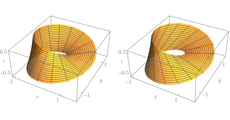
Figure 1. Two realizations of the Möbius strip: the common one (left panel) and the simple one (right panel), both with $\delta=3/5$.

The“moving segment” heuristics concerning the simple realization of the Möbius strip is confirmed and detailed in

Theorem 1.1.

The map $P_{\delta}\ni(t,r)\mapsto\mathbf{w}(t,r)\in\mathbf{w}(P_{\delta})$ is a homeomorphism iff $\delta\leqslant\sqrt{2}$.

For any point $p=(t,r)\in P_{\delta}$, we use $\mathbf{w}(p)$ and $\mathbf{w}(t,r)$ interchangeably.

The necessary proofs are deferred to Section 2.

Introduce the following notation:

(1.3) $$Q_{\delta}:=\big{\{}(p_{1},p_{2})\in P_{\delta}^{2}\colon\ p_{1}\neq p_{2},\ \mathbf{w}(p_{1})=\mathbf{w}(p_{2})\big{\}}$$

(1.4) $$I_{\delta}:=\{\mathbf{w}(p_{1})\colon\ \exists p_{2}\ \,(p_{1},p_{2})\in Q_{\delta}\},$$

(1.5) $$c_{\delta}:=1\wedge\frac{\delta\vee\sqrt{2}}{2},\quad s_{\delta}:=2c_{\delta}\sqrt{1-c_{\delta}^{2}}.$$

So, the set $Q_{\delta}$ is the set of all pairs of distinct points in $P_{\delta}$ that are glued together by the map $\mathbf{w}$, whereas $I_{\delta}$ is the image under $\mathbf{w}$ of the set of all points in $P_{\delta}$ that are glued (by the map $\mathbf{w}$) together with a different point in $P_{\delta}$. Thus, $I_{\delta}$ may be referred to as the self-intersection set of the image $\mathbf{w}(P_{\delta})$ of $P_{\delta}$ under the map $\mathbf{w}$.

The proof of Theorem 1.1 is mainly based on the following proposition, which provides a detailed description of self-intersection properties of the simple Möbius strip realization.

Proposition 1.2.

Take any points $p_{1}=(t_{1},r_{1})$ and $p_{2}=(t_{2},r_{2})$ in $[0,2\pi)\times{\mathbb{R}}$. Then $(p_{1},p_{2})\in Q_{\delta}$ iff for some $k\in\{0,1\}$ one has

(1.6) $$t_{2}=(2k+1)\pi-t_{1},\quad r_{1}=-2\cos\tfrac{t_{1}}{2},\quad r_{2}=(-1)^{k+1}2\sin\tfrac{t_{1}}{2},\quad s_{\delta}\leqslant|\sin t_{1}|<1.$$

Moreover,

(1.7) $$I_{\delta}=\{(-1,0,s)\colon s_{\delta}\leqslant|s|<1\}.$$

In view of the definitions in (1.5), we always have $s_{\delta}\leqslant 1$, and $s_{\delta}=1$ iff $\delta\leqslant\sqrt{2}$. So, by (1.7), for the self-intersection set $I_{\delta}$ we have this:

(1.8) $$I_{\delta}=\emptyset\iff\delta\leqslant\sqrt{2}.$$

One may also note at this point that, if $\delta\geqslant 2$, then $s_{\delta}=0$ and hence the self-intersection set $I_{\delta}$ in this case is the entire open interval between the points $(-1,0,-1)$ and $(-1,0,1)$ in ${\mathbb{R}}^{3}$.

Viewing the entire image $\mathbf{w}(P_{\delta})$ of the Möbius strip, it is a bit problematic to see how it looks like near the self-intersection set $I_{\delta}$, because that is covered by folds of the surface. For instance, see Figure 2, which is the version of Figure 1 with $\delta=1.97$ instead of $\delta=3/5$.

Figure 2. Two realizations of the Möbius strip: the common one (left panel) and the simple one (right panel), both with $\delta=1.97$.

Therefore, let us prepare appropriate parts of the surface for better viewing of the self-intersection set $I_{\delta}$ and its neighborhood. Toward that end, suppose that $\delta>\sqrt{2}$, for the self-intersection set $I_{\delta}$ to be nonempty. Next, let

$$h_{2}:=h_{2}(\delta):=\arcsin\tfrac{\delta\wedge 2}{2}\in\big{(}\tfrac{\pi}{4},\tfrac{\pi}{2}\big{]}\quad\text{and}\quad h_{3}:=h_{3}(\delta):=\pi-h_{2}\in\big{[}\tfrac{\pi}{2},\tfrac{3\pi}{4}\big{)}.$$

Consider then the following parts of the image $\mathbf{w}(P_{\delta})$ of the Möbius strip $P_{\delta}$ under map $\mathbf{w}$:

$$S_{1,\mathsf{bot}} :=\big{\{}\mathbf{w}(t_{1},r)\colon t_{1}\in[\tfrac{\pi}{2},2h_{2}],\,r\in[-2\cos\tfrac{\pi}{4},-2\cos h_{2}]\big{\}},$$

$$S_{1,\mathsf{top}} :=\big{\{}\mathbf{w}(t_{1},r)\colon t_{1}\in[2h_{3},\tfrac{3\pi}{2}],\,r\in[-2\cos h_{3},-2\cos\tfrac{3\pi}{4}]\big{\}},$$

$$S_{2,\mathsf{bot}} :=\big{\{}\mathbf{w}(t_{2},r)\colon t_{2}\in[\pi-2h_{2},\tfrac{\pi}{2}],\,r\in[-2\sin h_{2},-2\sin\tfrac{\pi}{4}]\big{\}},$$

$$S_{2,\mathsf{top}} :=\big{\{}\mathbf{w}(t_{2},r)\colon t_{2}\in[\tfrac{3\pi}{2},3\pi-2h_{3}),\,r\in[2\sin\tfrac{3\pi}{4},2\sin h_{3}]\big{\}}.$$

Concerning the ranges of $t_{1}$, $t_{2}$, and $r$ in the above display, note that

$$[\tfrac{\pi}{2},2h_{2}]\times[-2\cos\tfrac{\pi}{4},-2\cos h_{2}] \subset(0,\pi]\times[-\sqrt{2},0]\subset[0,2\pi)\times[-\delta,\delta]=P_{\delta},$$

$$[2h_{3},\tfrac{3\pi}{2}]\times[-2\cos h_{3},-2\cos\tfrac{3\pi}{4}] \subset[\pi,2\pi)\times[0,\sqrt{2}]\subset[0,2\pi)\times[-\delta,\delta]=P_{\delta},$$

$$[\pi-2h_{2},\tfrac{\pi}{2}]\times[-2\sin h_{2},-2\sin\tfrac{\pi}{4}] \subset[0,\pi)\times[-\delta,-\sqrt{2}]\subset[0,2\pi)\times[-\delta,\delta]=P_{\delta},$$

$$[\tfrac{3\pi}{2},3\pi-2h_{3})\times[2\sin\tfrac{3\pi}{4},2\sin h_{3}] \subset(\pi,2\pi)\times[\sqrt{2},\delta]\subset[0,2\pi)\times[-\delta,\delta]=P_{\delta}.$$

So, each of the surfaces $S_{1,\mathsf{bot}},S_{1,\mathsf{top}},S_{2,\mathsf{bot}},S_{2,\mathsf{top}}$ is indeed a part of the image $\mathbf{w}(P_{\delta})$ of the Möbius strip $P_{\delta}$ under map $\mathbf{w}$.

Now we are ready to illustrate Proposition 1.2, which is done in Figure 2.

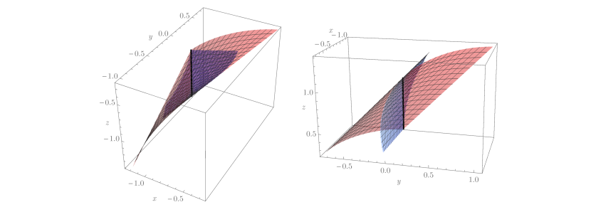
Figure 3. Parts of the image $\mathbf{w}(P_{\delta})$ of the Möbius strip $P_{\delta}$ under map $\mathbf{w}$ with $\delta=1.97$. Left panel: surfaces $S_{1,\mathsf{bot}}$ (red) and $S_{2,\mathsf{bot}}$ (blue), and the bottom half $\{(-1,0,s)\colon s_{\delta}\leqslant-s<1\}$ (thick, black) of the self-intersection set $I_{\delta}$. Right panel: surfaces $S_{1,\mathsf{top}}$ (red) and $S_{2,\mathsf{top}}$ (blue), and the top half $\{(-1,0,s)\colon s_{\delta}\leqslant s<1\}$ (thick, black) of the self-intersection set $I_{\delta}$. Here, $s(\delta)=s(1.97)\approx 0.34$.

In view of the above results and, in particular, Figure 2, it may seem unlikely that the simple Möbius strip realization is the closure of the graph of a rational function on a polynomially defined subset of ${\mathbb{R}}^{2}$. Yet, we have

Theorem 1.3.

For any real $\delta>0$, the image $\mathbf{w}(P_{\delta})$ of the Möbius strip $P_{\delta}$ under the map $\mathbf{w}$ coincides with the topological closure of the graph of a rational function $f\colon S_{\delta}\to{\mathbb{R}}$ on a polynomially defined set $S_{\delta}$, where

(1.9) $$f(x,y):=y-\frac{2(x+1)y}{(x+1)^{2}+y^{2}}=y\,\frac{x^{2}+y^{2}-1}{(x+1)^{2}+y^{2}}$$

for all $(x,y)\in S_{\delta}$,

(1.10) $$S_{\delta}:=\big{\{}(x,y)\in{\mathbb{R}}^{2}\setminus\{(-1,0)\}\colon g(x,y)\leqslant\delta^{2}\big{\}},\quad\text{and}\quad g(x,y):=\frac{(x^{2}+y^{2}-1)^{2}}{(x+1)^{2}+y^{2}}.$$

Clearly, the set $S_{\delta}$ is increasing in $\delta$, and $\bigcup_{\delta>0}S_{\delta}={\mathbb{R}}^{2}\setminus\{(-1,0)\}$. In Figure 4, one can see the sets $S_{\delta}$ with $\delta\in\{1/2,1,\sqrt{2},2,3\}$.

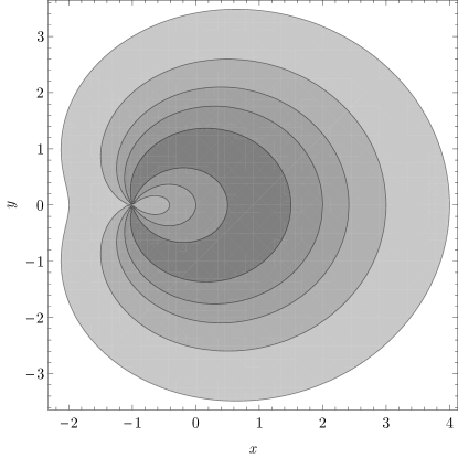
Figure 4. The increasing sets $S_{\delta}$ for $\delta\in\{\tfrac{1}{2},1,\sqrt{2},2,3\}$, from the darkest for $\delta=\tfrac{1}{2}$ to the lightest for $\delta=3$.

The proof of Theorem 1.3 is based on

Proposition 1.4.

One has

$$\mathbf{w}(P_{\delta})\setminus\ell=G(f),$$

where $\ell:=\{(-1,0,z)\colon z\in{\mathbb{R}}\}$ is the vertical line through point $(-1,0,0)$ in ${\mathbb{R}}^{3}$ and

(1.11) $$G(f):=\big{\{}\big{(}x,y,f(x,y)\big{)}\colon(x,y)\in S_{\delta}\big{\}}$$

is the graph of the function $f$.

Proposition 1.4 is complemented by

Proposition 1.5.

One has

(1.12) $$\mathbf{w}(P_{\delta})\cap\ell=J_{\delta}:=\{(-1,0,z)\colon|z|\leqslant\sigma_{\delta}\},$$

where

(1.13) $$\sigma_{\delta}:=2b_{\delta}\sqrt{1-b_{\delta}^{2}}\quad\text{and}\quad b_{\delta}:=\frac{\delta\wedge\sqrt{2}}{2}.$$

Clearly, it follows from (1.4) and (1.7) that $I_{\delta}\subseteq\mathbf{w}(P_{\delta})\cap\ell=J_{\delta}$. Here one may also note that $\sigma_{\delta}=1$ if $\delta\geqslant\sqrt{2}$.

Propositions 1.2 and 1.5 are illustrated in Figure 5.

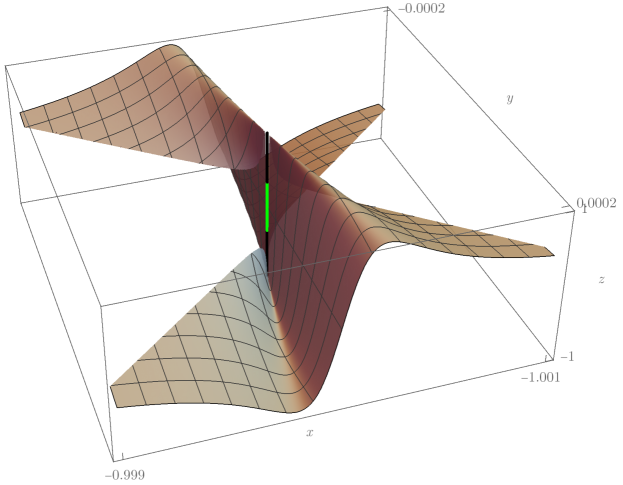
Figure 5. The part of the simple realization of the Möbius strip with $\delta=1.97$ in the neighborhood $[-1-\varepsilon,-1+\varepsilon]\times[-0.2\varepsilon,0.2\varepsilon]\times[-1-5\varepsilon,1+5\varepsilon]$ of the set $J_{\delta}$, with $\varepsilon=0.001$. Also shown are the sets $I_{\delta}$ (the union of the two black vertical segments) and $J_{\delta}\setminus I_{\delta}$ (the green vertical segment); here $s_{\delta}\approx 0.34$ and $\sigma_{\delta}=1$, so that $J_{\delta}$ is the entire vertical segment from point $(-1,0,-1)$ to point $(-1,0,1)$.

Immediately from Propositions 1.4 and 1.5, we obtain the following complete description of $\mathbf{w}(P_{\delta})$:

Corollary 1.6.

$\mathbf{w}(P_{\delta})=G(f)\cup\{(-1,0,z)\colon|z|\leqslant\sigma_{\delta}\}$.

Thus, the simple realization $\mathbf{w}(P_{\delta})$ of the Möbius strip is the union of a vertical segment with the graph of a rational function on a polynomially defined subset of ${\mathbb{R}}^{2}$. One should probably emphasize here that this conclusion holds for any, however large $\delta>0$. To state the following corollary, let us consider the infinite-width Möbius strip and its $\mathbf{w}$-image:

$$P_{\infty}:=\bigcup_{\delta>0}P_{\delta}=[0,2\pi)\times{\mathbb{R}}\quad\text{and}\quad\mathbf{w}(P_{\infty})=\bigcup_{\delta>0}\mathbf{w}(P_{\delta}).$$

For each $(x,y)\in{\mathbb{R}}^{2}$, consider also the corresponding vertical “cross-section” of the “entire” simple Möbius strip and its “cardinality”:

(1.14) $$Z_{\mathbf{w}}(x,y):=\{z\in{\mathbb{R}}\colon(x,y,z)\in\mathbf{w}(P_{\infty})\}\quad\text{and}\quad n_{\mathbf{w}}(x,y):=\operatorname{card}Z_{\mathbf{w}}(x,y),$$

where $\operatorname{card}S$ equals the cardinality of a set $S$ if $S$ is finite and equals $\infty$ otherwise. Then Corollary 1.6 immediately yields

Corollary 1.7.

$Z_{\mathbf{w}}(-1,0)=[-1,1]$ and $n_{\mathbf{w}}(x,y)=1$ for all $(x,y)\in{\mathbb{R}}^{2}\setminus\{(-1,0)\}$.

***

Whereas the common Möbius strip realization $\mathbf{v}(P_{\delta})$ looks similar to $\mathbf{w}(P_{\delta})$ for small enough half-width $\delta$, the situation changes dramatically when $\delta$ is large enough. It is known and straightforward to check that for each real $\delta>0$ the common Möbius strip realization $\mathbf{v}(P_{\delta})$ is a part of the cubic surface given by the “implicit” equation

$$-y+x^{2}y+y^{3}-2xz-2x^{2}z-2y^{2}z+yz^{2}=0;$$

see e.g. [1]. Since the left-hand side of this equation is a quadratic polynomial in $z$, one may expect that, in contrast with the simple realization $\mathbf{w}(P_{\delta})$ of the Möbius strip, the common realization $\mathbf{v}(P_{\delta})$ is “mainly” the union of the graphs of two algebraic (but not rational) functions. Proposition 1.8 below confirms and details such an expectation.

Define $Z_{\mathbf{v}}(x,y)$ and $n_{\mathbf{v}}(x,y)$ the same way $Z_{\mathbf{w}}(x,y)$ and $n_{\mathbf{w}}(x,y)$ were defined in (1.14), but using $\mathbf{v}$ instead of $\mathbf{w}$. We have the following counterpart of Corollary 1.7:

Proposition 1.8.

For any $(x,y)\in{\mathbb{R}}^{2}$,

(1.15) $$n_{\mathbf{v}}(x,y)=\left\{\begin{aligned} 2&\text{\quad if\quad}x\neq-1\ \&\ y\neq 0,\\ 1&\text{\quad if\quad}x=-1\ \&\ y\neq 0,\\ 1&\text{\quad if\quad}x\notin\{-1,0\}\ \&\ y=0,\\ \infty&\text{\quad if\quad}x\in\{-1,0\}\ \&\ y=0.\end{aligned}\right.$$

Moreover, $Z_{\mathbf{v}}(-1,0)=Z_{\mathbf{v}}(0,0)={\mathbb{R}}$.

So, the “typical” vertical “cross-section” of the “entire” common Möbius strip consists of precisely two points. Moreover, going over the lines of the proof of Proposition 1.8, one can see that the set of all points $(x,y)\in{\mathbb{R}}^{2}$ for which the vertical “cross-section” of the common Möbius strip $\mathbf{v}(P_{\delta})$ contains exactly two distinct points is of positive Lebesgue measure if $\delta>\sqrt{2}$ (but not if $\delta\leqslant\sqrt{2}$); in particular, look at (2.14) and note that

$$\inf_{\theta\in(0,\pi)}\Big{[}\Big{(}\dfrac{\rho-1}{\cos\tfrac{\theta}{2}}\Big{)}^{2}\,\vee\Big{(}\dfrac{\rho+1}{\sin\tfrac{\theta}{2}}\Big{)}^{2}\Big{]}=(\rho-1)^{2}+(\rho+1)^{2}=2+2\rho^{2},$$

which is greater than $2$ for any $\rho>0$, but is however close to $2$ if $\rho$ is small enough.

For the common Möbius strip realization, we have the following counterpart of Theorem 1.1:

Theorem 1.9.

The map $P_{\delta}\ni(t,r)\mapsto\mathbf{v}(t,r)\in\mathbf{v}(P_{\delta})$ is a homeomorphism iff $\delta<2$.

In [2, 3], the common Möbius strip realization is given with $\delta\leqslant 1$, which may be compared with Theorem 1.9.

Theorem 1.9 and Proposition 1.8 are illustrated in Figure 6.

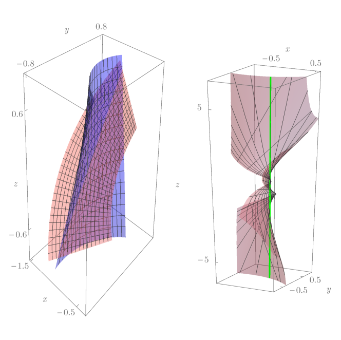
Figure 6. Parts of the image $\mathbf{v}(P_{\infty})$ of the Möbius strip $P_{\infty}$ under map $\mathbf{v}$. Left panel: Surfaces $\mathbf{v}\big{(}[0,\frac{\pi}{5}]\times[-2.5,-1.5]\big{)}$ (pink), $\mathbf{v}\big{(}[2\pi-\frac{\pi}{5},2\pi]\times[1.5,2.5]\big{)}$ (pink), and $\mathbf{v}\big{(}[\pi-\frac{\pi}{5},\pi+\frac{\pi}{5}]\times[-0.9,0.9]\big{)}$ (blue) – in a neighborhood of point $(-1,0,0)$. Right panel: Surface $\big{\{}\mathbf{v}\big{(}t,-\tfrac{1}{\cos(\tfrac{t}{2}+h)}\big{)}\colon t\in[0,2\pi],\,|h|\leqslant 0.5\big{\}}$ (pink) and a segment (green) of the vertical line $\ell$ through point $(0,0,0)$ – in a neighborhood of point $(0,0,0)$.

Significant efforts have been directed (see e.g. [4, 2, 5]) towards obtaining physically realizable – that is, requiring the least possible bending energy and no stretching/shrinking – models of the Möbius strip to be made from a paper band, in a sense culminating in [5]. However, the corresponding equations in those papers are much more complicated than (1.2) and even (1.1); only numerical solutions were given in [5] for the physically realizable model of a paper Möbius strip presented there.

2. Proofs

Modulo Proposition 1.2, the following is easy:

Proof of Theorem 1.1.

It is not hard to see that the Möbius strip $P_{\delta}$ is compact in its topology. Also, since $\mathbf{w}(2\pi-,r)=\mathbf{w}(0,-r)$ for $r\in[-\delta,\delta]$, it is easy to check that the map $\mathbf{w}$ is continuous. It follows that $\mathbf{w}$ is homeomorphic iff it is one-to-one. It remains to refer to (1.8). ∎

We still have to provide

Proof of Proposition 1.2.

Suppose that $(p_{1},p_{2})\in Q_{\delta}$, so that $(t_{1},r_{1})$ and $(t_{2},r_{2})$ are distinct points in $P_{\delta}$ such that $\mathbf{w}(t_{1},r_{1})=\mathbf{w}(t_{2},r_{2})$. Then, by (1.2), $\sin t_{1}+r_{1}\sin\tfrac{t_{1}}{2}=\sin t_{2}+r_{2}\sin\tfrac{t_{2}}{2}$ and $r_{1}\sin\tfrac{t_{1}}{2}=r_{2}\sin\tfrac{t_{2}}{2}$, whence $\sin t_{1}=\sin t_{2}$. Because the points $(t_{1},r_{1})$ and $(t_{2},r_{2})$ are in $P_{\delta}$ and hence $t_{1}$ and $t_{2}$ are in $[0,2\pi)$, it follows that either $t_{1}=t_{2}$ or $t_{1}+t_{2}=(2k+1)\pi$ for some $k\in\{0,1\}$.

If $t_{1}=t_{2}=:t$, then (1.2) implies $\cos t+r_{1}\cos\tfrac{t}{2}=\cos t+r_{2}\cos\tfrac{t}{2}$ and $r_{1}\sin\tfrac{t}{2}=r_{2}\sin\tfrac{t}{2}$. Since $\cos^{2}\tfrac{t}{2}+\sin^{2}\tfrac{t}{2}=1\neq 0$, we have $(t_{1},r_{1})=(t_{2},r_{2})$, which is a contradiction.

So, $t_{1}\neq t_{2}$ and $t_{1}+t_{2}=(2k+1)\pi$ for some $k\in\{0,1\}$, whence $t_{1}+t_{2}\in\{\pi,3\pi\}$. In particular, this verifies the first condition in (1.6). It also follows that

(2.1) $$\cos\tfrac{t_{2}}{2}=(-1)^{k}\sin\tfrac{t_{1}}{2}\quad\text{and}\quad\sin\tfrac{t_{2}}{2}=(-1)^{k}\cos\tfrac{t_{1}}{2}.$$

Therefore, the assumption $\mathbf{w}(t_{1},r_{1})=\mathbf{w}(t_{2},r_{2})$ implies the following system of linear equations:

(2.2) $$r_{1}\cos\tfrac{t_{1}}{2}+2\cos^{2}\tfrac{t_{1}}{2}=(-1)^{k}r_{2}\sin\tfrac{t_{1}}{2}+2\sin^{2}\tfrac{t_{1}}{2}\quad\text{and}\quad r_{1}\sin\tfrac{t_{1}}{2}=(-1)^{k}r_{2}\cos\tfrac{t_{1}}{2}$$

for $r_{1}$ and $r_{2}$. The determinant of this system is $(-1)^{k}(\sin^{2}\tfrac{t_{1}}{2}-\cos^{2}\tfrac{t_{1}}{2})=\break(-1)^{k+1}\cos t_{1}$. If it is zero, then $t_{1}\in\{\pi/2,3\pi/2\}$; hence, in view of the conditions $t_{1}+t_{2}\in\{\pi,3\pi\}$ and $t_{1}\in[0,2\pi)$ and $t_{2}\in[0,2\pi)$, we have either $t_{1}=\pi/2=t_{2}$ or $t_{1}=3\pi/2=t_{2}$, which contradicts the conclusion that $t_{1}\neq t_{2}$. So,

(2.3) $$t_{1}\notin\{\pi/2,3\pi/2\},$$

the determinant is nonzero, and hence the system (2.2) has a unique solution – which is given by the formula

(2.4) $$r_{1}=-2\cos\tfrac{t_{1}}{2}\quad\text{and}\quad r_{2}=(-1)^{k+1}2\sin\tfrac{t_{1}}{2},$$

for each $k\in\{0,1\}$. This verifies the second and third conditions in (1.6).

Moreover, because the points $(t_{1},r_{1})$ and $(t_{2},r_{2})$ are in $P_{\delta}$, we have $|r_{1}|\vee|r_{2}|\leqslant\delta$. That is, in view of (2.4), (2.3), and (1.5),

(2.5) $$t_{1}\in T_{\delta}:= \{t\in[0,2\pi)\colon\sqrt{2}<|2\cos\tfrac{t}{2}|\vee|2\sin\tfrac{t}{2}|\leqslant\delta\}$$

$$= \{t\in[0,2\pi)\colon s_{\delta}\leqslant|\sin t|<1\},$$

which completes the verification of all the four conditions in (1.6) – under the assumption that $(p_{1},p_{2})\in Q_{\delta}$.

Vice versa, assume now that the conditions in (1.6) hold for some points $p_{1}=(t_{1},r_{1})$ and $p_{2}=(t_{2},r_{2})$ in $[0,2\pi)\times{\mathbb{R}}$ and some $k\in\{0,1\}$, and let us then show that $(p_{1},p_{2})\in Q_{\delta}$. This is easy to do, as the above reasoning in this proof is essentially reversible. Anyway, recall here that the first condition in (1.6) implies (2.1). So, it follows from (1.2) and the first three conditions in (1.6) that

(2.6) $$\mathbf{w}(t_{1},r_{1})=\mathbf{w}(t_{2},r_{2})=(-1,0,-\sin t_{1}),$$

which verifies the last condition in the definition (1.3) of $Q_{\delta}$.

The last condition in (1.6) implies that $t_{1}\notin\{\pi/2,3\pi/2\}$. Hence, by the first condition in (1.6), $t_{1}\neq t_{2}$, which verifies the condition $p_{1}\neq p_{2}$ in the definition (1.3) of $Q_{\delta}$.

The last three conditions in (1.6) together with the second line in (2.5) imply that $|r_{1}|\vee|r_{2}|\leqslant\delta$, which verifies the condition $(p_{1},p_{2})\in P_{\delta}^{2}$ in the definition (1.3) of $Q_{\delta}$. Thus, the first part of Proposition 1.2 is proved.

It remains to prove (1.7). Take any $(x,y,z)\in I_{\delta}$. Then, by (1.4), there exists some $(p_{1},p_{2})\in Q_{\delta}$ such that $\mathbf{w}(p_{1})=(x,y,z)$. So, by the just proved first part of Proposition 1.2, for some points $p_{1}=(t_{1},r_{1})$ and $p_{2}=(t_{2},r_{2})$ in $[0,2\pi)\times{\mathbb{R}}$ the conditions in (1.6) hold. So, in view of (2.6), $(x,y,z)=(-1,0,s)$ for $s:=-\sin t_{1}$, and then also $s_{\delta}\leqslant|s|<1$, so that $(x,y,z)$ belongs to the set on the right-hand side of equality (1.7).

Vice versa, take any $s$ such that $s_{\delta}\leqslant|s|<1$. To complete the proof of Proposition 1.2, it now remains to show that $(-1,0,s)\in I_{\delta}$. Clearly, the condition $s_{\delta}\leqslant|s|<1$ implies that there is some $t\in(0,2\pi)$ such that $s=-\sin t_{1}$, so that the last condition in (1.6) is satisfied. Next, there is some $k\in\{0,1\}$ such that $k\pi<t_{1}\leqslant(k+1)\pi$. Further, take $t_{2}$, $r_{1}$, and $r_{2}$ according to the first three conditions in (1.6). Then $0\leqslant t_{2}<2\pi$ and, by the first part of Proposition 1.2, for the resulting points $p_{1}=(t_{1},r_{1})$ and $p_{2}=(t_{2},r_{2})$ one has $(p_{1},p_{2})\in Q_{\delta}$. Moreover, again by (2.6), indeed $(-1,0,s)=(-1,0,-\sin t_{1})\in I_{\delta}$.

Proposition 1.2 is now completely proved. ∎

Assuming that Proposition 1.4 holds, it is easy to complete

Proof of Theorem 1.3.

The image $\mathbf{w}(P_{\delta})$ of the compact set $P_{\delta}$ under the continuous map $\mathbf{w}$ is compact and hence closed. So, in view of Proposition 1.4, it suffices to show that the set $\mathbf{w}(P_{\delta})\setminus\ell$ is dense in $\mathbf{w}(P_{\delta})$.

To do this, take any $(t,r)\in P_{\delta}$ such that $\mathbf{w}(t,r)\in\ell$, so that $\mathbf{w}(t,r)=(-1,0,z)$ for some $z\in{\mathbb{R}}$. We only need to show that this point, $\mathbf{w}(t,r)=(-1,0,z)$, can be approximated however closely by points in $\mathbf{w}(P_{\delta})\setminus\ell$.

Consider first the case $r=0$. Then, by (1.2), the condition $\mathbf{w}(t,r)=(-1,0,z)$ implies that $\cos t=-1$ and hence $t=\pi$ and $\mathbf{w}(t,r)=(-1,0,0)$. Take now any $\varepsilon\in(0,\pi)$. Then $(\pi+\varepsilon,0)\in P_{\delta}$ and $\mathbf{w}(\pi+\varepsilon,0)=(-\cos\varepsilon,-\sin\varepsilon,0)\in\mathbf{w}(P_{\delta})\setminus\ell$. Moreover, letting $\varepsilon\downarrow 0$, we have $\mathbf{w}(\pi+\varepsilon,0)\to(-1,0,0)=\mathbf{w}(t,r)$, thus obtaining the desired approximation.

Assume now that $r\neq 0$. Then for any $\varepsilon\in(0,1)$ one has $(t,(1-\varepsilon)r)\in P_{\delta}$ and $\mathbf{w}(t,(1-\varepsilon)r)=(-1-r\varepsilon\cos\frac{t}{2},-r\varepsilon\sin\frac{t}{2},z-r\varepsilon\sin\frac{t}{2})\in\mathbf{w}(P_{\delta})\setminus\ell$. Moreover, letting $\varepsilon\downarrow 0$, we have $\mathbf{w}(t,(1-\varepsilon)r)\to(-1,0,z)=\mathbf{w}(t,r)$, thus obtaining the desired approximation in the latter case as well. ∎

We still have to provide

Proof of Proposition 1.4.

Let us first show that $\mathbf{w}(P_{\delta})\setminus\ell\subseteq G(f)$. To do that, take any $(x,y,z)\in\mathbf{w}(P_{\delta})\setminus\ell$, so that $(x,y)\neq(-1,0)$ and (1.2) holds for some $(t,r)\in P_{\delta}=[0,2\pi)\times[-\delta,\delta]$. We want then to show that $(x,y)\in S_{\delta}$ and $f(x,y)=z$.

By (1.2),

(2.7) $$x\sin\tfrac{t}{2}-y\cos\tfrac{t}{2}=\cos t\sin\tfrac{t}{2}-\sin t\cos\tfrac{t}{2}=-\sin\tfrac{t}{2}.$$

Also, the condition $(t,r)\in P_{\delta}$ implies that $0\leqslant\tfrac{t}{2}<\pi$. So, if $\sin\tfrac{t}{2}=0$, then $t=0$ and hence, by (1.2), (1.9), and (1.10), $(x,y,z)=\mathbf{w}(t,r)=(1+r,0,0)$, $f(x,y)=0=z$, and $g(x,y)=r^{2}\leqslant\delta^{2}$. Thus, $(x,y)\in S_{\delta}$ and $f(x,y)=z$ – in the case when $\sin\tfrac{t}{2}=0$.

Consider now the case when $\sin\tfrac{t}{2}\neq 0$. Then (2.7) yields $x+1=y\cot\tfrac{t}{2}$. So, $y=0$ would imply $x=-1$, in contradiction with the condition $(x,y)\neq(-1,0)$. It follows that $y\neq 0$. Since $0\leqslant\tfrac{t}{2}<\pi$, we have

(2.8) $$\cot\tfrac{t}{2}=\tfrac{x+1}{y},\quad t=2\operatorname{arccot}\tfrac{x+1}{y},\quad\sin t=\frac{2y(x+1)}{(x+1)^{2}+y^{2}};$$

here we use the convention that the values of the function $\operatorname{arccot}$ are in the interval $(0,\pi)$. Now, by (1.2) and (1.9),

(2.9) $$z=y-\sin t=y-\frac{2y(x+1)}{(x+1)^{2}+y^{2}}=f(x,y).$$

Moreover, the conditions $(t,r)\in P_{\delta}$, (1.2), $\sin\tfrac{t}{2}\neq 0$, (2.8), (2.9), (1.9), and (1.10) yield

$$\delta^{2}\geqslant r^{2}=\frac{z^{2}}{\sin^{2}\tfrac{t}{2}}=z^{2}(1+\cot^{2}\tfrac{t}{2})=z^{2}\,\frac{(x+1)^{2}+y^{2}}{y^{2}}=f(x,y)^{2}\,\frac{(x+1)^{2}+y^{2}}{y^{2}}\\ =g(x,y),$$

so that $(x,y)\in S_{\delta}$. Thus, in the case $\sin\tfrac{t}{2}\neq 0$ as well, we have $(x,y)\in S_{\delta}$ and $f(x,y)=z$. This proves that $\mathbf{w}(P_{\delta})\setminus\ell\subseteq G(f)$.

It remains to prove that $G(f)\subseteq\mathbf{w}(P_{\delta})\setminus\ell$. To do this, take any $(x,y,z)\in G(f)$, so that $(x,y)\in S_{\delta}$ and $f(x,y)=z$. In view of (1.11) and (1.10), $G(f)\cap\ell=\emptyset$. So, it suffices to show that (1.2) holds for some $(t,r)\in P_{\delta}=[0,2\pi)\times[-\delta,\delta]$.

If $y=0$, then $z=f(x,0)=0$, and the condition $(x,y)\in S_{\delta}$ implies $(x-1)^{2}=g(x,y)\leqslant\delta^{2}$ and (1.2) obviously holds for $(t,r)=(0,x-1)\in P_{\delta}=[0,2\pi)\times[-\delta,\delta]$.

Consider now the case $y\neq 0$. Let then

$$t:=2\operatorname{arccot}\frac{x+1}{y}\quad\text{and}\quad r:=\frac{y-\sin t}{\sin\frac{t}{2}}=\frac{y}{\sin\frac{t}{2}}-2\cos\tfrac{t}{2},$$

whence

$$t\in(0,2\pi),\quad\sin\tfrac{t}{2}=\frac{|y|}{\sqrt{(x+1)^{2}+y^{2}}}>0,\quad\cos\tfrac{t}{2}=\frac{(x+1)\operatorname{sign}y}{\sqrt{(x+1)^{2}+y^{2}}},$$

$$\sin t=\frac{2(x+1)y}{(x+1)^{2}+y^{2}},\quad\cos t=\frac{(x+1)^{2}-y^{2}}{(x+1)^{2}+y^{2}},$$

$$\quad\cos t+r\cos\tfrac{t}{2}=x,\quad\sin t+r\sin\tfrac{t}{2}=y,\quad r^{2}=g(x,y)^{2}\leqslant\delta^{2}.$$

So, $(t,r)\in P_{\delta}$. Moreover, it follows from (1.2), the last line of the above display, the condition $y\neq 0$, and the already proved set inclusion $\mathbf{w}(P_{\delta})\setminus\ell\subseteq G(f)$ that for some $\tilde{z}\in{\mathbb{R}}$ one has $(x,y,\tilde{z})=\mathbf{w}(t,r)\in\mathbf{w}(P_{\delta})\setminus\ell\subseteq G(f)$. But it was assumed that $(x,y,z)\in G(f)$, and $f$ is a function. We conclude that $\tilde{z}=z$, whence $\mathbf{w}(t,r)=(x,y,z)$; that is, indeed (1.2) holds for the point $(t,r)\in P_{\delta}$ constructed above. ∎

Proof of Proposition 1.5.

Let us first show that $\mathbf{w}(P_{\delta})\cap\ell\subseteq J_{\delta}$. Take any $(x,y,z)\in\mathbf{w}(P_{\delta})\cap\ell$, so that $x=-1$, $y=0$, and (1.2) holds for some $(t,r)\in P_{\delta}$. Hence, $t\in[0,2\pi)$, $|r|\leqslant\delta$, $-1=x=\cos t+r\cos\tfrac{t}{2}$, $0=y=\sin t+r\sin\tfrac{t}{2}$, and $z=r\sin\tfrac{t}{2}$.

If $\sin\tfrac{t}{2}=0$, then $z=0$ and hence $(x,y,z)\in J_{\delta}$.

Suppose now that $\sin\tfrac{t}{2}\neq 0$. Then $0=y=\sin t+r\sin\tfrac{t}{2}$ yields $r=-2\cos\tfrac{t}{2}$ and hence $\delta\geqslant|r|=2|\cos\tfrac{t}{2}|$ and $z=r\sin\tfrac{t}{2}=-\sin t$. On the other hand,

(2.10) $$\big{\{}-\sin t\colon t\in[0,2\pi),\,2|\cos\tfrac{t}{2}|\leqslant\delta\big{\}}=[-\sigma_{\delta},\sigma_{\delta}].$$

So, $(x,y,z)\in J_{\delta}$ in the case $\sin\tfrac{t}{2}\neq 0$ as well, which verifies the set inclusion $\mathbf{w}(P_{\delta})\cap\ell\subseteq J_{\delta}$.

The above reasoning is essentially reversible. Indeed, take any $(x,y,z)\in J_{\delta}$, so that $x=-1$, $y=0$, and $z\in[-\sigma_{\delta},\sigma_{\delta}]$. By (2.10), we can find some $t\in[0,2\pi)$ such that $z=-\sin t$ and $2|\cos\tfrac{t}{2}|\leqslant\delta$. Letting now $r:=-2\cos\tfrac{t}{2}$, we have $|r|\leqslant\delta$, so that $(t,r)\in P_{\delta}$; moreover, then $(x,y,z)=(-1,0,-\sin t)=\mathbf{w}(t,r)$ by (1.2), so that $(x,y,z)\in w(P_{\delta})\cap\ell$. This verifies the set inclusion $J_{\delta}\subseteq\mathbf{w}(P_{\delta})\cap\ell$ and thus completes the proof of Proposition 1.5. ∎

Proof of Proposition 1.8.

Take any $(x,y)\in{\mathbb{R}}^{2}$. Let

$$P(x,y) :=\big{\{}(t,r)\in P_{\infty}\colon(1+r\cos\tfrac{t}{2})\cos t=x,\,(1+r\cos\tfrac{t}{2})\sin t=y\big{\}},$$

$$N(x,y) :=\operatorname{card}P(x,y).$$

In view of (1.1),

$$Z_{\mathbf{v}}(x,y)=\big{\{}r\sin\tfrac{t}{2}\colon(t,r)\in P(x,y)\big{\}},$$

whence

(2.11) $$n_{\mathbf{v}}(x,y)=\operatorname{card}Z_{\mathbf{v}}(x,y)\leqslant\operatorname{card}P(x,y)=N(x,y).$$

Consider also the pair $(\rho,\theta)=\big{(}\rho(x,y),\theta(x,y)\big{)}$ of the “polar coordinates” of the point $(x,y)$, which is uniquely determined by the conditions

(2.12) $$(x,y)=\rho(\cos\theta,\sin\theta)\quad\text{and}\quad(\rho,\theta)\in{\mathbb{R}}\times[0,\pi),$$

provided that $(x,y)\neq(0,0)$. The choice $[0,\pi)$ for the range of values of $\theta$ will be convenient, because it implies that

(2.13) $$\cos\tfrac{\theta}{2}\neq 0.$$

Proposition 1.8 will easily follow from a few lemmas:

Lemma 2.1.

$Z_{\mathbf{v}}(0,0)={\mathbb{R}}$.

Proof of Lemma 2.1.

Take any $z\in{\mathbb{R}}$ and let $t:=-2\arctan z+2\pi\mathrm{I}\!\left\{z>0\right\}$, where $\mathrm{I}\!\left\{\cdot\right\}$ denotes the indicator function. Then $t\in[0,2\pi)\setminus\{\pi\}$, so that $\cos\tfrac{t}{2}\neq 0$. Let now $r:=-1/\cos\tfrac{t}{2}$. Then $\mathbf{v}(t,r)=(0,0,z)$. It remains to recall the definition of $Z_{\mathbf{v}}$ (cf. (1.14)). ∎

Lemma 2.2.

$Z_{\mathbf{v}}(-1,0)={\mathbb{R}}$.

Proof of Lemma 2.2.

For all $z\in{\mathbb{R}}$ one has $\mathbf{v}(\pi,z)=(-1,0,z)$. ∎

Lemma 2.3.

$n_{\mathbf{v}}(x,y)\geqslant 1$.

Proof of Lemma 2.3.

Let $r:=(\rho-1)/\cos\tfrac{\theta}{2}$; this definition makes sense, in view of (2.13). Then, by (1.1), $\mathbf{v}(\theta,r)=(x,y,z)$ for some $z\in{\mathbb{R}}$. Hence, $Z_{\mathbf{v}}(x,y)\neq\emptyset$ and $n_{\mathbf{v}}(x,y)\geqslant 1$. ∎

Lemma 2.4.

Suppose that $x\notin\{-1,0\}$ and $y=0$. Then $n_{\mathbf{v}}(x,y)=1$.

Proof of Lemma 2.4.

Take any $(t,r)\in P(x,0)$, so that $(1+r\cos\tfrac{t}{2})\cos t=x\neq 0$ and $(1+r\cos\tfrac{t}{2})\sin t=0$. Then $1+r\cos\tfrac{t}{2}\neq 0$, $\sin t=0$, and $t\in\{0,\pi\}$. If $t=\pi$, then $x=-1$, a contradiction. So, $t=0$, $1+r=x$, and $r=x-1$. This means that $P(x,0)\subseteq\{(0,x-1)\}$ and $N(x,0)\leqslant 1$. It remains to recall that $n_{\mathbf{v}}(x,y)\leqslant N(x,y)$ (by (2.11)) and refer to Lemma 2.3. ∎

Lemma 2.5.

Suppose that $y\neq 0$. Then $n_{\mathbf{v}}(x,y)=1$ if $x=-1$ and $n_{\mathbf{v}}(x,y)=2$ if $x\neq-1$.

Proof of Lemma 2.5.

In view of (1.1) and the condition $y\neq 0$, for any $(t,r)\in P(x,y)$ one has $\sin t\neq 0$ and hence $\cos\tfrac{t}{2}\neq 0$, so that $r$ is uniquely determined, by the formula $r=\big{(}\tfrac{y}{\sin t}-1\big{)}/\cos\tfrac{t}{2}$, given $t$ and the condition $(t,r)\in P(x,y)$. Therefore, by (2.12), the condition that two points in $P(x,y)$ are distinct means precisely that they are of the form $(\theta,r_{1})$ and $(\theta+\pi,r_{2})$ for some $\theta\in[0,\pi)$ and real $r_{1}$ and $r_{2}$ such that $1+r_{1}\cos\tfrac{\theta}{2}=\rho=-(1+r_{2}\cos\tfrac{\theta+\pi}{2})$ or, equivalently,

(2.14) $$r_{1}=\dfrac{\rho-1}{\cos\tfrac{\theta}{2}}\quad\text{and}\quad r_{2}=\dfrac{\rho+1}{\sin\tfrac{\theta}{2}}.$$

Here we have taken into account that $\cos\tfrac{\theta}{2}\neq 0$ (because $\theta\in[0,\pi)$) and $\sin\tfrac{\theta}{2}\neq 0$ (because otherwise $\theta=0$ and hence $y=\rho\sin\theta=0$). So, here $P(x,y)=\Big{\{}\Big{(}\theta,\dfrac{\rho-1}{\cos\tfrac{\theta}{2}}\Big{)},\Big{(}\theta+\pi,\dfrac{\rho+1}{\sin\tfrac{\theta}{2}}\Big{)}\Big{\}}$. Hence, in view of (1.1) and (2.14), the condition $n_{\mathbf{v}}(x,y)=1$ means precisely that $\dfrac{\rho-1}{\cos\tfrac{\theta}{2}}\,\sin\tfrac{\theta}{2}=\dfrac{\rho+1}{\sin\tfrac{\theta}{2}}\,\sin\tfrac{\theta+\pi}{2}$, which can be rewritten as $\rho\cos\theta=-1$ or simply as $x=-1$. It also follows that in the remaining case when $x\neq-1$ one has $n_{\mathbf{v}}(x,y)=2$. ∎

Now the first two lines in (1.15) follow by Lemma 2.5, the third line there by Lemma 2.4. *, and the fourth line there by Lemmas 2.2 and 2.2. The second sentence in Proposition 1.8 and hence the fourth line in (1.15) follow by Lemmas 2.2 and 2.2.

Proposition 1.8 is thus completely proved. ∎

Proof of Theorem 1.9.

As in the proof of Theorem 1.1, here it is easy to see that the map $P_{\delta}\ni(t,r)\mapsto\mathbf{v}(t,r)\in\mathbf{v}(P_{\delta})$ is a homeomorphism iff it is one-to-one.

Next, suppose that $\delta\geqslant 2$. Then $(0,-2)$ and $(\pi,0)$ are distinct points in $P_{\delta}$ and, in view of (1.1), $\mathbf{v}(0,-2)=(-1,0,0)=\mathbf{v}(\pi,0)$. So, the map $P_{\delta}\ni(t,r)\mapsto\mathbf{v}(t,r)\in\mathbf{v}(P_{\delta})$ is not one-to-one if $\delta\geqslant 2$.

Suppose now that $\delta<2$. Take any points $(t_{1},r_{1})$ and $(t_{2},r_{2})$ such that $\mathbf{v}(t_{1},r_{1})=\mathbf{v}(t_{2},r_{2})=:(x,y,z)$. We have then to show that $(t_{1},r_{1})=(t_{2},r_{2})$.

If $t_{1}=t_{2}=:t$, then, by (1.1),

(2.15) $$0=\|\mathbf{v}(t,r_{1})-\mathbf{v}(t,r_{2})\|^{2}=(r_{1}-r_{2})^{2},$$

where $\|\cdot\|$ denotes the Euclidean norm on ${\mathbb{R}}^{3}$. Hence, $r_{1}=r_{2}$, and the desired conclusion $(t_{1},r_{1})=(t_{2},r_{2})$ follows, whenever $t_{1}=t_{2}$. So, w.l.o.g. $t_{1}\neq t_{2}$.

Next, consider the case when $\cos t_{1}=0=\cos t_{2}$, so that w.l.o.g. $t_{1}=\tfrac{\pi}{2}$ and $t_{2}=\tfrac{3\pi}{2}$, whence, in view of (1.1), $[y=]1+r_{1}/\sqrt{2}=-1+r_{2}/\sqrt{2}$ and $[z=]r_{1}/\sqrt{2}=r_{2}/\sqrt{2}$, so that $r_{1}=r_{2}=:r$ and $1+r/\sqrt{2}=-1+r/\sqrt{2}$, which is a contradiction. Hence, the case when $\cos t_{1}=0=\cos t_{2}$ is impossible, given the other conditions.

Further, consider the case when exactly one of the numbers $\cos t_{1}$ and $\cos t_{2}$ is $0$. Then w.l.o.g. $\cos t_{1}=0\neq\cos t_{2}$, which implies $t_{1}=\pi+\varepsilon\tfrac{\pi}{2}$ for some $\varepsilon\in\{-1,1\}$, $x=0$, $1+r_{2}\cos\tfrac{t_{2}}{2}=0$, $y=0$, $1-r_{1}\varepsilon/\sqrt{2}=1+r_{1}\cos\tfrac{t_{1}}{2}=\varepsilon y=0$, $r_{1}=\varepsilon\sqrt{2}$, and $z=r_{1}\sin\tfrac{t_{1}}{2}=\varepsilon=r_{2}\sin\tfrac{t_{2}}{2}$. Further, equalities $1+r_{2}\cos\tfrac{t_{2}}{2}=0$ and $\varepsilon=r_{2}\sin\tfrac{t_{2}}{2}$ yield $\tan\tfrac{t_{2}}{2}=-\varepsilon$, whence $\cos t_{2}=0$, which contradicts the current case condition.

Further yet, consider the case when $\cos t_{1}\neq 0$ and $\cos t_{2}\neq 0$ but $x=0$. Then $1+r_{1}\cos\tfrac{t_{1}}{2}=0=1+r_{2}\cos\tfrac{t_{2}}{2}$ and $r_{1}\sin\tfrac{t_{1}}{2}=[z=]r_{2}\sin\tfrac{t_{2}}{2}$, whence $r_{1}=-1/\cos\tfrac{t_{1}}{2}$, $r_{2}=-1/\cos\tfrac{t_{2}}{2}$, $\tan\tfrac{t_{1}}{2}=\tan\tfrac{t_{2}}{2}$, and $t_{1}=t_{2}$, which contradicts the assumption $t_{1}\neq t_{2}$.

It remains to consider the case when $x\neq 0$, so that $\cos t_{1}\neq 0$ and $\cos t_{2}\neq 0$. Then, by (1.1), $\tan t_{1}=\tfrac{y}{x}=\tan t_{2}$, so that $|t_{1}-t_{2}|=\pi$. So, w.l.o.g. $t_{1}=t$ and $t_{2}=t+\pi$ for some $t\in[0,\pi)$. Hence, $[x=](1+r_{1}\cos\tfrac{t}{2})\cos t=(1-r_{2}\sin\tfrac{t}{2})(-\cos t)$ and $[y=](1+r_{1}\cos\tfrac{t}{2})\sin t=(1-r_{2}\sin\tfrac{t}{2})(-\sin t)$. Since $\cos t$ and $\sin t$ do not vanish simultaneously, we have $1+r_{1}\cos\tfrac{t}{2}=-(1-r_{2}\sin\tfrac{t}{2})$. Also, $r_{1}\sin\tfrac{t}{2}=[z=]r_{2}\cos\tfrac{t}{2}$. So, we have the system $r_{1}\cos\tfrac{t}{2}-r_{2}\sin\tfrac{t}{2}=-2$ and $r_{1}\sin\tfrac{t}{2}-r_{2}\cos\tfrac{t}{2}=0$ of linear equations for $r_{1},r_{2}$. Its determinant is $-\cos^{2}\tfrac{t}{2}+\sin^{2}\tfrac{t}{2}=-\cos t\neq 0$, and its only solution is given by $r_{1}=-2\cos\tfrac{t}{2}/\cos t$ and $r_{2}=-2\sin\tfrac{t}{2}/\cos t$, whence $\delta^{2}\geqslant r_{1}^{2}\vee r_{2}^{2}\geqslant|r_{1}^{2}-r_{2}^{2}|=4/|\cos t|\geqslant 4$, so that $\delta\geqslant 2$, which contradicts the assumption $\delta<2$.

This completes the proof of Theorem 1.9. ∎

References

- [1] E. W. Weisstein, Möbius strip. From MathWorld – A Wolfram Web Resource, http://mathworld.wolfram.com/MoebiusStrip.html (2016).
-
[2]
G. E. Schwarz, The dark side of the
Moebius strip, Amer. Math. Monthly 97 (10) (1990) 890–897.
URL http://dx.doi.org/10.2307/2324325 - [3] Wikipedia, Möbius strip, https://en.wikipedia.org/wiki/M%C3%B6bius_strip (2016).
- [4] B. Halpern, C. Weaver, Inverting a cylinder through isometric immersions and isometric embeddings, Trans. Amer. Math. Soc. 230 (1977) 41–70.
- [5] E. L. Starostin, G. H. M. van der Heijden, The shape of a Möbius strip, Nature Materials 6 (2007) 563–567.