∎
22email: sk2011@math.rutgers.edu 33institutetext: J.D. Mireles James 44institutetext: Florida Atlantic University, Department of Mathematical Sciences
44email: jmirelesjames@fau.edu
Homoclinic dynamics in a restricted four body problem ††thanks: The second author was partially supported by NSF grant DMS-1813501. Both authors were partially supported by NSF grant DMS-1700154 and by the Alfred P. Sloan Foundation grant G-2016-7320
Abstract
We describe a method for computing an atlas for the stable or unstable manifold attached to an equilibrium point, and implement the method for the saddle-focus libration points of the planar equilateral restricted four body problem. We employ the method at the maximally symmetric case of equal masses, where we compute atlases for both the stable and unstable manifolds. The resulting atlases are comprised of thousands of individual chart maps, with each chart represented by a two variable Taylor polynomial. Post-processing the atlas data yields approximate intersections of the invariant manifolds, which we refine via a shooting method for an appropriate two point boundary value problem. Finally, we apply numerical continuation to some of the BVP problems. This breaks the symmetries and leads to connecting orbits for some non-equal values of the primary masses.
Keywords:
Gravitational - body problem invariant manifolds high-order Taylor methods automatic differentiation numerical continuationpacs:
45.50.Jf 45.50.Pk 45.10.-b 02.60.Lj 05.45.AcMSC:
70K44 34C45 70F151 Introduction
Illuminating studies by Darwin, Strömgren, and Moulton in the first decades of the Twentieth Century established the importance of numerical calculations in the qualitative theory of Hamiltonian systems MR1554890 ; stromgrenRef ; moultonBook . In particular their work gave new insights into the orbit structure of the circular restricted three body problem (CRTBP), a problem already immortalized by Poincaré. Interest in the CRTBP was reinvigorated in the 1960’s with the inauguration of the space race and a number of authors including Szebehely, Nacozy, and Flandern szebehelyOnStromgren ; szebehelyTriangularPoints harnessed the newly available power of digital computing to settle some questions raised by Strömgren. The interested reader will find a delightful retelling of this story with many additional references in the book of Szebhely theoryOfOrbits .
Motivated by the works just mentioned, in 1973 Henrard proved a theorem settling a conjecture of Strömgren about the role of asymptotic orbits. More precisely, Henrard showed that the existence of a transverse homoclinic for a saddle-focus equilibrium in a two degrees of freedom Hamiltonian system implies the existence of a tube of periodic orbits parameterized by energy and accumulating to the homoclinic MR0365628 . In the same paper he showed that the period of the orbits in the family goes to infinity and their stability changes infinitely often as they accumulate to the homoclinic. This phenomena was called the blue sky catastrophe by Abraham MR813508 and has been studied by a number of authors including L.P. Shilnikov, A.L. Shilnikov, and Turaev MR3253906 , Devaney MR0431274 .
In 1976 it was further shown by Devaney that such a transverse homoclinic – again for a saddle-focus in a two degrees of freedom Hamiltonian system – implies the existence of chaotic dynamics in the energy level of the equilibrium MR0442990 . See also the works of Lerman MR998368 ; MR1135905 . Such theorems should be thought of as Hamiltonian versions of the homoclinic bifurcations studied by Shilńikov MR0259275 ; 0025-5734-10-1-A07 ; MR0210987 . Taken together the results cited so far paint a vivid picture of the rich dynamics near a transverse homoclinic connection in a two degree of freedom Hamiltonian system.
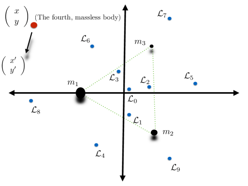
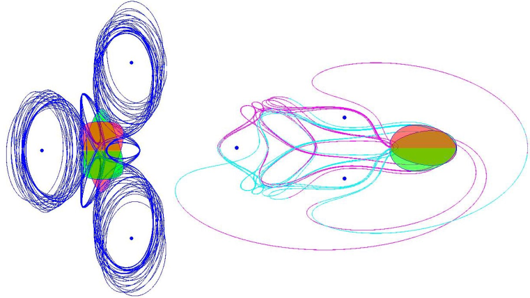
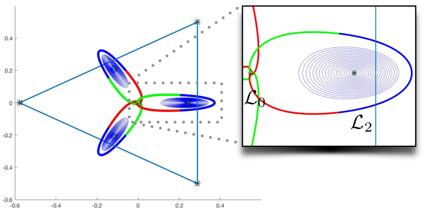
The present study concerns asymptotic orbits in the planar equilateral restricted four body problem, henceforth referred to as the circular restricted four body problem (CRFBP). The problem has a rich literature dating at least back to the work of Pedersen pedersen1 ; pedersen2 . Detailed numerical studies of the equilibrium set, as well as the planar and spatial Hill’s regions are found in Simó MR510556 , in Baltagiannis and Papadakis MR2845212 , and in Álvarez-Ramíerz and Vidal MR2596303 . Mathematically rigorous theorems about the equilibrium set and its bifurcations are proven by Leandro and Barros in MR2232439 ; MR2784870 ; MR3176322 (with computer assistance). They show that for any value of the masses there are either 8, 9, or 10 equilibrium solutions with 6 outside the equilateral triangle formed by the primary bodies (see Figure 1).
Fundamental families of periodic orbits are considered by Papadakis in MR3571218 ; MR3500916 , and by Burgos-García, Bengochea, and Delgado in burgosTwoEqualMasses ; MR3715396 . A study by Burgos-García, Lessard, and Mireles James proves the existence of some spatial periodic orbits for the CRFBP jpJaimeAndMe (again with computer assistance). An associated Hill’s problem is derived and its periodic orbits are studied by Burgos-García and Gidea in MR3554377 ; MR3346723 .
Regularization of collisions are studied by Álvarez-Ramírez, Delgado, and Vidal in MR3239345 . Chaotic motions were studied numerically by Gidea and Burgos in MR2013214 , and by Álvarez-Ramírez and Barrabés in MR3304062 . Perturbative proofs of the existence of chaotic motions are found in the work of She, Cheng and Li MR3626383 ; MR3158025 ; MR3038224 , and also in the work of Alvarez-Ramírez, García, Palacián, and Yanguas chaosCRFBP . Blue sky catastrophes in the CRFBP were previously studied by Burgos-García and Delgado in MR3105958 , and by Kepley and Mireles James in shaneAndJay . This last reference develops (computer assisted) methods of proof for verifying the hypotheses of the theorems of Hernard and Devaney.
The main goal of the present work is to study orbits which are homoclinic to a saddle-focus equilibrium solution in the equilateral restricted four body problem. We apply the parameterization method of Cabré, Fontich, and de la Llave to compute a chart for the stable or unstable manifold in a neighborhood of the equilibrium MR1976079 ; MR1976080 ; MR2177465 . Then, we implement the analytic continuation scheme for local invariant manifolds developed by Kalies, Kepley, and Mireles James in manifoldPaper1 , where it was applied to some two dimensional manifolds in the Lorenz system. We adapt this scheme for the CRFBP, and compute atlases for the local stable/unstable manifolds attached to a saddle-focus equilibrium. By an atlas we mean a collection of analytic maps or charts of the form, , where the image of lies in the stable or unstable manifold. The union of these charts is a piecewise approximation for a large portion of the manifold away from the equilibrium. For a more formal definition see any standard text on differential geometry. The charts are computed using high order polynomial approximations with algorithms that exploit automatic manipulations of formal series.
After computing the stable/unstable manifold atlases we post-process to find approximate intersections. Once a potential intersection is located we refine the approximation using a Newton scheme for a two point boundary value problem as in the classical work of Doedel, Friedman, and Kunin MR1007358 ; MR1456497 . In the case of the CRFBP, our algorithm identifies a large collection of connecting orbits which are naturally ordered by connection time. We focus on the maximally symmetric case of equal masses, which we refer to as the triple Copenhagen problem. We prove that a rotational symmetry in this case reduces the complexity of the atlas computations by a factor of .
The algorithm for producing the atlases utilizes an adaptive subdivision routine to carefully control errors. This results in a large number of charts, on the order of tens of thousands, in only a few minutes of computation time. These computations are expensive in terms of memory usage, and it is impractical to recompute the atlases for a large number of parameter values, at least given the resources of the present study; namely laptop/desktop computers running single threads. Instead, after computing an ensemble of connecting orbits for the triple Copenhagen problem, we apply numerical continuation to the boundary value problem describing the homoclinics. That is, we use the connections found for the equal mass case as a jumping off point for exploring nearby – but non-symmetric – mass parameters. Continuation of the connecting orbits is much more efficient than continuing the entire invariant manifold atlas.
As is well known, the bifurcation structure of the homoclinic continuation problem in the Hamiltonian setting is rich. We do not attempt automatic tracking of new branches, nor do we follow folds. A more systematic study of the branching would make an excellent topic for future study, perhaps by combining our invariant manifold atlas data with powerful continuation software such as AUTO MR1404122 .
We emphasize that our restriction to the equal masses case is due to convenience and is not a technical restriction on the method itself. Our atlas algorithm applies to any choice of parameters or even to other Hamiltonian systems. Thus, even though we abandon the branch whenever the homoclinic continuation algorithm fails, we always have the ability to dig deeper into the cause of failure by running the full atlas computation from scratch.
We remark that our method is deployed in the full phase space, and does not require choosing a fixed surface of section in which to study intersections of the invariant manifolds. This is advantageous as many problems do not admit a single section for which the return map is topologically conjugate to the true dynamics. Considering the intersections of the stable/unstable manifolds in a particular section may not reveal all the connecting orbits. Moreover, the first intersections to appear in phase space may not be the first to appear in a given section. Indeed, projecting to a section can introduce discontinuities which make it impossible to precisely formulate notions like “first intersection”. The great virtue of a surface of section (restricted to an energy level) is that it leads – at least in the case of a two degree of freedom Hamiltonian – to a two dimensional representation of the dynamics. We remark that the methods of the present work generalize to systems with three or more degrees of freedom, where considering surfaces of section is less fruitful.
2 Saddle-focus equilibrium solutions of the equilateral CRFBP
In this section we review well known results about the set of equilibrium solutions in the CRFBP, focusing on material which informs the calculations carried out in the remainder of the work. We are especially interested in the number and location of saddle-foci, and in how these depend on the mass ratios. First we recall the mathematical formulation of the problem, and some of its elementary properties.
2.1 The planar equilateral circular restricted four body problem
Consider three particles with masses , normalized so that
These massive particles are referred to as the “primaries”. Suppose that the primaries are located at the vertices of a planar equilateral triangle, rotating with constant angular velocity. That is, we assume that the three massive bodies are in the triangular configuration of Lagrange. We choose a co-rotating coordinate frame which puts the triangle in the -plane and fixes the center of mass at the origin. We orient the triangle so that the first primary is on the negative -axis, the second body is in the lower right quadrant, and the smallest body is in the upper right quadrant. Once in co-rotating coordinates, we are interested in the dynamics of a fourth, massless particle with coordinates , moving in the gravitational field of the primaries. The situation is illustrated in Figure 1.
We write , and to denote the locations of the primary masses. Let
Taking into account the normalizations discussed above, the precise positions of the primary bodies are given by the formulas
Define the potential function
| (1) |
where
| (2) |
and let denote the state of the system. The equations of motion in the rotating frame are
where
| (3) |
The system conserves the quantity
| (4) |
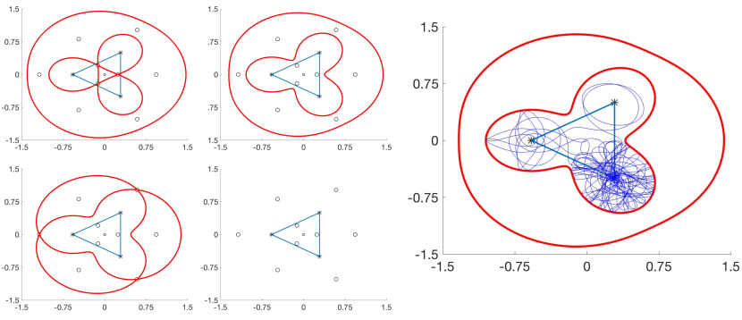
which is called the Jacobi integral. Note that is smooth – in fact real analytic – away from the primaries. The zero velocity curves are defined by fixing a value of the energy and setting to zero. These curves are useful for understanding the structure of the phase space and are illustrated in Figure 2.
As mentioned in the introduction, the CRFBP has exactly , or equilibrium solutions, depending on the values of the mass parameters and . The equilibria are referred to as libration points in the dynamical astronomy literature, and we denote them by for . A typical configuration of these libration points is illustrated in Figure 1, which also illustrates out naming convention. In the present work we are interested in the linear stability of the libration points. We are especially interested in determining the mass ratios where with are saddle-focus – as opposed to real saddle or center center – equilibria. This question is considered from a numerical point of view in Section 2.2.
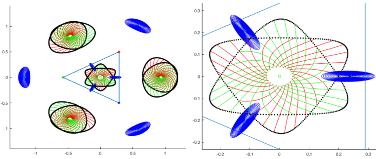
We note that for all values of the masses, with have either saddle center, or center center stability depending on the values of the masses The local two dimensional invariant manifolds attached to all ten libration points are illustrated in Figure 3, for the case of equal masses.
2.2 Saddle foci in parameter space
The CRFBP admits as many as four and as few as zero saddle-focus equilibrium points, depending on the mass ratios. We now consider briefly what happens in between these extremes as the masses are varied. The problem is normalized so that , with , so we have that , and . Considering the 2-simplex in satisfying these constraints, we see that when we have
while for we have
In either case, once we choose and , the value of is determined by
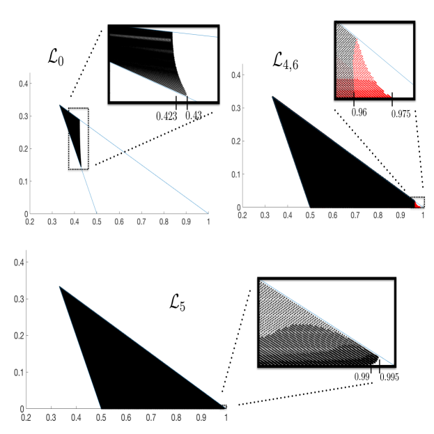
The question is, how does the stability of the libration points depend on the mass ratios? We address the question for each of the points, , as follows. Beginning with the case of equal masses, , we numerically continue each equilibrium to the opposite boundary of the parameter simplex at . Throughout the computation we track the stability of each libration point and label a parameter point with a black dot whenever the stability is of saddle-focus type. The results are summarized in Figure 4. We refer to the curve in the parameter simplex where the stability changes as the Routh-Gascheau curve.
Roughly speaking, we see that when the libration point is a saddle-focus for all allowable values of , . When , the libration point is no longer a saddle, no matter the values of , . The points on the other hand have saddle-focus stability for most parameter values, and only bifurcate after (with a little more robust than except when ). The libration point is the most robust. It maintains saddle-focus stability until . For there are no more saddle foci at all. By reading parameter values off of the frames in Figure 4 we can arrange that the CRFBP has or saddle-focus equilibria. In the sequel we are interested in homoclinic connections for such parameters.
2.3 Two ways to formulate a connecting orbit: phase space geometry and boundary value problems
There are two standard ways to think about connecting orbits and – while they are completely equivalent from a mathematical point of view – in practice they have different advantages and disadvantages. In the following let denote a smooth vector field and let be an equilibrium solution for . We write and to denote respectively the stable and unstable manifolds attached to .
-
•
Analytic definition: If satisfies
for all , and satisfies the asymptotic boundary conditions
then we say that is a homoclinic connecting orbit for .
-
•
Geometric definition: If
and denotes the orbit which passes through , then is a homoclinic connecting orbit for . If the intersection of the manifolds is transverse then we say that is a transverse homoclinic connection.
The analytic definition is recast as a finite time boundary value problem by projecting the boundary conditions onto local stable/unstable manifolds. If are parameterizations of the local unstable and stable manifolds respectively, then we look for and , so that solves the differential equation subject to the boundary conditions
In applications one frequently replaces and by their linear approximations. In Section 3 we review an approach called the parameterization method for computing high order polynomial approximations of the local charts .
Remark 1 (Relative strengths and weaknesses)
One great advantage of the analytic formulation is that, since it is equivalent to a two point boundary value problem, we can utilize the Newton-Method to find very accurate solutions – often on the order of machine precision. The formulation as a boundary value problem also lends itself to numerical continuation schemes, which are very useful for exploring the parameter space. The disadvantages are twofold. First, in this formulation it is necessary to begin the Newton iteration with a fairly good approximate solution and this raises the question: Where do the approximate solutions come from? Second, it is difficult to rule out solutions using the BVP approach.
In the geometric approach there is no need to make a guess. Instead, one moves along the stable and unstable manifolds, and identifies connections by locating intersections in phase space. At the same time, the geometric approach allows one to rule out connecting orbits by showing that a particular region of phase space does not contain any intersections. The difficulty with the geometric perspective is that it provides information only as good as our knowledge of the embeddings of the stable/unstable manifolds. Computing embeddings of invariant manifolds is challenging, and methods tend to decrease in accuracy the farther from the equilibrium they are applied.
The important point, from the perspective of the present work, is that these two approaches complement one another. The geometric formulation is good for locating and ruling out connections while the analytic formulation is good for refining approximations and for continuation with respect to parameters. This suggests the approach of the present work: namely that we use the two formulations in concert, playing the strengths of one against the weaknesses of the other as appropriate.
We remark that in many applications it is convenient to examine the intersections of the invariant manifolds in an intermediate surface of section. This is especially true for two degree of freedom systems as the section intersected with the energy level leads to a two dimensional image which is easy to visualize. Often an appropriate section is suggested by the geometry of the problem, or by the goals of a particular space mission. We refer the interested reader to the works MR1765636 ; MR2163533 ; MR2557453 for examples and fuller discussion.
3 Numerical computation of the stable/unstable manifolds
The results of Section 2.2 show that for most parameter values, the CRFBP has either three or four saddle-focus equilibria – though for some parameters it may have only two, or one, or none. For a given saddle-focus equilibrium with fixed values of the mass parameters, we compute the invariant manifolds in two steps. First we find a high order expansion of an initial local chart containing the equilibrium solution. Then we use a high order Taylor integration scheme to advect the boundary of the initial chart one sub-arc at a time. The second step is repeated until a certain integration time has been reached, or until some error tolerance has been exceeded. Along the way it is sometimes necessary to subdivide boundary arcs in order to manage the truncation errors.
Our computation of the initial chart employs the parameterization method, which is reviewed in Section 3.1. Advection of the boundary uses a Taylor integration scheme similar to the one developed in manifoldPaper1 , but adapted to the problem at hand. Both procedures exploit differential-algebraic manipulations of formal power series, and these manipulations are delicate due to the presence of the minus two thirds power in the nonlinearity of the CRFBP vector field.
One technique for manipulating power series of several complex variables involves automatic differentiation combined with the radial-gradient. This procedure is developed in mamotreto , and is reviewed in Appendix B. Another technique involves appending additional variables and equations to the problem, so that the enlarged field is polynomial and equivalent to the original CRFBP on a certain sub-manifold. This option is discussed at length for the CRFBP in shaneAndJay which also includes a more precise definition of what “equivalent” means here. See also fourierAutomaticDiff , and MR0135589 .
3.1 Parameterization method for the local invariant manifold
We now review the parameterization method adapted to the needs of the present work, namely for a stable/unstable manifold attached to a saddle-focus equilibrium in . Much more general treatment of the parameterization method is found in MR1976079 ; MR1976080 ; MR2177465 . See also the book on this topic mamotreto .
Let denote a saddle-focus equilibrium point. Specifically, we suppose ,
with denotes the stable eigenvalues for , and denotes a choice of associated complex conjugate eigenvectors.
Since the eigenvalues are complex, it is convenient to look for a complex parameterization of a local stable manifold. Let
denote the unit complex polydisc. We look for a parameterization satisfying the infinitesimal conjugacy given by
| (5) |
where , and
Equation (5) is subject to the first order constraints
| (6) |
Note that
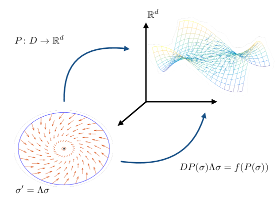
is the push forward of the linear vector field by . The geometric meaning of Equation (5) is illustrated in Figure 5.
Let denote the flow generated by . Any satisfying Equation (5) on also satisfies the flow conjugacy
| (7) |
In particular, if satisfies both Equation (5) and the constraints of Equation (6), then for any it follows that
so that . Combining this with the fact that the image of contains and is tangent to the stable eigenspace at we see that parameterizes a local stable manifold for . Moreover we recover the dynamics on the manifold through the conjugacy.
When the vector field is analytic near , then is an analytic manifold, and it makes sense to look for an analytic chart of the form
with for all . Since we are interested in the real image of the chart we look for a solution of Equation (5) with
for all . This is achieved whenever the power series coefficients of the solution satisfy
| (8) |
for all . The real parameterization is recovered using complex conjugate variables
Elementary proofs of the facts discussed in this section are found for example in shaneAndJay .
3.2 Power series solution of Equation (5)
We describe three methods for computing the power series coefficients of an analytic solution of the invariance equation given in Section 3.1. Combining these methods leads to very efficient numerical methods.
3.2.1 Solution by power matching
Plugging the unknown power series expansion for into Equation (5) leads to
It is shown in MR1976079 (see also the discussion in mamotreto ) that when we match like powers and isolate we are led to an expression of the form
where depends in a nonlinear way on coefficients with . Isolating the variable on the left leads to the homological equations
| (9) |
Remark 2 (The formal solution is well defined)
. Observe that Equation (9) is linear in and has a unique solution as long as is not an eigenvalue of . But , and since any remaining eigenvalues are assumed to be unstable, we have that is never an eigenvalue of . Hence the matrix on the left hand side of the homological equation (9) is invertible for all .
Given any first order data as in the constraint Equations (6), the homological equations are uniquely solvable to all orders and the corresponding formal series solution of Equation (5) is well defined. Since each Taylor coefficient is uniquely determined by the homological equations (9), it follows that the formal series solution is unique up to the choice of the scalings of the eigenvectors in Equation (6). Solving the homological equations recursively to order provides a polynomial chart which approximately parameterizes the local stable manifold.
3.2.2 A Newton scheme
A quadratic convergence scheme for Equation (5) is obtained as follows. Define the nonlinear operator
where is the CRFBP vector field, and note that a zero of is a solution of Equation (5). Moreover we note that, at least formally, the Fréchet derivative is given by
In fact this is the correct Fréchet derivative of when for example we consider defined on a Banach space of analytic functions, see MR1976079 ; MR2177465 ; MR2966749 .
Choose an approximate zero of , and define the sequence
where is the formal series solution of the linear equation
| (10) |
If is a good enough approximate solution of Equation (5) we expect to converge quadratically to a zero of . The linear operator non-constant coefficient, and Equation (10) may be solved recursively via the following power matching scheme. Define
and
Here , and are complex valued matrices for all . Plugging these series expansions into Equation (10) leads to
or, upon matching like powers,
for all . We note that the sum contains one term of order , appearing when and . That is
Let
Then we use to extract terms of order from the sum and write the equation for as
Recall that , so that rearranging terms leads to the linear equations
| (11) |
for . Since the right hand side of Equation (11) is exactly the right hand side appearing in the homological equations (9) of Section 3.2.1, arguing as in Remarks 2 and 3 shows that the Equations of (11) are uniquely solvable for all just as before, and that the resulting power series coefficients have the desired symmetry. Then this Newton scheme is well defined on the space of formal power series.
3.2.3 A pseudo-Newton scheme
While the Newton scheme of the previous section converges rapidly (in the sense of the number of necessary iterations), solving the required non-constant coefficient linear equations are expensive. In this case the overall computation may be slow just because of the cost of computing the individual corrections. The iterations can be speed up as follows.
First, we note that
and we define a new iterative scheme
where is a solution of the constant coefficient linear equation
On the level of power series, this equation becomes
and matching like powers yields the linear equations
These homological equations uniquely determines the coefficients , and have the virtue of being “diagonal” in Taylor coefficient space. In practice we find that the pseudo-Newton scheme requires more iterates than the Newton method to converge. However, a single iteration step is much faster and for reasonable values of the pseudo-Newton method is faster overall. We discuss this further below.
Remark 4
In practice the linear approximation of by the eigenvectors provides a good initial guess for the Newton and pseudo-Newton schemes, especially when computations are started “from scratch”. However, within the context of calculations based on parameter continuation, we will take as the high order parameterization from the previous mass values.
Indeed, it seems that the best results are obtained by a “hybrid” approach. That is, we compute an initial guess by recursively solving Equation (9) to some fixed order, . Then, we refine this approximation via the Newton or pseudo-Newton scheme to obtain a polynomial approximation to order, . The runtime performance for this hybrid approach is recorded in Table 2.
Remark 5 (Quantifying the errors)
Suppose that the polynomial
is an approximation solution of Equation (5). One way to measure the quality of the approximation is to measure the defect associated with defined by the quantity
This quantity could be approximated by evaluating on a mesh of points in . On the other hand, we can use the fact that for power series on the unit disk we have the bound
where the infinite sum can be approximated by a finite sum. Then another useful a-posteriori indicator is obtained by choosing an and computing the quantity
where are the power series coefficients of , and are the coefficients of . Of course this bounds also the real image of .
If is a polynomial of order then we take . If is not a polynomial, then the power series for has infinitely many terms even though is polynomial. Then we choose somewhat arbitrarily. Note that are zero when , so that eventually the sum involves only the coefficients of the composition.
Yet another useful error indicator is obtained by considering the dynamical conjugacy of Equation (7). Since the true solution satisfies the dynamical conjugacy exactly we consider also the quantity defined by
To approximate this quantity we fix and let denote a numerical integrator and , be a mesh of the complex circle so . Define the indicator
Error bounds for a number of example computations are recorded in Table 1.
| defect | conj error | machine eps | |||
|---|---|---|---|---|---|
| 18 | |||||
| 5,855 | |||||
| 68 | |||||
| 73 | |||||
| 356 | |||||
| 73 | |||||
| 1036 | |||||
| 73 | |||||
Remark 6 (Eigenvector scaling and coefficient decay)
Solutions of Equation (5) are only unique up to the choice of the scalings of the eigenvectors and this freedom is exploited in our numerical algorithms. Indeed, this is the reason we can always take our domain to be the unit disk. The results in Table 1 describe the dependence of the numerical errors on the approximation order and the eigenvector scalings. These numerical experiments lead to the following heuristic. If we scale the eigenvectors so that the final coefficients – that is the -th order coefficients of – are on the order of machine epsilon, then we obtain a-posteriori errors on the order of machine epsilon.
| recursion | Newton | pseudo-Newton | ||||
|---|---|---|---|---|---|---|
| (sec) | (sec) | (sec) | ||||
| (sec) | (sec) | (sec) | ||||
| (sec) | (sec) | (sec) | ||||
| (sec) | (sec) | (sec) | ||||
| (sec) | (sec) | (sec) | ||||
| (sec) | (sec) | (sec) | ||||
| (sec) | (sec) | (sec) | ||||
| (sec) | (sec) | (sec) | ||||
| (sec) | (sec) | (sec) |
3.3 Integration of analytic arcs
In Section 4 we present a scheme for computing an atlas for the stable/unstable manifolds which relies on integrating analytic arcs of initial conditions by the flow generated by . We describe this integrator in terms of power series expansions. Let us assume that is an analytic arc with power series expansion
Denote the formal series expansion
Here, we use the variables in place of to emphasize the intuition that corresponds to the “spatial” parameterization along the initial data, and corresponds to the “time” parameterization along the flow. In other words, we consider as the solution of the parameterized family of initial value problems
Substituting the formal series into this IVP and matching like powers leads to the recursion relations
which allow us to compute the coefficients of to arbitrary order using the same methods described in Section 3.2. We also note that the precision of these formal series computations depend on convergence and domain decomposition of these series expansions which has not been addressed and will also be taken up in the following section.
4 Building an atlas for the local stable/unstable manifold
In this section let denote an invariant stable/unstable manifold for a saddle-focus equilibrium, . Our goal is to describe an algorithm for producing an atlas of chart maps which parameterizes a large portion of the invariant manifold. The union of the images of these maps is a piecewise parameterization of a -dimensional subset of . Our procedure is iterative and at each step outputs a (strictly) larger piecewise parameterization.
It is important to emphasize that our computations are carried out only to finite order. In particular, the charts described in this section are analytic functions of two complex variables. However, in practice we fix , and for each chart we compute a finite polynomial approximation of order . Nevertheless, throughout this section we denote these analytic charts and their polynomial approximations using the same notation. We end this section by outlining methods for reliably, efficiently, and automatically computing these atlases. This includes algorithms for estimating and controlling truncation errors, identifying Taylor series blowup, domain decomposition, and stiffness.
4.1 Iterative method for computing charts
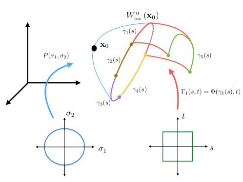
Before elaborating on the technical details of our method we briefly describe the overall strategy. Starting from the parameterized local invariant manifolds obtained via methods described in Section 3.1, we want to build an even larger representation of the manifold. There are many ways to grow such a representation. We could for example simply integrate a collection of initial conditions meshing the boundary of the parameterization. However, as is well known, the exponential separation of initial conditions will force these orbits apart and eventually degrade the description of the manifold. Instead we mesh the boundary into a collection of one dimensional arcs and advect each of these under the flow. Propagating these arcs maintains the fidelity of the representation, and leads to new “patches” of the manifold.
Since the initial chart is parameterized by a high order polynomial, we would like the same representation for new charts. To this end we develop a high order Taylor integration scheme which applies to analytic arcs of initial conditions. This results in a power series representation of the flow of a boundary arc, and we take this as our next chart. After advecting each one of the boundary arcs we have a new and strictly larger representation of local stable/unstable manifold. The idea is illustrated in Figure 6.
After one step of this procedure we have moved the boundary of the local invariant manifold. In some cases, the image of the advected arc undergoes excessive stretching due to the exponential separation of initial conditions. This stretching in phase space is matched by a corresponding blow up in coefficients of the Taylor expansion, and the computations become numerically unstable.
This problem is overcome by occasionally remeshing the boundary of the atlas. This comes at a cost of increasing the number of charts in the next step of the algorithm. Hence, efficiently computing large atlases while controlling numerical error requires automatic algorithms for managing the growth of the power series coefficients, deciding how long to integrate each individual arc, and deciding when and how to subdivide the new boundaries. These topics account for much of the technical details which follow.
4.1.1 The initial local manifold
The first step in our algorithm is to compute a polynomial approximation of the local parameterization, either by directly solving the homological equations or by iterating the Newton or pseudo-Newton schemes described in Section 3.1. Let be a solution of Equation (5), and denote the unit polydisc in . Recall that is analytic, and that is flow transverse. In particular, serves as our initial local parameterization, and we refer to it as a generation interior chart and we write .
In practice, we compute to order with chosen by applying the heuristic methods discussed in Section 3.2. This chart is represented in the computer as a polynomial in two complex variables of total degree . The truncation error of this approximation is controlled directly by choosing the eigenvector scaling as described in Remark 6, and in practice, is on the order of machine epsilon.
4.1.2 The initial manifold boundary
With in hand, we fix and subdivide into -many analytic segments, each of which has the form, , for . We parameterize by defining and we refer to as a lifted boundary. Note that for each , and is a flow transverse arc since is a dynamical conjugacy and the image of is transverse to the linear flow. Now, we define the generation boundary to be
and refer to each as a generation boundary chart.
4.1.3 The next generation
Now, we apply the high-order Taylor advection described in Section 3.3 to grow a larger local manifold denoted by . Specifically, for , we choose , and our advection algorithm takes as input and produces a chart, which satisfies
In other words, parameterizes the advected image of under the flow over the time interval . These new charts are referred to as generation interior charts which we add to our atlas to obtain the first generation local parameterization
Note that and since is flow transverse, we have is a strict subset. In fact, transversality of implies the stronger condition that i.e. the manifold has grown through every point on the previous boundary.
Remark 7 (Time rescaling)
In this description, serves as a time-rescaling of the flow. This allows direct control over the truncation error (in the time direction) and is analogous to the eigenvector scaling for the initial parameterization described in Remark 6. However, choosing this time-rescaling is typically more difficult than choosing the eigenvector scaling and we postpone the discussion of this problem to Section 4.2.1.
Once the generation interior charts are computed by advection, the generation boundary arcs are now obtained by evaluation of the time variable. In particular, for , the evaluation, is a flow transverse arc segment. We perform spatial rescaling as needed (see Remark 8 below) to obtain the next generation boundary arcs, where for some and
is flow transverse. The advection and evaluation algorithms are then iterated to increase the number of charts in the atlas. The step in the iteration chain has the form
where is parameterized by -many interior charts (polynomials in both the space and time variables), is parameterized by -many boundary charts (polynomials in the space variable only), and .
If we stop iteration, say at the , then the final atlas,
is a collection of -many analytic charts is a piecewise parameterization a portion of the invariant manifold.
Remark 8 (Spatial rescaling)
The parameters, , control the number of boundary subdivisions, and therefore, allow direct control over scaling in the spatial direction. As in the time-rescaling problem, choosing these parameters effectively is a nontrivial problem which we take up in Section 4.2.2.
4.2 Convergence, manifold subdivision, and numerical integration
Thus far, we have ignored the issue of convergence for our formal power series computations. The best method for studying this issue is to combine rigorous numerical computations with a-posteriori analysis and obtain a proof of the existence of an analytic solution and explicit error bounds on the polynomial approximation. Rigorously validated numerical methods for invariant manifold atlases are described in detail in manifoldPaper1 ; shaneAndJay . In the present work we explore the utility of invariant manifold atlases as a purely numerical tool, and trade the computer assisted proof of rigorous error bounds for improved runtime performance.
In the absence of a rigorous validation scheme we develop more heuristic checks to insure the reliability of the computations. More precisely, we must automatically identify and fix numerical accuracy issues related to numerical Taylor integration. This amounts to rescaling our Taylor coefficients whenever the decay in either space or time becomes too slow. However, this is less straight-forward than the eigenvector rescaling for the initial local parameterization described in Remark 6. In particular, it is helpful to consider the rescaling in space and time “directions” separately.
4.2.1 Time-stepping
Recall that at the saddle-focus equilibrium, the stable/unstable eigenvalues occur in complex conjugate pairs. In particular, both eigenvalues in each pair have equal real parts. It follows that identically re-scaling each pair of eigenvectors is the ideal strategy. In fact, this strategy is also necessary and sufficient to ensure that the initial parameterization is real-valued, see parmChristian . Moreover, in the general case of a hyperbolic equilibrium, the real part of each eigenvalue is a measure of the expansion or contraction rate in the direction of its associated eigenvector. Thus, in cases for which they are not equal, the real parts are still explicitly known and the eigenvectors are scaled proportional to these rates.
On the other hand, all but the initial chart in our atlas is obtained via our advection scheme. In this case, neither the expansion/contraction rates, or their directions are explicitly known. Obtaining these estimates would require solving for the (spatial) derivative of the flow on each chart. For a general vector field defined on , this amounts to increasing the phase space dimension of our ODE solver from , to , which would significantly reduce the size of each manifold which is computationally feasible to produce.
Instead, we take an approach similar to manifoldPaper1 , which describes heuristics for rescaling time and space independent of one another. Specifically, we adopt a time-rescaling which ensures that the norm of the “coefficient” (with respect to ) for each chart, is less than machine epsilon. Note that for a classical IVP this coefficient is of course just a scalar. However, in our case the coefficient is actually an analytic function of the spatial variable, represented as a power series and the norm of this coefficient is measured using the norm. This is made more precise in the following section.
This choice is highly conservative, which gives us tight control over the truncation error in the time direction. On the other hand, the spatial rescaling in the present work deviates from the scheme presented in manifoldPaper1 and is detailed in Section 4.2.2.
4.2.2 Manifold subdivision
Next, we describe the spatial-rescaling scheme which we refer to as manifold subdivision. We assume that the time-rescaling described in the previous section has been carried out on each chart, and our interest is in rescaling each boundary arc to control truncation errors accumulating in the “space direction”. This is equivalent to subdividing a manifold since it is reasonable to assume the rescaling will always shrink the domain. Thus, a single boundary arc will give rise to multiple subarcs defined on reduced domains.
To be more precise, we let denote the collection of real-valued, analytic functions defined on , and let denote the collection of real-valued sequences. We define the Taylor transform, , to be the mapping which sends an analytic function to its sequence of Taylor coefficients centered at . Specifically, if has the Taylor expansion,
then . Now, we equip with the -norm defined by
and we note that elements of with finite norm form a closed sub-algebra denoted as
and we write when we want to emphasize that (i.e. we write for the norm when is finite).
We remark that our error analysis is carried out using the -norm due to the efficiency of computing this norm for polynomials. However, if is a numerical approximation, then the errors we are interested in are of the form
We are justified in using the norm due to the well known result that .
Now, suppose and assume that . Since is a non-linear flow, a typical arc segment undergoes rapid deformation and stretching when advected. This implies that for a single step in our algorithm with the general form,
we expect both the arc length and curvature of to be larger than for . On the level of Taylor coefficients, this statement about deformation/stretching says that if , then in general we expect . The relationship between this norm and the truncation error implies that advecting an arc adversely impacts the propagation error.
To see this, we recall that in practice our computation stores a truncated polynomial approximation for in the form . In order that is a “good” approximation (in the topology), must be “small” for each . These higher order terms correspond to the truncation error for and primarily arise from two sources. One source which we can not control (once is fixed) is the truncation error associated with . However, by inspection of the Cauchy product formula in Equation (19), it is clear that the polynomial coefficients stored for also contribute to this truncation error for after applying the nonlinearity. We refer to these contributions as spillover terms.
This observation implies that for to be a good approximation, we must also require that is “small” for each where depends on the degree of the nonlinearity. This motivates the following heuristic method for controlling truncation error for propagated arcs. We begin by assuming that has approximately geometric decay. Specifically, we expect that there exists some such that the tail of the series defined by decays faster than the geometric series with ratio . In this case, the truncation error is of order . Now, fix , and we define the tail ratio for by
| (12) |
Evidently, is small whenever “most” of the weight of is carried in the first -many coefficients. It follows that if is sufficiently small, then under the action of a nonlinear function, , the spillover terms for remain small. Of course, small is dependent on context and in particular, choices for as well as thresholding values for are problem specific. In the present work, we prove it is always possible to control .
Remark 9
Strictly speaking, for the CRFBP we have where each is a coordinate for the boundary chart. Similarly, , and thus the discussion in Section 4.2.2 thus far is technically not applicable. However, our restriction to scalar valued functions is justified by the fact that if , then defining
makes into a normed vector space. This choice of norm gives us the freedom to restrict the discussion of remeshing and tail ratios to scalar valued functions.
Next, we describe our scheme for controlling the tail ratio. This algorithm takes a polynomial representation for , defined on as input, and returns a list of polynomials, , as outputs. The key point is that these polynomials are also defined on , and they can be chosen such that is arbitrarily small for . In this work, we assume the output polynomials are specified as coefficient vectors of length (i.e. the same degree as the input), however this is not required.
This gives rise to an additional remeshing step in our algorithm which is performed as needed after an evaluation step and prior to an advection step leading to an updated schematic
In the remeshing step, the tail ratio for each boundary arc from the previous step is computed and checked against a threshold. Boundary arcs which exceed this threshold are flagged as poorly-conditioned, and subdivided into smaller subarcs which satisfy the threshold. The collection of resulting subarcs and well-conditioned arcs from the previous step is passed to the advection step where each results in a separate chart.
Before proving this threshold can always be satisfied, we describe the subdivision algorithm. As noted in Remark 9, it suffices to consider a single coordinate for a parameterized boundary arc. Thus, we assume is analytic with Taylor series
and fix a subinterval, . Define the constants
| (13) |
and define by
| (14) |
Then is a parameterization for the arc segment parameterized by restricted to . In fact, is the Taylor series for after re-centering at and re-scaling by which satisfies the functional equation
| (15) |
Moreover, the mapping is a linear transformation on , and in particular, if for all , then for all also. Now, we prove that we have explicit control over the tail ratio for .
Proposition 1 (Controlling tail ratios)
Suppose is analytic, fix , , and let . Then there exists such that where is the truncation to order for defined by as in Equation (14).
Proof
Define to be the Taylor polynomial obtained by truncating the Taylor series for to order . For , define the usual -norm on to be
Since is a polynomial, we have the bound
In particular, for any , we have , for , and we define
It follows that
Now, let be defined as in Equation (14). Recall that is also analytic on and by differentiating Equation (15) we have the derivative formula, , for all . By Taylor’s theorem, we obtain another explicit formula for given by
and we note that does not depend on . We have the estimate for the tail ratio of :
which completes the proof.
Proposition 1 establishes the fact that we may re-parameterize on subintervals of with width, , and that as the tail ratio also approaches zero. We note that does not depend on the subinterval, and therefore, for a fixed the number of required subarcs is finite. In particular, no more than subarcs are required. To summarize the usefulness of this result, we present the following algorithm for controlling the spatial truncation error which was implemented for the atlases in this work.
-
1.
Fix a threshold , a cutoff , and . The threshold and cutoff are both chosen based on the alignment of with the flow, the degree of the non-linearity in , and the truncation size. In practice, these are problem specific choices which require some ad-hoc experimentation in order to balance computational efficiency and truncation error.
-
2.
Following each evaluation step in our algorithm, a boundary arc has the form which is stored in the computer as a polynomial approximation, . If , continue to the advection step.
-
3.
If , specify a partition of into -many subintervals by choosing their endpoints, . Apply the formula in Equation (14) to obtain where for , where and .
-
4.
Each resulting subarc which satisfies the tail ratio threshold passes to the advection step. Subarcs which violate the threshold are subdivided again by repeating step 3. By Proposition 1, this condition is eventually met for every subarc and the algorithm proceeds to the advection step.
4.2.3 Stiffness
The final numerical consideration which we address is the stiffness problem. We recall that the CRFBP vector field is analytic away from the primary masses which correspond to singularities of Equation (3). Since this system is Hamiltonian, any trajectory which collides with one of these primaries must blow up in finite time. However, smooth trajectories may pass arbitrarily close to these primaries and as they do, the velocity coordinates, , become arbitrarily large.
Recall that a single boundary arc, , is a parameterized manifold of initial data. Then its advected image, , is a parameterized bundle of trajectory segments. For any , parameterizes the trajectory passing through over the (non-scaled) time interval, .
Now, suppose that for , the trajectory through passes “close” to a primary at time . Then, we have
Recalling our time-rescaling algorithm described in Section 4.2.1, it is clear that controlling truncation in the time direction will require taking increasingly shorter time-steps. Of course this is not surprising, however, the difficulty arises from the fact that other choices of often correspond to trajectory segments which remain far away from the primary and our time-rescaling is applies uniformly on . Hence, the advection of the entire boundary chart is slowed dramatically whenever any portion of its image approaches a primary. We refer to these charts as stiff. Obviously, this is a major problem for our “breadth-first” approach for computing the manifold atlas. Namely, the integrator gets stuck on the stiff charts causing the computation to stall.
A naive method for dealing with this is to define the speed for a boundary chart which is a parameterized curve of the form, , , by
| (16) |
set a threshold, , and cease advection of whenever . While this fixes the problem of computational efficiency, we also lose large portions of the manifold which remain far from the primaries. Instead, we leverage the manifold subdivision procedure which was already introduced in Section 4.2.2 to modify the naive algorithm in order to retain these portions of the manifold as follows.
-
1.
Fix a maximum speed threshold, . For each boundary chart, , present after the evaluation step, check that and if so, continue to the remeshing step.
-
2.
If , write and compute
Since are polynomial approximations, this set is a finite collection of roots of a polynomial which we denote by, .
-
3.
For , check that holds on and if so, compute as in Equation (14) and continue to the remeshing step. Subintervals which fail this check are discarded.
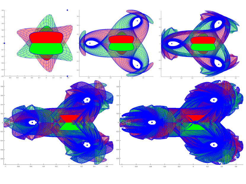
To summarize, our algorithm identifies regions of the manifold boundary which pass close to a primary by checking the maximum speed. Regions which exceed a threshold are cut away while regions of the nearby boundary continue to be advected. The cut regions cause the apparent holes punched out around each primary in the manifold plots, such as Figures 7 and 8.
4.3 Computational results: manifold atlases for the triple Copenhagen problem
Performance results for atlas computations at the libration points and are given in Tables 3 and 4 respectively. The computations are performed for the case of equal masses, that is for the triple Copenhagen problem. The tables report the advection time – that is the number of time units the boundary of the local parameterizations are integrated – as well as the time required to complete the computations and the number of polynomial charts comprising the atlas. All computations were performed on a MacBook Air laptop running Sierra version 10.12.6, on a 1.8 GHz Intel Core i5, with 8 GB of 1600 MHz DDR3 memory.
| Integration Time | Run Time (both manifolds) | # Stable Charts | # Unstable Charts |
|---|---|---|---|
| seconds | 39 | 39 | |
| seconds | 146 | 146 | |
| seconds | 497 | 497 | |
| minutes | 700 | 700 | |
| minutes | 1579 | 1579 | |
| minutes | 3530 | 3493 | |
| minutes | 9372 | 9295 |
| Integration Time | Run Time (both manifolds) | # Stable Charts | # Unstable Charts |
|---|---|---|---|
| seconds | 124 | 124 | |
| seconds | 216 | 216 | |
| minutes | 487 | 487 | |
| minutes | 634 | 634 | |
| minutes | 1466 | 1466 | |
| minutes | 2899 | 2899 | |
| minutes | 4983 | 4751 |
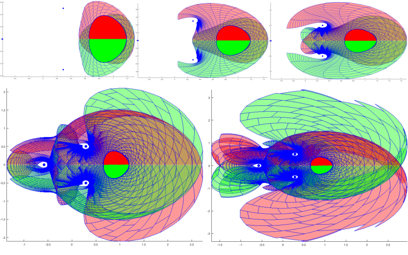
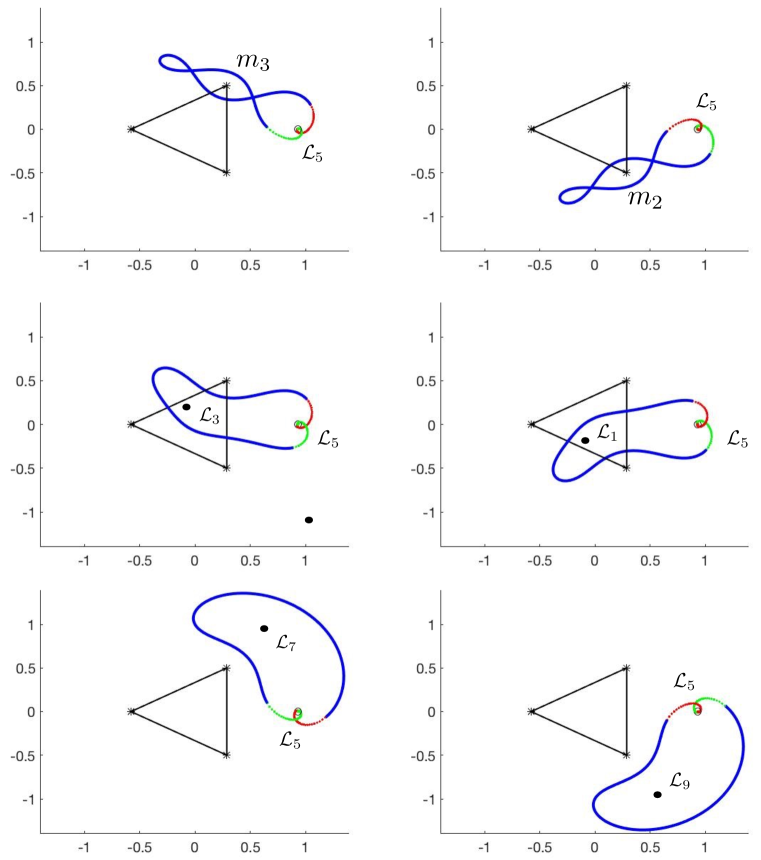
The resulting atlases for and are illustrated in Figures 7 and 8 for various integration times. The boundaries for the charts are also shown, making it clear that the computational effort goes up dramatically near the primaries. Note that the chart boundary lines running out of the local parameterizations are actual orbits of the system and hence give a sense of the dynamics on the manifold. The pictures provide some insight into the dynamics of the problem, however, their complexity illustrates the need for more sophisticated search techniques in order to extract further useful qualitative information from the atlases.
5 Homoclinic dynamics in the CRFBP
In this section we discuss connecting orbits found for the symmetric case by searching the manifold atlases computed in the previous section.
5.1 Mining the atlases
Assume we have computed atlases, , for the stable/unstable manifolds of . We are interested in “mining” the chart data to find transverse connections. Since each atlas is stored as a collection of polynomial charts, it suffices to identify pairwise intersections between stable and unstable charts. Thus, throughout we assume is a pair of charts which parameterize a portion of the stable/unstable manifold. We write denote the scalar coordinates of each chart. The following theorem whose proof can be found in shaneAndJay provides a computable condition for verifying transverse intersection of a pair of charts.
Theorem 5.1
Define by
and suppose satisfies . If and have the same sign, then is homoclinic to . Moreover, if is nonsingular and if (where is the CRFBP energy), then the energy level set is a smooth -manifold near and the stable/unstable manifolds of intersect transversally in the energy manifold.
We emphasize that Theorem 5.1 provides a computable condition for verifying a transverse intersection using rigorous numerics. However, we will use the same theorem to detect transverse intersections in the purely numerical setting of this paper. This is made explicit in the following algorithm utilized in the mining scheme for all results in the present work.
Assume, are as defined in Theorem 5.1. Apply Newton’s method to find an approximate root of . Let denote an approximate solution with , and check the following conditions:
-
1.
, and are both “far” from 0.
-
2.
, and have the same sign.
If condition 1 holds without condition 2, then these charts are non-intersecting. In this case, these charts lie on separated portions of the stable/unstable manifolds which are symmetric with respect to the fourth coordinate. We refer to these as “pseudo-intersections”. On the other hand, if both conditions hold, then we conclude from Theorem 5.1 that we have numerically found a transverse homoclinic for passing through .
Note that condition 1 serves two purposes in this setting. First, it serves as an easily computable condition for checking that as required in the theorem. This follows by noting that
so it follows that is satisfied automatically whenever condition 1 is satisfied.
In addition, condition 1 gives us some confidence that the sign difference from condition 2 holds due to transversality of the homoclinic, as opposed to numerical error. Indeed, if condition 1 is not satisfied, then , and take values near zero in which case sign errors for either coordinate are likely due to integration errors. In this case, even if condition 2 is satisfied we are unable to trust the result, hence unable to conclude whether the zero of corresponds to a transverse intersection or a pseudo-intersection. Fortunately, this situation can be remedied as discussed in Remark 11. As a result, we are free to choose our threshold for what is meant by “far” in the statement of condition 1 very conservatively which leads to a great deal of confidence that our mining algorithm returns only transverse homoclinic orbits.
We further increase our confidence in the approximate connection by using it as the input for a BVP solver based on Newton’s method, which allows us to refine our approximation to nearly machine precision and it is the BVP formulation to which we then apply continuation methods. Every connection reported in this section has been so certified and none of the connections identified from the mining algorithm had a BVP which failed to converge. In other words, the mining algorithm did not return any false homoclinics.
5.2 Efficient atlas mining
It is not desirable to check every pair of charts from each atlas using the above procedure, and we introduce two methods which significantly reduce the number of chart pairs which must be checked via the Newton intersection scheme based on Theorem 5.1.
5.2.1 The box approximation
The first method for improving the mining efficiency is to apply a coarse preprocessing step to each pair of charts which must be compared. The main idea is based on the fact that for most pairs of charts which do not intersect, these charts will “obviously” not intersect in the sense that their images in phase space will be very far apart. We exploit this using a fast algorithm for identifying many such pairs, and in this case skip the slower Newton-based intersection attempt.
To be more precise, consider an arbitrary polynomial defined by
We define the box for to be
The significance of is that we have the bound
or equivalently, for all . Analogously, we extend this to higher dimensions component-wise and apply this to geometrically rule out pairs of charts which can not intersect because their images are “well separated”. Specifically, consider a pair of stable/unstable charts
which have boxes described by rectangles in and satisfying , and . Then, if the set distance, is large enough, we can conclude that do not intersect.
Using boxes has two advantages. The first is that computing and checking boxes for pairwise intersections is much faster than our Newton-like intersection method. This is due to the fact that for each coordinate the box radius, , is equivalently computed as
which is extremely fast to compute using modern implementations. Determining whether two boxes intersect or not is also fast due to efficient interval arithmetic libraries such as the INTLAB library for MATLAB Ru99a which was utilized in our implementation.
The second advantage is that an box is typically a very coarse enclosure for the true values of . This “problem” is often referred to as the data-dependence problem or the wrapping effect. In our situation however, we consider the coarseness to be a feature since it makes our numerical estimates more conservative. Thus, we are able to rule out many pairs of charts which clearly do not intersect without eliminating false negatives.
In practice, a single pairwise box intersection check is approximately 1,000 times more efficient than the Newton-based scheme and this method rules out around 90 percent of non-intersecting chart pairs. Moreover, the box for each chart can be computed only once during the atlas construction and stored. This leaves the cost of a single box intersection check as the only significant computational operation.
Finally, we remark that once boxes have been computed and stored for each chart in both atlases, one can make careful use of the triangle inequality to reduce the computation even further. This provides roughly an additional order of magnitude improvement in the efficiency of our algorithm which could be crucial to the feasibility of mining extremely large atlases. However, we took limited advantage of this fact in the present work.
5.2.2 Fundamental domains
The other main source of efficiency gain in our algorithm relies on using the dynamics explicitly. Recalling our notation in Section 4, assume is the stable manifold atlas which we have computed to include the generation and let denote the generation local stable manifold. Then, is a fundamental domain for . In other words, if is any orbit which satisfies and if , then there exists such that . Of course, the same claim holds for the unstable manifold. Taken together, if we assume we have computed the unstable manifold, , up to the generation, then we have the following observation.
Proposition 5.2
Let be a transverse homoclinic to . Then for all . Let denote the generation sequence of local stable/unstable manifolds. Then exactly one of the following is true.
-
•
There exists and , such that and is constant for all pairs which satisfy this property.
-
•
There exists such that for all , and , we have
Proposition 5.2 says that any transverse homoclinic for satisfying the second condition is a connection which does not intersect in the atlases which we have computed. Restricting to those that do, this proposition says that there is a “first” generation for both the stable and unstable atlases for which the connection will appear.
The significance of this situation is that we need only do pairwise comparisons between stable/unstable charts one generation at a time. Thus, the computational complexity for mining intersections between the two atlases has computational complexity of order where are the sizes of the largest stable/unstable generations respectively. This is a dramatic improvement over the naive solution of checking every pair in both atlases which has complexity on order .
Remark 10
We note that often the atlases we compute in practice do not technically satisfy the fundamental domain property. This is due to the fact that sections of manifold boundary which pass near a primary are “cut out” as described in Section 4.2.3. Nevertheless, this has no impact on our mining algorithm. Specifically, each generation is still a fundamental domain for the subset of the global manifold which satisfies the speed constraint. Thus, mining for connections via “leapfrogging” through pairwise generations is still assured to find all connections which are present in the computed atlases, and therefore, all connections which satisfy the speed constraint.
Remark 11
The result in Proposition 5.2 gives rise to a natural mining algorithm. Namely, at each generation, all chart pairs are compared and transverse intersections are identified. It follows that once a transverse intersection is identified, then the next/previous generation must also contain an orbit segment corresponding to the same homoclinic. Hence, in addition to gaining a computational speedup, exploiting the fundamental domain property also ensures that all homoclinics identified are distinct. This follows from the existence of the minimum value for in Proposition 5.2.
Furthermore, this observation yields a method of resolving the ambiguous case in which the Newton-intersection method finds a zero for but condition 1 from Section 5.1 is not satisfied. Specifically, if and , then we may follow the suspected intersection through earlier/later generation charts until the sign condition can be verified or refuted in appropriate predecessor/successor charts. Lastly, we mention that by storing “parent/child” information about the charts in the atlas, we can perform the search just described in post-processing.
| Connection | Connection Time | Letter or Word |
|---|---|---|
| st | ||
| nd | 2.331 | |
| rd | 4.198 | |
| th | 4.520 | |
| th | 4.715 | |
| th | 5.643 | |
| th | 6.132 | |
| th | 6.132 | |
| th | 6.583 | |
| th | 6.627 | |
| th | 6.628 | |
| th | 6.684 | |
| th | 6.760 | |
| th | 6.846 | |
| th | 7.009 | |
| th | 7.336 | |
| th | 7.038 | |
| th | 7.038 | |
| th | 7.490 | |
| th | 8.119 | |
| st | 8.125 |
| Connection | Connection Time | Letter or Word |
|---|---|---|
| nd | 8.125 | |
| rd | 8.296 | |
| th | 8.448 | |
| th | 8.453 | |
| th | 8.453 | |
| th | 8.499 | |
| th | 8.499 | |
| th | 8.583 | |
| th | 8.614 | |
| st | 8.732 | |
| nd | 8.794 | |
| rd | 8.937 | |
| th | 8.953 | |
| th | 8.953 | |
| th | 9.065 | |
| th | 9.340 | |
| th | 9.88 | |
| th | 9.444 | |
| th | 9.495 | |
| st | 9.579 | |
| nd | 9.579 |
| Connection | Connection Time | Letter or Word |
|---|---|---|
| st and nd | and | |
| rd and th | and | |
| th and th | and | |
| th | 6.028 | |
| th | 8.204 | |
| th | 8.331 | |
| th | 8.456 | |
| th | 8.917 | |
| th | 8.934 | |
| th | 9.156 |
| Connection | Connection Time | Letter or Word |
|---|---|---|
| th | 9.324 | |
| th | 9.363 | |
| th | 9.387 | |
| th | 9.429 | |
| th | 9.429 | |
| th | 9.487 | |
| th | 9.487 | |
| st | 9.554 | |
| nd | 9.554 | |
| rd | 9.629 |
5.3 The symmetric case: locating, refining, and classifying, connections
We now describe the homoclinic mining procedure in the case of the triple Copenhagen problem. Assuming we have computed stable/unstable atlases denoted by respectively. Each atlas is of the form described in Section 4 i.e. each atlas is a union of chart maps having the form, with .
We begin with a lemma to motivate the choice to grow each atlas in the symmetric case and then do continuation as opposed to growing the atlas for non-symmetric cases.
Lemma 1
Assume is the symmetric CRFBP vector field i.e. and define two linear maps, by where is the matrix given by
then is a rotational conjugacy for and for all . In particular, if parameterizes a homoclinic orbit for , then are parameterizations for two additional, distinct “symmetric” homoclinic orbits for . Moreover, if parameterizes a homoclinic orbit for , then and parameterize symmetric homoclinics for and .
The proof of Lemma 1 is included in Appendix A. The significance of this symmetry is the fact that global stable/unstable atlases for the triple Copenhagen problem can be separated into 3 distinct equivalence classes where for , the equivalence relation is satisfied if and only if . Thus, each atlas is obtained by advection of only a single representative for each class. In other words, in the equal masses case, we only need to advect of each initial parameterization boundary to obtain the entire atlas. Specifically, we define
and we globalize only to obtain a partial atlas, . We can then access the full global atlas by applying to each chart in and we set
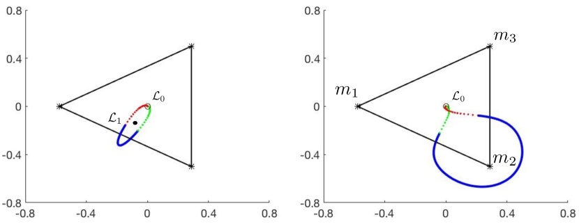
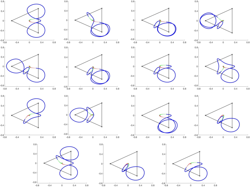
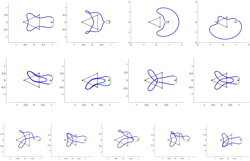
The advantage is a -fold increase in computational efficiency for the atlas computation, and a -fold improvement in efficiency for the atlas mining scheme. Applying the procedure for the triple Copenhagen problems results in the connecting orbits illustrated in Figure 9. These results are further described and classified in the next section.
5.3.1 Quantitative/qualitative classifications of the homoclinic orbit set at
Suppose is an equilibrium solution and a local stable/unstable manifold. Let be an orbit homoclinic to , and suppose that is the elapsed time from when passes through the boundary of the local unstable manifold to when passes through the boundary of the local stable manifold. Observe that if and if the vector field is inflowing/outflowing on the boundaries of respectively, then is well defined.
When the local parameterizations intersect only at , it makes sense to talk about the “shortest” connection time,” the “second shortest” connection time, and so on. This natural ordering on connection times provides a useful observable for classifying homoclinic connections relative to fixed local stable/unstable manifolds. Generically, we expect a one-to-one correspondence between connecting orbits and connection times, though this expectation will fail in the presence of symmetries as seen below.
In the CRFBP, when we “mine” the stable/unstable atlases for connecting orbits and order them by connection time we see something interesting. In each of the cases we studied, the shortest homoclinic orbits appear to organize the longer connections. Informally speaking, we find that a small number of short homoclinic orbits serve as a sort of alphabet of “letters”, and the longer connections can be roughly identified as “words” in this alphabet.
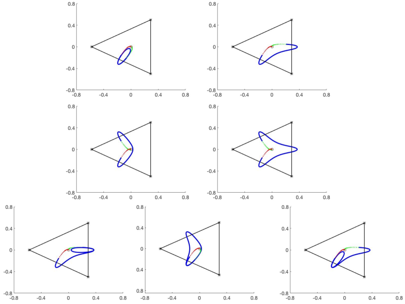
For example, the first 42 homoclinic connecting orbits (up to symmetry) at in the triple Copenhagen problem are classified in Table 5. These results are obtained by integrating initial local stable/unstable manifolds for time units subject to the speed constraint, . Our method finds all of the connections satisfying these constraints. The classification is in terms of the connection time, the order of appearance, and a geometric description in terms of words and letters.
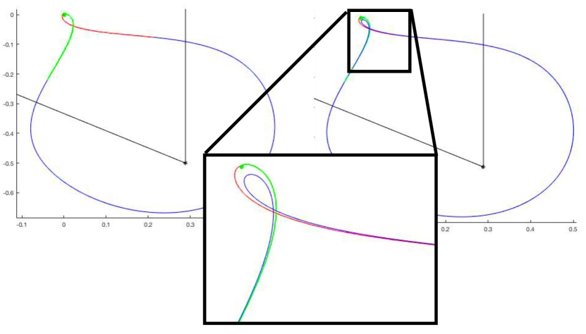
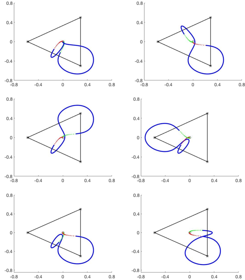
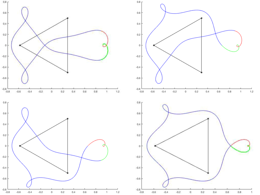
We give the names and to the shortest two connections at . These orbits are illustrated in Figure 10, and have connection times approximately 1.717 and 2.331 respectively. Rotating either of these by degrees gives another connecting orbit with exactly the same shape and connection time. We refer to these rotations as and . These six shortest connections – and their symmetric counterparts – organize the rest of the homoclinic behavior seen at as we now describe.
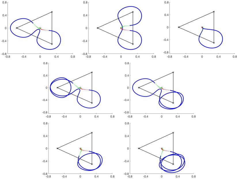
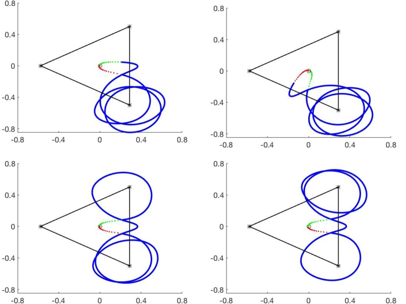
We associate the third shortest connection with the word because the orbit moves off the unstable manifold appearing to follow , passes near the equilibrium at , and makes another excursion following before returning to the stable manifold. Similarly we associate to the th longest connecting orbit the word , as this orbit moves off the unstable manifold and appears to follow , making two loops around the second primary before returning to the stable manifold. Heuristically speaking, , and their symmetric counterparts comprise a system of “homoclinic channels” or simple allowable motions and other homoclinic orbits seem to follow in their wake.
Table 6 records analogous information for the first 23 connections found at in the triple Copenhagen problem. In this case there are six basic letters . Words are formed for these letters just as discussed above. Applying degree rotations produces connections with the same shapes and connection times at and respectively. We stress that this description of the connecting orbits in terms of words and letters, while intuitively appealing, is based on qualitative observations and is subordinate to the rigid quantitative classification of the orbits by connection time.
Remark 12
Several comments about the results reported in Tables 5 and 6 are in order.
-
•
Additional symmetries: Some of the orbits, for example the 27th and 28th shortest orbits at and the 21st and 22nd shortest orbits at have reported the same connection times to three decimal places. In fact the connection times agree to within numerical errors. This is because the equal mass problem has reversible symmetries that we are not exploiting in our computations. Rather these serve as a check on the numerics.
-
•
Connection time versus ordering: While the connection times reported in these tables depend on the choice of local stable/unstable manifold, it should be remarked that, as long as the parameterization method is used to represent the local manifolds as discussed in Section 3, the ordering of the connections does not change. It is easy to check that the boundary of the parameterized manifolds are inflowing/outflowing and that the manifolds intersect only at the equilibrium solution. Moreover, since the eigenvalues are complex conjugate, the local parameterizations are unique up to the choice of a single eigenvector scale factor. By choosing the unit disk as the domain of the parameterization, the scaling the only free parameter in the problem. Decreasing the scaling by a factor of is equivalent to flowing the boundary by the same time . So: rescaling the eigenvectors changes all the times of flight by exactly the same amount, hence does not reorder them.
-
•
Qualitative classification: the decomposition of the connecting orbits into words is performed “by eye” in the present work. That is, we simply inspect the connections and describe what we see. We now sketch a method which could be used to formalize our qualitative description, and note that the idea is computationally feasible. Recall that if is a simple closed rectifiable curve in the plane (with counter clockwise orientation), and is a point not on , then the number of times that winds around is counted by the integral
So, observe for example that the curve winds once around the libration point , while and each wind once, respectively around and . Similarly the curve winds once around the second primary, while and wind once each around the third and first primaries. Then for a homoclinic orbit at define the integer vector , where for and both for . (Here are the coordinates of the th primary). Then counts the contribution of to while counts the contribution of and so on. This description amounts to an Abelianization of the previous notion of words/letters, as the winding vector looses track of the order of the letters in the word. (It is often the case that mechanical calculation of topological data is facilitated by passing to an Abeleanization). This notion is extended to the homoclinic orbits at in a similar way, see Figure 18.
-
•
Blue skies: the main theorem of Henrard in MR0365628 , already mentioned in the introduction, gives that there is a family of periodic orbits accumulating to each of the homoclinic orbits found by our procedure. In some cases we can venture a guess as which families of periodic orbits accumulate to which homoclinic. For example Figure 17 illustrates the orbit and along with the planar Lyapunov families attached to the inner libration points . The results suggest that the planar families may accumulate at to these homoclinics. Similarly, comparing the orbits and in the bottom left and right frames of Figure 18 with the planar Lyapunov families at illustrated in the left frame of Figure 3 suggests that these may be the families of periodic orbits attached to these homoclinics. The orbits , and , as well as the orbits and must be the limits of families of periodic orbits winding around the primary bodies. Making a systematic study of the periodic families associated with the homoclinic orbits discussed here would make a nice topic for a future study.
Remark 13 (Some related work on asymptotic orbits)
There are interesting similarities between some of the orbits discussed above, and some asymptotic orbits already discovered in papadakisPO_likeUs . The interested reader might for example compare the homoclinic orbit on the bottom right frame of our Figure 20 with the heteroclinic termination orbit illustrated in Figure 5 of papadakisPO_likeUs . (To make such a comparison one has to “flip” Figure 5 of papadakisPO_likeUs degrees about the -axis as the two papers use different normalizations of the four body problem. Also, their is our ). In that study the heteroclinic is discovered by numerical continuation of the author’s family of periodic orbits: a family of orbits with winding number one about all three of the primary masses. We note that our homoclinic of Figure 20 is similar, but that the degree rotational symmetry broken. We conjecture that there are three families of periodic orbits bifurcating from the family after a symmetry breaking, and that these families terminate on the homoclinic of Figure 20 (bottom right) and its rotation by degree counterparts.
Similarly, the heteroclinic orbit illustrated in Figure 4 of papadakisPO_likeUs – which is the termination of the author’s family – is related the pair of homoclinic orbits illustrated in our Figure 18. To see this, imagine an orbit obtained by combining our with the orbit , that is our rotated by degrees so that it is based at . The resulting union of curves has the same shape as the heteroclinic illustrated in Figure 4 of papadakisPO_likeUs . This suggests that the families of periodic orbits which terminate at our could emerge from the planar Lyapunov families after symmetry breaking.
In general we note that the homoclinic orbits tend to have less symmetry than the heteroclinic, so that studying the periodic orbits terminating at the homoclinics is a good way to obtain asymmetric periodic orbits – even in the symmetric versions of the problem. We also note that changing the mass parameters will tend to destroy heteroclinic connections, as the libration points will move into distinct energy levels. Homoclinic orbits on the other hand persist under generic Hamiltonian perturbations of the vector field. In particular they persist after a small change in the mass ratios, facilitating numerical continuation as discussed below.
5.4 Numerical continuation of ensembles of connections
The fact that the homoclinic connecting orbits are formulated as solutions of boundary value problems makes parameter continuation natural. We give only an outline of our continuation algorithm, as numerical continuation of homoclinic orbits for Hamiltonian systems is described in great detail in the literature. References are discussed in the introduction.
Begin with an ensemble of connecting orbits for a libration point at the mass parameters (initially we have ).
-
•
We choose a new parameter set , . Then we compute , and apply a first order predictor corrector to find the libration point at the new parameter values. We numerically compute the eigenvalues and eigenvectors of the new libration point, and if it remains a saddle-focus (i.e. if there has been no bifurcation) we proceed.
-
•
We recompute the local invariant manifolds at the new parameter set. A good strategy is to compute the coefficients to order by recursively solving the homological equations. Initially we take the eigenvector scaling from the previous step and rescale if needed. For the higher order coefficients we use the coefficients from the previous step. This gives as an initial guess for the Newton or pseudo-Newton method which usually converges very fast.
-
•
The new local parameterizations provide the boundary conditions for the multiple shooting scheme for the homoclinic orbits. We take the connecting orbits from the previous step as the initial guesses for the Newton method at the current mass parameters. If necessary we can apply a first order predictor corrector, but this is often unnecessary, due to the fact that the boundary value problem formulated with the high order parameterizations of the local manifold is very well conditioned. Note that in a given continuation step, the same local parameterizations serve as the boundary conditions for the entire ensemble of connecting orbits. This justifies the cost of computing high order representations of the manifolds.
-
•
Once we have applied Newton to all the connections in the ensemble we are ready to take a new step. If Newton fails to converge for any of the connecting orbits we have to decide if we throw the orbit away, or if we recompute with smaller .
We also remark that the atlas is not recomputed at the new mass parameter set. That is, we continue only the connecting orbits – the intersections of the stable unstable manifolds – not the manifolds themselves. Continuation of ensembles of connections is much cheaper than recomputing the atlas each time we change parameters.
Results of several numerical continuations are illustrated in Figures 21 and 22. As we change the masses we break the rotational symmetry of the Triple Copenhagen problem and the symmetric counterparts resolve into distinct connection, no longer obtainable by rotations of a single representative. During the numerical continuation we sometimes encounter bifurcations of the connecting orbits themselves, which involve no bifurcation of the underlying equilibrium. Figure 23 illustrates a common scenario where a family of homoclinic orbits undergoes a doubling bifurcation. These bifurcations seem very common and we have not made a systematic effort to track them. This would make an interesting topic for a future study.
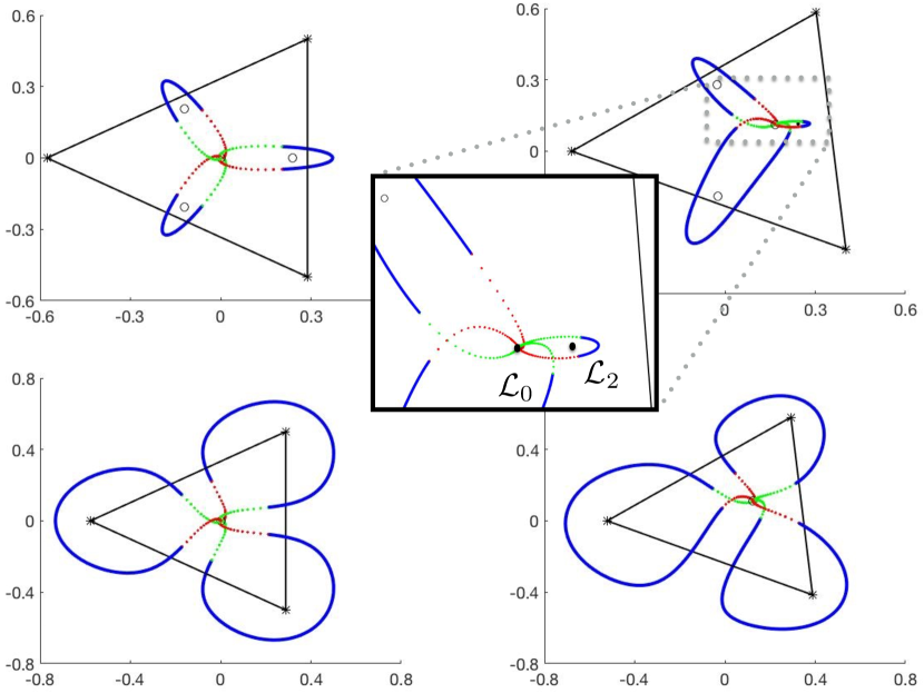
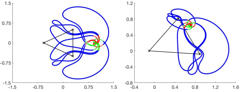
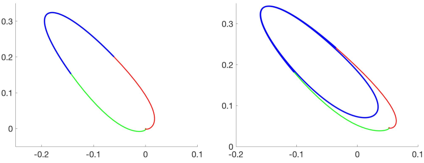
6 Conclusions
In this work we implemented a numerical method for computing an atlas for the stable/unstable manifold attached to a libration point in the CRFBP. We consider saddle-focus equilibria, as in this case topological theorems give rich dynamical structure near a transverse homoclinic. We then developed algorithms for searching or “mining” the atlas for approximate connections. After an approximate connection is found we sharpen it using a Newton scheme for an appropriate boundary value problem. The procedure is completely automated, and locates all the homoclinic orbits up to a specified integration time. (To make the calculations less stiff we ignore orbits passing too close to the primaries). The resulting collection of homoclinic orbits is ordered by connection time. A different choice of local parameterization may yield different connection times, but the ordering of these connections is universal. This last comment requires that the local stable/unstable manifolds are computed using the parameterizaiton method.
Our method locates dozens of distinct homoclinic connections and we consider their qualitative properties in addition to their connection times. The geometry of the homoclinic orbit set is organized by the several shortest connections, in the sense that they form a system of channels that other connections appear to follow. We decompose the motions of the longer connections into words built from these simple letters, and discuss briefly how this decomposition could be calculated in an automated way using the formulation of the winding number as a complex line integral.
Finally, we continue some of the orbits found in the equal mass case to other non-symmetric mass values using a predictor corrector scheme for the boundary value problem. Rather than recomputing the entire atlas the continuation scheme only recomputes the initial parameterization at the new masses, and this can be done via a Newton scheme.
We remark that it would be easy to intersect that atlas data computed here with any desired surface of section. We have not used sections in the present work because (a) we wanted to find all the connections up to a certain integration time and a given section may find some orbits and not others, and (b) projecting to a section may not preserve the ordering of the homoclinics by connection time. Moreover, while the present project focuses on the CRFBP – a two degree of freedom Hamiltonian system – the scheme described here could be extended to higher dimensional systems were sections are four or more dimensional and hence less useful for visualization purposes. In such a situation, for example the spatial CRFBP, it is desirable to have an automated procedure.
Other interesting topics of future research would be to combine our methods with more sophisticated continuation and branch following algorithms. It would also be nice to return to the ideas of Strömgren, and examine the “tubes” of periodic orbits attached to each of our homoclinic connections. These periodic families would themselves undergo bifurcations which one could try to follow numerically.
Another improvement to our method would be to remove the speed constraints on our manifold computations. This could be done by regularizing binary collisions. The idea would be that whenever a chart gets too close to a primary, then instead of subdividing we would change to the regularized coordinates where computations are less stiff. This idea of using such regularizations to improve numerics goes back at least to the work of Thiele. This would also provide a natural way for computing collision orbits between and each of the primaries. A topic we have avoided via our imposed speed constraints. A modern implementation combined with our approach to computing atlases would be valuable, and is the subject of ongoing work.
If such advancements let us compute larger and more complete atlases, a very interesting question is to see if other “fundamental” connecting orbits appear. For example at all the connections we find shadow two basic orbits , and their symmetric counterparts. Is this true of all the connections? Or is this simply an artifact of the fact that we only consider connections whose velocity is never too large? Will performing longer searches yield more fundamental letters for the alphabets at ?
Of course with more computing power one could perform the atlas computations at more values of the mass parameters, say for a mesh of ten or twenty different points in the simplex . This would provide a more complete picture of the global orbit structure. Such a project would greatly benefit form a cluster computing implementation exploiting the data independence of the computations at different parameter sets, and indeed the independence of different portions of the atlas at a given parameter set. Numerical continuation could then be applied to “fill in the gaps” between the mesh points.
Acknowledgements.
The authors would like to sincerely thank two anonymous referees who carefully read the submitted version of the manuscript. Their suggestions greatly improved the final version. The second author was partially supported by NSF grant DMS-1813501. Both authors were partially supported by NSF grant DMS-1700154 and by the Alfred P. Sloan Foundation grant G-2016-7320.Appendix A Rotational symmetry for the equal mass case
Let and . Define the linear map, , by
Note that acts as a rotation by in the and coordinate planes independently. Now, suppose that is a trajectory for , then is also a trajectory for . Moreover, if for , then , where is the permutation given by .
Proof
Let and suppose is the trajectory through satisfying . By definition, , and we note that will parameterize a trajectory for if and only if is tangent to for all . Thus, it clearly suffices to prove that holds for any on .
With this in mind, define the planar rotation by
Recall that for the symmetric mass case, we have equal masses given by . Set , then the primaries are located at given by
and note that . Moreover, are vertices of an equilateral triangle and a direct computation shows that acts as a cyclic permutation on the primary bodies in configuration space given by the cycle . Recalling that , it follows from this symmetry that for we have
| (17) |
Now, we recall that in the symmetric case, the CRFBP vector field is given by
which we write in scalar coordinates as . Similarly, write and we note that . Now, we check that holds for each . For , we have the direction computation
Now, for we first compute each expression
After canceling like terms in each expression, we are left to prove the following equality
| (18) |
Applying the result from (17) to the left side we have
so that for each , the numerator for is given by . Now, we compute the numerators for on the right hand side as
We conclude that the numerators for each are equal, and therefore, the equality in (18) holds which proves that . The proofs for the cases are computationally similar to the corresponding proofs for which concludes the proof that , or equivalently, is a trajectory for .
To prove the second claim, fix and suppose as implying that . Let , and note that is an equilibrium solution for implying that . Noting that is a unitary operator, it follows that as well. Moreover, is a dynamical conjugacy implying that in configuration space we have
Taken together it follows that is again an equilibrium solution for . Thus, acts as a permutation on equilibria. A direct computation shows that where is the permutation given by . The preceding argument applies equally well to the unstable manifold of each equilibrium with which completes the proof of the second claim.
Appendix B Power series manipulation, automatic differentiation, and the radial gradient
Our local invariant manifold computations are based on formal power series manipulations. The main technical challenge is to compute with an arbitrary power series and the vector field for the CRFBP. As usual in gravitational body problems, the nonlinearity contains terms raised to the minus three halves power.
Consider two formal power series given by
where for all . The collection of all formal power series forms a complex vector space, so that for any we have that
The collection becomes an algebra when endowed with the Cauchy product
| (19) |
We evaluate elementary functions of formal power series using a technique called automatic differentiation by many authors. Suppose for example we are given a formal series
with . We seek the formal series coefficients of the function
Our approach follows the discussion given by Alex Haro in mamotreto . Consider the first order partial differential operator
which is referred to as the radial gradient of . Evaluating on the level of formal power series leads to
Observe that
Multiplying both sides of the equation by we obtain
| (20) |
Here the fractional power is replaced by operations involving only differentiation and multiplication. This is the virtue of the radial gradient in automatic differentiation schemes. Plugging the power series expansions into Equation (20) leads to
and taking Cauchy products gives
Match like powers to get
or
for . Here
The appears to remind us that terms of order are extracted from the sum. Isolating gives
| (21) |
for . Note that by hypothesis, so that the coefficients are formally well defined to all orders. Using the recursion given in Equation (21) we can compute the formal series coefficients for for the cost of a Cauchy product. This allows us to compute power series representations for the nonlinear terms in and in the CRFBP. Another approach which converts the CRFB field to a higher dimensional polynomial filed in discussed in shaneAndJay .
Appendix C Conflict of interest statement
The authors of this manuscript certify that they have no affiliations with or involvement in any organization or entity with any financial interest (such as honoraria; educational grants, participation in speaker’s bureaus, membership, employment, consultancies, stock ownership, or other equity interest, and expert testimony or patent-licensing arrangements), or non-financial interest (such as personal or professional relationships, affiliations, knowledge or beliefs) in the subject matter or materials discussed in this manuscript.
References
- (1) G. H. Darwin. Periodic Orbits. Acta Math., 21(1):99–242, 1897.
- (2) E. Strömgren. Connaissance actuelle des orbites dans le probleme des trois corps. Bull. Astron., 9:87–130, 1934.
- (3) F.R. Moulton, D. Buchanan, T Buck, F.L. Griffin, W.R. Longley, and W.D. MacMillan. Periodic Orbits. Number Publication No. 161. Carnegie Institution of Washington, 1920.
- (4) V. Szebehely and P. Nacozy. A class of e. strömgren’s direct orbits in the restricted problem. The Astronomical Journal, 77(2):184–190, 1967.
- (5) V. Szebehely and Flandern T.V. A family of retegrade orbits around the triangular equilibrium points. The Astronomical Journal, 72(3):373–379, 1967.
- (6) V. Szebehely. Theory of Orbits. Academic Press Inc., 1967.
- (7) Jacques Henrard. Proof of a conjecture of E. Strömgren. Celestial Mech., 7:449–457, 1973.
- (8) Ralph H. Abraham. Chaostrophes, intermittency, and noise. In Chaos, fractals, and dynamics (Guelph, Ont., 1981/1983), volume 98 of Lecture Notes in Pure and Appl. Math., pages 3–22. Dekker, New York, 1985.
- (9) Leonid Pavlovich Shilnikov, Andrey L. Shilnikov, and Dmitry V. Turaev. Showcase of blue sky catastrophes. Internat. J. Bifur. Chaos Appl. Sci. Engrg., 24(8):1440003, 10, 2014.
- (10) Robert L. Devaney. Blue sky catastrophes in reversible and Hamiltonian systems. Indiana Univ. Math. J., 26(2):247–263, 1977.
- (11) Robert L. Devaney. Homoclinic orbits in Hamiltonian systems. J. Differential Equations, 21(2):431–438, 1976.
- (12) L. M. Lerman. Dynamical phenomena near a saddle-focus homoclinic connection in a Hamiltonian system. Journal of Statistical Physics, 101(1/2):357–372, 2000.
- (13) L. M. Lerman. Complex dynamics and bifurcations in a Hamiltonian system having a transversal homoclinic orbit to a saddle focus. Chaos, 1(2):174–180, 1991.
- (14) L. P. Shilńikov. On the question of the structure of an extended neighborhood of a structurally stable state of equilibrium of saddle-focus type. Mat. Sb. (N.S.), 81 (123):92–103, 1970.
- (15) L.P. Shilńikov. A contribution to the problem of the structure of an extended neighborhood of a rough equilibrium state of saddle-focus type. Mathematics of the USSR-Sbornik, 10(1):91, 1970.
- (16) L. P. Shilńikov. Existence of a countable set of periodic motions in a four-dimensional space in an extended neighborhood of a saddle-focus. Dokl. Akad. Nauk SSSR, 172:54–57, 1967.
- (17) P. Pedersen. Librationspunkte im restringierten vierkörperproblem. Dan. Mat. Fys. Medd., 21(6), 1944.
- (18) P. Pedersen. Stabilitätsuntersuchungen im restringierten vierkörperproblem. Dan. Mat. Fys. Medd., 26(16), 1952.
- (19) Carlos Simó. Relative equilibrium solutions in the four-body problem. Celestial Mech., 18(2):165–184, 1978.
- (20) A. N. Baltagiannis and K. E. Papadakis. Equilibrium points and their stability in the restricted four-body problem. Internat. J. Bifur. Chaos Appl. Sci. Engrg., 21(8):2179–2193, 2011.
- (21) Martha Álvarez-Ramí rez and Claudio Vidal. Dynamical aspects of an equilateral restricted four-body problem. Math. Probl. Eng., pages Art. ID 181360, 23, 2009.
- (22) Eduardo S. G. Leandro. On the central configurations of the planar restricted four-body problem. J. Differential Equations, 226(1):323–351, 2006.
- (23) Jean F. Barros and Eduardo S. G. Leandro. The set of degenerate central configurations in the planar restricted four-body problem. SIAM J. Math. Anal., 43(2):634–661, 2011.
- (24) Jean F. Barros and Eduardo S. G. Leandro. Bifurcations and enumeration of classes of relative equilibria in the planar restricted four-body problem. SIAM J. Math. Anal., 46(2):1185–1203, 2014.
- (25) K. E. Papadakis. Families of asymmetric periodic solutions in the restricted four-body problem. Astrophys. Space Sci., 361(12):Paper No. 377, 15, 2016.
- (26) K. E. Papadakis. Families of three-dimensional periodic solutions in the circular restricted four-body problem. Astrophys. Space Sci., 361(4):Paper No. 129, 14, 2016.
- (27) Jaime Burgos-García and Joaquín Delgado. Periodic orbits in the restricted four–body problem with two equal masses. Astrophysics and Space Sciencs, 345(2):247–263, 2013.
- (28) Jaime Burgos-García and Abimael Bengochea. Horseshoe orbits in the restricted four-body problem. Astrophys. Space Sci., 362(11):Paper No. 212, 14, 2017.
- (29) Jaime Burgos-García , J.P. Lessard, and J. D. Mireles James. Spatial periodic orbits in the equaliteral circular restricted four body problem: computer assisted proofs of existence. (Submitted), 2018.
- (30) Jaime Burgos-García . Families of periodic orbits in the planar Hill’s four-body problem. Astrophys. Space Sci., 361(11):Paper No. 353, 21, 2016.
- (31) Jaime Burgos-García and Marian Gidea. Hill’s approximation in a restricted four-body problem. Celestial Mech. Dynam. Astronom., 122(2):117–141, 2015.
- (32) Martha Alvarez-Ramírez, Joaquín Delgado, and Claudio Vidal. Global regularization of a restricted four-body problem. Internat. J. Bifur. Chaos Appl. Sci. Engrg., 24(7):1450092, 15, 2014.
- (33) Marian Gidea and Melissa Burgos. Chaotic transfers in three- and four-body systems. Phys. A, 328(3-4):360–366, 2003.
- (34) M. Alvarez-Ramírez and E. Barrabés. Transport orbits in an equilateral restricted four-body problem. Celestial Mech. Dynam. Astronom., 121(2):191–210, 2015.
- (35) Xuhua Cheng and Zhikun She. Study on chaotic behavior of the restricted four-body problem with an equilateral triangle configuration. Internat. J. Bifur. Chaos Appl. Sci. Engrg., 27(2):1750026, 12, 2017.
- (36) Zhikun She and Xuhua Cheng. The existence of a Smale horseshoe in a planar circular restricted four-body problem. Celestial Mech. Dynam. Astronom., 118(2):115–127, 2014.
- (37) Zhikun She, Xuhua Cheng, and Cuiping Li. The existence of transversal homoclinic orbits in a planar circular restricted four-body problem. Celestial Mech. Dynam. Astronom., 115(3):299–309, 2013.
- (38) Martha Alvarez-Ramírez, A. García, J.F. Palacián, and P. Yanguas. Oscillatory motions in restricted n-body problems. Journal of Differential Equations, 265:779–803, 2018.
- (39) Jaime Burgos-García and Joaquín Delgado. On the “blue sky catastrophe” termination in the restricted four-body problem. Celestial Mech. Dynam. Astronom., 117(2):113–136, 2013.
- (40) Shane Kepley and J. D. Mireles James. Chaotic motions in the restricted four body problem via Devaney’s saddle-focus homoclinic tangle theorem. to appear in Journal of Differential Equations, 2018.
- (41) X. Cabré, E. Fontich, and R. de la Llave. The parameterization method for invariant manifolds. I. Manifolds associated to non-resonant subspaces. Indiana Univ. Math. J., 52(2):283–328, 2003.
- (42) X. Cabré, E. Fontich, and R. de la Llave. The parameterization method for invariant manifolds. II. Regularity with respect to parameters. Indiana Univ. Math. J., 52(2):329–360, 2003.
- (43) X. Cabré, E. Fontich, and R. de la Llave. The parameterization method for invariant manifolds. III. Overview and applications. J. Differential Equations, 218(2):444–515, 2005.
- (44) W. Kalies, S. Kepley, and J.D. Mireles James. Analytic continuation of local (un)stable manifolds with rigorous computer assisted error bounds. SIAM Journal on Applied Dynamical Systems, 17(1):157–202, 2018.
- (45) Eusebius J. Doedel and Mark J. Friedman. Numerical computation of heteroclinic orbits. J. Comput. Appl. Math., 26(1-2):155–170, 1989. Continuation techniques and bifurcation problems.
- (46) E. J. Doedel, M. J. Friedman, and B. I. Kunin. Successive continuation for locating connecting orbits. Numer. Algorithms, 14(1-3):103–124, 1997. Dynamical numerical analysis (Atlanta, GA, 1995).
- (47) Wang Sang Koon, Martin W. Lo, Jerrold E. Marsden, and Shane D. Ross. Heteroclinic connections between periodic orbits and resonance transitions in celestial mechanics. Chaos, 10(2): 427–469, 2000.
- (48) E. Canalias, and J.J. Masdemont. Homoclinic and heteroclinic transfer trajectories between planar Lyapunov orbits in the sun-earth and earth-moon systems. Discrete and Continuous Dynamical Systems. Series A, 14(2): 261–279, 2006.
- (49) E. Barrabés, J.M. Mondelo, and M. Ollé. Numerical continuation of families of homoclinic connections of periodic orbits in the RTBP. Nonlinearity, 22(12):2901–2918, 2009.
- (50) A. R. Champneys, Yu. A. Kuznetsov, and B. Sandstede. A numerical toolbox for homoclinic bifurcation analysis. Internat. J. Bifur. Chaos Appl. Sci. Engrg., 6(5):867–887, 1996.
- (51) Àlex Haro, Marta Canadell, Jordi-Lluís Figueras, Alejandro Luque, and Josep-Maria Mondelo. The parameterization method for invariant manifolds, volume 195 of Applied Mathematical Sciences. Springer, [Cham], 2016. From rigorous results to effective computations.
- (52) Jean-Philippe Lessard, J. D. Mireles James, and Julian Ransford. Automatic differentiation for Fourier series and the radii polynomial approach. Physica D. 334(1):174 - 186, 2016.
- (53) Eugene Rabe. Determination and survey of periodic Trojan orbits in the restricted problem of three bodies. Astronom. J., 66:500–513, 1961.
- (54) Rafael de la Llave and J. D. Mireles James. Parameterization of invariant manifolds by reducibility for volume preserving and symplectic maps. Discrete Contin. Dyn. Syst., 32(12):4321–4360, 2012.
- (55) J. B. Van den Berg, J. D. Mireles James, and Christian Reinhardt. Computing (un)stable manifolds with validated error bounds: non-resonant and resonant spectra. Journal of Nonlinear Science, 26:1055–1095, 2016.
- (56) S.M. Rump. INTLAB - INTerval LABoratory. In Tibor Csendes, editor, Developments in Reliable Computing, pages 77–104. Kluwer Academic Publishers, Dordrecht, 1999. http://www.ti3.tu-harburg.de/rump/.
- (57) A. N. Baltagiannis and K. E. Papadakis. Families of periodic orbits in the restricted four-body problem. Astrophysics and Space Sciencs, 336:357–367, 2011.