Remarks on the Casimir Self-Entropy of a Spherical Electromagnetic $\delta$-Function Shell

Abstract

Recently the Casimir self-entropy of an electromagnetic $\delta$-function shell was considered by two different groups, with apparently discordant conclusions, although both had concluded that a region of negative entropy existed for sufficiently weak coupling. We had found that the entropy contained an infrared divergence, which we argued should be discarded on physical grounds. On the contrary, Bordag and Kirsten recently found a completely finite self-entropy, although they, in fact, have to remove an infrared divergence. Apart from this, the high- and low-temperature results for finite coupling agree precisely for the transverse electric mode, but there are significant discrepancies in the transverse magnetic mode. We resolve those discrepancies here. In particular, it is shown that coupling-independent terms do not occur in a consistent regulated calculation, they likely being an artefact of the omission of pole terms. The results of our previous analysis, especially, the existence of a negative entropy region for sufficiently weak coupling, are therefore confirmed. Finally, we offer some analogous remarks concerning the Casimir entropy of a thin electromagnetic sheet, where the total entropy is always positive. In that case, the origin of the analogous discrepancy can be explicitly isolated.

I Introduction

The entropy due to electromagnetic field fluctuations, or Casimir entropy, of a perfectly conducting spherical shell (of radius $a$) was computed many years ago by Balian and Duplantier bd , who found the following low and high temperature behaviors for the free energy,

$$\Delta F_{\infty}\sim-\frac{(\pi a)^{3}}{15}T^{4},\quad aT\ll 1;\qquad F_{\infty}\sim-\frac{T}{4}(\ln aT+0.7686),\quad aT\gg 1.$$ (1)

Here the subscript is a reminder that the conductivity of the sphere is considered infinite, and the $\Delta$ means this is the correction to the zero-temperature Casimir energy of the sphere, first calculated by Boyer boyer . Only recently was this calculation generalized to a spherical shell with a finite electromagnetic coupling, a so-called electromagnetic $\delta$-function shell, or a spherical plasma shell Milton:2017ghh ; bordagandkirsten . The former is described by the background permittivity

$$\bm{\varepsilon}(\mathbf{r})-\bm{1}=\lambda(\bm{1}-\mathbf{rr})\delta(r-a),$$ (2)

which describes a sphere of radius $a$ centered at the origin. The anisotropy is required by Maxwell’s equations, as detailed in Refs. Parashar:2012it ; Parashar:2017sgo . We further assume that the medium is dispersive, with a plasma-model like dispersion relation, $\lambda=\lambda_{0}/(\zeta^{2}a)$, with $\lambda_{0}$ a dimensionless constant, in terms of the imaginary frequency $\zeta$. This model is approximately realistic, and the transverse electric (TE) mode in this model coincides with the analogous scalar field model. It also coincides with the plasma-shell model considered by Bordag and Kirsten in Ref. bordagandkirsten . To translate parameters in the model in that reference to ours, we note that their $R$ is the same as our $a$, and $\Omega R$ coincides with $\lambda_{0}$. When $\lambda_{0}\to\infty$ we recover the perfectly conducting spherical shell.

In this note we will make a detailed comparison between the results found in Refs. bordagandkirsten and Milton:2017ghh . We will see that the finite coupling results found at low and high temperature agree for the TE mode, which is by far easier to treat. There are some discrepancies in the transverse magnetic (TM) contributions to the entropy. We see no sign of the coupling-independent high-temperature TM term in the free energy found in Ref. bordagandkirsten ; this arises because the heat-kernel approach incorrectly incorporates $\lambda^{0}$ terms, apparently due to the omission of a pole term in the frequency integration. However, the high-temperature term linear in the coupling coincides with our findings, and results from the exact treatment of the $O(\lambda_{0})$ terms. At low temperature, Ref. bordagandkirsten gives only the result for $\lambda_{0}\gg(aT)^{2}$, that is, for the temperature being the smallest scale in the problem; we show that their machinery yields our result for arbitrary values of $aT/\sqrt{\lambda_{0}}$. The low temperature behavior will be described in Sec. II, while the high-temperature limit will be discussed in Sec. III. Finally, we note that we disagree with their procedure of subtracting the leading high temperature terms in the free energy; doing so would violate the strong-coupling limit given in Eq. (1), which we reproduce but was initially unmentioned, except at zero temperature, in Ref. bordagandkirsten . Indeed, in the revised version of bordagandkirsten they perform a different subtraction for the perfectly conducting sphere, so a smooth limit is not possible.

Details of the new calculations for the sphere are relegated to Appendices A and B. In Appendix C we discuss the entropy of a flat electromagnetic sheet which we considered earlier in Ref. Li:2016oce , and has now been revisited by Bordag bordagfs . Again, there is disagreement about the coupling-independent term, this time in the TE mode, as well as about what is to be subtracted. This changes the physical conclusions, in that we find the total entropy to be always positive; and the total entropy for a perfectly conducting sheet is zero. Mathematically one can see essential agreement of all the terms found in the two approaches. In particular, in Appendix D we show how our result is reproduced using the Abel-Plana formula, which yields a expression very similar to that seen in Bordag’s paper bordagfs , differing only by a crucial extra term. The latter is the origin of the discrepant coupling-independent term. In Appendix E we identify the exact origin of this discrepancy: In the passage from the real-frequency expression for the entropy to that obtained from the phase-shift expression used in Ref. bordagfs , a pole contribution was omitted. (Such seems to have been done in Ref. bordagfs , as we also show in Appendix E.) We believe a similar omission occurs in the sphere calculation, although because of its greater complexity, it is less transparent to detect.

II Low Temperature Regime of the Free Energy

The leading low temperature correction given by Ref. bordagandkirsten is in our notation (disregarding the subtraction of the high-temperature contribution, to which we return later)

$$F_{T\to 0}=-\frac{\pi^{3}}{15}\frac{6+\lambda_{0}}{3+\lambda_{0}}a^{3}T^{4}=\frac{(\pi a)^{3}T^{4}}{15}\left(\frac{1}{1+3/\lambda_{0}}-2\right),$$ (3)

where the first term is the TE contribution and the second the TM. The TE term in the free energy is precisely that given in Ref. Milton:2017ghh , see Eq. (6.3) there. The second term is the TM free energy found there as well, see Eq. (6.13), if $aT\ll\sqrt{\lambda_{0}}$, that is, if the dimensionless temperature $aT$ is the smallest quantity in the problem. However, if this is not the case, there are corrections parameterized by $\xi=\frac{\alpha}{\sqrt{2\lambda_{0}/3}}$, where we’ve introduced the abbreviation $\alpha=2\pi aT$. We obtained closed form expressions for the TM free energy for low temperatures as a function of $\xi$, see Eq. (17). For small $\xi$ the result coincides with that contained in Eq. (3),

$$\xi\ll 1:\quad F^{\rm TM}\sim-\frac{2}{15}(\pi a)^{3}T^{4},$$ (4)

which is Eq. (6.22) of Ref. Milton:2017ghh , while for large $\xi$ the result coincides with the high-temperature limit of the exact result for the TM free energy in $O(\lambda_{0})$:

$$\xi\gg 1:\quad F^{\rm TM}\sim\frac{2}{9}\lambda_{0}\pi aT^{2},$$ (5)

as stated in Eq. (6.23) of Ref. Milton:2017ghh . This implies negative entropy occurs for small coupling and temperature. (The TE contribution is always negative.)

These results may be easily reproduced using the methods of Ref. bordagandkirsten . The details are given in Appendix A.

III High Temperature Regime of the Free Energy

Here there seems more discrepancy between the two approaches, but again the results coincide for the TE mode. We both have for large $aT$ (fixed $\lambda_{0}$) that [Eq. (7.17) of Ref. Milton:2017ghh ]

$$aT\gg 1:\quad F^{\rm TE}\sim\frac{\lambda_{0}\pi aT^{2}}{6},$$ (6)

which results from the exact free energy in the lowest-order in $\lambda_{0}$. On the other hand, Ref. bordagandkirsten gives

$$aT\gg 1:\quad F^{\rm TM}\sim-2\zeta(3)a^{2}T^{3}+\frac{\lambda_{0}\pi aT^{2}}{18}.$$ (7)

The second term is the same as the high temperature limit again of the $O(\lambda_{0})$ term given in Eq. (7.30) of Ref. Milton:2017ghh , but we saw no evidence of the first term in Eq. (7), which seems counterintuitive because it persists even if the coupling goes to zero. But we did not examine the general high temperature result for fixed $\lambda_{0}$ in our earlier paper, but only in the strong coupling (perfectly conducting) limit. We remedy that deficiency now in Appendix B, and again only find the term of $O(\lambda_{0})$ in Eq. (7). This again implies negative entropy occurs even at high temperature for sufficiently small coupling. The reason for the discrepancy with the result of Ref. bordagandkirsten , which was calculated by a rather elaborate method in Ref. bordagandkushnutdinov , is that we used the exact uniform asymptotic expansion (UAE) for Euclidean frequencies together with the rapidly convergent Chowla-Selberg formula elizalde1 ; elizalde2 , so a term independent of $\lambda_{0}$ cannot occur in our calculation.

Indeed, we can recover a term of the same form as the first term in Eq. (7) by including, erroneously, a $k=0$ term in Eq. (24), with the leading asymptotic term given by Eq. (28). Evidently the approach used in Ref. bordagandkirsten does not correctly omit the $(\lambda_{0})^{0}$ contribution from the free energy. This is further elucidated in the flat sheet case in Appendices D and E; in the former, we show that the Abel-Plana formula, which recasts our Euclidean approach into real frequencies, yields our, not Bordag’s, result, and in the latter, we identify the pole term that transforms Bordag’s free energy into ours.

IV Discussion

Therefore, we have shown substantial agreement between the results of Refs. bordagandkirsten and Milton:2017ghh , for the free energy of a $\delta$-function sphere. The agreement is perfect for the TE mode. The TM mode is more subtle. There, at low temperature, the calculations agree if the temperature (in units of the inverse radius of the sphere) is the smallest quantity, but we point out that there are interesting corrections if $\lambda_{0}/(aT)^{2}$ is small, resulting in a sign change in the entropy. At high temperature, again we exactly agree with the term linear in the coupling, but we see no evidence of a term in the free energy, independent of $\lambda_{0}$, proportional to $T^{3}$. We believe this term is an artefact of the method employed by Bordag et al. In the case of a flat sheet, the Abel-Plana formula, which we would expect to yield results equivalent to the heat-kernel approach used in Ref. bordagfs , in fact resums the free energy into a form which does yield our weak-coupling expansion Li:2016oce . This is discussed in Appendix D. We identify the extra pole term that resolves this discrepancy in Appendix E; we expect a similar resolution in the sphere case, but the analysis is more involved there. Refs. Milton:2017ghh ; Li:2016oce use temporal and spatial point-splitting, permitting weak- and strong-coupling expansions. Working with Euclidean frequencies removes ambiguities in the branch lines of the square roots.

Ref. bordagandkirsten does not make any comparison of their results with ours. This is surprising, but they justify this by remarking that our procedure results in some divergent terms. However, at the end of the calculation there was only an infrared-sensitive term

$$F^{\rm TM}_{\rm IR}=T\ln\frac{\mu}{T}.$$ (8)

This we argued should be removed as an irrelevant contact term, since it does not refer to the sphere parameters, and indeed precisely such a term can be seen to be removed implicitly in the calculation given in Ref. bordagandkirsten , as one can verify by examining the arguments in Ref. bordagandkushnutdinov .

Finally, we must address the subtraction procedure advocated in Ref. bordagandkirsten . The argument given there is that the two leading high-temperature terms seen in Eq. (7) should be subtracted because they do not possess a classical limit. But doing so would seem to challenge the self-consistency of the theory, and would result in changing the well-established perfectly conducting sphere limit, which is indeed acknowledged in the revised version of their paper bordagandkirsten . Subtracting their leading, coupling-independent, term from the free energy further introduces an explicitly negative entropy term for weak coupling.

Both calculations discussed in this note find that there is a negative entropy region, which seems in contradiction with the physical, thermodynamical meaning of entropy. However, as Ref. bordagandkirsten seems to acknowledge, neither of us are accounting for the complete physical system. The background, in our case, the $\delta$-function potential, and in their case, the plasma shell, are established by forces other than those arising from the electromagnetic fluctuating fields whose effects we are calculating. A thorough investigation including the complete physical system would yield a positive total entropy.

As we were completing the first version of this note, Bordag posted a new paper bordagfs which discusses the electromagnetic thin sheet, which we had considered earlier in Ref. Li:2016oce . As we have already mentioned, in Appendices C, D we again show essential agreement between our two approaches, although Bordag again finds a spurious $\lambda_{0}$-independent term in now the TE component of the free energy, which discrepancy is resolved in Appendix E, and advocates subtractions for which we see no necessity.

Appendix A The low temperature limit of the TM free energy

In this appendix we sketch how the methods of Ref. bordagandkirsten yield exactly the same result for $F^{\rm TM}$ in the low temperature limit as found in Ref. Milton:2017ghh . Bordag and Kirsten compute the free energy from the phase shifts, defined here by

$$\delta_{l}^{\rm TM}=-\frac{\pi}{2}+\arctan\frac{1-\frac{\lambda_{0}}{x}\tilde{\jmath}_{l}^{\prime}(x)\tilde{y}_{l}^{\prime}(x)}{\frac{\lambda_{0}}{x}[\tilde{\jmath}_{l}^{\prime}(x)]^{2}},\quad x=\omega a,$$ (9)

where the Riccati-Bessel functions are defined in terms of the usual spherical Bessel functions by $\tilde{\jmath}_{l}(x)=xj_{l}(x)$, $\tilde{y}_{l}(x)=xy_{l}(x)$. For small temperature, all that is relevant is the leading low frequency behavior, which arises only for $l=1$ (larger values of $l$ give higher powers of $T$):

$$\delta_{1}^{\rm TM}\sim-\pi+\frac{2}{3}x^{3}.$$ (10)

From this limit the result (4) follows. However, if $x$ and $\lambda_{0}$ are comparable, there are corrections:

$$\delta^{\rm TM}_{1}=-\pi+\frac{2}{3}x^{3}\sum_{k=0}^{\infty}\left(\frac{3}{2}\frac{x^{2}}{\lambda_{0}}\right)^{k}.$$ (11)

In the scheme given in Ref. bordagandkirsten the temperature correction to the free energy is given by the formula

$$\Delta_{T}F=T\int_{0}^{\infty}\frac{d\omega}{\pi}\ln\left(1-e^{-\omega/T}\right)\frac{d}{d\omega}\delta(\omega),\quad\delta=\sum_{l=1}^{\infty}(2l+1)\delta_{l}.$$ (12)

This result may be readily derived from the real-frequency version of Eq. (18). Inserting the expansion (11) into this, we find

$$\Delta_{T}F=-\frac{2}{\pi}T\sum_{k=0}^{\infty}(2k+3)\left(\frac{3}{2\lambda_{0}}\right)^{k}(aT)^{3+2k}\Gamma(2k+3)\zeta(2k+4),$$ (13)

and then if we use the Euler representation of the gamma function we have

$$\Delta_{T}F=-2\frac{a^{3}T^{4}}{\pi}\int_{0}^{\infty}dt\,t^{3}e^{-t}f\left(\frac{\xi t}{2\pi}\right),\quad\xi=\frac{2\pi aT}{\sqrt{2\lambda_{0}/3}},$$ (14)

where

$$f(y)=\sum_{k=0}^{\infty}y^{2k}\zeta(2k+4)=\frac{3-\pi^{2}y^{2}-3\pi y\cot\pi y}{6y^{4}}.$$ (15)

This expression actually does not exist because of poles in the cotangent; the radius of convergence of the series is 1. Such poles are characteristic of real-frequency formulations. However, we may find a unique analytic continuation by making, for example, a $\pi/4$ rotation in the integration variable, $t\to t(1+i)$,

$$\Delta_{T}F^{\rm TM}=-\left(\frac{2\lambda_{0}}{3}\right)^{2}\frac{1}{\pi a}\frac{\xi^{4}}{8\pi^{4}}(1+i)^{4}\int_{0}^{\infty}dt\,t^{3}e^{-t(1+i)}f\left(\frac{\xi t}{2\pi}(1+i)\right),$$ (16)

which is absolutely convergent. This is an alternative “closed-form” to that shown in Ref. Milton:2017ghh , and gives the limits shown above in Eqs. (4), (5). It coincides with the form given in our paper [Eq. (6.24)] for all $\xi$ [$(\pi a)^{-1}$ was inadvertently omitted there],

$$\Delta_{T}F^{\rm TM}=\left(\frac{2\lambda_{0}}{3}\right)^{2}\frac{1}{\pi a}\left[\frac{\xi^{2}}{12}-\ln\xi-\Re\psi\left(1+\frac{i}{\xi}\right)\right],$$ (17)

as seen in Fig. 1, which is equivalent to Fig. 3 in Ref. Milton:2017ghh . This further shows that the TM entropy (the negative slope of the free energy with respect to $T$) is positive for strong coupling (small $\xi$), and negative for weak coupling (large $\xi$), with the transition occurring near $\xi_{0}=1.75\dots$.

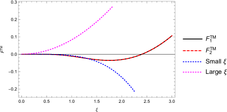
Figure 1: The free energy computed from either Eq. (16) or Eq. (17), which coincide, compared with the leading low $\xi$ approximation (lower dotted, blue) and with the leading large $\xi$ approximation (upper dotted, magenta). The latter approaches the exact result closely for larger $\xi$ than shown in the figure.

Appendix B The high temperature limit of the TM free energy

The general expression for the TM component of the free energy for a electromagnetic $\delta$-function shell is (Eq. (2.10) of Ref. Milton:2017ghh )

$$F^{\rm TM}=\frac{T}{2}\sum_{n=-\infty}^{\infty}\sum_{l=1}^{\infty}(2l+1)\ln\left(1-\frac{\lambda_{0}}{x}e_{l}^{\prime}(x)s_{l}^{\prime}(x)\right),\quad x=n\alpha,\quad\alpha=2\pi aT,$$ (18)

where we see the appearance of the modified Riccati-Bessel functions,

$$s_{l}(x)=\sqrt{\frac{\pi x}{2}}I_{l+1/2}(x),\quad e_{l}(x)=\sqrt{\frac{2x}{\pi}}K_{l+1/2}(x).$$ (19)

To get the high-temperature behavior, it is convenient to first use the uniform asymptotic expansion (UAE) for the Bessel functions, which leads to the expansion of the logarithm appearing here:

$$\ln\left(1-\frac{\lambda_{0}}{x}e_{l}^{\prime}(x)s_{l}^{\prime}(x)\right)\sim\sum_{k=1}^{\infty}\frac{a^{(k)}_{\rm TM}(z)}{(2\nu)^{k}},\quad x=\nu z,\quad\nu=l+1/2,\quad t=(1+z^{2})^{-1/2}.$$ (20)

The first four of these coefficients are given in Eq. (7.26) of Ref. Milton:2017ghh . The leading term is that with the highest power of $\lambda_{0}$ in each coefficient, which amounts to retaining only the leading order uniform asymptotic expansion of the Bessel functions within the logarithm. Therefore we approximate the increasingly elaborate structure of the expansion coefficients by

$$a_{\rm TM}^{(k)}\sim(-1)^{k+1}\frac{1}{k}\left(\frac{\lambda_{0}}{z^{2}t}\right)^{k}.$$ (21)

This then leads to the approximate form (the prime designates 1/2 weight for $n=0$)

$$F^{\rm TM}\sim T\sum_{k=1}^{\infty}(-1)^{k+1}\frac{1}{k}\sum_{n=0}^{\infty}{}^{\prime}\sum_{l=1}^{\infty}2\nu\left(\frac{\lambda_{0}}{2\nu z^{2}}\right)^{k}(1+z^{2})^{k/2},\quad z=n\alpha/\nu$$ (22)

This is actually incorrect for $n=0$, where we should use the small argument expansion of the Bessel functions, as explained in Ref. Milton:2017ghh . The $n=0$ term requires an infrared regulator, and is a bit subtle, but however it is precisely defined, it can only contribute an $O(T)$ contribution, smaller than the leading terms we are seeking.

So to extract the leading high-temperature contributions to the free energy, we consider

$$F^{\rm TM}_{n>0}\sim T\sum_{k=1}^{\infty}\sum_{n=0}^{\infty}\sum_{l=0}^{\infty}(2l+3)\frac{(-1)^{k+1}}{k}\left(\frac{\lambda_{0}}{2}\right)^{k}\frac{[(l+3/2)^{2}+\alpha^{2}(n+1)^{2}]^{k/2}}{[\alpha^{2}(n+1)^{2}]^{k}}.$$ (23)

Here we have shifted the $n$ and $l$ variables down by 1 to put the sum in standard form. This expression does not actually exist; we will define it by analytically continuing the exponent in the numerator to $s-1<-1/2$, and then at the end continuing back to $s=1+k/2$. We can take care of the factor of $2l+3$ by differentiating with respect to $b$, a variable to be set to 3/2 at the end. In this way our approximation reads

$$F^{\rm TM}_{n>0}\sim T\sum_{k=1}^{\infty}\frac{(-1)^{k+1}}{k}\left(\frac{\lambda_{0}}{2}\right)^{k}\frac{1}{s}\frac{\partial}{\partial b}Z,$$ (24)

where

$$Z=\sum_{n,l=0}^{\infty}\frac{[(l+b)^{2}+\alpha^{2}d(n+1)^{2}]^{s}}{[(n+1)^{2}\alpha^{2}]^{k}}.$$ (25)

We have introduced yet another parameter $d$, to be set to 1 at the end, so that by differentiating with respect to $d$ we can get rid of the denominator:

$$\left(\frac{\partial}{\partial d}\right)^{k}Z=\frac{\Gamma(s+1)}{\Gamma(s+1-k)}E_{2}(k-s;1,d\alpha^{2};b,1).$$ (26)

In this expression we have followed the notation of Elizalde elizalde1 ; elizalde2 . The high temperature behavior is captured by the generalized Chowla-Selberg formula given there [see Eq. (7.3) of Ref. Milton:2017ghh ):

$$E_{2}(k-s;1,d\alpha^{2};b,1)\sim(d\alpha^{2})^{s-k}\zeta(0,b)\zeta(2k-2s),$$ (27)

with higher terms being down by powers of $\alpha^{-2}$. Then we can integrate up the derivatives seen in Eq. (26), but there are $k$ integration constants:

$$Z\sim d^{s}\alpha^{2s-2k}\zeta(0,b)\zeta(2k-2s)+\sum_{j=0}^{k-1}A_{j}d^{j},$$ (28)

where we can now set $d=1$ and $s=k/2+1$. The integration constants $A_{j}$ can be readily computed by evaluating $Z$ and its derivatives at $d=0$. However, these constants are innocuous for extracting the leading behavior: For a given power of $\lambda_{0}$ in the free energy, the largest term in $\alpha$ comes from the $A_{k-1}$ term, which goes like $\alpha^{-2}$, subdominant compared to the leading terms. Therefore we disregard those terms, do the $b$ derivative by noticing that

$$\frac{\partial}{\partial b}\zeta(0,b)\bigg{|}_{b=3/2}=-1,$$ (29)

and write ($aT\to\infty$)

$$F^{\rm TM}\sim-T\alpha^{2}\left[\frac{\lambda_{0}}{2\alpha}\frac{2}{3}\zeta(-1)-\frac{1}{2}\left(\frac{\lambda_{0}}{2\alpha}\right)^{2}\frac{1}{2}\zeta(0)+\frac{1}{3}\left(\frac{\lambda_{0}}{2\alpha}\right)^{3}\frac{2}{5}\zeta(1)+\sum_{k=4}^{\infty}\frac{(-1)^{k+1}}{k}\left(\frac{\lambda_{0}}{2\alpha}\right)^{k}\frac{1}{1+k/2}\zeta(k-2)\right].$$ (30)

The sum turns out to be of order $(\lambda_{0}/2\alpha)^{3}$; but that and the third divergent term are temperature independent. The second term here is of order $T$, but that must be supplemented by the $n=0$ term which we deferred above. Thus, all we can extract is the leading term for high temperature,

$$F^{\rm TM}\sim\frac{\lambda_{0}\pi aT^{2}}{18},\quad aT\gg 1,\lambda_{0},$$ (31)

which coincides with the second term in Eq. (7), and which, as anticipated, agrees with the high temperature limit of the exact $O(\lambda_{0})$ solution. No sign appears of the first term in Eq. (7), which is coupling-independent. The reason for the discrepancy with that of the procedure used in Ref. bordagandkushnutdinov is that our regulated expressions for the free energy vanish in the absence of interactions, so there can be no contribution at $\lambda_{0}=0$. It appears, as demonstrated in Appendix E for the analogous flat sheet problem, that in translating the free energy expression into the phase-shift formulation used in Refs. bordagandkirsten and bordagfs a pole term has been omitted, whose inclusion would cancel the offending term. The unregulated heat-kernel technique, unlike the Abel-Plana formula, discussed in Appendix D, inserts spurious coupling-independent terms. Further evidence for the appropriateness of our approach lies in the strong-coupling (perfect conductor) limit, where there is a term of just such a form in both the TE and TM modes, occurring with equal magnitudes and opposite signs, so they cancel in the total free energy. (This was seen also in Refs. bkmm ; geyer .) Here, the term appears only in the TM mode. Finally we note that in our procedure, detailed in Ref. Milton:2017ghh , where no such term appears, we do recover the Balian and Duplantier] result (1) for the perfect-conductor, high-temperature limit. No smooth limit is possible in the scheme advocated in Ref. bordagandkirsten .

Appendix C Thin electromagnetic sheet

In Ref. Li:2016oce we exactly solved for the Casimir entropy of a flat electromagnetic $\delta$-function sheet, described by the permittivity $\bm{\varepsilon}(\mathbf{r})-\bm{1}=\mbox{diag}(\lambda,\lambda,0)\delta(z)$. We showed that the TE entropy is always negative, while the TM entropy is positive, and always larger than the magnitude of the former. The total entropy tends to zero in the limit $\lambda\to\infty$, that is, for a perfectly conducting sheet. Results were precisely defined using temporal and spatial point-splitting regulators.

Closed form results were obtained for the entropy for a “plasma model,” where the dispersion was incorporated by writing $\lambda=\lambda_{0}/\zeta^{2}$, where $\lambda_{0}$ is a constant, and $\zeta$ is the imaginary frequency. (For the flat sheet, $\lambda_{0}$ has the dimension of (length)^-1. The explicit forms for the TE and TM entropies per unit area are given by (4.13) and (4.25) of Ref. Li:2016oce . We will content ourselves here by writing the limits:

$$T\gg\lambda_{0}:\quad S^{\rm TE} \sim -\frac{\lambda_{0}}{12}T+O(T^{0}),$$ (32a)

$$T\ll\lambda_{0}:\quad S^{\rm TE} \sim -\frac{3\zeta(3)}{4\pi}T^{2}+O(T^{3}),$$ (32b)

and

$$T\gg\lambda_{0}:\quad S^{\rm TM} \sim \frac{120\zeta(5)}{\pi\lambda_{0}^{2}}T^{4}+\frac{3\zeta(3)}{2\pi}T^{2}-\frac{\lambda_{0}}{36}T+O(T^{0}),$$ (33a)

$$T\ll\lambda_{0}:\quad S^{\rm TM} \sim \frac{3\zeta(3)}{4\pi}T^{2}+O(T^{3}).$$ (33b)

Notice that these results mean that the total entropy vanishes in the perfect conducting limit.

Ref. bordagfs seems to obtain somewhat different limits. For high temperature, Bordag gives (with his $\Omega_{0}=\lambda_{0}/2$ and $\omega_{0}=0$) for the TE contributions,

$$T\gg\lambda_{0}:\quad S^{\rm TE}_{B}\sim\frac{3\zeta(3)}{4\pi}T^{2}-\frac{\lambda_{0}}{12}T,$$ (34)

so although the second term coincides with Eq. (32a), the first term was not seen by us. (The corresponding heat kernel coefficients were first worked out in Ref. Bordag:2005qv .) Again, this is presumably because our regulated expressions allow for a weak-coupling expansion. Indeed, were we to start the sum in Eq. (4.11) in Ref. Li:2016oce at $n=-1$ ($n=0$ is already explicitly included), we would obtain (taking the limit $n\to-1$) exactly the first term in Eq. (34). Again, this is clearly incorrect. Once more, because he subtracted both of these leading terms from the entropy, his subtracted TE entropy per unit area has a linear term at low temperature:

$$T\ll\lambda_{0}:\quad S^{\rm TE}_{B,\rm{sub}}\sim\frac{\lambda_{0}}{12}T,$$ (35)

the term shown in Eq. (32b) being of higher order.

For TM Bordag recognizes the first two terms in the high-temperature limit (33a) as the TM surface plasmon contributions ($\omega_{0}=0$), which he again subtracts, leaving precisely the third term there:

$$T\gg\lambda_{0}:\quad S^{\rm TM}_{B,{\rm sub1}}\sim-\frac{\lambda_{0}}{36}T,$$ (36)

but he subtracts this term away as well, leaving a low-temperature entropy per unit area exactly one-third of that for TE in Eq. (35):

$$T\ll\lambda_{0}:\quad S^{\rm TM}_{B,\rm{sub2}}=\frac{\lambda_{0}}{36}T,$$ (37)

because again the correction from Eq. (33b) is higher order. Note, that with Bordag’s prescription, the perfect conductor limit does not exist.

So the technical results of both paper coincide, as further shown in Appendix D. We disagree only the inclusion of spurious coupling-independent terms, and on the necessity of subtracting terms because they do not seem to reproduce known results. The following two Appendices help resolve the issue of the spurious terms.

Appendix D Abel-Plana formula

For simplicity, we consider here the TE mode of the free energy per area for the thin sheet, which is given by the spatially regulated formula (Eq. (4.1) of Ref. Li:2016oce )

$$F^{\rm TE}=\frac{T}{2\pi}\sum_{m=0}^{\infty}{}^{\prime}\int_{0}^{\infty}dk\,kJ_{0}(k\delta)\ln\left(1+\frac{\lambda_{0}}{2\kappa_{m}}\right),\quad\kappa_{m}=\sqrt{k^{2}+\zeta_{m}^{2}},$$ (38)

where the prime means the $m=0$ term is counted with half weight. The Abel-Plana formula allows us to turn the sum into an integral:

$$\sum_{m=0}^{\infty}{}^{\prime}f(m)=\int_{0}^{\infty}dt\,f(t)+i\int_{0}^{\infty}dt\frac{1}{e^{2\pi t}-1}[f(it)-f(-it)].$$ (39)

Using the first term here in the formula for the free energy (38) gives a term independent of temperature, which we disregard. For the second term we integrate by parts

$$\Delta F^{\rm TE}=\frac{T}{(2\pi)^{2}}\int_{0}^{\infty}dt\ln(1-e^{-2\pi t})[f^{\prime}(it)+f^{\prime}(-it)],$$ (40)

where

$$f(t)=\int_{0}^{\infty}dk\,kJ_{0}(k\delta)\ln\left(1+\frac{\lambda_{0}}{2\sqrt{k^{2}+(2\pi tT)^{2}}}\right).$$ (41)

The derivative of $f$ does not require the regulator:

$$f^{\prime}(t)=(2\pi T)^{2}t\ln\left(1+\frac{\lambda_{0}}{4\pi tT}\right).$$ (42)

and then with $\tilde{\omega}=2\pi t$, we have

$$f^{\prime}(it)+f^{\prime}(-it)=-4\pi T^{2}\tilde{\omega}\arctan\frac{\lambda_{0}}{2\tilde{\omega}T}.$$ (43)

In this way we obtain a result slightly different from what Bordag gives:

$$\Delta F^{\rm TE}=-\frac{T^{3}}{2\pi^{2}}\int_{0}^{\infty}d\tilde{\omega}\,\tilde{\omega}\ln\left(1-e^{-\tilde{\omega}}\right)\arctan\frac{\lambda_{0}}{2\tilde{\omega}T},$$ (44)

while Ref. bordagfs has the same formula with the arctangent replaced by $-\arctan\frac{2\tilde{\omega}T}{\lambda_{0}}=\arctan\frac{\lambda_{0}}{2\tilde{\omega}T}-\frac{\pi}{2}$.

If we expand the arctangent for large argument, we obtain the nearly the same leading high-temperature result that Bordag does:

$$\frac{T}{\lambda_{0}}\gg 1:\quad\Delta F\sim\frac{\lambda_{0}}{24}T^{2}-\frac{\lambda_{0}^{2}}{24}T\left(1-2\ln\frac{\lambda_{0}}{2T}\right),$$ (45)

which is consistent with Eq. (34), apart from the first term there. The two terms here agree with those found in Eq. (4.14b) of Ref. Li:2016oce , and, as shown there, the full series is convergent. In the opposite limit, that of low temperature or strong coupling, we obtain from Eq. (44) the asymptotic series

$$\frac{\lambda_{0}}{T}\gg 1:\quad\Delta F^{\rm TE}=-\frac{\zeta(3)}{4\pi}T^{3}-\frac{T^{3}}{2\pi^{2}}\sum_{n=0}^{\infty}(-1)^{n}\frac{\Gamma(2n+4)\zeta(2n+4)}{(2n+1)(2n+3)}\left(\frac{2T}{\lambda_{0}}\right)^{2n+1},$$ (46)

which coincides with our expansion (4.14a) of Ref. Li:2016oce . In general, we conclude that the difference between the two forms of the entropy is

$$S^{\rm TE}=S^{\rm TE}_{\rm B}-\frac{3\zeta(3)}{4\pi}T^{2}.$$ (47)

This suggests that that the properly regulated theory is that discussed in Ref. Li:2016oce , so the coupling-independent term is not present. This is demonstrated in the following Appendix.

Appendix E Resolution of Discrepancy

We now carefully rederive the starting point in Ref. bordagfs starting from the real-frequency form for the free energy ($\beta=1/T$), which follows directly from the familiar $\operatorname{Tr}\ln$ formula $F=-\frac{1}{2}\operatorname{Tr}\ln\bm{\Gamma}\bm{\Gamma}_{0}^{-1}$ in terms of the free and full Green’s dyadics $\bm{\Gamma}_{0}$ and $\bm{\Gamma}$. For the transverse electric contribution to the free energy this amounts to

$$\Delta F^{\rm TE} = \frac{1}{2\pi^{2}}\Im\int_{0}^{\infty}d\omega\frac{1}{e^{\beta\omega}-1}\int_{0}^{\infty}dk\,k\ln\left(1+\frac{\lambda_{0}}{2\sqrt{k^{2}-\omega^{2}}}\right)$$ (48)

$$= -\frac{\lambda_{0}}{4\pi^{2}\beta}\Im\int_{0}^{\infty}dk\,k\int_{0}^{\infty}d\omega\,\omega\ln\left(1-e^{-\beta\omega}\right)\frac{1}{k^{2}-\omega^{2}}\frac{1}{\lambda_{0}/2+\sqrt{k^{2}-\omega^{2}}}.$$

(Formally, this can be derived from the Euclidean form (38) by the Abel-Plana formula.) In the second line, we have integrated by parts and omitted the boundary term because it is real. There are two singularities in the $\omega$ integration above, a pole and a branch point, both occurring at $\omega=k$. We choose the branch line to pass from $k$ to $\infty$. In the spirit of using the causal or Feynman propagator, our contour of integration must pass above all of these singularities. Let us change variables from $\omega$ to $\kappa=\sqrt{k^{2}-\omega^{2}}$, where $\kappa$ is real for $\omega<k$ and $\kappa=-ik_{z}$ for $\omega>k$, the sign of $i$ being dictated by the above contour requirement. We then write the free energy as

$$\Delta F=-\frac{\lambda_{0}}{4\pi^{2}\beta}\Im\int_{0}^{\infty}dk\,k\left\{\int_{0}^{k}\frac{d\kappa}{\kappa}\frac{\ln\left(1-e^{-\beta\sqrt{k^{2}-\kappa^{2}}}\right)}{\lambda_{0}/2+\kappa}-\int_{0}^{\infty}\frac{dk_{z}}{k_{z}}\frac{\ln\left(1-e^{-\beta\sqrt{k^{2}+k_{z}^{2}}}\right)}{\lambda_{0}/2-ik_{z}}\right\}.$$ (49)

We will initially disregard the pole at $\kappa=k_{z}=0.$ Then the first term in the above is purely real, so it is to be discarded, and the imaginary part of what is left is

$$\Delta_{1}F=\frac{\lambda_{0}T}{4\pi^{2}}\int_{0}^{\infty}dk\,k\int_{0}^{\infty}dk_{z}\frac{1}{k_{z}^{2}+(\lambda_{0}/2)^{2}}\ln\left(1-e^{-\beta\sqrt{k^{2}+k_{z}^{2}}}\right).$$ (50)

This is precisely the formula (10) given in Ref. bordagfs , with the derivative of the phase shift (or the density of states factor) given there by

$$\frac{d}{dp}\delta(p)=\frac{\Omega_{0}}{\Omega_{0}^{2}+p^{2}},$$ (51)

which coincides with Eq. (30) of Bordag’s paper (with the first $\omega_{0}$ in the denominator replaced by $\Omega_{0}$.) (Remember our translation of variables: here $\Omega_{0}\to\lambda_{0}/2$, $p\to k_{z}$, and $\omega_{0}=0$.) This then leads directly, upon introducing polar coordinates, to Bordag’s results for the free energy and entropy:

$$\Delta_{1}F=\frac{T}{2\pi^{2}}\int_{0}^{\infty}d\omega\,\omega\ln\left(1-e^{-\beta\omega}\right)\arctan\frac{2\omega}{\lambda_{0}}.$$ (52)

Let us now include the pole terms that we omitted following Eq. (49). This gives another contribution to the imaginary part:

$$\Delta_{2}F=-\frac{\frac{\pi}{2}}{2\pi^{2}\beta}\int_{0}^{\infty}dk\,k\ln\left(1-e^{-\beta k}\right).$$ (53)

Combining this with the $\Delta_{1}F$ contribution yields our result (44).

In fact, Bordag’s starting point bordagfs

$$\Delta F^{\rm TE}=\int_{0}^{\infty}\frac{dp}{\pi}\int\frac{(d\mathbf{k})}{(2\pi)^{2}}T\ln\left(1-e^{-\beta\omega}\right)\frac{d\delta(p)}{dp},$$ (54)

properly interpreted, also yields the same result. This is because

$$\frac{d\delta(p)}{dp}=\Re\frac{\Omega_{0}}{p(p-i\Omega_{0})}$$ (55)

is not exactly Eq. (51) because $p$ contains an implicit branch line, with branch point at $p=0$. Thus

$$\Delta F^{\rm TE}=-T\Im\int_{0}^{\infty}\frac{dp}{\pi}\int\frac{dk\,k}{2\pi}\ln\left(1-e^{-\beta\omega}\right)\left(\frac{1}{p}-\frac{1}{p-i\Omega_{0}}\right).$$ (56)

The second term is Bordag’s result (50) and (52), while the first, evaluated by integrating over a quarter circle around the pole at $p=0$ in the positive sense, yields precisely our correction (53). (The sense of the contour is most easily seen starting from Eq. (48).)

The discrepancy is thus resolved. We presume a similar extra term occurs in the more complicated spherical calculation.

References

- (1) R. Balian, and B. Duplantier, “Electromagnetic waves near perfect conductors. 2. Casimir effect,” Ann. Phys. (N.Y.) 112, 165 (1978). doi:10.1016/0003-4916(78)90083-0
- (2) T. H. Boyer, “Quantum electromagnetic zero point energy of a conducting spherical shell and the Casimir model for a charged particle,” Phys. Rev. 174, 1764 (1968). doi:10.1103/PhysRev.174.1764
- (3) K. A. Milton, P. Kalauni, P. Parashar and Y. Li, “Casimir self-entropy of a spherical electromagnetic -function shell,” Phys. Rev. D 96, 085007 (2017) doi:10.1103/PhysRevD.96.085007 [arXiv:1707.09840 [hep-th]].
- (4) M. Bordag and K. Kirsten, “On the entropy of a spherical plasma shell,” arXiv:1805.11241.
- (5) P. Parashar, K. A. Milton, K. V. Shajesh and M. Schaden, “Electromagnetic semitransparent -function plate: Casimir interaction energy between parallel infinitesimally thin plates,” Phys. Rev. D 86, 085021 (2012) doi:10.1103/PhysRevD.86.085021 [arXiv:1206.0275 [hep-th]].
- (6) P. Parashar, K. A. Milton, K. V. Shajesh and I. Brevik, “Electromagnetic -function sphere,” Phys. Rev. D 96, 085010 (2017) doi:10.1103/PhysRevD.96.085010 [arXiv:1708.01222 [hep-th]].
- (7) Y. Li, K. A. Milton, P. Kalauni and P. Parashar, “Casimir self-entropy of an electromagnetic thin sheet,” Phys. Rev. D 94, 085010 (2016) doi:10.1103/PhysRevD.94.085010 [arXiv:1607.07900 [hep-th]].
- (8) M. Bordag, “Free energy and entropy for thin sheets,” Phys. Rev. D 98, 085010 (2018) [arXiv:1807.09691].
- (9) M. Bordag and N. Khusnutdinov, “Vacuum energy of a spherical plasma shell,” Phys. Rev. D 77, 085026 (2008).
- (10) E. Elizalde, “On the zeta-function regularization of a two-dimension series of Epstein-Hurwitz type,” J. Math. Phys. 31, 170–174 (1989).
- (11) E. Elizalde, “Ten physical applications of spectral zeta functions,” Lect. Notes Phys. Monogr. 35, 1 (1995). doi:10.1007/978-3-540-44757-3
- (12) M. Bordag, G. L. Klimchitskaya, U. Mohideen, and V. M. Mostepanenko, Advances in the Casimir Effect (Oxford, 2009).
- (13) B. Geyer, G. L. Klimchitskaya and V. M. Mostepanenko, “Thermal Casimir effect in ideal metal rectangular boxes,” Eur. Phys. J. C 57, 823 (2008) doi:10.1140/epjc/s10052-008-0698-z [arXiv:0808.3754 [quant-ph]].
- (14) M. Bordag, I. G. Pirozhenko and V. V. Nesterenko, “Spectral analysis of a flat plasma sheet model,” J. Phys. A 38, 11027 (2005) doi:10.1088/0305-4470/38/50/011 [hep-th/0508198].