Document Informed Neural Autoregressive Topic Models

Abstract

Context information around words helps in determining their actual meaning, for example “networks” used in contexts of artificial neural networks or biological neuron networks. Generative topic models infer topic-word distributions, taking no or only little context into account. Here, we extend a neural autoregressive topic model to exploit the full context information around words in a document in a language modeling fashion. This results in an improved performance in terms of generalization, interpretability and applicability. We apply our modeling approach to seven data sets from various domains and demonstrate that our approach consistently outperforms state-of-the-art generative topic models. With the learned representations, we show on an average a gain of $9.6$% ($0.57$ Vs $0.52$) in precision at retrieval fraction $0.02$ and $7.2$% ($0.582$ Vs $0.543$) in $F1$ for text categorization.

1 Introduction

Probabilistic topic models, such as LDA Blei et al. (2003), Replicated Softmax (RSM) Salakhutdinov and Hinton (2009) and Document Autoregressive Neural Distribution Estimator (DocNADE) Larochelle and Lauly (2012) are often used to extract topics from text collections and learn document representations to perform NLP tasks such as information retrieval (IR), document classification or summarization.

To motivate our task, assume that we conduct topic analysis on a collection of research papers from NIPS conference, where one of the popular terms is “networks”. However, without context information (nearby and/or distant words), its actual meaning is ambiguous since it can refer to such different concepts as artificial neural networks in computer science or biological neural networks in neuroscience or Computer/data networks in telecommunications. Given the context, one can determine the actual meaning of “networks”, for instance, “Extracting rules from artificial neural networks with distributed representations”, or “Spikes from the presynaptic neurons and postsynaptic neurons in small networks” or “Studies of neurons or networks under noise in artificial neural networks” or “Packet Routing in Dynamically Changing Networks”.

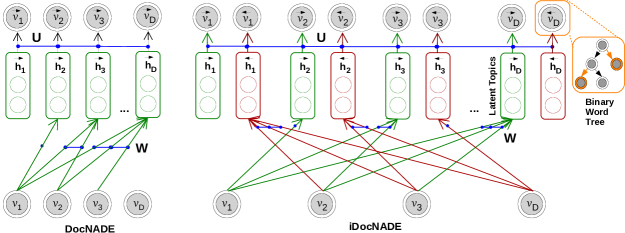
Figure 1: (Left): DocNADE (Right): iDocNADE (the proposed model). Blue colored lines signify the connections that share parameters. The observations (double circle) for each word $v_{i}$ are multinomial. Hidden vectors in green and red colors identify the forward and backward network layers, respectively. Symbols $\overrightarrow{v}_{i}$ and $\overleftarrow{v}_{i}$ represent the autoregressive conditionals $p(v_{i}|{\bf v}_{<i})$ and $p(v_{i}|{\bf v}_{>i})$, respectively. Connections between each $v_{i}$ and hidden units are shared, and each conditional $\overrightarrow{v}_{i}$ (or $\overleftarrow{v}_{i}$) is decomposed into a tree of binary logistic regressions, i.e. hierarchical softmax. Best viewed in color.

Generative topic models such as LDA or DocNADE infer topic-word distributions that can be used to estimate a document likelihood. While basic models such as LDA do not account for context information when inferring these distributions, more recent approaches such as DocNADE achieve amplified word and document likelihoods by accounting for words preceding a word of interest in a document. More specifically, DocNADE Larochelle and Lauly (2012); Zheng et al. (2016) (Figure 1, Left) is a probabilistic graphical model that learns topics over sequences of words, corresponding to a language model Manning and Schütze (1999); Bengio et al. (2003) that can be interpreted as a neural network with several parallel hidden layers. To predict the word $v_{i}$, each hidden layer ${\bf h}_{i}$ takes as input the sequence of preceding words ${\bf v}_{<i}$. However, it does not take into account the following words ${\bf v}_{>i}$ in the sequence. Inspired by bidirectional language models Mousa and Schuller (2017) and recurrent neural networks Elman (1990); Gupta et al. (2015a, 2016); Vu et al. (2016b, a), trained to predict a word (or label) depending on its full left and right contexts, we extend DocNADE and incorporate full contextual information (all words around ${v}_{i}$) at each hidden layer ${\bf h}_{i}$ when predicting the word ${v}_{i}$ in a language modeling fashion with neural topic modeling.

Contribution: (1) We propose an advancement in neural autoregressive topic model by incorporating full contextual information around words in a document to boost the likelihood of each word (and document). We demonstrate using 7 data sets from various domains that this enables learning better (informed) document representations in terms of generalization (perplexity), interpretability (topic coherence) and applicability (document retrieval and classification). We name the proposed topic model as Document Informed Neural Autoregressive Distribution Estimator (iDocNADE).

(2) With the learned representations, we show a gain of $9.6$% ($.57$ Vs $.52$) in precision at retrieval fraction 0.02 and $7.2$% ($.582$ Vs $.543$) in $F1$ for text categorization compared to the DocNADE model (on average over 6 data sets).

The code and pre-processed data is available at https://github.com/pgcool/iDocNADE.

2 Neural Autoregressive Topic Models

RSM Salakhutdinov and Hinton (2009); Gupta et al. (2018), a probabilistic undirected topic model is a generalization of the energy-based Restricted Boltzmann Machines RBM Hinton (2002); Gupta et al. (2015b, c), which can be used to model word counts. NADE Larochelle and Murray (2011) decomposes the joint distribution of observations into autoregressive conditional distributions, modeled using non-linear functions. Unlike for RBM and RSM, this leads to tractable gradients of the data negative log-likelihood but can only be used to model binary observations.

DocNADE (Figure 1, Left), a generative neural autoregressive topic model to account for word counts, is inspired by RSM and NADE. For a document ${\bf v}=[v_{1},...,v_{D}]$ of size $D$, it models the joint distribution $p({\bf v})$ of all words $v_{i}$, where $v_{i}\in\{1,...,K\}$ is the index of the $i$th word in the dictionary of vocabulary size $K$. This is achieved by decomposing it as a product of conditional distributions i.e. $p({\bf v})=\prod_{i=1}^{D}p(v_{i}|{\bf v}_{<i})$ and computing each autoregressive conditional $p(v_{i}|{\bf v}_{<i})$ via a feed-forward neural network for $i\in\{1,...D\}$,

$$\begin{split}\overrightarrow{\bf h}_{i}({\bf v}_{<i})&=g(D{\bf c}+\sum_{k<i}{\bf W}_{:,v_{k}})\end{split}$$

$$\begin{split}p(v_{i}=w|{\bf v}_{<i})&=\frac{\exp(b_{w}+{\bf U}_{w,:}\overrightarrow{\bf h}_{i}({\bf v}_{<i}))}{\sum_{w^{\prime}}\exp(b_{w^{\prime}}+{\bf U}_{w^{\prime},:}\overrightarrow{\bf h}_{i}({\bf v}_{<i}))}\end{split}$$

where ${\bf v}_{<i}\in\{v_{1},...,v_{i-1}\}$. $g(\cdot)$ is a non-linear activation function, ${\bf W}\in\mathbb{R}^{H\times K}$ and ${\bf U}\in\mathbb{R}^{K\times H}$ are weight matrices, ${\bf c}\in\mathbb{R}^{H}$ and ${\bf b}\in\mathbb{R}^{K}$ are bias parameter vectors. $H$ is the number of hidden units (topics). ${\bf W}_{:,<i}$ is a matrix made of the $i-1$ first columns of ${\bf W}$. Therefore, the log-likelihood $\mathcal{L}$ of a document v in DocNADE is computed as:

$$\mathcal{L}^{DocNADE}({\bf v})=\sum_{i=1}^{D}\log p(v_{i}|{\bf v}_{<i})$$ (1)

The probability of the word $v_{i}$ is computed using a position-dependent hidden layer $\overrightarrow{\bf h}_{i}({\bf v}_{<i})$ that learns a representation based on all previous words ${\bf v}_{<i}$; however it does not incorporate the following words ${\bf v}_{>i}$. Taken together, the likelihood $p(\bf v)$ of any document of arbitrary length can be computed. Note that, following RSM, we re-introduced the scaling factor $D$ in computing ${\bf h}_{i}$ to account for documents of different lengths, that is ignored in the original DocNADE formulation.

iDocNADE (Figure 1, Right), our proposed model accounts for the full context information (both previous ${\bf v}_{<i}$ and following ${\bf v}_{>i}$ words) around each word $v_{i}$ for a document ${\bf v}$. Therefore, the log-likelihood $\mathcal{L}^{iDocNADE}$ for a document $\bf v$ in iDocNADE is computed using forward and backward language models as:

$$\begin{split}\log p({\bf v})=\frac{1}{2}\sum_{i=1}^{D}\underbrace{\log p(v_{i}|{\bf v}_{<i})}_{\mbox{forward}}&+\underbrace{\log p(v_{i}|{\bf v}_{>i})}_{\mbox{backward}}\end{split}$$ (2)

$$\begin{split}\mathcal{L}^{iDocNADE}({\bf v})=\frac{1}{2}\Big{[}\overrightarrow{\mathcal{L}}({\bf v})&+\overleftarrow{\mathcal{L}}({\bf v})\Big{]}\end{split}$$ (3)

where $\mathcal{L}^{iDocNADE}$ is the mean of the forward ($\overrightarrow{\mathcal{L}}$) and backward ($\overleftarrow{\mathcal{L}}$) log-likelihoods. This is achieved in a bi-directional language modeling and feed-forward fashion by computing position dependent forward ($\overrightarrow{\bf h}_{i}$) and backward ($\overleftarrow{\bf h}_{i}$) hidden layers for each word $i$, as:

$$\begin{split}\overrightarrow{\bf h}_{i}({\bf v}_{<i})=g(D\overrightarrow{\bf c}+\sum_{k<i}{\bf W}_{:,v_{k}})\end{split}$$

$$\begin{split}\overleftarrow{\bf h}_{i}({\bf v}_{>i})=g(D\overleftarrow{\bf c}+\sum_{k>i}{\bf W}_{:,v_{k}})\end{split}$$

where $\overrightarrow{\bf c}\in\mathbb{R}^{H}$ and $\overleftarrow{\bf c}\in\mathbb{R}^{H}$ are bias parameters in forward and backward passes, respectively. $H$ is the number of hidden units (topics).

Two autoregressive conditionals are computed for each $i$th word using the forward and backward hidden vectors, as:

$$\begin{split}p(v_{i}=w|{\bf v}_{<i})=\frac{\exp(\overrightarrow{b}_{w}+{\bf U}_{w,:}\overrightarrow{\bf h}_{i}({\bf v}_{<i}))}{\sum_{w^{\prime}}\exp(\overrightarrow{b}_{w^{\prime}}+{\bf U}_{w^{\prime},:}\overrightarrow{\bf h}_{i}({\bf v}_{<i}))}\end{split}$$

$$\begin{split}p(v_{i}=w|{\bf v}_{>i})=\frac{\exp(\overleftarrow{b}_{w}+{\bf U}_{w,:}\overleftarrow{\bf h}_{i}({\bf v}_{>i}))}{\sum_{w^{\prime}}\exp(\overleftarrow{b}_{w^{\prime}}+{\bf U}_{w^{\prime},:}\overleftarrow{\bf h}_{i}({\bf v}_{>i}))}\end{split}$$

for $i\in[1,...,D]$ where $\overrightarrow{\bf b}\in\mathbb{R}^{K}$ and $\overleftarrow{\bf b}\in\mathbb{R}^{K}$ are biases in forward and backward passes, respectively. Observe, the parameters W and U are shared in the forward and backward networks.

Algorithm 1 Computation of $\log p({\bf v})$ using iDocNADE

1:Input: A training document vector v

2:Parameters: {$\overrightarrow{\bf b}$, $\overleftarrow{\bf b}$, $\overrightarrow{\bf c}$, $\overleftarrow{\bf c}$, W, U}

3:Output: $\log p({\bf v})$

4:$\overrightarrow{\bf a}\leftarrow\overrightarrow{\bf c}$

5:$\overleftarrow{\bf a}\leftarrow\overleftarrow{\bf c}+\sum_{i>1}{\bf W}_{:,v_{i}}$

6:$q({\bf v})=1$

7:for $i$ from $1$ to $D$ do

8:     $\overrightarrow{\bf h}_{i}\leftarrow g(\overrightarrow{\bf a})$

9:     $\overleftarrow{\bf h}_{i}\leftarrow g(\overleftarrow{\bf a})$

10:     $p(v_{i}|{\bf v}_{<i})=1$

11:     $p(v_{i}|{\bf v}_{>i})=1$

12:     for $m$ from $1$ to $|{\bf\pi}(v_{i})|$ do

13:         $p(v_{i}|{\bf v}_{<i})\leftarrow p(v_{i}|{\bf v}_{<i})p({\bf\pi}(v_{i})_{m}|{\bf v}_{<i})$

14:         $p(v_{i}|{\bf v}_{>i})\leftarrow p(v_{i}|{\bf v}_{>i})p({\bf\pi}(v_{i})_{m}|{\bf v}_{>i})$      

15:     $q({\bf v})\leftarrow q({\bf v})p(v_{i}|{\bf v}_{<i})p(v_{i}|{\bf v}_{>i})$

16:     $\overrightarrow{\bf a}\leftarrow\overrightarrow{\bf a}+{\bf W}_{:,v_{i}}$

17:     $\overleftarrow{\bf a}\leftarrow\overleftarrow{\bf a}-{\bf W}_{:,v_{i}}$

18:$\log p({\bf v})\leftarrow\frac{1}{2}\log q({\bf v})$

Algorithm 2 Computing gradients of $-\log p({\bf v})$ in iDocNADE

1:Input: A training document vector v

2:Parameters: {$\overrightarrow{\bf b}$, $\overleftarrow{\bf b}$, $\overrightarrow{\bf c}$, $\overleftarrow{\bf c}$, W, U}

3:Output: $\delta\overrightarrow{\bf b},\delta\overleftarrow{\bf b},\delta\overrightarrow{\bf c},\delta\overleftarrow{\bf c},\delta{\bf W},\delta{\bf U}$

4:$\overrightarrow{\bf a}\leftarrow 0$; $\overleftarrow{\bf a}\leftarrow 0$; $\overrightarrow{\bf c}\leftarrow 0$; $\overleftarrow{\bf c}\leftarrow 0$; $\overrightarrow{\bf b}\leftarrow 0$; $\overleftarrow{\bf b}\leftarrow 0$

5:for $i$ from $D$ to $1$ do

6:     $\delta\overrightarrow{\bf h}_{i}\leftarrow 0$

7:     $\delta\overleftarrow{\bf h}_{i}\leftarrow 0$

8:     for $m$ from $1$ to $|{\bf\pi}(v_{i})|$ do

9:         $\overrightarrow{b}_{l{(v_{i})_{m}}}\leftarrow\overrightarrow{b}_{l{(v_{i})_{m}}}+(p(\pi(v_{i})_{m}|{\bf v}_{<i})-\pi(v_{i})_{m})$

10:         $\overleftarrow{b}_{l{(v_{i})_{m}}}\leftarrow\overleftarrow{b}_{l{(v_{i})_{m}}}+(p(\pi(v_{i})_{m}|{\bf v}_{>i})-\pi(v_{i})_{m})$

11:         $\delta\overrightarrow{\bf h}_{i}\leftarrow\delta\overrightarrow{\bf h}_{i}+(p(\pi(v_{i})_{m}|{\bf v}_{<i})-\pi(v_{i})_{m}){\bf U}_{l(v_{i})m,:}$

12:         $\delta\overleftarrow{\bf h}_{i}\leftarrow\delta\overleftarrow{\bf h}_{i}+(p(\pi(v_{i})_{m}|{\bf v}_{>i})-\pi(v_{i})_{m}){\bf U}_{l(v_{i})m,:}$

13:         $\delta{\bf U}_{l(v_{i})_{m}}\leftarrow\delta{\bf U}_{l(v_{i})_{m}}+(p(\pi(v_{i})_{m}|{\bf v}_{<i})-\pi(v_{i})_{m})\overrightarrow{\bf h}_{i}^{T}+(p(\pi(v_{i})_{m}|{\bf v}_{>i})-\pi(v_{i})_{m})\overleftarrow{\bf h}_{i}^{T}$      

14:     $\delta\overrightarrow{\bf g}\leftarrow\overrightarrow{\bf h}_{i}\circ(1-\overrightarrow{\bf h}_{i})$ # for sigmoid activation

15:     $\delta\overleftarrow{\bf g}\leftarrow\overleftarrow{\bf h}_{i}\circ(1-\overleftarrow{\bf h}_{i})$ # for sigmoid activation

16:     $\delta\overrightarrow{\bf c}\leftarrow\delta\overrightarrow{\bf c}+\delta\overrightarrow{\bf h}_{i}\circ\delta\overrightarrow{\bf g}$

17:     $\delta\overleftarrow{\bf c}\leftarrow\delta\overleftarrow{\bf c}+\delta\overleftarrow{\bf h}_{i}\circ\delta\overleftarrow{\bf g}$

18:     $\delta{\bf W}_{:,v_{i}}\leftarrow\delta{\bf W}_{:,v_{i}}+\delta\overrightarrow{\bf a}+\delta\overleftarrow{\bf a}$

19:     $\delta\overrightarrow{\bf a}\leftarrow\delta\overrightarrow{\bf a}+\delta\overrightarrow{\bf h}_{i}\circ\delta\overrightarrow{\bf g}$

20:     $\delta\overleftarrow{\bf a}\leftarrow\delta\overleftarrow{\bf a}+\delta\overleftarrow{\bf h}_{i}\circ\delta\overleftarrow{\bf g}$

Learning: Similar to DocNADE, the autoregressive conditionals $p(v_{i}=w|{\bf v}_{<i})$ and $p(v_{i}=w|{\bf v}_{>i})$ in iDocNADE are computed by a neural network for each word $v_{i}$, allowing efficient learning of informed representations $\overrightarrow{\bf h}_{i}$ and $\overleftarrow{\bf h}_{i}$, as it consists simply of a linear transformation followed by a non-linearity. Observe that the weight $\bf W$ is the same across all conditionals and ties (blue colored lines) contextual observables by computing each $\overrightarrow{\bf h}_{i}$ or $\overleftarrow{\bf h}_{i}$.

Binary word tree to compute conditionals: The computations of each of the autoregressive conditionals $p(v_{i}=w|{\bf v}_{<i})$ and $p(v_{i}=w|{\bf v}_{>i})$ require time linear in $K$, which is expensive to compute for $i\in[1,2,...D]$. Following Larochelle and Lauly (2012), we decompose the computation of the conditionals to achieve a complexity logarithmic in $K$. All words in the documents are randomly assigned to a different leaf in a binary tree and the probability of a word is computed as the probability of reaching its associated leaf from the root. Each left/right transition probability is modeled using a binary logistic regressor with the hidden layer $\overrightarrow{\bf h}_{i}$ or $\overleftarrow{\bf h}_{i}$ as its input. In the binary tree, the probability of a given word is computed by multiplying each of the left/right transition probabilities along the tree path.

Algorithm 1 shows the computation of $\log p({\bf v})$ using the iDocNADE structure, where the autogressive conditionals (lines 10 and 11) for each word $v_{i}$ are obtained from the forward and backward networks and modeled into a binary word tree, where $\pi(v_{i})$ denotes the sequence of binary left/right choices at the internal nodes along the tree path and ${\bf l}(v_{i})$ the sequence of tree nodes on that tree path. For instance, $l(v_{i})_{1}$ will always be the root of the binary tree and $\pi(v_{i})_{1}$ will be 0 if the word leaf $v_{i}$ is in the left subtree or 1 otherwise. Therefore, each of the forward and backward conditionals are computed as:

$$\begin{split}p(v_{i}=w|{\bf v}_{<i})&=\prod_{m=1}^{|\pi(v_{i})|}p(\pi(v_{i})_{m}|{\bf v}_{<i})\end{split}$$

$$\begin{split}p(v_{i}=w|{\bf v}_{>i})&=\prod_{m=1}^{|\pi(v_{i})|}p(\pi(v_{i})_{m}|{\bf v}_{>i})\end{split}$$

$$\begin{split}p(\pi(v_{i})_{m}|{\bf v}_{<i})=&g(\overrightarrow{b}_{l{(v_{i})_{m}}}+{\bf U}_{l{(v_{i})_{m}},:}\overrightarrow{\bf h}({\bf v}_{<i}))\end{split}$$

$$\begin{split}p(\pi(v_{i})_{m}|{\bf v}_{>i})=&g(\overleftarrow{b}_{l{(v_{i})_{m}}}+{\bf U}_{l{(v_{i})_{m}},:}\overleftarrow{\bf h}({\bf v}_{>i}))\end{split}$$

where ${\bf U}\in\mathbb{R}^{T\times H}$ is the matrix of logistic regressions weights, $T$ is the number of internal nodes in binary tree, and $\overrightarrow{\bf b}$ and $\overleftarrow{\bf b}$ are bias vectors.

Each of the forward and backward conditionals $p(v_{i}=w|{\bf v}_{<i})$ or $p(v_{i}=w|{\bf v}_{>i})$ requires the computation of its own hidden layers $\overrightarrow{\bf h}_{i}({\bf v}_{<i})$ and $\overleftarrow{\bf h}_{i}({\bf v}_{>i})$, respectively. With $H$ being the size of each hidden layer(s) and $D$ the size of the document ${\bf v}$ computing a single layer requires $O(HD)$, and since there are $D$ hidden layers to compute, a naive approach for computing all hidden layers would be in $O(D^{2}H)$. However, since the weights in the the matrix $\bf W$ are tied, the linear transformations/activations $\overrightarrow{\bf a}$ and $\overleftarrow{\bf a}$ (algorithm 1) can be re-used in every hidden layer and computational complexity reduces to $O(HD)$.

With the trained iDocNADE model, the representation ($\overleftrightarrow{\bf\mathfrak{h}}\in{\mathbb{R}}^{H}$) for a new document v* of size $D^{*}$ is extracted by summing the hidden representations from the forward and backward networks to account for the context information around each word in the words’ sequence, as

$$\begin{split}\overrightarrow{\bf h}({\bf v}^{*})=&g(D^{*}\overrightarrow{\bf c}+\sum_{k<D^{*}}{\bf W}_{:,v_{k}^{*}})\end{split}$$ (4)

$$\begin{split}\overleftarrow{\bf h}({\bf v}^{*})=&g(D^{*}\overleftarrow{\bf c}+\sum_{k>1}{\bf W}_{:,v_{k}^{*}})\end{split}$$ (5)

$$\begin{split}\mbox{ Therefore;}\ \overleftrightarrow{\bf\mathfrak{h}}=&\overrightarrow{\bf h}(\bf v^{*})+\overleftarrow{\bf h}(\bf v^{*})\end{split}$$ (6)

The parameters {$\overrightarrow{\bf b}$, $\overleftarrow{\bf b}$, $\overrightarrow{\bf c}$, $\overleftarrow{\bf c}$, W, U} are learned by minimizing the average negative log-likelihood of the training documents using stochastic gradient descent, as shown in algorithm 2. In our proposed formulation of iDocNADE (Figure 1), we perform exact inference by computing $\mathcal{L}^{iDocNADE}({\bf v})$ (eqn. 3) as mean of the full forward and backward log likelihoods. To speed up computations, we can investigate computing a pseudo-likelihood that is further detailed in the supplementary material (section 5.1).

Data	Number of Documents			$\bf K$	$\bf|C|$	Label	Domain	PPL				IR-precision ($0.02$)
	train	dev	test					DocNADE		iDocNADE		$T200$
								$T50$	$T200$	$T50$	$T200$	DocNADE	iDocNADE
NIPS	1,590	100	50	13,649	-	no	Scholar	2478	2205	2284	2064	-	-
TREC	5,402	50	500	2,000	6	single	Q&A	42	42	39	39	0.48	0.55
Reuters8	5,435	50	2,189	2,000	8	single	News	178	172	162	152	0.88	0.89
Reuters21758	7,769	50	3,019	2,000	90	multi	News	226	215	198	179	0.70	0.74
Polarity	8,479	50	2,133	2,000	2	single	Sentiment	310	311	294	292	0.51	0.54
20NewsGroups	11,337	50	7,544	2,000	20	single	News	864	830	836	812	0.27	0.33
SiROBs	27,013	1,000	10,578	3,000	22	multi	Industry	449	398	392	351	0.31	0.35
Average								650	596	601	556	0.52	0.57

Table 1: Data Statistics and State-of-the-art Comparison (PPL and IR-precision) over 50 ($T50$) and 200 ($T200$) topics for DocNADE and iDocNADE on the six data sets of different domains. The underline and bold numbers indicate the best scores in PPL and retrieval task at 0.02 fraction, respectively by iDocNADE. See Larochelle and Lauly (2012) for LDA Blei et al. (2003) performance in terms of PPL, where DocNADE outperforms LDA. $K$: dictionary size; $C$: class labels.

3 Evaluation

We perform quantitative and qualitative evaluations on datasets of varying size with single/multi-class labeled documents from public as well as industrial corpora. We first demonstrate the generalization capabilities of our proposed model and then the applicability of its representation learning via document retrieval and classification tasks.

3.1 Datasets

We use seven different datasets: (1) NIPS: collection of scientific articles from psiexp.ss.uci.edu/research/programs_data/toolbox.htm and psiexp.ss.uci.edu/research/programs_data/importworddoccounts.html. (2) TREC: a set of questions Li and Roth (2002). (3) Reuters8: a collection of news stories, processed and released by Nikolentzos et al. (2017). (4) Reuters21578: a collection of new stories from nltk.corpus. (5) Polarity: a collection of positive and negative snippets acquired from Rotten Tomatoes Pang and Lee (2005). (6) 20NewsGroups: a collection of news stories from nltk.corpus. (7) Sixxx Requirement OBjects (SiROBs): a collection of paragraphs extracted from industrial tender documents (our industrial corpus). See the supplementary material (Table 9) for the data description and few examples texts. Table 1 shows the data properties and statistics.

3.2 Generalization

Perplexity (PPL): We evaluate the topic models’ generative performance as a generative model of documents by estimating log-probability for the test documents. We use the development (dev) sets of each of the seven data sets to build the corresponding models. We also investigate the effect of scaling factor ($D$) in DocNADE and iDocNADE models, and observe that no scaling performs better than scaling. See the hyperparameters for generalization in the supplementary material (Table 7), where scaling is also treated as a hyperparameter. A comparison is made with the baseline DocNADE and proposed iDcoNADE using 50 or 200 topics, set by the hidden layer size $H$.

Quantitative: Table 1 shows the average held-out perplexity ($PPL$) per word as,

$$PPL=\exp\big{(}-\frac{1}{N}\sum_{t=1}^{N}\frac{1}{|{\bf v}^{t}|}\log p({\bf v}^{t})\big{)}$$

where $N$ and $|{\bf v}^{t}|$ are the total number of documents and words in a document ${\bf v}^{t}$. The log-likelihood of the document ${\bf v}^{t}$, i.e., $\log p({\bf v}^{t})$ is obtained by $\mathcal{L}^{DocNADE}$ (eqn. 1) and $\mathcal{L}^{iDocNADE}$ (eqn. 3) in DocNADE and iDocNADE, respectively.

In Table 1, we observe that DocNADE or iDocNADE performs better in 200 ($T200$) topics than $50$. The proposed iDocNADE achieves lower perplexity ($601$ Vs $650$) and ($556$ Vs $596$) than baseline DocNADE for $50$ and $200$ topics, respectively on an average over the seven datasets.

(a) PPL: 20NewsGroups

(b) PPL: Reuters21758

(c) PPL: SiROBs

(d) NLL of 14 Words in T

(e) NLL of 29 Words in R

(f) NLL of 7 Words in S

Figure 2: (a, b, c): PPL (200 topics) by iDocNADE and DocNADE for each of the 50 held-out documents. The filled circle and symbols (T, R and S point to the document for which PPL differs by maximum, each for 20NewsGroups, Reuters21758 and SiROBs datsets, respectively. (d, e, f): NLL of each of the words in documents marked by T, R and S, respectively due to iDocNADE and DocNADE.

(a) IR: 20NewsGroups

(b) IR: Reuters21758

(c) IR: Reuters8

(d) IR: TREC

(e) IR: Polarity

(f) IR: SiROBs

Figure 3: DocNADE Vs iDocNADE: Document retrieval performance (precision) on six data sets at different retrieval fractions. Observe different y-axis scales.

Inspection: We quantify the use of context information in learning informed document representations. For the three datasets (namely 20-NewsGroups, Reuters21758 and SiROBs), we randomly select 50 held-out documents from their test sets and compare (Figure 2(a), 2(b) and 2(c)) the PPL for each of the held-out documents under the learned (optimal) 200-dimensional DocNADE and iDocNADE. Observe that iDocNADE achieves lower PPL for the majority of the documents. The filled circle(s) points to the document for which PPL differs by a maximum between iDocNADE and DocNADE. For each dataset, we select the corresponding document and compute the negative log-likelihood (NLL) for every word. Figure 2(d), 2(e) and 2(f) show that the NLL for the majority of the words is lower (better) in iDocNADE than DocNADE.

model	20NewsGroups	Reuters21758	SiROBs
DocNADE	0.705	0.573	0.400
iDocNADE	0.710	0.581	0.409

Table 2: Average coherence over all the topics (200) learned by DocNADE and iDocNADE

20NewsGroups		Reuters21758
DocNADE	iDocNADE	DocNADE	iDocNADE
jesus, bible	jesus, jews	bank, dollar	billion, record
christian, christians	christians, christ	billion, deficit	credit, dollar
religion, book	religion, bible	rate, dealer	fall, loss
government, faith	high, religious	trade, loan	trade, export
science, jewish	church, christian	loss, money	sale, prime
0.700	0.707	0.575	0.628

Table 3: Topics (top 10 words) with coherence

3.3 Interpretability: Topic Coherence

Beyond PPL, we compute topic coherence Chang et al. (2009); Newman et al. (2009); Das et al. (2015); Gupta et al. (2018) to assess the meaningfulness of the underlying topics captured. We choose the coherence measure proposed by Röder et al. (2015) that identifies context features for each topic word using a sliding window over the reference corpus. The higher scores imply more coherent topics.

Quantitative: We use gensim module (coherence type = $c\_v$) to estimate coherence for each of the 200 topics (top-10 words), captured by the least perplexed DocNADE and iDocNADE. Table 2 shows average coherence over 200 topics, where the high scores suggest more coherent topics in iDocNADE compared to DocNADE.

Qualitative: Table 3 illustrates example topics with coherence by DocNADE and iDocNADE.

3.4 Applicability: Document Retrieval

To evaluate the quality of the learned representations, we perform a document retrieval task using the six datasets and their label information. We use the experimental setup similar to Larochelle and Lauly (2012), where all test documents are treated as queries to retrieve a fraction of the closest documents in the original training set using cosine similarity measure between their representations (eqn. 6 in iDocNADE and $\overrightarrow{\bf h}_{D}$ in DocNADE). To compute retrieval precision for each fraction (e.g., $0.0001$, $0.005$, $0.01$, $0.02$, $0.05$, $0.1$, $0.2$, $0.5$, etc.), we average the number of retrieved training documents with the same label as the query. For multi-label data (Reuters21758 and SiROBs), we average the precision scores over multiple labels for each query. Since Salakhutdinov and Hinton (2009) and Larochelle and Lauly (2012) showed that RSM and DocNADE strictly outperforms LDA on this task, we only compare DocNADE and iDocNADE. Figures 3(a), 3(b), 3(c), 3(d), 3(e), 3(f) show the average precision for the retrieval task on 20NewsGroups, Reuters21758, Reuters8, TREC, Polarity and SiROBs datasets, respectively. Observe that iDocNADE outperforms DocNADE in precision at different retrieval fractions (particularly for the top retrievals) for all the single and multi-labeled datasets from different domains. For instance, at retrieval fraction $0.02$, we (in Table 1) report a gain of $9.6$% ($.57$ Vs $.52$) in precision on an average over the six datasets, compared to DocNADE.

Data	DocNADE		iDocNADE		Word2vecDoc
	$F1$	$Acc$	$F1$	$Acc$	$F1$	$Acc$
TREC	.780	.778	.797	.802	.825	.822
Reuters8	.899	.962	.920	.970	.910	.966
Reuters21758	.329	.644	.310	.637	.402	.769
Polarity	.513	.513	.698	.698	.725	.725
20NewsGroups	.503	.523	.521	.537	.512	.528
SiROBs	.233	.327	.245	.335	.296	.384
Average	.543	.625	.582	.663	.611	.699

Table 4: Supervised classification using word representations (${\bf W}$) learned in DocNADE and iDocNADE. Word2vecDoc: sum of embedding vector from pretrained Word2vec for each word in the document. $Acc$: Accuracy. $F1$ is macro-averaged.

To perform document retrieval, we use the same train/development/test split of documents discussed in Table 1 for all the datasets during learning. For model selection, we use the development set as the query set and use the average precision at 0.02% retrieved documents as the performance measure. We train DocNADE and iDocNADE models with $200$ topics and perform stochastic gradient descent for 2000 training passes with different learning rates. Note that the labels are not used during training. The class labels are only used to check if the retrieved documents have the same class label as the query document. See Table 8 for the hyperparameters in the document retrieval task.

Data: 20NewsGroups
book			jesus			windows			gun			religion
neighbors	$s_{i}$	$s_{g}$	neighbors	$s_{i}$	$s_{g}$	neighbors	$s_{i}$	$s_{g}$	neighbors	$s_{i}$	$s_{g}$	neighbors	$s_{i}$	$s_{g}$
books	.61	.74	christ	.86	.64	dos	.74	.28	guns	.72	.78	religious	.75	.72
reference	.52	.18	god	.78	.52	files	.63	.23	firearms	.63	.73	christianity	.71	.53
published	.46	.39	christians	.74	.58	version	.59	.10	criminal	.63	.22	beliefs	.66	.49
reading	.45	.38	faith	.71	.20	file	.59	.15	crime	.62	.28	christian	.68	.45
author	.44	.54	bible	.71	.35	unix	.52	.38	police	.61	.34	religions	.67	.75
Data: Reuters21758
buy			meat			gold			rise			cotton
neighbors	$s_{i}$	$s_{g}$	neighbors	$s_{i}$	$s_{g}$	neighbors	$s_{i}$	$s_{g}$	neighbors	$s_{i}$	$s_{g}$	neighbors	$s_{i}$	$s_{g}$
deal	.70	.27	pork	.63	.72	mine	.79	.43	fall	.83	.55	sorghum	.71	.55
sign	.65	.23	beef	.57	.73	ore	.79	.47	rose	.82	.59	crop	.67	.47
bought	.63	.71	ban	.50	.12	silver	.79	.83	fell	.75	.40	usda	.66	.22
own	.58	.28	livestock	.49	.47	assay	.76	.30	drop	.70	.63	soybean	.66	.56
sell	.58	.83	meal	.47	.43	feet	.72	.08	growth	.66	.44	bale	.65	.47

Table 5: The five nearest neighbors in the word representation space learned by iDocNADE for 20NewsGroups and Reuters21758 datasets. $s_{i}$: Cosine similarity between the word vectors from iDocNADE, for instance vectors of jesus and god. $s_{g}$: Cosine Similarity in embedding vectors from word2vec . See the full list of neighbors for each word of the vocabulary in the supplementary material for both the datasets.

3.5 Applicability: Document Categorization

Beyond the document retrieval, we perform text categorization to measure the quality of word vectors learned in the topic models. We consider the same experimental setup as in the document retrieval task and extract the embedding matrix ${\bf W}\in\mathbb{R}^{H\times K}$ learned in DocNADE and iDocNADE during retrieval training, where $H$ (=200) is the hidden dimension and represents an embedding vector for each word in the vocabulary of size $K$ (Table 1). For each of the six datasets with label information, we compute a document representation by summing Joulin et al. (2016) its word vectors, obtained as the columns ${W}_{:,v_{i}}$ for each word $v_{i}$. To perform document categorization, we employ a logistic regression classifier with $L2$ regularization, parameterized by [0.01, 0.1, 1.0, 10.0]. We use the development set to find the optimal regularization parameter. Table 4 show that iDocNADE achieves higher $F1$ and classification accuracy over DocNADE. We show a gain of $7.2$% ($.582$ Vs $.543$) in $F1$ on an average over the six datasets.

We also quantify the quality of word representations learned in iDocNADE only using the corpus documents. To do so, we compute document representations by summing the pre-trained word vectors from word2vec Mikolov et al. (2013) and perform classification (Word2vecDoc). Table 4 shows that iDocNADE achieves higher scores than Word2vecDoc for classification on two datasets (20NewsGroups and Reuters8), suggesting it’s competence in learning meaningful representations even in smaller corpus.

3.6 Inspection of Learned Representations

To analyze the meaningful semantics captured, we perform a qualitative inspection of the learned representations by the topic models. Table 3 shows topics for 20NewsGroups and Reuters21758 that could be interpreted as religion and trading, which are (sub)categories in the data, confirming that meaningful topics are captured.

For word level inspection, we extract word representations using the columns $W_{:,v_{i}}$ as the vector (200 dimension) representation of each word $v_{i}$, learned by iDocNADE using 20NewsGroups and Reuters21758 datasets. Figure 5 shows the five nearest neighbors of some selected words in this space and their corresponding similarity scores. We also compare similarity in word vectors from iDocNADE and pre-trained word2vec embeddings (see demo: bionlp-www.utu.fi/wv_demo/), again confirming that meaningful word representations are learned.

See the supplementary material for the top-20 neighbors of each in the vocabulary, extracted by iDocNADE using 20NewsGroups and Reusters21758 datasets.

Pre-trained	In-Domain		Out-of-Domain
Model	Eval: 20NewsGroups		Eval: SiROBs
on Data	DocNADE	iDocNADE	DocNADE	iDocNADE
Reuters21758	6480	5627	7312	7075

Table 6: Transfer Learning performance (PPL) of DocNADE and iDocNADE for 20NewsGroups and SiROBs data sets. Eval: Evaluation

3.7 Transfer Learning Generalization

We train DocNADE and iDocNADE on Reuters21758 and evaluate both models on 20NewsGroups and SiROBs test sets, to assess in- and out-of-domain transfer learning capabilities. Table 6 shows that iDocNADE obtains lower perplexity than DocNADE, suggesting a better generalization.

In-Domain: Trained models from Reuters21758 data and evaluate on 20NewsGroup test data from the same news domain. Out-of-Domain: Trained models from Reuters21758 data and evaluate on SiROBs test data from industrial domain.

4 Conclusion

We have shown that leveraging contextual information in our proposed topic model iDocNADE results in learning better document and word representations, and improves generalization, interpretability of topics and its applicability in document retrieval and classification.

5 Supplementary Material

5.1 Approximate pseudo-likelihood

We compute the two autoregressive conditionals from forward and backward networks for each word $v_{i}$ using respectively separate position dependent hidden layers $\overrightarrow{\bf h}_{i}$ and $\overleftarrow{\bf h}_{i}$. To speed up computations, we can introduce a pseudo-likelihood

$$p({\bf v})\approx\prod_{i=1}^{D}p(v_{i}|{\bf v}_{\neg i})$$

$$\mbox{with }\,\begin{split}p(v_{i}|{\bf v}_{\neg i})&=\frac{\exp(b_{w}+{\bf U}_{w,:}\overleftrightarrow{\bf h}_{i}({\bf v}_{\neg i}))}{\sum_{w^{\prime}}\exp(b_{w^{\prime}}+{\bf U}_{w^{\prime},:}\overleftrightarrow{\bf h}_{i}({\bf v}_{\neg i}))}\end{split}$$

$$\begin{split}\overleftrightarrow{\bf h}_{i}({\bf v}_{\neg i})&=g(D{\bf c}+\sum_{k<i}{\bf W}_{:,v_{k}}+\sum_{k>i}{\bf W}_{:,v_{k}})\end{split}$$

Computing $\log p(v_{i}|{\bf v}_{\neg i})$ can speed up computation times by introducing a single hidden vector $\overleftrightarrow{\bf h}_{i}$ for each $i$ instead of using the full forward and backward conditionals. However, in our proposed formulation of iDocNADE (Figure 1), we perform exact inference by computing $\mathcal{L}^{iDocNADE}({\bf v})$ as mean of the full forward and backward log likelihoods.

Hyperparameter	Search Space
learning rate	[0.001, 0.005, 0.01]
hidden units	[50, 200]
iterations	[2000]
activation function	sigmoid
scaling factor	[True, False]

Table 7: Hyperparameters in Generalization evaluation in the DocNADE and iDocNADE for 50 and 200 topics. The underline signifies the optimal setting.

Hyperparameter	Search Space
retrieval fraction	[0.02]
learning rate	[0.001, 0.01]
hidden units	[200]
activation function	[sigmoid, tanh]
iterations	[2000, 3000]
scaling factor	[True, False]

Table 8: Hyperparameters in the Document Retrieval task. The underline signifies the optimal setting.

Document Identifier: T (from 20NewsGroups data set)

The CD-ROM and manuals for the March beta – there is no X windows server there.

Will there be? Of course. (Even) if Microsoft supplies one with NT , other vendors will no doubt port their’s to NT.

Document Identifier: R (from Reuters21758 data set)

SPAIN CARGO FIRMS HIRE DOCKERS TO OFFSET STRIKE Cargo handling companies said they

were hiring twice the usual number of dockers to offset an intermittent strike in Spanish ports.

Spanish dockers began a nine-day strike on Wednesday in which they only work alternate hours

in protest at government plans to partially privatize port services.

Table 9: Raw text for the selected documents T and R from 20NewsGroups and Reuters21758 data sets, respectively.

References

- Bengio et al. (2003) Yoshua Bengio, Rejean Ducharme, Pascal Vincent, and Christian Jauvin. 2003. A neural probabilistic language model. In Journal of Machine Learning Research 3, pages 1137––1155.
- Blei et al. (2003) D. Blei, A. Ng, and M. Jordan. 2003. Latent dirichlet allocation. pages 993–1022.
- Chang et al. (2009) Jonathan Chang, Jordan Boyd-Graber, Chong Wang, Sean Gerrish, and David M. Blei. 2009. Reading tea leaves: How humans interpret topic models. In In Neural Information Processing Systems (NIPS).
- Das et al. (2015) Rajarshi Das, Manzil Zaheer, and Chris Dyer. 2015. Gaussian lda for topic models with word embeddings. In Proceedings of the 53rd Annual Meeting of the Association for Computational Linguistics and the 7th International Joint Conference on Natural Language Processing. Association for Computational Linguistics.
- Elman (1990) Jeffrey L Elman. 1990. Finding structure in time. Cognitive science, 14(2):179–211.
- Gupta et al. (2018) Pankaj Gupta, Subburam Rajaram, Hinrich Schütze, and Bernt Andrassy. 2018. Deep temporal-recurrent-replicated-softmax for topical trends over time. In Proceedings of the 2018 Conference of the North American Chapter of the Association for Computational Linguistics: Human Language Technologies, Volume 1 (Long Papers), volume 1, pages 1079–1089, New Orleans, USA. Association of Computational Linguistics.
- Gupta et al. (2015a) Pankaj Gupta, Thomas Runkler, Heike Adel, Bernt Andrassy, Hans-Georg Zimmermann, and Hinrich Schütze. 2015a. Deep learning methods for the extraction of relations in natural language text. Technical report, Technical University of Munich, Germany.
- Gupta et al. (2015b) Pankaj Gupta, Thomas Runkler, and Bernt Andrassy. 2015b. Keyword learning for classifying requirements in tender documents. Technical report, Technical University of Munich, Germany.
- Gupta et al. (2016) Pankaj Gupta, Hinrich Schütze, and Bernt Andrassy. 2016. Table filling multi-task recurrent neural network for joint entity and relation extraction. In Proceedings of COLING 2016, the 26th International Conference on Computational Linguistics: Technical Papers, pages 2537––2547.
- Gupta et al. (2015c) Pankaj Gupta, Udhayaraj Sivalingam, Sebastian Pölsterl, and Nassir Navab. 2015c. Identifying patients with diabetes using discriminative restricted boltzmann machines. Technical report, Technical University of Munich, Germany.
- Hinton (2002) Geoffrey E. Hinton. 2002. Training products of experts by minimizing contrastive divergence. In Neural Computation, pages 1771–1800.
- Joulin et al. (2016) Armand Joulin, Edouard Grave, Piotr Bojanowski, and Tomas Mikolov. 2016. Bag of tricks for efficient text classification. arXiv preprint arXiv:1607.01759.
- Larochelle and Lauly (2012) Hugo Larochelle and Stanislas Lauly. 2012. A neural autoregressive topic model. In Proceedings of the Advances in Neural Information Processing Systems 25 (NIPS 2012). NIPS.
- Larochelle and Murray (2011) Hugo Larochelle and Ian Murray. 2011. The neural autoregressive distribution estimato. In Proceedings of the 14th International Conference on Artificial Intelligence and Statistics (AISTATS 2011), pages 29––37. JMLR.
- Li and Roth (2002) Xin Li and Dan Roth. 2002. Learning question classifiers. In Proceedings of the 19th international conference on Computational linguistics-Volume 1, pages 1–7. Association for Computational Linguistics.
- Manning and Schütze (1999) Christopher D Manning and Hinrich Schütze. 1999. Foundations of statistical natural language processing. Cambridge MA: The MIT Press.
- Mikolov et al. (2013) Tomas Mikolov, Kai Chen, Greg Corrado, and Jeffrey Dean. 2013. Efficient estimation of word representations in vector space. In In Proceedings of Workshop at ICLR,.
- Mousa and Schuller (2017) Amr El-Desoky Mousa and Björn Schuller. 2017. Contextual bidirectional long short-term memory recurrent neural network language models: A generative approach to sentiment analysis. In Proceedings of the 15th Conference of the European Chapter of the Association for Computational Linguistics, pages 1023––1032. Association for Computational Linguistics.
- Newman et al. (2009) David Newman, Sarvnaz Karimi, and Lawrence Cavedon. 2009. External evaluation of topic models. In Proceedings of the 14th Australasian Document Computing Symposium.
- Nikolentzos et al. (2017) Giannis Nikolentzos, Polykarpos Meladianos, François Rousseau, Yannis Stavrakas, and Michalis Vazirgiannis. 2017. Multivariate gaussian document representation from word embeddings for text categorization. In Proceedings of the 15th Conference of the European Chapter of the Association for Computational Linguistics: Volume 2, Short Papers, volume 2, pages 450–455.
- Pang and Lee (2005) Bo Pang and Lillian Lee. 2005. Seeing stars: Exploiting class relationships for sentiment categorization with respect to rating scales. In Proceedings of the 43rd annual meeting on association for computational linguistics, pages 115–124. Association for Computational Linguistics.
- Röder et al. (2015) Michael Röder, Andreas Both, and Alexander Hinneburg. 2015. Exploring the space of topic coherence measures. In Proceedings of the WSDM. ACM.
- Salakhutdinov and Hinton (2009) Ruslan Salakhutdinov and Geoffrey Hinton. 2009. Replicated softmax: an undirected topic model. In Proceedings of the Advances in Neural Information Processing Systems 22 (NIPS 2009), pages 1607–1614. NIPS.
- Vu et al. (2016a) Ngoc Thang Vu, Heike Adel, Pankaj Gupta, and Hinrich Schütze. 2016a. Combining recurrent and convolutional neural networks for relation classification. In Proceedings of the North American Chapter of the Association for Computational Linguistics: Human Language Technologies, pages 534–539, San Diego, California USA. Association for Computational Linguistics.
- Vu et al. (2016b) Ngoc Thang Vu, Pankaj Gupta, Heike Adel, and Hinrich Schütze. 2016b. Bi-directional recurrent neural network with ranking loss for spoken language understanding. In Proceedings of IEEE/ACM Trans. on Audio, Speech, and Language Processing (ICASSP). IEEE.
- Zheng et al. (2016) Yin Zheng, Yu-Jin Zhang, and Hugo Larochelle. 2016. A deep and autoregressive approach for topic modeling of multimodal data. In IEEE transactions on pattern analysis and machine intelligence, pages 1056–1069. IEEE.