Abstract

In this paper we discuss a new and very efficient implementation of high order accurate ADER discontinuous Galerkin (ADER-DG) finite element schemes on modern massively parallel supercomputers. The numerical methods apply to a very broad class of nonlinear systems of hyperbolic partial differential equations. ADER-DG schemes are by construction communication avoiding and cache blocking and are furthermore very well-suited for vectorization, so that they appear to be a good candidate for the future generation of exascale supercomputers. We introduce the numerical algorithm and show some applications to a set of hyperbolic equations with increasing level of complexity, ranging from the compressible Euler equations over the equations of linear elasticity and the unified Godunov-Peshkov-Romenski (GPR) model of continuum mechanics to general relativistic magnetohydrodynamics (GRMHD) and the Einstein field equations of general relativity. We present strong scaling results of the new ADER-DG schemes up to 180,000 CPU cores. To our knowledge, these are the largest runs ever carried out with high order ADER-DG schemes for nonlinear hyperbolic PDE systems. We also provide a detailed performance comparison with traditional Runge-Kutta DG schemes.

xx 1 1 Academic Editor: Luigi Brugnano Received: date; Accepted: date; Published: date Efficient implementation of ADER discontinuous Galerkin schemes for a scalable hyperbolic PDE engine Michael Dumbser ^1,†,∗, Francesco Fambri ¹, Maurizio Tavelli ¹,
Michael Bader ² and Tobias Weinzierl ³ Michael Dumbser, Francesco Fambri, Maurizio Tavelli, Michael Bader and Tobias Weinzierl Correspondence: michael.dumbser@unitn.it Current address: University of Trento, Via Mesiano 77, I-38123 Trento, Italy

1 Introduction

Hyperbolic partial differential equations are omnipresent in the mathematical description of time-dependent processes in fluid and solid mechanics, in engineering and geophysics, as well as in plasma physics and even in general relativity. Among the most widespread applications nowadays are i) computational fluid mechanics in mechanical and aerospace engineering, in particular compressible gas dynamics at high Mach numbers; ii) geophysical and environmental free surface flows in oceans, rivers and lakes, describing natural hazards such as tsunami wave propagation, landslides, storm surges and floods; iii) seismic, acoustic and electromagnetic wave propagation processes in the time domain are described by systems of hyperbolic partial differential equations, namely the equations of linear elasticity, the acoustic wave equation and the well-known Maxwell equations; iv) high energy density plasma flows in nuclear fusion reactors as well as astrophysical plasma flows in the solar system and the universe, using either the Newtonian limit or the complete equations in full general relativity; v) the Einstein field equations of general relativity, which govern the evolution of dynamic spacetimes, can be written under the form of a nonlinear system of hyperbolic partial differential equations.

The main challenge of nonlinear hyperbolic PDE arises from the fact that they can contain at the same time smooth solutions (like sound waves) as well as small scale structures (e.g. turbulent vortices), but they can also develop discontinuous solutions (shock waves) after finite times, even when starting from perfectly smooth initial data. These discontinuities were first discovered by Bernhard Riemann in his ground breaking work on the propagation of waves of finite amplitude in air Riemann (1859, 1860), where the term finite should actually be understood in the sense of large, rather than simple sound waves of infinitesimal strength that have been considered in the times before Riemann. In the abstract of his work, Riemann stated that his discovery of the shock waves might probably not be of practical use for applied and experimental science, but should be mainly understood as a contribution to the theory of nonlinear partial differential equations. Several decades later, shock waves were also observed experimentally, thus confirming the new and groundbreaking mathematical concept of Riemann.

The connection between symmetries and conservation laws were established in the work of Emmy Noether Noether (1918) at the beginning of the 20th century, while the first methods for the numerical solution of hyperbolic conservation laws go back to famous mathematicians such as Courant and Friedrichs and co-workers Courant et al. (1928, 1952); Courant and Hilbert (1962); Courant and Friedrichs (1976). The connection between hyperbolic conservation laws, symmetric hyperbolic systems in the sense of Friedrichs Friedrichs (1958) and thermodynamics was established for the first time by Godunov in 1961 Godunov (1961) and was rediscovered again by Friedrichs and Lax in 1971 Friedrichs and Lax (1971). Within this theoretical framework of symmetric hyperbolic and thermodynamically compatible (SHTC) systems, established by Godunov and Romenski Godunov and Romenski (1995, 2003) it is possible to write down the Euler equations of compressible gas dynamics, the magnetohydrodynamics (MHD) equations Godunov (1972), the equations of nonlinear elasticity Godunov and Romenski (1972), as well as a rather wide class of nonlinear hyperbolic conservation laws Romenski (1998) with very interesting mathematical properties and structure. Very recently, even a novel and unified formulation of continuum physics, including solid and fluid mechanics only as two particular cases of a more general model, have been cast into the form of a single SHTC system Peshkov and Romenski (2016); Dumbser et al. (2016, 2017); Boscheri et al. (2016). In the 1940ies and 1950ies major steps forward in numerical methods for hyperbolic PDE have been made in the ground-breaking contributions of von Neumann and Richtmyer Neumann and Richtmyer (1950) and Godunov S.K.Godunov (1959). While the former introduce an artificial viscosity to stabilize the numerical scheme in the presence of discontinuities, the latter constructs his scheme starting from the most elementary problem in hyperbolic conservation laws for which an exact solution is still available, the so-called Riemann problem. The Riemann problem consists in a particular Cauchy problem where the initial data consist of two piecewise constant states, separated by a discontinuity. In the absence of source terms, its solution is self–similar. While provably robust, these schemes are only first order accurate in space and time and thus only applicable to flows with shock waves, but not to those also involving smooth sound waves and turbulent small scale flow structures. In his paper S.K.Godunov (1959), Godunov has also proven that any linear numerical scheme that is required to be monotone can be at most of order one, which is the well-known Godunov barrier theorem. The main goal in the past decades was to find ways how to circumvent it, since it only applies to linear schemes. The first successful nonlinear monotone and higher order accurate schemes were the method of Kolgan Kolgan (1972) and the schemes of van Leer van Leer (1974, 1979). Subsequently, many other higher order nonlinear schemes have been proposed, such as the ENO Harten and Osher (1987) and WENO schemes Jiang and Shu (1996) and there is a rapidly growing literature on the subject. In this paper we mainly focus on a rather recent family of schemes, which is of the discontinuous finite element type, namely the so-called discontinuous Galerkin (DG) finite element methods, which were systematically introduced for hyperbolic conservation laws in a well-known series of papers by Cockburn and Shu and collaborators Cockburn and Shu (1989); Cockburn et al. (1989, 1990); Cockburn and Shu (1998a, b). For a review on high order DG methods and WENO schemes, the reader is referred to Cockburn and Shu (2001) and Shu (2016). In this paper we use a particular variant of the DG scheme that is called ADER discontinuous Galerkin scheme Dumbser et al. (2008, 2009, 2014); Zanotti et al. (2015); Dumbser and Loubère (2016), where ADER stands for arbitrary high order schemes using derivatives, first developed by Toro et al. in the context of high order finite volume schemes Titarev and Toro (2002); Toro and Titarev (2002); Titarev and Toro (2005); Toro and Titarev (2006). In comparison to traditional semi-discrete DG schemes, which mainly use Runge-Kutta time integration, ADER-DG methods are fully-discrete and are based on a predictor-corrector approach that allows to achieve a naturally cache-blocking and communication-avoiding scheme, which reduces the amount of necessary MPI communications to a minimum. These properties make the method well suitable for high performance computing (HPC).

2 High order ADER discontinuous Galerkin finite element schemes

In this paper we consider hyperbolic PDE with non-conservative products and algebraic source terms of the form (see also Dumbser et al. (2008, 2009))

$$\frac{\partial\mathbf{Q}}{\partial t}+\nabla\cdot\mathbf{F}\left(\mathbf{Q}\right)+\mathbf{B}(\mathbf{Q})\cdot\nabla\mathbf{Q}=\mathbf{S}(\mathbf{Q}),$$ (1)

where $t\in\mathbb{R}_{0}^{+}$ is the time, $\mathbf{x}\in\Omega\subset\mathbb{R}^{d}$ is the spatial position vector in $d$ space dimensions, $\mathbf{Q}\in\Omega_{Q}\subset\mathbb{R}^{m}$ is the state vector, $\mathbf{F}(\mathbf{Q})$ is the nonlinear flux tensor, $\mathbf{B}(\mathbf{Q})\cdot\nabla\mathbf{Q}$ is a non-conservative product and $\mathbf{S}(\mathbf{Q})$ is a purely algebraic source term. Introducing the system matrix $\mathbf{A}(\mathbf{Q})=\partial\mathbf{F}/\partial\mathbf{Q}+\mathbf{B}(\mathbf{Q})$ the above system can also be written in quasi-linear form as

$$\frac{\partial\mathbf{Q}}{\partial t}+\mathbf{A}(\mathbf{Q})\cdot\nabla\mathbf{Q}=\mathbf{S}(\mathbf{Q}).$$ (2)

The system is hyperbolic if for all $\mathbf{n}\neq 0$ and for all $\mathbf{Q}\in\Omega_{Q}$ the matrix $\mathbf{A}(\mathbf{Q})\cdot\mathbf{n}$ has $m$ real eigenvalues and a full set of $m$ linearly independent right eigenvectors. The system (1) is provided with an initial condition $\mathbf{Q}(\mathbf{x},0)=\mathbf{Q}_{0}(\mathbf{x})$ and appropriate boundary conditions on $\partial\Omega$. In some parts of the paper we will also make use of the vector of primitive (physical) variables denoted by $\mathbf{V}=\mathbf{V}(\mathbf{Q})$. For very complex PDE systems, like the general relativistic MHD equations, it may be much easier to express the flux tensor $\mathbf{F}$ in terms of $\mathbf{V}$ rather than in terms of $\mathbf{Q}$, but the evaluation of $\mathbf{V}=\mathbf{V}(\mathbf{Q})$ can become very complicated.

2.1 Unlimited ADER-DG scheme and Riemann solvers

We cover the computational domain $\Omega$ with a set of non-overlapping Cartesian control volumes in space $\Omega_{i}=[x_{i}-\frac{1}{2}\Delta x_{i},x_{i}+\frac{1}{2}\Delta x_{i}]\times[y_{i}-\frac{1}{2}\Delta y_{i},y_{i}+\frac{1}{2}\Delta y_{i}]\times[z_{i}-\frac{1}{2}\Delta z_{i},z_{i}+\frac{1}{2}\Delta z_{i}]$. Here, $\mathbf{x}_{i}=(x_{i},y_{i},z_{i})$ denotes the barycenter of cell $\Omega_{i}$ and $\Delta\mathbf{x}_{i}=(\Delta x_{i},\Delta y_{i},\Delta z_{i})$ is the mesh spacing associated with $\Omega_{i}$ in each space dimension. The domain $\Omega=\bigcup\Omega_{i}$ is the union of all spatial control volumes. A key ingredient of the ExaHyPE engine http://exahype.eu is a cell-by-cell adaptive mesh refinement (AMR), which is built upon the space-tree implementation Peano Bungartz et al. (2010); Weinzierl and Mehl (2011). For further details about cell-by-cell AMR, see Khokhlov (1998). For AMR in combination with better than second order accurate finite volume and DG schemes with time-accurate local time stepping (LTS) and for a literature overview of state of the art AMR methods, the reader is referred to Dumbser et al. (2013, 2014); Zanotti et al. (2015, 2015); Fambri et al. (2017, 2018) and references therein. Since the main focus of this paper is not on AMR, at this point we can only give a very brief summary of existing AMR methods and codes for hyperbolic PDE, without pretending to be complete. Starting point of adaptive mesh refinement for hyperbolic conservation laws was of course the pioneering work of Berger et al. Berger and Oliger (1984); Berger and Jameson (1985); Berger and Colella (1989), who were the first to introduce a patched-based block-structured AMR method. Further developments are reported in software ; Berger and LeVeque (1998); Bell et al. (1994) based on the second order accurate wave-propagation algorithm of LeVeque. For computational astrophysics, relevant AMR techniques have been documented, e.g., in Dezeeuw and Powell (1993); Balsara (2001); Teyssier (2002); Keppens et al. (2003); Ziegler (2008); Mignone et al. (2012); Cunningham et al. (2009); Keppens et al. (2012); et al. (2017), including the RAMSES, PLUTO, NIRVANA, AMRVAC and BHAC codes. For a recent and more complete survey of high level AMR codes, the reader is referred to the review paper et al. (2014). Better than second order accurate finite volume and finite difference schemes on adaptive meshes can be found, e.g., in Baeza and Mulet (2006); Colella et al. (2009); Bürger et al. (2013); Ivan and Groth (2014); Buchmüller et al. (2016); Semplice et al. (2016); Shen et al. (2011).

In the following, the discrete solution of the PDE system (1) is denoted by $\mathbf{u}_{h}$ and is defined in terms of tensor products of piecewise polynomials of degree $N$ in each spatial direction. The discrete solution space is denoted by $\mathcal{U}_{h}$ in the following. Since we adopt a discontinuous Galerkin (DG) finite element method, the numerical solution $\mathbf{u}_{h}$ is allowed to jump across element interfaces, as in the context of finite volume schemes. Within each spatial control volume $\Omega_{i}$ the discrete solution $\mathbf{u}_{h}$ restricted to that control volume is written at time $t^{n}$ in terms of some nodal spatial basis functions $\Phi_{l}(\mathbf{x})$ and some unknown degrees of freedom $\hat{\mathbf{u}}_{i,l}^{n}$:

$$\left.\mathbf{u}_{h}(\mathbf{x},t^{n})\right|_{\Omega_{i}}=\sum\limits_{l}\hat{\mathbf{u}}_{i,l}\Phi_{l}(\mathbf{x}):=\hat{\mathbf{u}}_{i,l}^{n}\Phi_{l}(\mathbf{x})\,,$$ (3)

where $l=(l_{1},l_{2},l_{3})$ is a multi-index and the spatial basis functions $\Phi_{l}(\mathbf{x})=\varphi_{l_{1}}(\xi)\varphi_{l_{2}}(\eta)\varphi_{l_{3}}(\zeta)$ are generated via tensor products of one-dimensional nodal basis functions $\varphi_{k}(\xi)$ on the reference interval $[0,1]$. The transformation from physical coordinates $\mathbf{x}\in\Omega_{i}$ to reference coordinates $\boldsymbol{\xi}=\left(\xi,\eta,\zeta\right)\in[0,1]^{d}$ is given by the linear mapping $\mathbf{x}=\mathbf{x}_{i}-\frac{1}{2}\Delta\mathbf{x}_{i}+(\xi\Delta x_{i},\eta\Delta y_{i},\zeta\Delta z_{i})^{T}$. For the one-dimensional basis functions $\varphi_{k}(\xi)$ we use the Lagrange interpolation polynomials passing through the Gauss-Legendre quadrature nodes $\xi_{j}$ of an $N+1$ point Gauss quadrature formula. Therefore, the nodal basis functions satisfy the interpolation property $\varphi_{k}(\xi_{j})=\delta_{kj}$, where $\delta_{kj}$ is the usual Kronecker symbol, and the resulting basis is orthogonal. Furthermore, due to this particular choice of a nodal tensor-product basis, the entire scheme can be written in a dimension-by-dimension fashion, where all integral operators can be decomposed into a sequence of one-dimensional operators acting only on the $N+1$ degrees of freedom in the respective dimension. For details on multi-dimensional quadrature, see the well-known book of Stroud Stroud (1971).

In order to derive the ADER-DG method, we first multiply the governing PDE system (1) with a test function $\Phi_{k}\in\mathcal{U}_{h}$ and integrate over the space-time control volume $\Omega_{i}\times[t^{n};t^{n+1}]$. This leads to

$$\int\limits_{t^{n}}^{t^{n+1}}\int\limits_{\Omega_{i}}\Phi_{k}\frac{\partial\mathbf{Q}}{\partial t}\,d\mathbf{x}\,dt+\int\limits_{t^{n}}^{t^{n+1}}\int\limits_{\Omega_{i}}\Phi_{k}\left(\nabla\cdot\mathbf{F}(\mathbf{Q})+\mathbf{B}(\mathbf{Q})\cdot\nabla\mathbf{Q}\right)\,d\mathbf{x}\,dt=\int\limits_{t^{n}}^{t^{n+1}}\int\limits_{\Omega_{i}}\Phi_{k}\mathbf{S}(\mathbf{Q})\,d\mathbf{x}\,dt\,,$$ (4)

with $\,d\mathbf{x}=\,dx\,\,dy\,\,dz$. As already mentioned before, the discrete solution is allowed to jump across element interfaces, which means that the resulting jump terms have to be taken properly into account. In our scheme this is achieved via numerical flux functions (approximate Riemann solvers) and via the path-conservative approach that was developed by Castro and Parés in the finite volume context Castro et al. (2006); Parés (2006). It has later been also extended to the discontinuous Galerkin finite element framework in Rhebergen et al. (2008); Dumbser et al. (2009, 2010). In classical Runge-Kutta DG schemes, only a weak form in space of the PDE is obtained, while time is still kept continuous, thus reducing the problem to a nonlinear system of ODE, which is subsequently integrated with standard ODE solvers in time. However, this requires MPI communication in each Runge-Kutta stage. Furthermore, each Runge-Kutta stage requires accesses to the entire discrete solution in memory. In the ADER-DG framework, a completely different paradigm is used. Here, higher order in time is achieved with the use of an element-local space-time predictor, denoted by $\mathbf{q}_{h}(\mathbf{x},t)$ in the following, and which will be discussed in more detail later. Using (3), integrating the first term by parts in time and integrating the flux divergence term by parts in space, taking into account the jumps between elements and making use of this local space-time predictor solution $\mathbf{q}_{h}$ instead of $\mathbf{Q}$, the weak formulation (4) can be rewritten as

$$\left(\int\limits_{\Omega_{i}}\Phi_{k}\Phi_{l}\,d\mathbf{x}\right)\left(\hat{\mathbf{u}}^{n+1}_{i,l}-\hat{\mathbf{u}}^{n}_{i,l}\right)+\int\limits_{t^{n}}^{t^{n+1}}\!\!\int\limits_{\partial\Omega_{i}}\Phi_{k}\mathcal{D}^{-}\left(\mathbf{q}_{h}^{-},\mathbf{q}_{h}^{+}\right)\cdot\mathbf{n}\,\,dS\,dt-\int\limits_{t^{n}}^{t^{n+1}}\!\!\int\limits_{\Omega_{i}^{\circ}}\left(\nabla\Phi_{k}\cdot\mathbf{F}(\mathbf{q}_{h})\right)\,d\mathbf{x}\,dt+$$

$$+\int\limits_{t^{n}}^{t^{n+1}}\!\!\int\limits_{\Omega_{i}^{\circ}}\Phi_{k}\left(\mathbf{B}(\mathbf{q}_{h})\cdot\nabla\mathbf{q}_{h}\right)\,d\mathbf{x}\,dt=\int\limits_{t^{n}}^{t^{n+1}}\!\!\int\limits_{\Omega_{i}}\Phi_{k}\mathbf{S}(\mathbf{q}_{h})\,d\mathbf{x}\,dt\,,$$ (5)

where the first integral leads to the element mass matrix, which is diagonal since our basis is orthogonal. The boundary integral contains the approximate Riemann solver and accounts for the jumps across element interfaces, also in the presence of non-conservative products. The third and fourth integral account for the smooth part of the flux and the non-conservative product, while the right hand side takes into account the presence of the algebraic source term. According to the framework of path-conservative schemes Parés (2006); Castro et al. (2006); Dumbser et al. (2009, 2010), the jump terms are defined via a path-integral in phase space between the boundary extrapolated states at the left $\mathbf{q}_{h}^{-}$ and at the right $\mathbf{q}_{h}^{+}$ of the interface as follows:

$$\mathcal{D}^{-}\left(\mathbf{q}_{h}^{-},\mathbf{q}_{h}^{+}\right)\cdot\mathbf{n}=\frac{1}{2}\left(\mathbf{F}(\mathbf{q}_{h}^{+})+\mathbf{F}(\mathbf{q}_{h}^{-})\right)\cdot\mathbf{n}+\frac{1}{2}\left(\,\int\limits_{0}^{1}\mathbf{B}(\boldsymbol{\psi})\cdot\mathbf{n}\,\,ds-\boldsymbol{\Theta}\right)\left(\mathbf{q}_{h}^{+}-\mathbf{q}_{h}^{-}\right),$$ (6)

with $\mathbf{B}\cdot\mathbf{n}=\mathbf{B}_{1}n_{1}+\mathbf{B}_{2}n_{2}+\mathbf{B}_{3}n_{3}$. Throughout this paper, we use the simple straight–line segment path

$$\boldsymbol{\psi}=\boldsymbol{\psi}(\mathbf{q}_{h}^{-},\mathbf{q}_{h}^{+},s)=\mathbf{q}_{h}^{-}+s\left(\mathbf{q}_{h}^{+}-\mathbf{q}_{h}^{-}\right),\qquad 0\leq s\leq 1\,.$$ (7)

In order to achieve exactly well-balanced schemes for certain classes of hyperbolic equations with non-conservative products and source terms, the segment path is not sufficient and a more elaborate choice of the path becomes necessary, see e.g. Müller et al. (2013); Müller and Toro (2013); Gaburro et al. (2017, 2018). In relation (6) above the symbol $\boldsymbol{\Theta}>0$ denotes an appropriate numerical dissipation matrix. Following Dumbser et al. (2009); Toro et al. (2009); Dumbser and Toro (2011), the path integral that appears in (6) can be simply evaluated via some sufficiently accurate numerical quadrature formulae. We typically use a three-point Gauss-Legendre rule in order to approximate the path-integral. For a simple path-conservative Rusanov-type method Dumbser et al. (2009); Castro et al. (2010), the numerical dissipation matrix reads

$$\boldsymbol{\Theta}_{\textnormal{Rus}}=s_{\max}\mathbf{I},\qquad\textnormal{with}\qquad s_{\max}=\max\left(\left|\lambda(\mathbf{q}_{h}^{-})\right|,\left|\lambda(\mathbf{q}_{h}^{+})\right|\right),$$ (8)

where $\mathbf{I}$ denotes the identity matrix and $s_{\max}$ is the maximum wave speed (eigenvalue $\lambda$ of matrix $\mathbf{A}\cdot\mathbf{n}$) at the element interface. In order to reduce numerical dissipation, one can use better Riemann solvers, such as the Osher-type schemes proposed in Dumbser and Toro (2011, 2011), or the recent extension of the original HLLEM method of Einfeldt and Munz Einfeldt et al. (1991) to general conservative and non-conservative hyperbolic systems recently put forward in Dumbser and Balsara (2016). The choice of the approximate Riemann solver and therefore of the viscosity matrix $\boldsymbol{\Theta}$ completes the numerical scheme (2.1). In the next subsection, we shortly discuss the computation of the element–local space-time predictor $\mathbf{q}_{h}$, which is a key ingredient of our high order accurate and communication-avoiding ADER-DG schemes.

2.2 Space-time predictor and suitable initial guess

As already mentioned previously, the element-local space-time predictor is an important key feature of ADER-DG schemes and is briefly discussed in this section. The computation of the predictor solution $\mathbf{q}_{h}(\mathbf{x},t)$ is based on a weak formulation of the governing PDE system in space-time and was first introduced in Dumbser et al. (2008, 2008); Dumbser and Zanotti (2009). Starting from the known solution $\mathbf{u}_{h}(\mathbf{x},t^{n})$ at time $t^{n}$ and following the terminology of Harten et al. Harten et al. (1987), we solve a so-called Cauchy problem in the small, i.e. without considering the interaction with the neighbor elements. In the ENO scheme of Harten et al. Harten et al. (1987) and in the original ADER approach of Toro and Titarev Titarev and Toro (2005); Toro and Titarev (2002, 2006) the strong differential form of the PDE was used, together with a combination of Taylor series expansions and the so-called Cauchy-Kovalewskaya procedure. The latter is very cumbersome, or becomes even unfeasible for very complicated nonlinear hyperbolic PDE systems, since it requires a lot of analytic manipulations of the governing PDE system, in order to replace time derivatives with known space derivatives at time $t^{n}$. This is achieved by successively differentiating the governing PDE system with respect to space and time and inserting the resulting terms into the Taylor series. For an explicit example of the Cauchy-Kovalewskaya procedure applied to the three-dimensional Euler equations of compressible gas dynamics and the MHD equations, see Dumbser et al. (2007) and Taube et al. (2007). Instead, the local space-time discontinuous Galerkin predictor introduced in Dumbser et al. (2008, 2008); Dumbser and Zanotti (2009), requires only pointwise evaluations of the fluxes, source terms and non-conservative products. For element $\Omega_{i}$ the predictor solution $\mathbf{q}_{h}$ is now expanded in terms of a local space-time basis

$$\left.\mathbf{q}_{h}(\mathbf{x},t)\right|_{\Omega^{st}_{i}}=\sum\limits_{l}\theta_{l}(\mathbf{x},t)\hat{\mathbf{q}}^{i}_{l}:=\theta_{l}(\mathbf{x},t)\hat{\mathbf{q}}^{i}_{l}\,,$$ (9)

with the multi-index $l=(l_{0},l_{1},l_{2},l_{3})$ and where the space-time basis functions $\theta_{l}(\mathbf{x},t)=\varphi_{l_{0}}(\tau)\varphi_{l_{1}}(\xi)\varphi_{l_{2}}(\eta)\varphi_{l_{3}}(\zeta)$ are again generated from the same one-dimensional nodal basis functions $\varphi_{k}(\xi)$ as before, i.e. the Lagrange interpolation polynomials of degree $N$ passing through $N+1$ Gauss-Legendre quadrature nodes. The spatial mapping $\mathbf{x}=\mathbf{x}(\boldsymbol{\xi})$ is also the same as before and the coordinate time is mapped to the reference time $\tau\in[0,1]$ via $t=t^{n}+\tau\Delta t$. Multiplication of the PDE system (1) with a test function $\theta_{k}$ and integration over the space-time control volume $\Omega^{st}_{i}=\Omega_{i}\times[t^{n},t^{n+1}]$ yields the following weak form of the governing PDE, which is different from (4), because now the test and basis functions are both time dependent:

$$\int\limits_{t^{n}}^{t^{n+1}}\!\!\int\limits_{\Omega_{i}}\theta_{k}(\mathbf{x},t)\frac{\partial\mathbf{q}_{h}}{\partial t}\,d\mathbf{x}\,dt+\int\limits_{t^{n}}^{t^{n+1}}\!\!\int\limits_{\Omega_{i}}\theta_{k}(\mathbf{x},t)\left(\nabla\cdot\mathbf{F}(\mathbf{Q})+\mathbf{B}(\mathbf{q}_{h})\cdot\nabla\mathbf{q}_{h}\right)\,d\mathbf{x}\,dt=\int\limits_{t^{n}}^{t^{n+1}}\!\!\int\limits_{\Omega_{i}}\theta_{k}(\mathbf{x},t)\mathbf{S}(\mathbf{q}_{h})\,d\mathbf{x}\,dt\,.$$ (10)

Since we are only interested in an element local predictor solution, i.e. without considering interactions with the neighbor elements we do not yet take into account the jumps in $\mathbf{q}_{h}$ across the element interfaces, because this will be done in the final corrector step of the ADER-DG scheme (2.1). Instead, we introduce the known discrete solution $u_{h}(\mathbf{x},t^{n})$ at time $t^{n}$. For this purpose, the first term is integrated by parts in time. This leads to

$$\int\limits_{\Omega_{i}}\theta_{k}(\mathbf{x},t^{n+1})\mathbf{q}_{h}(\mathbf{x},t^{n+1})\,d\mathbf{x}-\int\limits_{t^{n}}^{t^{n+1}}\!\!\int\limits_{\Omega_{i}}\frac{\partial}{\partial t}\theta_{k}(\mathbf{x},t)\mathbf{q}_{h}(\mathbf{x},t)\,d\mathbf{x}\,dt-\int\limits_{\Omega_{i}}\theta_{k}(\mathbf{x},t^{n})\mathbf{u}_{h}(\mathbf{x},t^{n})\,d\mathbf{x}=$$

$$\int\limits_{t^{n}}^{t^{n+1}}\!\!\int\limits_{\Omega_{i}^{\circ}}\theta_{k}(\mathbf{x},t)\nabla\cdot\mathbf{F}(\mathbf{q}_{h})\,d\mathbf{x}\,dt+\int\limits_{t^{n}}^{t^{n+1}}\!\!\int\limits_{\Omega_{i}^{\circ}}\theta_{k}(\mathbf{x},t)\left(\mathbf{S}(\mathbf{q}_{h})-\mathbf{B}(\mathbf{q}_{h})\cdot\nabla\mathbf{q}_{h}\right)\,d\mathbf{x}\,dt.$$ (11)

Using the local space-time ansatz (9) Eq. (2.2) becomes an element-local nonlinear system for the unknown degrees of freedom $\hat{\mathbf{q}}_{i,l}$ of the space-time polynomials $\mathbf{q}_{h}$. The solution of (2.2) can be found via a simple and fast converging fixed point iteration (a discrete Picard iteration) as detailed e.g. in Dumbser et al. (2008); Hidalgo and Dumbser (2011). For linear homogeneous systems, the discrete Picard iteration converges in a finite number of at most $N+1$ steps, since the involved iteration matrix is nilpotent, see Jackson (2017).

However, we emphasize that the choice of an appropriate initial guess $\mathbf{q}_{h}^{0}(\mathbf{x},t)$ for $\mathbf{q}_{h}(\mathbf{x},t)$ is of fundamental importance to obtain a faster convergence and thus a computationally more efficient scheme. For this purpose, one can either use an extrapolation of $\mathbf{q}_{h}$ from the previous time interval $[t^{n-1},t^{n}]$, as suggested e.g. in Zanotti and Dumbser (2016), or one can employ a second-order accurate MUSCL-Hancock-type approach, as proposed in Hidalgo and Dumbser (2011), which is based on discrete derivatives computed at time $t^{n}$. The initial guess is most conveniently written in terms of a Taylor series expansion of the solution in time, where then suitable approximations of the time derivatives are computed. In the following we introduce the operator

$$\boldsymbol{\mathcal{L}}(\mathbf{u}_{h}(\mathbf{x},t^{n}))=\mathbf{S}(\mathbf{u}_{h}(\mathbf{x},t^{n}))-\nabla\cdot\mathbf{F}(\mathbf{u}_{h}(\mathbf{x},t^{n}))-\mathbf{B}\left(\mathbf{u}_{h}(\mathbf{x},t^{n})\right)\cdot\nabla\mathbf{u}_{h}(\mathbf{x},t^{n}),$$ (12)

which is an approximation of the time derivative of the solution. The second-order accurate MUSCL-type initial guess Hidalgo and Dumbser (2011) then reads

$$\mathbf{q}^{0}_{h}(\mathbf{x},t)=\mathbf{u}_{h}(\mathbf{x},t^{n})+\left(t-t^{n}\right)\boldsymbol{\mathcal{L}}(\mathbf{u}_{h}(\mathbf{x},t^{n})),$$ (13)

while a third-order accurate initial guess for $\mathbf{q}_{h}(\mathbf{x},t)$ is given by

$$\mathbf{q}^{0}_{h}(\mathbf{x},t)=\mathbf{u}_{h}(\mathbf{x},t^{n})+\left(t-t^{n}\right)\boldsymbol{k}_{1}+\frac{1}{2}\left(t-t^{n}\right)^{2}\frac{\left(\boldsymbol{k}_{2}-\boldsymbol{k}_{1}\right)}{\Delta t}.$$ (14)

Here, we have used the abbreviations $\boldsymbol{k}_{1}:=\boldsymbol{\mathcal{L}}\left(\mathbf{u}_{h}(\mathbf{x},t^{n})\right)$ and $\boldsymbol{k}_{2}:=\boldsymbol{\mathcal{L}}\left(\mathbf{u}_{h}(\mathbf{x},t^{n})+\Delta t\boldsymbol{k}_{1}\right)$. For an initial guess of even higher order of accuracy, it is possible to use the so–called continuous extension Runge-Kutta (CERK) schemes of Owren and Zennaro Owren and Zennaro (1992); see also Gassner et al. (2011) for the use of CERK time integrators in the context of high order discontinuous Galerkin finite element methods. If an initial guess with polynomial degree $N-1$ in time is chosen, it is sufficient to use one single Picard iteration to solve (2.2) to the desired accuracy.

At this point, we make some comments about a suitable data-layout for high order ADER-DG schemes. In order to compute the discrete derivative operators needed in the predictor (2.2), especially for the computation of the discrete gradient $\nabla\mathbf{q}_{h}$, it is very convenient to use an array-of-struct (AoS) data structure. In this way, the first or fastest-running unit-stride index is the one associated with the $m$ quantities contained in the vector $\mathbf{Q}$, while the other indices are associated with the space–time degrees of freedom, i.e. we arrange the data contained in the set of degrees of freedom $\hat{\mathbf{q}}^{i}_{l}$ as $\hat{\mathbf{q}}^{i}_{v,l_{1},l_{2},l_{3},l_{0}}$, with $1\leq v\leq m$ and $1\leq l_{k}\leq N+1$. The discrete derivatives in any spatial and in time direction can then be simply computed by the multiplication of a subset of the degrees of freedom with the transpose of a small $(N+1)\times(N+1)$ matrix $D_{kl}$ from the right, which reads

$$D_{kl}=\frac{1}{h}\left(\int\limits_{0}^{1}\phi_{k}(\xi)\phi_{m}(\xi)d\xi\right)^{-1}\left(\int\limits_{0}^{1}\phi_{m}(\xi)\frac{\partial\phi_{l}(\xi)}{\partial\xi}d\xi\right),$$ (15)

where $h$ is the respective spatial or temporal step size in the corresponding coordinate direction, i.e. either $\Delta x_{i}$, $\Delta y_{i}$, $\Delta z_{i}$ or $\Delta t$. For this purpose, the optimized library for small matrix multiplications libxsmm can be employed on Intel machines, see Heinecke et al. (2015) and Breuer et al. (2014a, b) for more details. However, the AoS data layout is not convenient for vectorization of the PDE evaluation in ADER-DG scheme, since vectorization of the fluxes, source terms and non-conservative products should preferably be done over the integration points $l$. For this purpose, we convert the AoS data layout on the fly into a struct-of-array (SoA) data layout via appropriate transposition of the data and then call the physical flux function $\mathbf{F}(\mathbf{q}_{h})$ as well as the combined algebraic source term and non-conservative product contained in the expression $\mathbf{S}(\mathbf{q}_{h})-\mathbf{B}(\mathbf{q}_{h})\cdot\nabla\mathbf{q}_{h}$ simultaneously for a subset of VECTORLENGTH space-time degrees of freedom, where VECTORLENGTH is the length of the AVX registers of modern Intel Xeon CPUs, i.e. 4 for those with the old 256 bit AVX and AVX2 instruction sets (Sandy Bridge, Haswell, Broadwell) and 8 for the latest Intel Xeon scalable CPUs with 512 bit AVX instructions (Skylake). The result of the vectorized evaluation of the PDE, which is still in SoA format, is then converted back to the AoS data layout using appropriate vectorized shuffle commands.

The element-local space-time predictor is arithmetically very intensive, but at the same time it is also by construction cache-blocking. While in traditional RKDG schemes, each Runge-Kutta stage requires touching all spatial degrees of freedom of the entire domain once per Runge-Kutta stage, in our ADER-DG approach the spatial degrees of freedom $\mathbf{u}_{h}$ need to be loaded only once per element and time step, and from those all space-time degrees of freedom of $\mathbf{q}_{h}$ are computed. Ideally, this procedure fits entirely into the L3 cache or even into the L2 cache of the CPU, at least up to a certain critical polynomial degree $N_{c}=N_{c}(m)$, which is a function of the available L3 or L2 cache size, but also of the number of quantities $m$ to be evolved in the PDE system.

Last but not least, it is important to note that it is possible to hide the entire MPI communication that is inevitably needed on distributed memory supercomputers behind the space-time predictor. For this purpose, the predictor is first invoked on the MPI boundaries of each CPU, which then immediately sends the boundary-extrapolated data $\mathbf{q}_{h}^{-}$ and $\mathbf{q}_{h}^{+}$ to the neighbor CPUs. While the messages containing the data of these non-blocking MPI send and receive commands are sent around, each CPU can compute the space-time predictor of purely interior elements that do not need any MPI communication.

For an efficient task-based formalism used within ExaHyPE in the context of shared memory parallelism, see Charrier and Weinzierl (2018). This completes the description of the efficient implementation of the unlimited ADER-DG schemes used within the ExaHyPE engine.

2.3 A posteriori subcell finite volume limiter

In regions where the discrete solution is smooth, there is indeed no need for using nonlinear limiters. However, in the presence of shock waves, discontinuities or strong gradients, and taking into account the fact that even a smooth signal may become non-smooth on the discrete level if it is underresolved on the grid, we have to supplement our high order unlimited ADER-DG scheme described above with a nonlinear limiter.

In order to build a simple, robust and accurate limiter, we follow the ideas outlined in Dumbser et al. (2014); Zanotti et al. (2015); Dumbser and Loubère (2016); Boscheri and Dumbser (2017), where a novel a posteriori limiting strategy for ADER-DG schemes was developed, based on the ideas of the MOOD paradigm introduced in Clain et al. (2011); Diot et al. (2012, 2013); Loubère et al. (2014) in the finite volume context. In a first run, the unlimited ADER-DG scheme is used and produces a so-called candidate solution, denoted by $\mathbf{u}_{h}^{*}(\mathbf{x},t^{n+1})$ in the following. This candidate solution is then checked a posteriori against several physical and numerical detection criteria. For example, we require some relevant physical quantities of the solution to be positive (e.g. pressure and density), we require the absence of floating point errors (NaN) and we impose a relaxed discrete maximum principle (DMP) in the sense of polynomials, see Dumbser et al. (2014). As soon as one of these detection criteria is not satisfied, a cell is marked as troubled zone and is scheduled for limiting.

A cell $\Omega_{i}$ that has been marked for limiting is now split into $(2N+1)^{d}$ finite volume subcells, which are denoted by $\Omega_{i,s}$. They satisfy $\Omega_{i}=\bigcup_{s}\Omega_{i,s}$. Note that this very fine division of a DG element into finite volume subcells does not reduce the time step of the overall ADER-DG scheme, since the CFL number of explicit DG schemes scales with $1/(2N+1)$, while the CFL number of finite volume schemes (used on the subgrid) is of the order of unity. The discrete solution in the subcells $\Omega_{i,s}$ is represented at time $t^{n}$ in terms of piecewise constant subcell averages $\bar{\mathbf{u}}^{n}_{i,s}$, i.e.

$$\bar{\mathbf{u}}^{n}_{i,s}=\frac{1}{|\Omega_{i,s}|}\int\limits_{\Omega_{i,s}}\mathbf{Q}(\mathbf{x},t^{n})\,d\mathbf{x}\,.$$ (16)

These subcell averages are now evolved in time with a second or third order accurate finite volume scheme, which actually looks very similar to the previous ADER-DG scheme (2.1), with the difference that now the test function is unity and the spatial control volumes $\Omega_{i}$ are replaced by the sub-volumes $\Omega_{i,s}$:

$$\left(\bar{\mathbf{u}}^{n+1}_{i,s}-\bar{\mathbf{u}}^{n}_{i,s}\right)+\int\limits_{t^{n}}^{t^{n+1}}\!\!\int\limits_{\partial\Omega_{i,s}}\mathcal{D}^{-}\left(\mathbf{q}_{h}^{-},\mathbf{q}_{h}^{+}\right)\cdot\mathbf{n}\,\,dS\,dt+\int\limits_{t^{n}}^{t^{n+1}}\!\!\int\limits_{\Omega_{i,s}^{\circ}}\left(\mathbf{B}(\mathbf{q}_{h})\cdot\nabla\mathbf{q}_{h}\right)\,d\mathbf{x}\,dt=\int\limits_{t^{n}}^{t^{n+1}}\!\!\int\limits_{\Omega_{i,s}}\mathbf{S}(\mathbf{q}_{h})\,d\mathbf{x}\,dt\,.$$ (17)

Here we use again a space-time predictor solution $\mathbf{q}_{h}$, but which is now computed from an initial condition given by a second order TVD reconstruction polynomial, or from a WENO Jiang and Shu (1996) or CWENO reconstruction Levy et al. (1999, 2000); Semplice et al. (2016); Dumbser et al. (2017) polynomial $\mathbf{w}_{h}(\mathbf{x},t^{n})$ computed from the cell averages $\bar{\mathbf{u}}^{n}_{i,s}$ via an appropriate reconstruction operator. The predictor is either computed via a standard second order MUSCL-Hancock-type strategy, or via the space-time DG approach of (2.2), but where the initial data $\mathbf{u}_{h}(\mathbf{x},t^{n})$ are now replaced by $\mathbf{w}_{h}(\mathbf{x},t^{n})$ and the spatial control volumes $\Omega_{i}$ are replaced by the subcells $\Omega_{i,s}$.

Once all subcell averages $\bar{\mathbf{u}}^{n+1}_{i,s}$ inside a cell $\Omega_{i}$ have been computed according to (17), the limited DG polynomial $\mathbf{u}^{\prime}_{h}(\mathbf{x},t^{n+1})$ at the next time level is obtained again via a classical constrained least squares reconstruction procedure requiring

$$\frac{1}{|\Omega_{i,s}|}\int\limits_{\Omega_{i,s}}\mathbf{u}^{\prime}_{h}(\mathbf{x},t^{n+1})\,d\mathbf{x}=\bar{\mathbf{u}}^{n+1}_{i,s}\qquad\forall\Omega_{i,s}\in\Omega_{i},\qquad\textnormal{ and }\qquad\int\limits_{\Omega_{i}}\mathbf{u}^{\prime}_{h}(\mathbf{x},t^{n+1})\,d\mathbf{x}=\sum\limits_{\Omega_{i,s}\in\Omega_{i}}|\Omega_{i,s}|\bar{\mathbf{u}}^{n+1}{i,s}\,.$$ (18)

Here, the second relation is a constraint and means conservation at the level of the control volume $\Omega_{i}$. This completes the brief description of the subcell finite volume limiter used here.

3 Some examples of typical PDE systems solved with the ExaHyPE engine

The great advantage of ExaHyPE over other existing PDE solvers is its great flexibility and versatility for the solution of a very wide class of hyperbolic PDE systems (1). The implementation of the numerical method and the definition of the PDE system to be solved are completely independent of each other. The compute kernels are provided either as generic or as an optimized implementation for the general PDE system given by (1), while the user only needs to provide particular implementations of the functions $\mathbf{F}(\mathbf{Q})$, $\mathbf{B}(\mathbf{Q})$ and $\mathbf{S}(\mathbf{Q})$. It is obviously also possible to drop terms that are not needed. This allows to solve all the PDE systems listed below in one single software package. In all numerical examples shown below, we have used a CFL condition of the type

$$\Delta t\leq\frac{\alpha}{\frac{|\lambda^{x}_{\max}|}{\Delta x}+\frac{|\lambda^{y}_{\max}|}{\Delta y}+\frac{|\lambda^{z}_{\max}|}{\Delta z}},$$ (19)

where $\Delta x$, $\Delta y$ and $\Delta z$ are the mesh spacings and $|\lambda^{x}_{\max}|$, $|\lambda^{x}_{\max}|$ and $|\lambda^{x}_{\max}|$ are the maximal absolute values of the eigenvalues (wave speeds) of the matrix $\mathbf{A}\cdot\mathbf{n}$ in $x$, $y$ and $z$ direction, respectively. The coefficient $\alpha<1/(2N+1)$ can be obtained via a numerical von Neumann stability analysis and is reported for some relevant $N$ in Dumbser et al. (2008).

3.1 The Euler equations of compressible gas dynamics

The Euler equations of compressible gas dynamics are among the simplest nonlinear systems of hyperbolic conservation laws. They only involve a conservative flux $\mathbf{F}(\mathbf{Q})$ and read

$$\frac{\partial}{\partial t}\left(\begin{array}[]{c}\rho\\ \rho\mathbf{v}\\ \rho E\end{array}\right)+\nabla\cdot\left(\begin{array}[]{c}\rho\mathbf{v}\\ \rho\mathbf{v}\otimes\mathbf{v}+p\mathbf{I}\\ \mathbf{v}\left(\rho E+p\right)\end{array}\right)=0.$$ (20)

Here, $\rho$ is the mass density, $\mathbf{v}$ is the fluid velocity, $\rho E$ is the total energy density and $p$ is the fluid pressure, which is related to $\rho$, $\rho E$ and $\mathbf{v}$ via the so–called equation of state (EOS). In the following we show the computational results for two test problems. The first one is the smooth isentropic vortex test case first proposed in Hu and Shu (1999) and also used in Dumbser et al. (2014), which has an exact solution and is therefore suitable for a numerical convergence study. Some results of Dumbser et al. (2014) are summarized in Table 1 below, where $N_{x}$ denotes the number of cells per space dimensions. From the results one can conclude that the high order ADER-DG schemes converge with the designed order of accuracy in both space and time. In order to give a quantitative assessment for the cost of the scheme, we define and provide the TDU metric, which is the cost per degree of freedom update per CPU core, see also Dumbser et al. (2008). The TDU metric is easily computed by dividing the measured wall clock time (WCT) of a simulation by the number of elements per CPU core and time steps carried out, and by the number of spatial degrees of freedom per element, i.e. $(N+1)^{d}$. With the appropriate initial guess and AVX 512 vectorization of the code discussed in the previous section, the cost for updating one single degree of freedom for a fourth order ADER-DG scheme ($N=3$) for the 3D compressible Euler equations is as low as TDU=0.25 $\mu$s when using one single CPU core of a new Intel i9-7900X Skylake test workstation with 3.3 GHz nominal clock speed, 32 GB of RAM and a total number of 10 CPU cores. This cost metric can be directly compared with the cost to update one single point or control volume of existing finite difference and finite volume schemes.

	$N_{x}$	$L^{1}$ error	$L^{2}$ error	$L^{\infty}$ error	$L^{1}$ order	$L^{2}$ order	$L^{\infty}$ order	Theor.
$N=3$	25	5.77E-04	9.42E-05	7.84E-05	—	—	—	4
	50	2.75E-05	4.52E-06	4.09E-06	4.39	4.38	4.26
	75	4.36E-06	7.89E-07	7.55E-07	4.55	4.30	4.17
	100	1.21E-06	2.37E-07	2.38E-07	4.46	4.17	4.01
$N=4$	20	1.54E-04	2.18E-05	2.20E-05	—	—	—	5
	30	1.79E-05	2.46E-06	2.13E-06	5.32	5.37	5.75
	40	3.79E-06	5.35E-07	5.18E-07	5.39	5.31	4.92
	50	1.11E-06	1.61E-07	1.46E-07	5.50	5.39	5.69
$N=5$	10	9.72E-04	1.59E-04	2.00E-04	—	—	—	6
	20	1.56E-05	2.13E-06	2.14E-06	5.96	6.22	6.55
	30	1.14E-06	1.64E-07	1.91E-07	6.45	6.33	5.96
	40	2.17E-07	2.97E-08	3.59E-08	5.77	5.93	5.82

Table 1: $L^{1},L^{2}$ and $L^{\infty}$ errors and numerical convergence rates obtained for the two–dimensional isentropic vortex test problem using different unlimited ADER-DG schemes, see Dumbser et al. (2014).

In the following we show the results obtained with an ADER-DG scheme using piecewise polynomials of degree $N=9$ for a very stringent test case, which is the so-called Sedov blast wave problem detailed in Sedov (1959); Kamm and Timmes (2007); Boscheri and Dumbser (2017); Zanotti and Dumbser (2016). It consists in an explosion propagating in a zero pressure gas, leading to an infinitely strong shock wave. In our setup, the outer pressure is set to $10^{-14}$, i.e. close to machine zero. In order to get a robust numerical scheme, it is useful to perform the reconstruction step in the subcell finite volume limiter as well as the space-time predictor of the ADER-DG scheme in primitive variables, see Zanotti and Dumbser (2016). The computational results obtained are shown in Fig. 1, where we can observe a very good agreement with the reference solution. One furthermore can see that the discrete solution respects the circular symmetry of the problem and the a posteriori subcell limiter is only acting in the vicinity of the shock wave.

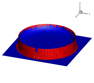
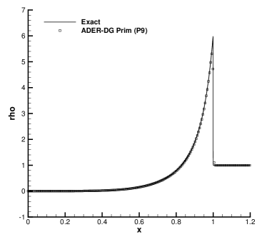
Figure 1: Sedov blast wave problem using an ADER-DG $P9$ scheme with a posteriori subcell finite volume limiter using predictor and limiter in primitive variables, see Zanotti and Dumbser (2016). Unlimited cells are depicted in blue, while limited cells are highlighted in red (left). 1D cut through the numerical solution and comparison with the exact solution (right).

3.2 A novel diffuse interface approach for linear seismic wave propagation in complex geometries

Seismic wave propagation problems in complex 3D geometries are often very challenging due to the geometric complexity. Standard approaches either use regular curvilinear boundary-fitted meshes, or unstructured tetrahedral or hexahedral meshes. In all cases, a certain amount of user interaction for grid generation is required. Furthermore, the geometric complexity can have a negative impact on the admissible time step size due to the CFL condition, since the mesh generator may create elements with very bad aspect ratio, so–called sliver elements. In the case of regular curvilinear grids, the Jacobian of the mapping may become ill-conditioned and thus reduce the admissible time step size. In Tavelli et al. (2018) a novel diffuse interface approach has been forwarded, where only the definition of a scalar volume fraction function $\alpha$ is required, where $\alpha=1$ is set inside the solid medium, and $\alpha=0$ in the surrounding gas or vacuum. The governing PDE system proposed in Tavelli et al. (2018) reads

$$\frac{\partial\boldsymbol{\sigma}}{\partial t}-\mathbf{E}(\lambda,\mu)\cdot\frac{1}{\alpha}\nabla{(\alpha\mathbf{v})}+\frac{1}{\alpha}\mathbf{E}(\lambda,\mu)\cdot{\mathbf{v}}\otimes\nabla\alpha=\mathbf{S}_{\sigma},$$ (21)

$$\frac{\partial{\alpha\mathbf{v}}}{\partial{t}}-\frac{\alpha}{\rho}\nabla\cdot\boldsymbol{\sigma}-\frac{1}{\rho}\boldsymbol{\sigma}\nabla\alpha=\mathbf{S}_{v},$$ (22)

$$\frac{\partial{\alpha}}{\partial{t}}=0,\qquad\frac{\partial{\lambda}}{\partial{t}}=0,\qquad\frac{\partial{\mu}}{\partial{t}}=0,\qquad\frac{\partial{\rho}}{\partial{t}}=0,$$ (23)

and clearly falls into the class of PDE systems described by (1). Here, $\boldsymbol{\sigma}$ denotes the symmetric stress tensor, $\mathbf{v}$ is the velocity vector, $\alpha\in[0,1]$ is the volume fraction, $\lambda$ and $\mu$ are the Lamé constants and $\rho$ is the density of the solid medium. The elasticity tensor $\mathbf{E}$ is a function of $\lambda$ and $\mu$ and relates stress and strain via the Hooke law. The last four quantities obey trivial evolution equations, which state that these parameters remain constant in time. However, they still need to be properly included in the evolution system, since they have an influence on the solution of the Riemann problem. An analysis of the eigenstructure of (21) - (23) shows that the eigenvalues are all real and are independent of the volume fraction function $\alpha$. Furthermore, the exact solution of a generic Riemann problem with $\alpha=1$ on the left and $\alpha=0$ on the right yields the free surface boundary condition $\boldsymbol{\sigma}\cdot\mathbf{n}=0$ at the interface, see Tavelli et al. (2018) for details. In this new approach, the mesh generation problem can be fully avoided, since all that is needed is the specification of the scalar volume fraction function $\alpha$, which is set to unity inside the solid and to zero outside. A realistic 3D wave propagation example based on real DTM data of the Mont Blanc region is shown in Figures 2 and 3, where the 3D contour colors of the wave field as well as a set of seismogram recordings in two receiver points are reported. For this simulation, a uniform Cartesian base-grid of $80^{3}$ elements was used, together with one level of AMR refinement close to the free surface boundary determined by the DTM model. A fourth order ADER-DG scheme ($N=3$) has been used in this simulation. We stress that the entire setup of the computational model in the diffuse interface approach is completely automatic, and no manual user interaction was required. The reference solution was obtained with a high order ADER-DG scheme of the same polynomial degree $N=3$ using an unstructured boundary-fitted tetrahedral mesh Dumbser and Käser (2006) of similar spatial resolution, containing a total of $1,267,717$ elements. We observe an excellent agreement between the two simulations, which were obtained with two completely different PDE systems on two different grid topologies.

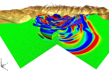
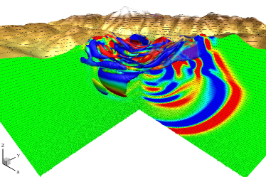
Figure 2: Wave field of a seismic wave propagation problem with the novel diffuse interface approach on adaptive Cartesian grids developed in Tavelli et al. (2018) (left) compared with the reference solution obtained on a classical boundary-fitted unstructured tetrahedral mesh Dumbser and Käser (2006) (right).

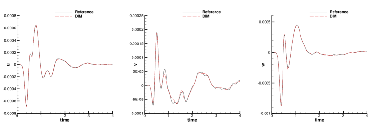
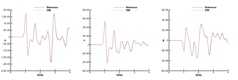
Figure 3: Seismogram recordings in two observation points obtained with the diffuse interface approach on adaptive Cartesian meshes Tavelli et al. (2018) and with a reference solution obtained with high order ADER-DG schemes on boundary-fitted unstructured meshes Dumbser and Käser (2006).

3.3 The unified Godunov-Peshkov-Romenski model of continuum mechanics (GPR)

A major achievement of ExaHyPE was the first successful numerical solution of the unified first order symmetric hyperbolic and thermodynamically compatible Godunov–Peshkov–Romenski (GPR) model of continuum mechanics, see Dumbser et al. (2016, 2017). The GPR model is based on the seminal papers by Godunov and Romenski Godunov et al. (1961); Godunov and Romenski (1972); Romenski (1998) on inviscid symmetric hyperbolic systems. The dissipative mechanisms, which allow to model both plastic solids as well as viscous fluids within one single set of equations were added later in the groundbreaking work of Peshkov and Romenski in Peshkov and Romenski (2016). The GPR model is briefly outlined below, while for all details the interested reader is referred to Peshkov and Romenski (2016); Dumbser et al. (2016, 2017). The governing equations read

$$\frac{\partial\rho}{\partial t}+\frac{\partial}{\partial x_{k}}\left(\rho u_{k}\right)=0,$$ (24)

$$\frac{\partial\rho u_{i}}{\partial t}+\frac{\partial}{\partial x_{k}}\left(\partial\rho u_{i}u_{k}+p\delta_{ik}-\sigma_{ik}\right)=0,$$ (25)

$$\frac{\partial A_{ik}}{\partial t}+\frac{\partial\left(A_{im}u_{m}\right)}{\partial x_{k}}+u_{j}\left(\frac{\partial A_{ik}}{\partial x_{j}}-\frac{\partial A_{ij}}{\partial x_{k}}\right)=-\frac{\psi_{ik}}{\theta_{1}(\tau_{1})},$$ (26)

$$\frac{\partial\rho J_{i}}{\partial t}+\frac{\partial}{\partial x_{k}}\left(\rho J_{i}u_{k}+T\delta_{ik}\right)=-\frac{1}{\theta_{2}(\tau_{2})}\rho H_{i},$$ (27)

$$\frac{\partial\rho E}{\partial t}+\frac{\partial}{\partial x_{k}}\left(u_{k}\rho E+u_{i}\left(p\delta_{ik}-\sigma_{ik}\right)+q_{k}\right)=0.$$ (28)

Furthermore, the system is also endowed with an entropy inequality, see Dumbser et al. (2016). Here, $\rho$ is the mass density, $[u_{i}]=\mathbf{v}=(u,v,w)$ is the velocity vector, $p$ is a non-equilibrium pressure, $[A_{ik}]=\mathbf{A}$ is the distorsion field, $[J_{i}]=\mathbf{J}$ is the thermal impulse vector, $T$ is the temperature and $\rho E$ is the total energy density that is defined according to Dumbser et al. (2016) as

$$\rho E=\rho e+\frac{1}{2}\rho\mathbf{v}^{2}+\frac{1}{4}\rho c_{s}^{2}\,\textnormal{tr}\left((\textnormal{dev}\mathbf{G})^{T}(\textnormal{dev}\mathbf{G})\right)+\frac{1}{2}\rho\alpha^{2}\mathbf{J}^{2}$$ (29)

in terms of the specific internal energy $e=e(p,\rho)$ given by the usual equation of state (EOS), the kinetic energy, the energy stored in the medium due to deformations and in the thermal impulse. Furthermore, $\mathbf{G}=\mathbf{A}^{T}\mathbf{A}$ is a metric tensor induced by the distortion field $\mathbf{A}$, which allows to measure distances and thus deformations in the medium, $c_{s}$ is the shear sound speed and $\alpha$ is a heat wave propagation speed; the symbol $\textnormal{dev}\mathbf{G}=\mathbf{G}-\frac{1}{3}\textnormal{tr}\,\mathbf{G}$ indicates the trace-free part of the metric tensor $\mathbf{G}$. From the definition of the total energy (29) and the relations $H_{i}=E_{J_{i}}$, $\psi_{ik}=E_{A_{ij}}$, $\sigma_{ik}=-\rho A_{mi}E_{A_{mk}}$, $T=E_{S}$ and $q_{k}=E_{S}E_{J_{k}}$ the shear stress tensor and the heat flux read $\boldsymbol{\sigma}=-\rho c_{s}^{2}\mathbf{G}\textnormal{dev}{\mathbf{G}}$ and $\mathbf{q}=\alpha^{2}T\mathbf{J}$. It can furthermore be shown via formal asymptotic expansion Dumbser et al. (2016) that via an appropriate choice of $\theta_{1}$ and $\theta_{2}$ in the stiff relaxation limit $\tau_{1}\to 0$ and $\tau_{2}\to 0$, the stress tensor and the heat flux tend to those of the compressible Navier-Stokes equations

$$\boldsymbol{\sigma}\to\mu\left(\nabla\mathbf{v}+\nabla\mathbf{v}^{T}-\frac{2}{3}\left(\nabla\cdot\mathbf{v}\right)\mathbf{I}\right)\qquad\textnormal{and}\qquad\mathbf{q}\to-\lambda\nabla T,$$ (30)

with transport coefficients $\mu=\mu(\tau_{1},c_{s})$ and $\lambda=\lambda(\tau_{2},\alpha)$ related to the relaxation times $\tau_{1}$ and $\tau_{2}$ and to the propagation speeds $c_{s}$ and $\alpha$, respectively. For a complete derivation, see Dumbser et al. (2016, 2017). In the opposite limit $\tau_{1}\to\infty$ the model describes an ideal elastic solid with large deformations. This means that elastic solids as well as viscous fluids can be described at the aid of the same mathematical model. At this point we stress that numerically we always solve the unified first order hyperbolic PDE system (24)-(28), even in the stiff relaxation limit (30), when the compressible Navier-Stokes-Fourier system is retrieved asymptotically. We emphasize that we never need to discretize any parabolic terms, since the hyperbolic system (24)-(28) with algebraic relaxation source terms fits perfectly into the framework of Eqn. (1).

In the Fig. 4 we show numerical results obtained in Dumbser et al. (2016) for a viscous heat conducting shock wave and the comparison with the exact solution of the compressible Navier-Stokes equations.

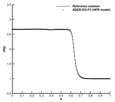
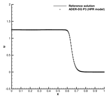
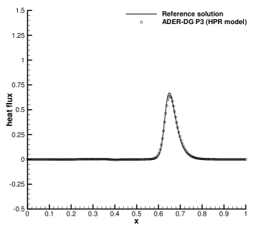
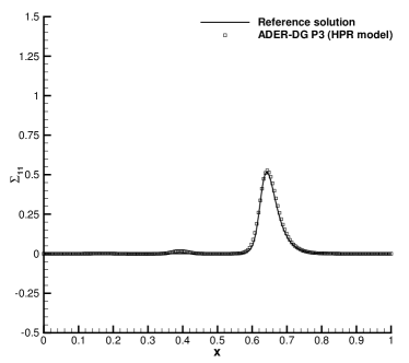
Figure 4: Viscous heat conducting shock. Comparison of the exact solution of the compressible Navier-Stokes equations with the numerical solution of the GPR model based on ADER-DG $P3$ schemes. Density profile (top left), velocity profile (top right), heat flux (bottom left) and stress $\sigma_{11}$ (bottom right).

3.4 The equations of ideal general relativistic magnetohydrodynamics (GRMHD)

A very challenging PDE system is given by the equations of ideal general relativistic magnetohydrodynamics (GRMHD). The governing PDE are a result of the Einstein field equations and can be written in compact covariant notation as follows:

$$\nabla_{\mu}T^{\mu\nu}=0,\qquad\textnormal{and}\qquad\nabla_{\mu}\,^{*}F^{\mu\nu}=0\qquad\textnormal{and}\qquad\nabla_{\mu}(\rho u^{\mu})=0,$$ (31)

where $\nabla_{\mu}$ is the usual covariant derivative operator, $T^{\mu\nu}$ is the energy-momentum tensor, $\,{}^{*}F^{\mu\nu}$ is the Faraday tensor and $u^{\mu}$ is the four-velocity. The compact equations above can be expanded into a so-called 3+1 formalism, which can be cast into the form of (1), see Antón et al. (2006); Zanna et al. (2007); Fambri et al. (2018) for more details. The final evolution system involves 9 field variables plus the 4-metric of the background space-time, which is supposed to be stationary here. A numerical convergence study for the large amplitude Alfvén wave test problem described in Zanna et al. (2007) solved in the domain $\Omega=[0,2\pi]^{3}$ up to $t=1$ and carried out with high order ADER-DG schemes in Fambri et al. (2018) is reported in the Table 2 below, where we also show a direct comparison with high order Runge-Kutta discontinuous Galerkin schemes. We observe that the ADER-DG schemes are competitive with RKDG methods, even for this very complex system of hyperbolic PDE. The results reported in Table 2 refer to the non-vectorized version of the code. Further significant performance improvements are expected from a carefully vectorized implementation of the GRMHD equations, in particular concerning the vectorization of the cumbersome conversion of the vector of conservative variables to the vector of primitive variables, i.e. the function $\mathbf{V}=\mathbf{V}(\mathbf{Q})$. For the GRMHD system $\mathbf{V}$ cannot be computed analytically in terms of $\mathbf{Q}$, but requires the iterative solution of one nonlinear scalar algebraic equation together with the computation of the roots of a third order polynomial, see Zanna et al. (2007) for details. In our vectorized implementation of the PDE, we have therefore in particular vectorized the primitive variable recovery via a direct implementation in AVX intrinsics. We have furthermore made use of careful auto-vectorization via the compiler for the evaluation of the physical flux function and for the non-conservative product. Thanks to this vectorization effort, on one single CPU core of an Intel i9-7900X Skylake test workstation with 3.3 GHz nominal clock frequency and using AVX 512 the CPU time necessary for a single degree of freedom update (TDU) for a fourth order ADER-DG scheme ($N=3$) could be reduced to TDU = 2.3 $\mu$s for the GRMHD equations in three space dimensions.

$N_{x}$	$L_{2}$ error	$L_{2}$ order	WCT [s]	$N_{x}$	$L_{2}$ error	$L_{2}$ order	WCT [s]
ADER-DG ($N=3$)				RKDG ($N=3$)
8	7.6396E-04		0.093	8	8.0909E-04		0.107
16	1.7575E-05	5.44	1.371	16	2.2921E-05	5.14	1.394
24	6.7968E-06	2.34	6.854	24	7.3453E-06	2.81	6.894
32	1.0537E-06	6.48	21.642	32	1.3793E-06	5.81	21.116
ADER-DG ($N=4$)				RKDG ($N=4$)
8	6.6955E-05		0.363	8	6.8104E-05		0.456
16	2.2712E-06	4.88	5.696	16	2.3475E-06	4.86	6.666
24	3.3023E-07	4.76	28.036	24	3.3731E-07	4.78	29.186
32	7.4728E-08	5.17	89.271	32	7.7084E-08	5.13	87.115
ADER-DG ($N=5$)				RKDG ($N=5$)
8	5.2967E-07		1.090	8	5.7398E-07		1.219
16	7.4886E-09	6.14	16.710	16	8.1461E-09	6.14	17.310
24	7.1879E-10	5.78	84.425	24	7.7634E-10	5.80	83.777
32	1.2738E-10	6.01	263.021	32	1.3924E-10	5.97	260.859

Table 2: Accuracy and cost comparison between ADER-DG and RKDG schemes of different orders for the GRMHD equations in three space dimensions. The errors refer to the variable $B_{y}$. The table also contains total wall clock times (WCT) measured in seconds using 512 MPI ranks of the SuperMUC phase I system at the LRZ in Garching, Germany.

As second test problem we present the results obtained for the Orszag-Tang vortex system in flat Minkowski spacetime, where the GRMHD equations reduce to the special relativitic MHD equations. The initial condition is given by

$$\left(\rho,u,v,w,p,B_{x},B_{y},B_{z}\right)=\left(1,-\frac{3}{4\sqrt{2}}\sin y\,,\frac{3}{4\sqrt{2}}\sin x\,,0,1,-\sin y\,,\sin 2x\,,0\right)\,,$$

and we set the adiabatic index to $\Gamma=4/3$. The computational domain is $\Omega=[0,2\pi]^{2}$ and is discretized with a dynamically adaptive AMR grid. For this test we chose the $P_{5}$ version of the ADER-DG scheme with FV subcell limiter and the rest mass density as indicator function for AMR, i.e. $\varphi(\mathbf{Q})=\rho$. Fig. 6 shows 1D cuts through the numerical solution at time $t=2$ and at $y=0.01$, while Fig. 5 shows the numerical results for the AMR-grid with limiter-status map (blue cells are unlimited, while limited cells are highlighted in red), together with Schlieren images for the rest-mass density at time $t=2$. The same simulation has been repeated with different refinement estimator functions $\chi$ that tell the AMR algorithm where and when to refine and to coarsen the mesh: (i) a simple first order derivative estimator $\chi_{1}$ based on discrete gradients of the indicator function $\varphi(\mathbf{Q})$, (ii) the classical second order derivative estimator $\chi_{2}$ based on Löhner (1987), (iii) a novel estimator $\chi_{3}$ based on the action of the a posteriori subcell finite volume limiter, i.e. the mesh is refined where the limiter is active (iv) a multi-resolution estimator $\chi_{4}$ based on the difference in $L_{\infty}$ norm of the discrete solution on two different refinement levels $\ell$ and $\ell-1$. The reference solution is obtained on a uniform fine grid corresponding to the finest refinement level, i.e. a uniform composed of $270\times 270$ elements. The results shown in Fig. 5 clearly show that the numerical results obtained by means of different refinement estimator functions are comparable with each other and thus the proposed AMR algorithm is robust with respect to the particular choice of the mesh.

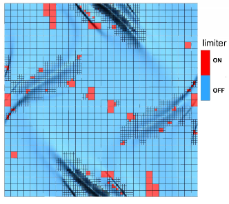
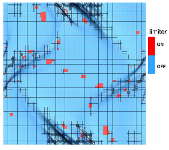
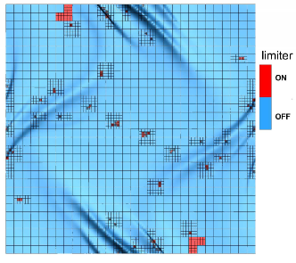
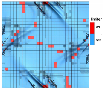
Figure 5: Results for the GRMHD Orszag-Tang vortex problem in flat space-time (SRMHD) at $t=2$ obtained with ADER-DG-$\mathbb{P}_{5}$ schemes, supplemented with a posteriori subcell finite volume limiter and using different refinement estimator functions $\chi$. (i) first order-derivative estimator $\chi_{1}$ (top left); (ii) second-order derivative estimator $\chi_{2}$ (top right); (iii) a new limiter-based estimator $\chi_{3}$ (row 2, left) and (iv) a new multi-resolution estimator $\chi_{4}$ based on the difference between the discrete solution on two adjacent refinement levels (row 2 right).

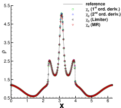
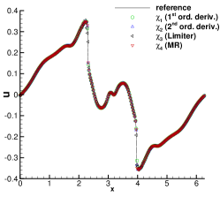
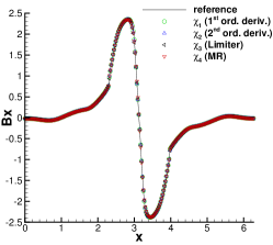
Figure 6: Results for the GRMHD Orszag-Tang vortex problem in flat space-time (SRMHD) at $t=2$ obtained with ADER-DG-$\mathbb{P}_{5}$ schemes supplemented with a posteriori subcell finite volume limiter and using different refinement estimator functions $\chi$. A set of 1D cuts taken at $y=10^{-2}$ are shown. From left to right: the rest-mass density, the velocity $u$ and the magnetic field component $B_{x}$. One can note an excellent agreement between the reference solution and the ones obtained on different AMR grids.

As last test case we simulate a stationary neutron star in three space dimensions using the Cowling approximation, i.e. assuming a fixed static background spacetime. The initial data for the matter and the spacetime are both compatible with the Einstein field equations and are given by the solution of the Tolman–Oppenheimer–Volkoff (TOV) equations, which constitute a nonlinear ODE system in the radial coordinate that can be numerically solved up to any precision at the aid of a fourth order Runge-Kutta scheme using a very fine grid. We setup a stable nonrotating TOV star without magnetic field and with central rest mass density $\rho(\mathbf{0},0)=1.28\cdot 10^{-3}$ and adiabatic exponent $\Gamma=2$ in a computational domain $\Omega=[-10,+10]^{3}$ discretized with a fourth order ADER-DG scheme ($N=3$) using $32^{3}$ elements, which corresponds to $128^{3}$ spatial degrees of freedom. The pressure in the atmosphere outside the compact object is set to $p_{atm}=10^{-13}$. We run the simulation until a final time of $t=1000$ and measure the $L_{\infty}$ error norms of the rest mass density and the pressure against the exact solution, which is given by the initial condition. The error at $t=1000$ for the rest mass density is $L_{\infty}(\rho)=1.553778\cdot 10^{-5}$ while the error for the pressure is $L_{\infty}(p)=1.605334\cdot 10^{-7}$. The simulation was carried out with the vectorized version of the code on 512 CPU cores of the SuperMUC phase 2 system (based on AVX2) and required only 3010 s of wallclock time. The same simulation with the established finite difference GR code WhiskyTHC Radice et al. (2014) required 8991 s of wall clock time on the same machine with the same spatial mesh resolution and the same number of CPU cores. The time series of the relative error of the central rest mass density in the origin of the domain is plotted in the left panel of Fig. 7. At the final time $t=1000$, the relative error of the central rest mass density is still below 0.1%. In the right panel of Fig. 7 we show the contour surfaces of the pressure at the final time $t=1000$. In Fig. 8 we show a 1D cut along the $x$ axis, comparing the numerical solution at time $t=1000$ with the exact one. We note that the numerical scheme is very accurate, but it is not well-balanced for the GRMHD equations, i.e. the method cannot preserve the stationary equilibrium solution of the TOV equations exactly at the discrete level. Therefore, further work along the lines of research reported recently in Gaburro et al. (2018) for the Euler equations with Newtonian gravity are needed, extending the framework of well-balanced methods Bermúdez and Vázquez (1994); Castro et al. (2006); Parés (2006) also to general relativity. Finally, in Fig. 9 we compare the exact and the numerical solution at time $t=1000$ in the $x-y$ plane.

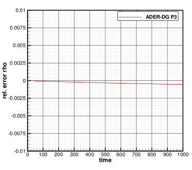
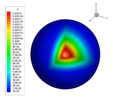
Figure 7: Computational results for a stable 3D neutron star. Time series of the relative error of the central rest mass density $\left(\rho(\mathbf{0},t)-\rho(\mathbf{0},0)\right)/\rho(\mathbf{0},0)$ (left) and 3D view of of the pressure contour surfaces at time $t=1000$ (right).

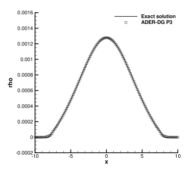
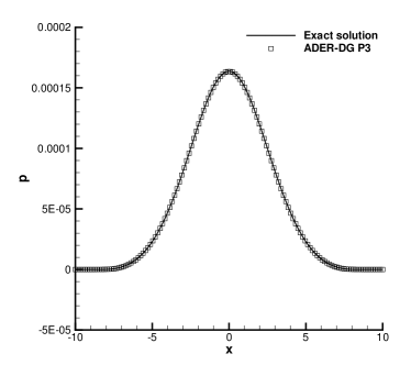
Figure 8: Computational results for a stable 3D neutron star. Comparison of the numerical solution with the exact one at time $t=1000$ on a 1D cut along the $x$-axis for the rest mass density (left) and the pressure (right).

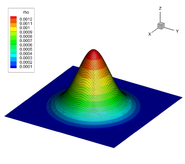
Figure 9: Computational results for a stable 3D neutron star. Cut through the $x-y$ plane with pressure on the $z$ axis and rest mass density contour colors. Exact solution (left) and numerical solution at time $t=1000$ (right).

3.5 A strongly hyperbolic first order reduction of the CCZ4 formulation of the Einstein field equations (FO-CCZ4)

The last PDE system under consideration here are the Einstein field equations that describe the evolution of dynamic spacetimes. Here we consider the so-called CCZ4 formulation Alic et al. (2012), which is based on the Z4 formalism that takes into account the involutions (stationary differential constraints) inherent in the Einstein equations via an augmented system similar to the generalized Lagrangian multiplier (GLM) approach of Dedner et al. Dedner et al. (2002) that takes care of the stationary divergence-free constraint of the magnetic field in the MHD equations. In compact covariant notation the undamped Z4 Einstein equations in vacuum, which can be derived from the Einstein-Hilbert action integral associated with the Z4 Lagrangian $\mathcal{L}=g^{\mu\nu}\left(R_{\mu\nu}+2\nabla_{\mu}Z\nu\right)$, read

$$R_{\mu\nu}+\nabla_{(\mu}Z_{\nu)}=0,$$ (32)

where $g^{\mu\nu}$ is the 4-metric of the spacetime, $R_{\mu\nu}$ is the 4-Ricci tensor and the 4-vector $Z_{\nu}$ accounts for the stationary constraints of the Einstein equations, as already mentioned before. After introducing the usual 3+1 ADM split of the 4-metric as

$$ds^{2}=-\alpha^{2}dt^{2}+\gamma_{ij}\left(dx^{i}+\beta^{i}dt\right)\left(dx^{j}+\beta^{j}dt\right),$$ (33)

the equations can be cast into a time-dependent system of 25 partial differential equations that involve first order derivatives in time and both first and second order derivatives in space, see Alic et al. (2012). Nevertheless, the system is not dissipative, but a rather unusual formulation of a wave equation, see Gundlach and Martin-Garcia (2004). In the expression above, $\alpha$ denotes the so-called lapse, $\beta^{i}$ is the spatial shift vector and $\gamma_{ij}$ is the spatial metric. In the original form presented in Alic et al. (2012), the PDE system does not fit into the formalism given by Eqn. (1). After the introduction of 33 auxiliary variables, which are the spatial gradients of some of the 25 primary evolution quantities, it is possible to derive a first order reduction of the system that contains a total of 58 evolution quantities. However, a naive procedure of converting the original second order evolution system into a first order system leads only to a weakly hyperbolic formulation, which is not suitable for numerical simulations since the initial value problem is not well posed in this case. Only after adding suitable first and second order ordering constraints, which arise from the definition of the auxiliary variables, it is possible to obtain a provably strongly hyperbolic and thus well-posed evolution system, denoted by FO-CCZ4 in the following. For all details of the derivation, the strong hyperbolicity proof and numerical results achieved with high order ADER-DG schemes, the reader is referred to Dumbser et al. (2018). In order to give an idea about the complexity of the Einstein field equations, it should be mentioned that one single evaluation of the FO-CCZ4 system requires about 20,000 floating point operations! In order to obtain still a computationally efficient implementation, the entire PDE system has been carefully vectorized using blocks of the size VECTORLENGTH, so that in the end a level of 99,9 % of vectorization of the code have been reached. Using a fourth order ADER-DG scheme ($N=3$) the time per degree of freedom update (TDU) metric per core on a modern workstation with Intel i9-7900X CPU that supports the novel AVX 512 instructions is TDU=4.7 $\mu$s.

4 Strong MPI scaling study for the FO-CCZ4 system

A major focus of this paper is the efficient implementation of ADER-DG schemes for high performance computing (HPC) on massively parallel distributed memory supercomputers. For this purpose, we have very recently carried out a systematic study of the strong MPI scaling efficiency of our new high order fully-discrete one-step ADER-DG schemes on the Hazel Hen supercomputer of the HLRS center in Stuttgart, Germany, using from 720 up to 180,000 CPU cores. We have furthermore carried out a systematic comparison with conventional Runge-Kutta DG schemes using the SuperMUC phase 1 system of the LRZ center in Munich, Germany.

As already discussed before, the particular feature of ADER-DG schemes compared to traditional Runge-Kutta DG schemes (RKDG) is that they are intrinsically communication-avoiding and cache-blocking, which makes them particularly well suited for modern massively parallel distributed memory supercomputers. As governing PDE system for the strong scaling test the novel first-order reduction of the CCZ4 formulation of the 3+1 Einstein field equations has been been adopted Dumbser et al. (2018). We recall that FO-CCZ4 is a very large nonlinear hyperbolic PDE system that contains 58 evolution quantities.

The first strong scaling study on the SuperMUC phase 1 system uses 64 to 64,000 CPU cores. The test problem was the gauge wave problem Dumbser et al. (2018) setup on the 3D domain $\Omega=[-0.5,0.5]^{3}$. For the test we have compared a fourth order ADER-DG scheme ($N=3$) with a fourth order accurate RKDG scheme on a uniform Cartesian grid composed of $120^{3}$ elements. It has to be stressed, that when using 64,000 CPU cores for this setup each CPU has to update only $3^{3}=27$ elements. The wall clock time as a function of the used number of CPU cores (nCPU) and the obtained parallel efficiency with respect to an ideal linear scaling are reported in the left panel of Fig. 10. We find that ADER-DG schemes provide a better parallel efficiency than RKDG schemes, as expected.

The second strong scaling study has been performed on the Hazel-Hen supercomputer, using 720 to 180,000 CPU cores. Again we have used a fourth order accurate ADER-DG scheme ($N=3$), this time using a uniform grid of $200\times 180\times 180$ elements, solving again the 3D gauge wave benchmark problem detailed in Dumbser et al. (2018). The measured wall-clock-times (WCT) as a function of the employed number of CPU cores, as well as the corresponding parallel scaling-efficiency are shown in Fig. 10. The results depicted in Fig. 10 clearly show that our new ADER-DG schemes scale very well up to 90,000 CPU cores with a parallel efficiency greater than 95%, and up to 180,000 cores with a parallel efficiency that is still greater than 93%. Furthermore, the code was instrumented with manual FLOP counters in order to measure the floating point performance quantitatively. The full machine run on 180,000 CPU cores of Hazel Hen took place on 7th of May 2018. During the run, each core has provided an average performance of 8.2 GFLOPS, leading to a total of 1.476 PFLOPS of sustained performance. To our knowledge, this was the largest test run ever carried out with high order ADER-DG schemes for nonlinear hyperbolic systems of partial differential equations. For large runs with sustained petascale performance of ADER-DG schemes for linear hyperbolic PDE systems on unstructured tetrahedral meshes, see Breuer et al. (2014b).

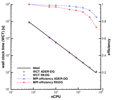
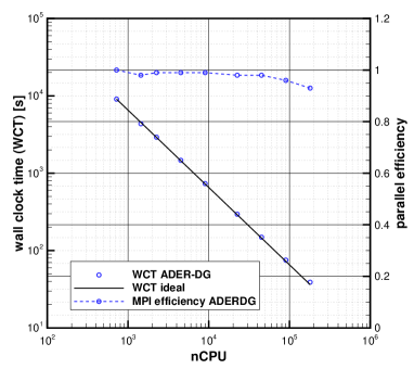
Figure 10: Strong MPI scaling study of ADER-DG schemes for the novel FO-CCZ4 formulation of the Einstein field equations recently proposed in Dumbser et al. (2018). Left: comparison of ADER-DG schemes with conventional Runge-Kutta DG schemes from 64 to 64,000 CPU cores on the SuperMUC phase 1 system of the LRZ supercomputing center (Garching, Germany). Right: strong scaling study from 720 to 180,000 CPU cores, including a full machine run on the Hazel Hen supercomputer of HLRS (Stuttgart, Germany) with ADER-DG schemes (right). Even on the full machine we observe still more than 90 % of parallel efficiency.

5 Conclusions

In this paper we have presented an efficient implementation of high order ADER-DG schemes on modern massively parallel supercomputers using the ExaHyPE engine. The key ingredients are the communication-avoiding and cache-blocking properties of ADER-DG, together with an efficient vectorization of the high level user functions that provide the evaluation of the physical fluxes $\mathbf{F}(\mathbf{Q})$, of the non-conservative products $\mathbf{B}(\mathbf{Q})\cdot\nabla\mathbf{Q}$ and of the algebraic source terms $\mathbf{S}(\mathbf{Q})$. The engine is highly versatile and flexible and allows to solve a very broad spectrum of different hyperbolic PDE systems in a very efficient and highly scalable manner. In order to support this claim, we have provided a rather large set of different numerical examples solved with ADER-DG schemes. To show the excellent parallel scalability of the ADER-DG method, we have provided strong scaling results on 64 to 64,000 CPU cores including a detailed and quantitative comparison with RKDG schemes. We have furthermore shown strong scaling results of the vectorized ADER-DG implementation for the FO-CCZ4 formulation of the Einstein field equations using 720 to 180,000 CPU cores of the Hazel Hen supercomputer at the HLRS in Stuttgart, Germany, where a sustained performance of more than one petaflop has been reached.

Future research in ExaHyPE will concern an extension of the GPR model to full general relativity, able to describe nonlinear elastic and plastic solids as well as viscous and ideal fluids in one single governing PDE system. We furthermore plan an implementation of the FO-CCZ4 system Dumbser et al. (2018) directly based on AVX intrinsics, in order to further improve the performance of the scheme and to reduce computational time. The final aim of our developments are the simulation of ongoing nonlinear dynamic rupture processes during earthquakes, as well as the inspiral and merger of binary neutron star systems and the associated generation of gravitational waves. Although both problems seem to be totally different and unrelated, it is indeed possible to write the mathematical formulation of both applications under the same form of a hyperbolic system given by (1) and thus to solve both problems within the same computer software.

“Conceptualization and Methodology: M.D., M.B. and T.W.; Software: M.D., T.W., F.F. and M.T.; Validation: F.F. and M.T.; Strong MPI Scaling Study: F.F; Writing original draft and editing: M.D.; Supervision and Project Administration: M.B., T.W. and M.D.; Funding Acquisition: M.B., T.W. and M.D. ”.

This research was funded by the European Union’s Horizon 2020 Research and Innovation Programme under the project ExaHyPE, grant no. 671698 (call FETHPC-1-2014). The first three authors also acknowledge funding from the Italian Ministry of Education, University and Research (MIUR) in the frame of the Departments of Excellence Initiative 2018–2022 attributed to DICAM of the University of Trento. MD also acknowledges support from the University of Trento in the frame of the Strategic Initiative Modeling and Simulation.