Walker solution for Dzyaloshinskii domain wall in ultrathin ferromagnetic films

Abstract

We analyze the electric current and magnetic field driven domain wall motion in perpendicularly magnetized ultrathin ferromagnetic films in the presence of interfacial Dzyaloshinskii-Moriya interaction and both out-of-plane and in-plane uniaxial anisotropies. We obtain exact analytical Walker-type solutions in the form of one-dimensional domain walls moving with constant velocity due to both spin-transfer torques and out-of-plane magnetic field. These solutions are embedded into a larger family of propagating solutions found numerically. Within the considered model, we find the dependencies of the domain wall velocity on the material parameters and demonstrate that adding in-plane anisotropy may produce domain walls moving with velocities in excess of 500 m/s in realistic materials under moderate fields and currents.

Introduction. In their seminal paper, Schryer and Walker discovered an exact analytical solution of the Landau-Lifshitz-Gilbert (LLG) equation describing a moving one-dimensional (1D) domain wall (DW) Schryer and Walker (1974). In this so-called Walker solution, the magnetization rotates in a fixed plane determined by the material parameters and magnetic field, connecting the two opposite in-plane equilibrium orientations of magnetization. The Walker solution has since been used in numerous problems of DW motion to successfully explain the physics of magnetization reversal Atkinson et al. (2003); Yamaguchi et al. (2004); Allwood et al. (2005); Hayashi et al. (2008); Tatara and Kohno (2004); Duine et al. (2007); Tretiakov et al. (2008); Yang et al. (2009); Boone et al. (2010); Tretiakov and Ar. Abanov (2010); Khvalkovskiy et al. (2013); Shibata et al. (2011); Hoffmann and Bader (2015).

Recently, out-of-plane magnetized ultrathin films with Dzyaloshinskii-Moriya interaction (DMI) Dzyaloshinsky (1958); Moriya (1960) have attracted significant interest Thiaville et al. (2012); Boulle et al. (2013); Emori et al. (2013a); Ryu et al. (2013); Brataas (2013); Torrejon et al. (2014); Emori et al. (2013b); Franken et al. (2014); Martinez et al. (2014); Vandermeulen et al. (2016); Yu et al. (2016) due to their potential advantages for high-performance spinorbitronic devices Miron et al. (2011); Emori et al. (2013b); Yoshimura et al. (2016). These materials are known to exhibit chiral DWs Yoshimura et al. (2016); Soumyanarayanan et al. (2016); Garg et al. (2018), but so far no explicit dynamic Walker-type solution has been demonstrated to exist, which significantly hinders understanding of the DW motion in these systems.

In this Rapid Communication, we report a new exact analytical solution for steady DW motion in out-of-plane magnetized films analogous to the Walker solution for films with in-plane equilibrium magnetization. For this solution to exist, a small in-plane anisotropy is required in addition to the dominant out-of-plane anisotropy, while the film is still magnetized out-of-plane. We consider both current and field driven DW dynamics in the presence of interfacial DMI and show that this new solution can describe the DW motion observed in recent experiments Emori et al. (2013b); Franken et al. (2014); Yu et al. (2016).

At nonzero DMI strength, our solution fixes the angle of magnetization in the DW such that it acquires a strictly Néel profile. The solution also fixes the angle between the direction of the current and the DW normal. This angle depends on the relative strength of magnetic field and electric current, but, notably, is independent of the DMI strength. Moreover, in the absence of DMI we find an entire family of exact solutions for every angle between the DW normal and the in-plane easy axis. Although the dynamics in biaxial ferromagnets has been the subject of many works (see, e.g., Kosevich et al. (1990); Thiaville et al. (2005); Goussev et al. (2013); Su et al. (2017); Nasseri et al. (2018)), the interplay between DMI and biaxial anisotropy leads to additional interesting phenomena.

We also demonstrate that one can achieve the highest propagation velocities for tiltless DWs, i. e., DWs which move along the current with the DW front strictly perpendicular to the current (Fig. 1), by appropriately tuning the magnetic field. As a result, we provide an exact experimentally relevant Boulle et al. (2013); Emori et al. (2013b); Franken et al. (2014); Yu et al. (2016) way to achieve the maximal DW velocity in a nanowire for a given current. We note that in thin nanowires, the direction of current along the wire coincides with the direction of the in-plane easy-axis shape anisotropy due to stray fields Kohn and Slastikov (2005).

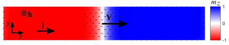
Figure 1: A snapshot of tiltless DW driven by current $\mathbf{j}$ and out-of-plane magnetic field $\mathbf{h}$ in a ferromagnetic nanostrip with DMI and two anisotropies (larger out-of-plane and smaller in-plane along the strip axis) from a simulation of Eq. (1).

Model. We consider an ultrathin ferromagnetic film of thickness $d$ with interfacial DMI and two anisotropies: larger out-of-plane and smaller in-plane, and study the dynamic behavior of magnetic DWs due to an out-of-plane magnetic field and/or in-plane electric current. Our analysis is based on the LLG equation with spin-transfer torques Tatara and Kohno (2004); Thiaville et al. (2005) describing the evolution of the reduced magnetization $\mathbf{m}(\mathbf{r},t)$ sup :

$$\frac{\partial\mathbf{m}}{\partial t}=\mathbf{h}_{\rm{eff}}\times\mathbf{m}+\alpha\mathbf{m}\times\frac{\partial\mathbf{m}}{\partial t}-(\mathbf{j}\cdot\nabla)\mathbf{m}+\beta\mathbf{m}\times(\mathbf{j}\cdot\nabla)\mathbf{m},$$ (1)

where $\mathbf{r}\in\mathbb{R}^{2}$ is the spatial coordinate in units of the exchange length $\ell_{ex}=\sqrt{2A/(\mu_{0}M_{s}^{2})}$ and $t$ is time in the units of $(\gamma\mu_{0}M_{s})^{-1}$, $A$ is the exchange stiffness, $M_{s}$ is the saturation magnetization, $\gamma$ is the gyromagnetic ratio, $\alpha$ is the Gilbert damping constant, $\beta$ is the nonadiabatic spin-transfer torque constant, $\mathbf{j}=\hbar P\mathbf{J}/\sqrt{8Ae^{2}\mu_{0}M_{s}^{2}}$, $\mathbf{J}$ is the in-plane current density, $P$ is the spin polarization of current, and $\mathbf{h}_{\textrm{eff}}=-\delta E/\delta\mathbf{m}$ with energy $E$ in units of $2Ad$ given by

$$\!\!E(\mathbf{m})= \frac{1}{2}\int_{\mathbb{R}^{2}}\Big{[}|\nabla\mathbf{m}|^{2}+(k_{z}-1)(1-m_{z}^{2})-k_{x}m_{x}^{2}$$

$$-2{h_{z}}m_{z}+\kappa\left(m_{z}\nabla\cdot\mathbf{m}^{\prime}-\mathbf{m}^{\prime}\cdot\nabla m_{z}\right)\Big{]}\,d^{2}r.$$ (2)

Here $\mathbf{m}=(\mathbf{m}^{\prime},m_{z})$, $\mathbf{m}^{\prime}=(m_{x},m_{y})$, and we introduced the dimensionless parameters corresponding to the dimensional out-of-plane and in-plane anisotropy constants $K_{z}$ and $K_{x}$, interfacial DMI constant $D$, and out-of-plane field $H_{z}$, respectively:

$$k_{x,z}={2K_{x,z}\over\mu_{0}M_{s}^{2}},\quad\kappa=D\sqrt{2\over\mu_{0}M_{s}^{2}A},\quad h_{z}={H_{z}\over M_{s}}.$$ (3)

We assume $k_{z}>1$ and $0<k_{x}<k_{z}-1$ to ensure that $\mathbf{m}=\pm\hat{\mathbf{z}}$ are the only stable equilibria for $h_{z}=0$. The energy in Eq. (Walker solution for Dzyaloshinskii domain wall in ultrathin ferromagnetic films) is appropriate for ultrathin films, i. e., for $d/\ell_{ex}\ll 1$ Muratov et al. (2017). Note that Eq. (1) does not include spin-orbit torques, which may be important in bilayer/multilayer ferromagnetic structures with heavy-metal layers, where electric currents run in the presence of strong spin-orbit interaction Garello et al. (2013); Ado et al. (2017); Manchon et al. (2018); Ramaswamy et al. (2018). However, spin-orbit torques affect not just the DW itself, but the entire magnetization configuration in the film, thus precluding the existence of Walker-type solutions.

DW profile. We study the dynamics of DWs moving due to either an applied magnetic field or a spin-transfer torque from an electric current. By a moving DW with normal velocity $V$ in the direction of the unit vector $\hat{\mathbf{n}}=(n_{x},n_{y})$ we mean a 1D solution of (1) of the form $\mathbf{m}=\mathbf{m}(\mathbf{r}\cdot\hat{\mathbf{n}}-Vt)$. Substituting this traveling wave ansatz into Eq. (1) and writing $\mathbf{m}=(\sin\theta\cos\phi,\sin\theta\sin\phi,\cos\theta)$ yields the following system of differential equations for $\theta$ and $\phi$ as functions of $\xi=\mathbf{r}\cdot\hat{\mathbf{n}}-Vt$ sup :

$$\frac{1}{\sin\theta}\frac{d}{d\xi}\!\left(\!\sin^{2}\theta\frac{d\phi}{d\xi}\!\right)\!+\!(\alpha V\!-\!\beta\mathbf{j}\cdot\hat{\mathbf{n}})\sin\theta\frac{d\phi}{d\xi}$$

$$\!-\!(\mathbf{j}\cdot\hat{\mathbf{n}}\!-\!V\!+\!\kappa\hat{\mathbf{n}}\cdot\hat{\mathbf{p}}\sin\theta)\frac{d\theta}{d\xi}-\frac{k_{x}}{2}\sin\theta\sin 2\phi=0,$$ (4)

$$\frac{d^{2}\theta}{d\xi^{2}}\!+\!(\alpha V\!-\!\beta\mathbf{j}\cdot\hat{\mathbf{n}})\frac{d\theta}{d\xi}\!+\!(\mathbf{j}\cdot\hat{\mathbf{n}}\!-\!V\!+\!\kappa\hat{\mathbf{n}}\cdot\hat{\mathbf{p}}\sin\theta)\sin\theta\frac{d\phi}{d\xi}$$

$$\!-\!\left(\!k_{z}\!-\!1+\!\left|\frac{d\phi}{d\xi}\right|^{2}\!-\!k_{x}\cos^{2}\phi\!\right)\!\sin\theta\cos\theta\!-\!h_{z}\sin\theta\!=0,\!$$ (5)

where for convenience we defined $\hat{\mathbf{p}}=(-\sin\phi,\cos\phi)$. Equations (Walker solution for Dzyaloshinskii domain wall in ultrathin ferromagnetic films) and (Walker solution for Dzyaloshinskii domain wall in ultrathin ferromagnetic films) need to be supplemented by the conditions at infinity. With the convention that the positive velocity ($V>0$) corresponds to a domain with $\mathbf{m}=-\hat{\mathbf{z}}$ invading the domain with $\mathbf{m}=\hat{\mathbf{z}}$, we require $\theta(-\infty)=\pi$ and $\theta(+\infty)=0$. The DW velocity $V$ is determined by solvability of Eqs. (Walker solution for Dzyaloshinskii domain wall in ultrathin ferromagnetic films) and (Walker solution for Dzyaloshinskii domain wall in ultrathin ferromagnetic films).

Walker solution. In the absence of DMI ($\kappa=0$), Eqs. (Walker solution for Dzyaloshinskii domain wall in ultrathin ferromagnetic films) and (Walker solution for Dzyaloshinskii domain wall in ultrathin ferromagnetic films) admit an exact solution for every $\hat{\mathbf{n}}$ with the help of the Walker ansatz Schryer and Walker (1974), thereby generalizing the results of Ref. Goussev et al. (2013) to two-dimensional (2D) film. Namely, setting $\phi=\phi_{0}=\mathrm{const}$ and matching the second derivative of $\theta(\xi)$ to the term proportional to $\sin 2\theta$ yields

$$h_{z}\sin\theta-(\alpha V-\beta\mathbf{j}\cdot\hat{\mathbf{n}})\theta^{\prime} =0,$$ (6)

$$\theta^{\prime\prime}-(k_{z}-1-k_{x}\cos^{2}\phi_{0})\sin\theta\cos\theta =0,$$ (7)

$$(V-\mathbf{j}\cdot\hat{\mathbf{n}})\theta^{\prime}-\tfrac{1}{2}k_{x}\sin\theta\sin 2\phi_{0} =0,$$ (8)

where $\theta^{\prime}=d\theta/d\xi$ and $\theta^{\prime\prime}=d^{2}\theta/d\xi^{2}$. This system of equations produces a Walker-type solution for a steadily moving DW:

$$\theta(\xi)=2\arctan e^{-\xi\sqrt{k_{z}-1-k_{x}\cos^{2}\phi_{0}}},$$ (9)

propagating with velocity

$$V=-{h_{z}\over\alpha\sqrt{k_{z}-1-k_{x}\cos^{2}\phi_{0}}}+{\beta\mathbf{j}\cdot\hat{\mathbf{n}}\over\alpha},$$ (10)

where $\phi_{0}$ solves

$$\mathbf{j}\cdot\hat{\mathbf{n}}(\alpha\!-\!\beta)\sqrt{k_{z}\!-\!1\!-\!k_{x}\cos^{2}\phi_{0}}\!+\!h_{z}\!=\!\tfrac{1}{2}\alpha k_{x}\sin 2\phi_{0}.$$ (11)

The obtained front velocity depends on the propagation direction $\hat{\mathbf{n}}$, unless $\mathbf{j}\cdot\hat{\mathbf{n}}=0$. In particular, at $h_{z}=0$ the velocity is maximal in the direction of $\mathbf{j}$. The solution exists only when $|h_{z}|$ and $j=|\mathbf{j}|$ do not exceed critical values corresponding to Walker breakdown Schryer and Walker (1974); Clarke et al. (2008); Goussev et al. (2013).

In the presence of DMI ($\kappa\not=0$) the Walker solution obtained above is generally destroyed. Nevertheless, Eqs. (6)–(8) are preserved in the special case when $\phi_{0}$ is chosen so that $\hat{\mathbf{n}}\cdot\hat{\mathbf{p}}=0$. This condition is equivalent to

$$\hat{\mathbf{n}}=\pm(\cos\phi_{0},\sin\phi_{0}),$$ (12)

corresponding to a Néel-type DW profile, in which the magnetization rotates entirely in the $\hat{\mathbf{n}}$-$\hat{\mathbf{z}}$ plane. We stress that Eq. (12) is dictated by solvability of Eqs. (6)–(8) and is not an assumption. In terms of the space-time variables, the solution is given by

$$\mathbf{m}(\mathbf{r},t)=(\pm\hat{\mathbf{n}}\sin\theta(\mathbf{r}\cdot\hat{\mathbf{n}}-Vt),\cos\theta(\mathbf{r}\cdot\hat{\mathbf{n}}-Vt)),$$ (13)

where $\theta$ is given by Eq. (9), and “$\pm$” corresponds to the choice of the sign in Eq. (12). This is an exact Walker-type solution valid in the presence of interfacial DMI and describing a 1D moving DW. Its propagation direction is given by Eq. (12) in which $\phi_{0}$ solves

$$h_{z}-\tfrac{1}{2}\alpha k_{x}\sin 2\phi_{0}\pm(\alpha-\beta)(j_{x}\cos\phi_{0}+j_{y}\sin\phi_{0})$$

$$\times\sqrt{k_{z}-1-k_{x}\cos^{2}\phi_{0}}=0,$$ (14)

for $\mathbf{j}=(j_{x},j_{y})$, according to Eq. (11). In general, Eq. (Walker solution for Dzyaloshinskii domain wall in ultrathin ferromagnetic films) reduces to a fourth-order equation in $\cos^{2}\phi_{0}$, whose roots can in principle be found for all parameters. Below we consider two important cases of purely current or field driven DW motion, which are simpler mathematically and contain all the essential physics.

Before concentrating on moving DWs, we consider the case of no applied field and current, corresponding to static DWs (for further details, see, e.g., Ref. Rohart and Thiaville (2013)). With $h_{z}=j=0$, Eq. (Walker solution for Dzyaloshinskii domain wall in ultrathin ferromagnetic films) yields four distinct solutions: $\phi_{0}=-{\pi\over 2},0,{\pi\over 2},\pi$. Then, inserting the profile from Eq. (13) with $V=0$ into Eq. (Walker solution for Dzyaloshinskii domain wall in ultrathin ferromagnetic films), one obtains the static DW energy per unit length

$$E_{0}=2\sqrt{k_{z}-1-k_{x}\cos^{2}\phi_{0}}\mp\tfrac{1}{2}\kappa\pi.$$ (15)

The DW energy $E_{0}$ is positive and is minimized by $\phi_{0}=0,\pi$ for $|\kappa|<(4/\pi)\sqrt{k_{z}-1-k_{x}}$. Furthermore, the DMI contribution is minimized by the “$+$” sign in Eq. (12) when $\kappa>0$, and by the “$-$” sign when $\kappa<0$. These minimizing choices of $\phi_{0}$ and the sign in Eq. (12) yield global minimizers (up to translations) of the 1D DW energy under the conditions $\theta(-\infty)=\pi$ and $\theta(+\infty)=0$ for Eqs. (Walker solution for Dzyaloshinskii domain wall in ultrathin ferromagnetic films) and (Walker solution for Dzyaloshinskii domain wall in ultrathin ferromagnetic films), since in this case both the DMI and the in-plane anisotropy energy contributions are separately minimized Muratov and Slastikov (2016). Thus, the choices of $\hat{\mathbf{n}}$ dictated by Eq. (12) with the above choices of $\phi_{0}$ and the sign correspond to the DW orientations with the lowest $E_{0}$.

We now consider two characteristic cases of moving DWs. For definiteness, we assume $\kappa>0$ and fix the positive sign in Eq. (12), corresponding to the minimum of the static DW energy. It then allows us to think of $\phi_{0}$ as the angle defining the normal vector in the direction of DW propagation whenever $V>0$. In the simplest case of no current, we find that for $|h_{z}|\leq h_{z}^{c}$ the propagation angle of a DW solving Eq. (Walker solution for Dzyaloshinskii domain wall in ultrathin ferromagnetic films) satisfies

$$\sin 2\phi_{0}=2h_{z}/(\alpha k_{x}),\qquad h_{z}^{c}=\alpha k_{x}/2.$$ (16)

Once again, this equation produces four distinct values of $\phi_{0}\in(-\pi,\pi]$ for $|h_{z}|$ below the Walker breakdown field $h_{z}^{c}$. Due to the symmetry $\phi_{0}\to\phi_{0}+\pi$, $\hat{\mathbf{n}}\to-\hat{\mathbf{n}}$ for $j=0$, this still results in two distinct solutions (differing by 180^∘ rotations) with propagation velocities determined by Eq. (10). For both values, the sign of $V$ coincides with that of $-h_{z}$, while the magnitude of $V$ is maximized by $\phi_{0}=\tfrac{1}{2}\arcsin[2h_{z}/(\alpha k_{x})]$. This choice corresponds to the branch of solutions that connects to the global DW energy minimizers as $h_{z}\to 0$ and should thus correspond to the physically observed solution. The DW velocity is

$$V=-\frac{h_{z}}{\alpha\sqrt{k_{z}-1-\frac{k_{x}}{2}\left(1+\sqrt{1-{4h_{z}^{2}\over\alpha^{2}k_{x}^{2}}}\,\right)}}.$$ (17)

In particular, the velocity $V$ and angle $\phi_{0}$ at small fields grow linear in $h_{z}$, while for $|h_{z}|$ comparable to $h_{z}^{c}$ they acquire a nonlinear character. The magnitude of $|\phi_{0}|$ is a monotonically increasing function of $|h_{z}|$, whose maximum $|\phi_{0}|=\pi/4$ is achieved at the Walker breakdown field $|h_{z}|=h_{z}^{c}$. Also, the DMI part of the DW energy is, in fact, globally minimized by our sign choice in Eq. (12).

Next, we study the case of purely current driven DW motion with $\mathbf{j}=(j_{x},0)$ along the in-plane easy axis. By Eq. (Walker solution for Dzyaloshinskii domain wall in ultrathin ferromagnetic films) one DW solution corresponds to a profile with $V=0$ and $\phi_{0}=\pm\pi/2$. For $|j_{x}|<j_{x}^{c}$, where the critical ”Walker breakdown” current is

$$j_{x}^{c}=\alpha k_{x}/(|\alpha-\beta|\sqrt{k_{z}-1}),$$ (18)

Eq. (Walker solution for Dzyaloshinskii domain wall in ultrathin ferromagnetic films) has two additional solutions:

$$\phi_{0}=\arcsin\left({(\alpha-\beta)j_{x}\over k_{x}}\sqrt{\frac{k_{x}(k_{z}-1-k_{x})}{\alpha^{2}k_{x}-j_{x}^{2}\left(\alpha-\beta\right)^{2}}}\,\right),$$ (19)

and another one obtained by changing $\phi_{0}\to\pi-\phi_{0}$ (and $V\to-V$ in the equation for the velocity). Focusing on the first solution and substituting the angle from Eq. (19) into Eq. (10), we obtain

$$V=\frac{\beta j_{x}}{\alpha}\sqrt{\alpha^{2}k_{x}^{2}-j_{x}^{2}(\alpha-\beta)^{2}(k_{z}-1)\over\alpha^{2}k_{x}^{2}-j_{x}^{2}(\alpha-\beta)^{2}k_{x}}.$$ (20)

In the purely current driven case the DW velocity in the horizontal direction $V_{x}=V/\cos\phi_{0}$ takes a universal form $V_{x}=\beta j_{x}/\alpha$ [see Eq. (10)] also found for current-induced DW and skyrmion motion in other systems Thiaville et al. (2005); Goussev et al. (2013, 2016); Barker and Tretiakov (2016). In particular, the DW is driven only by the non-adiabatic torque. As $j_{x}$ is increased, the angle $\phi_{0}$ monotonically increases, first linearly in $j_{x}$ and then acquiring a nonlinear character closer to its maximum $|\phi_{0}|={\pi\over 2}$ at $|j_{x}|=j_{x}^{c}$. For larger currents one would expect $|\phi_{0}|$ to remain equal to $\pi/2$, consistent with the above static DW solution.

Other traveling-wave solutions. As we just demonstrated, the Walker-type solutions obtained for $\kappa\not=0$ exist only for certain specific directions of propagation determined by the solutions of Eqs. (Walker solution for Dzyaloshinskii domain wall in ultrathin ferromagnetic films) and (12). In contrast, for $\kappa=0$ there exists a traveling wave solution for every direction $\hat{\mathbf{n}}$, provided that $h_{z}$ and $j$ are not too large. To investigate this further, we carried out numerical simulations of the 1D version of Eq. (1) with initial condition $\mathbf{m}(\mathbf{r},0)=(\hat{\mathbf{n}}\,\textrm{sech}(\frac{1}{2}\mathbf{r}\cdot\hat{\mathbf{n}}),\tanh(\frac{1}{2}\mathbf{r}\cdot\hat{\mathbf{n}}))$, where $\hat{\mathbf{n}}$ is given by Eq. (12) with the “+” sign, and determined the long-time asymptotic DW profile. For all parameter choices used in our simulations the solution always converged to a DW moving with a constant velocity $V=V(\phi_{0})$. In particular, for every propagation direction we found a propagating DW solution, which coincided with the Walker-type solution obtained above for the particular propagation direction satisfying Eq. (Walker solution for Dzyaloshinskii domain wall in ultrathin ferromagnetic films). We illustrate our findings with simulation results for the material parameters as in Boulle et al. (2013): $A=10^{-11}$ J/m, $M_{s}=1.09\times 10^{6}$ A/m, $K_{z}=1.25\times 10^{6}$ J/m³, $D=1$ mJ/m², and $\alpha=0.5$.

With no current, we carried out simulations for in-plane anisotropy constant $K_{x}=0.125\times 10^{6}$ J/m³ and applied field $\mu_{0}H_{z}=-25$ mT, corresponding to $|h_{z}|$ comparable to the Walker breakdown field $h_{z}^{c}$ and a relatively small $k_{x}$ sup . We then obtained the DW profile and velocity as functions of propagation direction. The profile was found to be close to that of the Walker solution, coinciding with it exactly when $\phi_{0}$ solves Eq. (Walker solution for Dzyaloshinskii domain wall in ultrathin ferromagnetic films). A plot of $V(\phi_{0})$ is presented in Fig. 2, indicating the points corresponding to the Walker solution with green dots.

For small values of $k_{x}$ the DW moves with velocity nearly independent of direction and its magnitude is close to the velocity of the Walker solution. In this case the DW velocity’s dependence on propagation angle, $V(\phi_{0})$, is well approximated by Eq. (10). On the other hand, as the value of $k_{x}$ is increased, the velocity begins to exhibit a substantial dependence on propagation angle and deviates from the prediction of Eq. (10), except for the Walker solution, even if the latter still gives a fairly good approximation to its magnitude. When $k_{x}$ approaches its maximum value of $k_{z}-1$ the velocity exhibits a strong directional dependence that is not captured by Eq. (10), except, once again, for the Walker solution. Note that the original dimensional propagation velocity $V\sqrt{2A\mu_{0}\gamma_{0}^{2}}$ reaches $\sim\!500$ m/s. Thus, the effect of a large in-plane uniaxial anisotropy is to accelerate the DW by promoting the magnetization rotation in the easy in-plane direction.

Similar results were obtained for current driven DW motion with no applied field. For example, for $K_{x}=0.4\times 10^{6}$ J/m³, $\beta=0.25$, $P=1$, and $J_{x}=5\times 10^{12}$ A/m², we found that the DW velocity is given by Eq. (10) with $h_{z}=0$. This is consistent with the expected physical picture that the DW is advected with the velocity $V_{x}=\beta j_{x}/\alpha$ along the current direction.

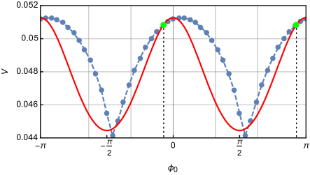
Figure 2: The dimensionless DW velocity $V$ at zero current as a function of the propagation angle $\phi_{0}$ obtained from the solution of Eq. (1) for $k_{z}=1.674$, $k_{x}=0.167$, $\kappa=0.366$, $\alpha=0.5$, and $h_{z}=-0.0183$ corresponding to the parameters in the text. The simulated data are indicated by the blue dots connected with a dashed blue line. The red solid line shows the dependence given by Eq. (10) with $\mathbf{j}=0$. The green dots indicate the velocity for the Walker solution from Eq. (17), corresponding to the special values of $\phi_{0}$ obtained from Eq. (16) and indicated by dotted lines.

Motion along the in-plane easy axis. The analysis of the Walker solution performed above indicates that one can also select the Walker solution moving in a prescribed direction given by angle $\phi_{0}$ via an appropriate choice of the relationship between $h_{z}$ and $\mathbf{j}$. Furthermore, according to Eq. (10), for fixed $h_{z}<0$ and $j$ the maximum velocity of the Walker solution is achieved for $j_{y}=\phi_{0}=0$. Substituting this into Eqs. (Walker solution for Dzyaloshinskii domain wall in ultrathin ferromagnetic films) and (10) then yields

$$V=j_{x}\quad\text{for}\quad h_{z}=j_{x}(\beta-\alpha)\sqrt{k_{z}-1-k_{x}}.$$ (21)

This maximal velocity turns out to be independent of most of the material parameters, and the required field $h_{z}$ vanishes in the special case $\alpha=\beta$. Furthermore, these solutions correspond to moving DWs with no tilt, contrary to those seen in Ref. Boulle et al. (2013) without in-plane anisotropy.

Traveling waves for zero damping. It is interesting that the obtained Walker solution also allows one to construct steadily moving DW solutions at zero damping, $\alpha=0$, for any angle $\phi_{0}$ by taking the limit $\alpha\to 0$, while choosing $h_{z}$ to satisfy Eq. (16) with $\mathbf{j}=0$. Substituting this into Eq. (10) yields yet another exact solution valid for $j=h_{z}=\alpha=0$, in the form of a DW moving with velocity

$$V=-{k_{x}\sin\phi_{0}\cos\phi_{0}\over\sqrt{k_{z}-1-k_{x}\cos^{2}\phi_{0}}},$$ (22)

in the direction of $\hat{\mathbf{n}}$ in Eq. (12) and with profile given by Eq. (13). This solution represents a 1D solitary wave propagating in the direction characterized by $\phi_{0}$ in the Hamiltonian setting, in the presence of interfacial DMI.

2D simulations. To illustrate the role of the obtained DW solutions in magnetization reversal, we carried out full numerical simulations of Eq. (1) in a nanostrip. The onset of a tiltless DW propagation due to both current and out-of-plane field is given in the Supplemental Material movie . A snapshot of the steadily moving DW from this simulation is shown in Fig. 1. We used the same parameters as in 1D simulations above sup . The initial state was a single Néel DW across the strip at $j=h_{z}=0$. In the simulation we then applied both current along $\hat{\mathbf{x}}$ and field along $\hat{\mathbf{z}}$. For the Néel DW in which $\mathbf{m}$ goes from $+\hat{\mathbf{z}}$ through $+\hat{\mathbf{x}}$ to $-\hat{\mathbf{z}}$ from left to right (see Fig. 1), the current and field both drive the DW in the same direction (to the right). We observe that the solution quickly approaches a nearly 1D steadily propagating DW profile corresponding to the Walker type solution constructed above.

Conclusions. We have studied the model of ultrathin ferromagnetic film with interfacial DMI and two magnetic anisotropies. When the out-of-plane anisotropy is stronger than the in-plane anisotropy, we have found an exact 2D traveling wave DW solution [Eqs. (9) and (13)] driven by both electric current and magnetic field. This solution is an analog of the well-known Walker solution for a 1D steadily moving DW. The presence of an in-plane anisotropy is crucial to stabilize this solution, and moreover it allows us to find analytical expressions for the DW propagation direction and velocity [see Eqs. (12) and (Walker solution for Dzyaloshinskii domain wall in ultrathin ferromagnetic films)] as functions of all material parameters.

Acknowledgments. O. A. T. acknowledges support by the Grants-in-Aid for Scientific Research (Grants No. 17K05511 and No. 17H05173) from the Ministry of Education, Culture, Sports, Science and Technology (MEXT), Japan, MaHoJeRo grant (DAAD Spintronics network, Project No. 57334897), by the grant of the Center for Science and Innovation in Spintronics (Core Research Cluster), Tohoku University, and by JSPS and RFBR under the Japan-Russian Research Cooperative Program. C. B. M. was supported by NSF via Grant No. DMS-1614948. V. V. S. and J. M. R. would like to acknowledge support from Leverhulme Trust Grant No. RPG-2014-226.

References

- Schryer and Walker (1974) N. L. Schryer and L. R. Walker, J. Appl. Phys. 45, 5406 (1974).
- Atkinson et al. (2003) D. Atkinson, D. A. Allwood, G. Xiong, M. D. Cooke, C. C. Faulkner, and R. P. Cowburn, Nat. Mater. 2, 85 (2003).
- Yamaguchi et al. (2004) A. Yamaguchi, T. Ono, S. Nasu, K. Miyake, K. Mibu, and T. Shinjo, Phys. Rev. Lett. 92, 077205 (2004).
- Allwood et al. (2005) D. A. Allwood, G. Xiong, C. C. Faulkner, D. Atkinson, D. Petit, and R. P. Cowburn, Science 309, 1688 (2005).
- Hayashi et al. (2008) M. Hayashi, L. Thomas, R. Moriya, C. Rettner, and S. S. Parkin, Science 320, 209 (2008).
- Tatara and Kohno (2004) G. Tatara and H. Kohno, Phys. Rev. Lett. 92, 086601 (2004).
- Duine et al. (2007) R. A. Duine, A. S. Núñez, and A. H. MacDonald, Phys. Rev. Lett. 98, 056605 (2007).
- Tretiakov et al. (2008) O. A. Tretiakov, D. Clarke, G.-W. Chern, Y. B. Bazaliy, and O. Tchernyshyov, Phys. Rev. Lett. 100, 127204 (2008).
- Yang et al. (2009) S. A. Yang, G. S. D. Beach, C. Knutson, D. Xiao, Q. Niu, M. Tsoi, and J. L. Erskine, Phys. Rev. Lett. 102, 067201 (2009).
- Boone et al. (2010) C. T. Boone, J. A. Katine, M. Carey, J. R. Childress, X. Cheng, and I. N. Krivorotov, Phys. Rev. Lett. 104, 097203 (2010).
- Tretiakov and Ar. Abanov (2010) O. A. Tretiakov and Ar. Abanov, Phys. Rev. Lett. 105, 157201 (2010).
- Khvalkovskiy et al. (2013) A. V. Khvalkovskiy, V. Cros, D. Apalkov, V. Nikitin, M. Krounbi, K. A. Zvezdin, A. Anane, J. Grollier, and A. Fert, Phys. Rev. B 87, 020402 (2013).
- Shibata et al. (2011) J. Shibata, G. Tatara, and H. Kohno, J. Phys. D: Appl. Phys. 44, 384004 (2011).
- Hoffmann and Bader (2015) A. Hoffmann and S. D. Bader, Phys. Rev. Appl. 4, 047001 (2015).
- Dzyaloshinsky (1958) I. Dzyaloshinsky, J. Phys. Chem. Solids 4, 241 (1958).
- Moriya (1960) T. Moriya, Phys. Rev. 120, 91 (1960).
- Thiaville et al. (2012) A. Thiaville, S. Rohart, É. Jué, V. Cros, and A. Fert, EPL 100, 57002 (2012).
- Boulle et al. (2013) O. Boulle, S. Rohart, L. D. Buda-Prejbeanu, E. Jué, I. M. Miron, S. Pizzini, J. Vogel, G. Gaudin, and A. Thiaville, Phys. Rev. Lett. 111, 217203 (2013).
- Emori et al. (2013a) S. Emori, U. Bauer, S.-M. Ahn, E. Martinez, and G. S. D. Beach, Nat. Mater. 12, 611 (2013a).
- Ryu et al. (2013) K.-S. Ryu, L. Thomas, S.-H. Yang, and S. S. P. Parkin, Nat. Nanotech. 8, 527 (2013).
- Brataas (2013) A. Brataas, Nat. Nanotech. 8, 485 (2013).
- Torrejon et al. (2014) J. Torrejon, J. Kim, J. Sinha, S. Mitani, M. Hayashi, M. Yamanouchi, and H. Ohno, Nat. Commun. 5, 4655 (2014).
- Emori et al. (2013b) S. Emori, U. Bauer, S.-M. Ahn, E. Martinez, and G. S. D. Beach, Nat. Mater. 12, 611 (2013b).
- Franken et al. (2014) J. H. Franken, M. Herps, H. J. M. Swagten, and B. Koopmans, Sci. Rep. 4, 5248 (2014).
- Martinez et al. (2014) E. Martinez, S. Emori, N. Perez, L. Torres, and G. S. D. Beach, J. Appl. Phys. 115, 213909 (2014).
- Vandermeulen et al. (2016) J. Vandermeulen, S. A. Nasseri, B. V. de Wiele, G. Durin, B. V. Waeyenberge, and L. Dupré, J. Phys. D: Appl. Phys. 49, 465003 (2016).
- Yu et al. (2016) J. Yu, X. Qiu, Y. Wu, J. Yoon, P. Deorani, J. M. Besbas, A. Manchon, and H. Yang, Sci. Rep. 6, 32629 (2016).
- Miron et al. (2011) I. M. Miron, T. Moore, H. Szambolics, L. D. Buda-Prejbeanu, S. Auffret, B. Rodmacq, S. Pizzini, J. Vogel, M. Bonfim, A. Schuhl, and G. Gaudin, Nat. Mater. 10, 419 (2011).
- Yoshimura et al. (2016) Y. Yoshimura, K.-J. Kim, T. Taniguchi, T. Tono, K. Ueda, R. Hiramatsu, T. Moriyama, K. Yamada, Y. Nakatani, and T. Ono, Nat. Phys. 12, 157 (2016).
- Soumyanarayanan et al. (2016) A. Soumyanarayanan, N. Reyren, A. Fert, and C. Panagopoulos, Nature 539, 509 (2016).
- Garg et al. (2018) C. Garg, A. Pushp, S.-H. Yang, T. Phung, B. P. Hughes, C. Rettner, and S. S. P. Parkin, Nano Lett. 18, 1826 (2018).
- Kosevich et al. (1990) A. Kosevich, B. Ivanov, and A. Kovalev, Phys. Rep. 194, 117 (1990).
- Thiaville et al. (2005) A. Thiaville, Y. Nakatani, J. Miltat, and Y. Suzuki, EPL 69, 990 (2005).
- Goussev et al. (2013) A. Goussev, R. G. Lund, J. M. Robbins, V. Slastikov, and C. Sonnenberg, Proc. R. Soc. Lond. Ser. A Math. Phys. Eng. Sci. 469, 20130308 (2013).
- Su et al. (2017) Y. Su, L. Weng, W. Dong, B. Xi, R. Xiong, and J. Hu, Sci. Rep. 7, 13416 (2017).
- Nasseri et al. (2018) S. A. Nasseri, E. Martinez, and G. Durin, J. Magn. Magn. Mater. 468, 25 (2018).
- Kohn and Slastikov (2005) R. V. Kohn and V. V. Slastikov, Arch. Ration. Mech. Anal. 178, 227 (2005).
- (38) See Supplemental Material at [URL to be inserted by publisher], Sec. I for the details of micromagnetic energy and LLG equation modifications; Sec. II for more detailed comparison of the simulation results for small, intermediate, and large values of ; Sec. III for other details of 2D simulations including boundary conditions etc.
- Muratov et al. (2017) C. B. Muratov, V. V. Slastikov, A. G. Kolesnikov, and O. A. Tretiakov, Phys. Rev. B 96, 134417 (2017).
- Garello et al. (2013) K. Garello, I. M. Miron, C. O. Avci, F. Freimuth, Y. Mokrousov, S. Blugel, S. Auffret, O. Boulle, G. Gaudin, and P. Gambardella, Nature Nanotech. 8, 587 (2013).
- Ado et al. (2017) I. A. Ado, O. A. Tretiakov, and M. Titov, Phys. Rev. B 95, 094401 (2017).
- Manchon et al. (2018) A. Manchon, I. M. Miron, T. Jungwirth, J. Sinova, J. Zelezný, A. Thiaville, K. Garello, and P. Gambardella, ArXiv:1801.09636 (2018).
- Ramaswamy et al. (2018) R. Ramaswamy, J. M. Lee, K. Cai, and H. Yang, Appl. Phys. Rev. 5, 031107 (2018).
- Clarke et al. (2008) D. J. Clarke, O. A. Tretiakov, G.-W. Chern, Y. B. Bazaliy, and O. Tchernyshyov, Phys. Rev. B 78, 134412 (2008).
- Rohart and Thiaville (2013) S. Rohart and A. Thiaville, Phys. Rev. B 88, 184422 (2013).
- Muratov and Slastikov (2016) C. B. Muratov and V. V. Slastikov, Proc. R. Soc. Lond. Ser. A 473, 20160666 (2016).
- Goussev et al. (2016) A. Goussev, J. M. Robbins, V. Slastikov, and O. A. Tretiakov, Phys. Rev. B 93, 054418 (2016).
- Barker and Tretiakov (2016) J. Barker and O. A. Tretiakov, Phys. Rev. Lett. 116, 147203 (2016).
- Note (1) See Supplemental Material at [URL to be inserted by publisher] for the movie demonstrating the DW propagation due to both applied field and electric current using micromagnetic simulations.