Relaxed Multirate Infinitesimal Step Methods for Initial-Value Problems

Abstract

This work focuses on the construction of a new class of fourth-order accurate methods for multirate time evolution of systems of ordinary differential equations. We base our work on the Recursive Flux Splitting Multirate (RFSMR) [1, 2, 3] version of the Multirate Infinitesimal Step (MIS) methods [4, 5, 6, 7, 8], and use recent theoretical developments for Generalized Additive Runge-Kutta methods [9, 10] to propose our higher-order Relaxed Multirate Infinitesimal Step extensions. The resulting framework supports a range of attractive properties for multirate methods, including telescopic extensions, subcycling, embeddings for temporal error estimation, and support for changes to the fast/slow time-scale separation between steps, without requiring any sacrifices in linear stability. In addition to providing rigorous theoretical developments for these new methods, we provide numerical tests demonstrating convergence and efficiency on a suite of multirate test problems.

1 Introduction

Increasingly, computational science requires large-scale simulations that consistently and accurately couple distinct physical processes. While the mathematical models for individual processes often have a well-known type (hyperbolic, parabolic, etc.) and are suitable for classical numerical integrators, the same cannot be said for the coupled models. These multiphysics models are often of mixed type, may have limited differentiability, and involve processes that evolve at dissimilar rates. As such, many multiphysics simulations require more flexible time integrators that may be tuned for these complex problems.

In this work, we consider systems of autonomous ordinary differential equations that may be characterized by two distinct dynamical time scales, one “fast” and the other “slow”,

$$y^{\prime}(t) =f^{\left\{s\right\}}(y)+f^{\left\{f\right\}}(y),\quad t_{0}\leq t\leq t_{f},$$ (1)

$$y(t_{0}) =y_{0}\in\mathbb{R}^{n}.$$

We note that this additive form of the problem does not prohibit multirate applications where the solution variables are also partitioned between the two scales,

$$\begin{bmatrix}y_{s}^{\prime}\\ y_{f}^{\prime}\end{bmatrix}=\begin{bmatrix}\overline{f}_{s}\left(y_{s},y_{f}\right)\\ \overline{f}_{f}\left(y_{s},y_{f}\right)\end{bmatrix},\quad t_{0}\leq t\leq t_{f}$$

$$y_{s}(t_{0})=y_{s,0}\in\mathbb{R}^{m},\quad y_{f}(t_{0})=y_{f,0}\in\mathbb{R}^{n-m}$$

$$\Rightarrow$$ (2)

$$y=\begin{bmatrix}y_{s}\\ y_{f}\end{bmatrix},\quad f^{\left\{s\right\}}(y)=\begin{bmatrix}\overline{f}_{s}\\ 0\end{bmatrix},\quad f^{\left\{f\right\}}(y)=\begin{bmatrix}0\\ \overline{f}_{f}\end{bmatrix}.$$

Multirate algorithms evolve the initial-value problem (1) using different time step sizes for the fast and slow processes. For such methods to result in efficiency improvements over more traditional single-rate methods that evolve all processes at the fast time scale, the slow right-hand side function $f^{\left\{s\right\}}$ must be significantly more costly than $f^{\left\{f\right\}}$.

In this work, we consider multirate methods where the slow operator is integrated explicitly and the fast operator is integrated either explicitly or implicitly. To simplify our presentation, we denote the characteristic time-scales of the slow and fast components of the multirate problem as $\overline{dt}_{s}$ and $\overline{dt}_{f}$, respectively. We define the time-scale separation between these as $\overline{m}=\overline{dt}_{s}/\overline{dt}_{f}$. We integrate these components using the time-step sizes ${dt}_{s}=h$ and ${dt}_{f}=h/m$, where $m$ is the smallest integer satisfying $\overline{m}<m$. We note that other authors weaken this restriction, by allowing for variable step sizes at the fast time scale [11]. While the methods proposed here may be easily extended to such situations, the focus of this paper is on the construction of higher-order methods; investigations of adaptive fast substepping are left for future work.

As with single-rate problems, the order of accuracy of a multirate method describes how the error behaves as $h\to 0$. Within the multirate context, this overall error arises from multiple sources: the error in the evolution of the fast components, the error in the evolution of the slow components, and the coupling error between the two scales. For a variety of multirate methods, the fast component method is a composition of $m$ steps of a fast base method, while the slow component method is one step of a slow base method – in this case the multirate method order depends on the order of both base methods and on the coupling order.

1.1 Runge–Kutta Theory for Multirate Methods

In recent work, Sandu and Günther introduced a theory for Generalized-Structure Additively-Partitioned Runge-Kutta (GARK) methods [10, 12]. As the name suggests, this theory may be applied to understand a wide range of Runge-Kutta-like time integration methods, and notably provides both order conditions and a linear stability theory for methods in this general format. For simplicity, GARK methods are formulated for autonomous systems of ODEs in additively-split form,

$$\frac{dy}{dt}=f(y)=\sum_{q=1}^{N}f^{\left\{q\right\}}\left(y\right).$$

Here, we consider the case of $N=2$, corresponding to our target problems (1), i.e.

$$\frac{dy}{dt}=f^{\{f\}}\left(y\right)+f^{\{s\}}\left(y\right).$$

Here, GARK methods are uniquely determined by coefficients in an expanded Butcher tableau,

$$\begin{array}[]{c|c}{\mathbf{A}}^{\left\{f,f\right\}}&{\mathbf{A}}^{\left\{f,s\right\}}\\ \hline\cr{\mathbf{A}}^{\left\{s,f\right\}}&{\mathbf{A}}^{\left\{s,s\right\}}\\ \hline\cr\hline\cr{{\mathbf{b}}^{\left\{f\right\}\intercal}}&{{\mathbf{b}}^{\left\{s\right\}\intercal}}\end{array}$$ (6)

where internal stages and solution update are given by

$${k}^{\left\{{f}\right\}}_{j} =y_{n}+h\sum_{l=1}^{s^{\{f\}}}{a}^{\left\{{f,f}\right\}}_{j,l}f^{\{f\}}\left({k}^{\left\{{f}\right\}}_{l}\right)+h\sum_{l=1}^{s^{\{s\}}}{a}^{\left\{{f,s}\right\}}_{j,l}f^{\{s\}}\left({k}^{\left\{{s}\right\}}_{l}\right),$$

$${k}^{\left\{{s}\right\}}_{i} =y_{n}+h\sum_{l=1}^{s^{\{f\}}}{a}^{\left\{{s,f}\right\}}_{i,l}f^{\{f\}}\left({k}^{\left\{{f}\right\}}_{l}\right)+h\sum_{l=1}^{s^{\{s\}}}{a}^{\left\{{s,s}\right\}}_{i,l}f^{\{s\}}\left({k}^{\left\{{s}\right\}}_{l}\right),$$ (7)

$$y_{n+1} =y_{n}+h\sum_{l=1}^{s^{\{f\}}}{b}^{\left\{{f}\right\}}_{l}f^{\{f\}}\left({k}^{\left\{{f}\right\}}_{l}\right)+h\sum_{l=1}^{s^{\{s\}}}{b}^{\left\{{s}\right\}}_{l}f^{\{s\}}\left({k}^{\left\{{s}\right\}}_{l}\right),$$

in which the slow stage indices range over $i=1,\dots,s^{\{s\}}$ and the fast stage indices range over $j=1,\dots,s^{\{f\}}$. In particular, we note that this constitutes a “hybrid” of partitioned Runge-Kutta (PRK) and additive Runge-Kutta (ARK) formulations: there are distinct stages for each right-hand side component (PRK-like), and all right-hand side functions are used to update each stage (ARK-like).

As is typical for additive Runge-Kutta methods, Sandu and Günther make the simplifying assumption of internal consistency, i.e.

$${c}^{\left\{{q}\right\}}_{i}=\sum_{j=1}^{s^{\{f\}}}{a}^{\left\{{q,f}\right\}}_{i,j}=\sum_{j=1}^{s^{\{s\}}}{a}^{\left\{{q,s}\right\}}_{i,j}\qquad\forall\,i=1,\ldots,s^{\{q\}},\quad q=f,s.$$ (8)

Order conditions for methods up to fourth order (and for GARK tableau of arbitrary size) are provided in matrix-vector form in [10, 12], and additionally in elementwise form in [12]. As our work focuses on the derivation of a new class of fourth order methods, we reproduce their matrix-vector form here, where we assume internal consistency (8):

$${{\mathbf{b}}^{\left\{\sigma\right\}\intercal}}\mathbbm{1}^{\{\sigma\}} =1,$$ (9)

$${{\mathbf{b}}^{\left\{\sigma\right\}\intercal}}{\mathbf{c}}^{\left\{\sigma\right\}} =\frac{1}{2},$$ (10)

$${{\mathbf{b}}^{\left\{\sigma\right\}\intercal}}\left({\mathbf{c}}^{\left\{\sigma\right\}}\times{\mathbf{c}}^{\left\{\sigma\right\}}\right) =\frac{1}{3},$$ (11)

$${{\mathbf{b}}^{\left\{\sigma\right\}\intercal}}{\mathbf{A}}^{\left\{\sigma,\nu\right\}}{\mathbf{c}}^{\left\{\nu\right\}} =\frac{1}{6},$$ (12)

$${{\mathbf{b}}^{\left\{\sigma\right\}\intercal}}\left({\mathbf{c}}^{\left\{\sigma\right\}}\times{\mathbf{c}}^{\left\{\sigma\right\}}\times{\mathbf{c}}^{\left\{\sigma\right\}}\right) =\frac{1}{4},$$ (13)

$$\left({\mathbf{b}}^{\left\{\sigma\right\}}\times{\mathbf{c}}^{\left\{\sigma\right\}}\right)^{\intercal}{\mathbf{A}}^{\left\{\sigma,\nu\right\}}{\mathbf{c}}^{\left\{\nu\right\}} =\frac{1}{8},$$ (14)

$${{\mathbf{b}}^{\left\{\sigma\right\}\intercal}}{\mathbf{A}}^{\left\{\sigma,\nu\right\}}\left({\mathbf{c}}^{\left\{\nu\right\}}\times{\mathbf{c}}^{\left\{\nu\right\}}\right) =\frac{1}{12},$$ (15)

$${{\mathbf{b}}^{\left\{\sigma\right\}\intercal}}{\mathbf{A}}^{\left\{\sigma,\mu\right\}}{\mathbf{A}}^{\left\{\mu,\nu\right\}}{\mathbf{c}}^{\left\{\nu\right\}} =\frac{1}{24}.$$ (16)

In these formulas, $\sigma$, $\nu$ and $\mu$ each range over the values $\{f,s\}$, and we denote a column vector of ones in $\mathbb{R}^{s^{\{\sigma\}}}$ as $\mathbbm{1}^{\{\sigma\}}$. Throughout this manuscript we denote standard matrix and vector multiplication with adjacent objects (e.g., $\mathbf{b}^{\intercal}\mathbf{c}$ is an inner product), and we use the $\times$ operator or exponents to denote component-wise multiplication (e.g., for $\mathbf{b},\mathbf{c}\in\mathbb{R}^{n}$ then $(\mathbf{b}\times\mathbf{c})_{i}=b_{i}c_{i}$ and $(\mathbf{b}^{2})_{i}=b_{i}b_{i}$ for $i=1,\ldots,n$). We note that of the above equations, (9) corresponds to the order 1 conditions, (10) corresponds to the order 2 conditions, (11)-(12) correspond to the order 3 conditions, and (13)-(16) correspond to the order 4 conditions. Hence for a two-component splitting, a fourth order method requires 28 order conditions to be met. As with [13], we categorize these order conditions into two groups: all conditions that include ${\mathbf{b}}^{\left\{f\right\}}$ (i.e., the 14 conditions (9)-(16) with $\sigma=f$) are considered as “fast order conditions”, and the rest based on ${\mathbf{b}}^{\left\{s\right\}}$ are considered as “slow order conditions.”

1.2 Multirate Background

Multirate methods and the understanding of their order and stability properties have evolved over time; however the GARK framework can be used to describe and analyze the full history of multirate methods having Runge–Kutta type [13]. In this section, we first give a summary of the historical context of multirate methods, and in the following section we discuss specifics of how to apply GARK theory to these methods.

The first multirate methods were introduced by Gear and Wells in the early 1980’s [14, 15, 16]; these methods integrated only a single scale at a time, using linear interpolation to provide data from one time scale to the other. This work was extended by Constantinescu and Sandu to construct second order multirate methods based on explicit linear multistep base methods [17, 18].

A more general approach to construction of third-order multirate methods was introduced in 1999 by Kværnø [19], and was further elaborated by many authors [20, 21, 22, 23]. In these approaches, one assumes a partitioned formulation with variables split into active (fast) and latent (slow). From here, higher-order interpolants between the two components are obtained by interleaving the interpolation processes between the fast and slow scales. A particular strength of this work is their derivation of a set of simplifying assumptions, so that once these are satisfied and the base method is third order, the resulting multirate method will also be third order. More recently, Fok and Rosales constructed linearly fourth-order multirate methods using higher-order interpolation between the slow and fast stages of a particular Runge-Kutta base method [24].

An alternate approach for higher-order multirate schemes has been pursued through extrapolation of lower-order methods. The first such work is from Engstler and Lubich’s 1997 paper [25], that generated higher-order solutions by extrapolating first-order methods. The efficiency of these methods was subsequently improved through use of dense output formulas [25, 26, 27]. More recent methods of this type, including explicit fast and explicit slow integration (explicit/explicit), as well as implicit fast and explicit slow integration (implicit/explicit), have been explored by Constantinescu and Sandu [28, 29], who investigated extrapolation from first-order accurate methods. These multirate extrapolation approaches increase the possible order of the method at the cost of repeated evaluations of the same time step. Hence, although these methods are reasonable for improvement one or two orders of accuracy, they may become cost-prohibitive when generating higher-order methods.

Each of these approaches has included some effort to develop methods which enforce desirable properties based on the originating PDE problem. Several papers have been published which investigate the coupling of finite element discretizations with multirate schemes [30, 31, 32]. Constantinescu and Sandu introduce methods which focus on preserving conservation properties for PDEs [17]. Schlegel also posited some mass-preserving methods [1], that focus on conservation of linear invariants in the multirate scheme.

In [13], Günther and Sandu not only analyzed many of the aforementioned multirate methods using GARK theory, but also proposed a general infrastructure for constructing multirate GARK (MrGARK) methods. In a recent preprint [33], Sarshar and collaborators utilize this framework to develop a set of fourth-order explicit/explicit multirate GARK methods, through construction of the coefficient matrices ${\mathbf{A}}^{\left\{f,s\right\}}$ and ${\mathbf{A}}^{\left\{s,f\right\}}$ to directly address the coupling conditions between two fourth-order base methods. That work additionally proposes a novel approach for multirate time adaptivity, through construction of various sets of embedding coefficients to separately measure the errors at the slow and fast time scales, as well as the coupling error between scales.

Our work builds most closely off of recent work in Multirate Infinitesimal Step (MIS) methods. Originally developed by Wensch, Knoth and Galant, MIS methods were constructed as a generalization of split-explicit methods in the context of numerical weather prediction [8, 34, 35]. A key contribution from [8] was the development of a systematic approach to the order conditions for split-explicit methods based on PRK theory [8], allowing the development of second and third order MIS methods for a variety of applications [1, 2, 3, 4, 5, 6, 7, 8]. The basic approach of these methods is that the slow right-hand side function $f^{\left\{s\right\}}$ is evaluated to provide forcing terms to create a sequence of modified initial-value problems at the fast time scale,

$$v^{\prime}(\tau)=f^{\{f\}}(\tau,v)+\sum_{j=1}^{i}\alpha_{i,j}f^{\{s\}}(t_{n}+c_{j}h,Y_{j}^{\{s\}}),$$ (17)

$$v(t_{n}+c_{i}h)=Y_{i}^{\{s\}},$$

where $\tau\in[t_{n}+c_{i}h,t_{n}+c_{i+1}h]$, $i$ ranges over the stages at the slow time scale, and where the coefficients $\alpha_{i,j}\in\mathbb{R}$ are defined based on the slow Butcher tableau. In particular, we highlight the development of the Recursive Flux-Splitting Multirate (RFSMR) methods in [1] based on this MIS theory. RFSMR methods are a specialization of MIS methods which leverage a recursive formulation of the differential equations at different scales in order to improve parallel performance.

Very recently, Sandu has posted a preprint that also extends MIS methods to higher order [36]. In his proposed Multirate Infinitesimal GARK (MRI-GARK) approach, Sandu changes the formulation of the modified initial-value problems at the fast time scale (17) to instead create a time-dependent forcing function based off of the slow right-hand side evaluations,

$$v^{\prime}(\tau)=f^{\{f\}}(\tau,v)+\sum_{j=1}^{i+1}\gamma_{i,j}(\tau)f^{\{s\}}(t_{n}+c_{j}h,Y_{j}^{\{s\}}),$$ (18)

where now the time-dependent coefficients $\gamma_{i,j}(\tau)$ must be defined appropriately. Through this generalization of MIS methods, he has been able to create fourth-order multirate methods, including those with a limited amount of implicitness at the slow time scale.

Also very recently, Roberts and collaborators have posted a preprint that explores nonlinear solver approaches and linear stability for implicit/implicit multirate methods based on Sandu’s MRI-GARK approach [37].

1.3 GARK representation of MIS methods

Prior to introducing our proposed methods, we first summarize the analysis of MIS methods using the GARK formalism, first shown in [9, Theorem 4]. A later, more detailed description can be found in [36]. In that analysis the problem is considered to be in autonomous form in order to simplify the exposition; however, we note that MIS approach may be easily extended to non-autonomous problems [5].

MIS methods are typically constructed using a pair of “base” Runge-Kutta methods: a variation of the “outer” method $\left\{A^{O},c^{O},b^{O}\right\}$ is applied to the slow time scale, and a variation of the “inner” method $\left\{A^{I},c^{I},b^{I}\right\}$ is applied to the fast time scale. The outer method is an explicit Runge-Kutta method with $s^{O}$ stages, with the requirement that $c^{O}_{1}=0$, $c^{O}_{i}\leq c^{O}_{j}$ for $i<j$, and $c^{O}_{s^{O}}\leq 1$. The MIS scheme makes no assumption about the structure of the inner method, aside from the requirement that it is a one-step method. In general, MIS methods may be run so that the inner method takes several “fast” time steps to evolve between the slow stages, e.g. over the interval $\left[t_{n}+c^{O}_{i-1}h,t_{n}+c^{O}_{i}h\right],i=2,\ldots,s^{O}$. As in [9], both here and in our new theoretical work in Section 2, we consider the case when only a single step of the inner method is taken to evolve between each slow stage. Since any sequence of $m$ steps of a $q$-order, one-step method may be equivalently written as a single step of a corresponding $q$-order method, this in no way limits the applicability of the current theory. We do note, however, that if the abcissae of the outer method are not evenly spaced, i.e. $c^{O}_{i}-c^{O}_{i-1}\neq c^{O}_{j}-c^{O}_{j-1}$ for some $i\neq j$, then the Butcher tables for the inner one-step methods corresponding to the outer stages $i$ and $j$ will not be identical.

As shown in [9, Theorem 4], the GARK tables corresponding to the MIS scheme are given by ${\mathbf{b}}^{\left\{s\right\}}=b^{O}$, ${\mathbf{c}}^{\left\{s\right\}}=c^{O}$, ${\mathbf{A}}^{\left\{s,s\right\}}=A^{O}$,

$${\mathbf{A}}^{\left\{f,f\right\}} =\begin{bmatrix}c_{2}^{O}A^{I}&\mathbf{0}&\cdots&\mathbf{0}\\ c_{2}^{O}\mathbbm{1}^{\{s^{I}\}}b^{I\intercal}&\left(c_{3}^{O}-c_{2}^{O}\right)A^{I}&\cdots&\mathbf{0}\\ \vdots&&\ddots&\\ c_{2}^{O}\mathbbm{1}^{\{s^{I}\}}b^{I\intercal}&\left(c_{3}^{O}-c_{2}^{O}\right)\mathbbm{1}^{\{s^{I}\}}b^{I\intercal}&\cdots&\left(1-c_{s^{O}}^{O}\right)A^{I}\end{bmatrix},$$ (19)

$${\mathbf{A}}^{\left\{s,f\right\}} =\begin{bmatrix}c_{2}^{O}\mathbf{g}_{2}b^{I\intercal}&\cdots&\left(c_{s^{O}}^{O}-c_{s^{O}-1}^{O}\right)\mathbf{g}_{s^{O}}b^{I\intercal}&\mathbf{0}\end{bmatrix},$$ (20)

$${\mathbf{A}}^{\left\{f,s\right\}} =\begin{bmatrix}c^{I}\mathbf{e}_{2}^{\intercal}A^{O}\\ \vdots\\ \mathbbm{1}^{\{s^{I}\}}\mathbf{e}_{i}^{\intercal}A^{O}+c^{I}\left(\mathbf{e}_{i+1}-\mathbf{e}_{i}\right)^{\intercal}A^{O}\\ \vdots\\ \mathbbm{1}^{\{s^{I}\}}\mathbf{e}_{s^{O}}^{\intercal}A^{O}+c^{I}\left(\mathbf{b}^{O\intercal}-\mathbf{e}_{s^{O}}^{\intercal}A^{O}\right)\end{bmatrix},$$ (21)

$${{\mathbf{b}}^{\left\{f\right\}\intercal}} =\begin{bmatrix}c_{2}^{O}b^{I\intercal}&\left(c_{3}^{O}-c_{2}^{O}\right)b^{I\intercal}&\cdots&\left(1-c_{s^{O}}^{O}\right)b^{I\intercal}\end{bmatrix},$$ (22)

where the block matrices and vectors comprising these are defined using standard matrix-vector notation,

$$\mathbf{g}_{i}\in\mathbb{R}^{s^{O}},\quad\text{with}\quad\left[\mathbf{g}_{i}\right]_{j}=\begin{cases}0,&j<i\\ 1,&j>=i\end{cases},$$

and $\mathbf{e}_{i}$ is the $i$-th elementary basis vector. The corresponding abcissae for the multirate method are then ${\mathbf{c}}^{\left\{s\right\}}=c^{O}\in\mathbb{R}^{s^{O}}$ and

$${\mathbf{c}}^{\left\{f\right\}} =\begin{bmatrix}c_{2}^{O}c^{I}\\ c_{2}^{O}\mathbbm{1}^{\{s^{I}\}}+\left(c_{3}^{O}-c_{2}^{O}\right)c^{I}\\ \vdots\\ c_{s^{O}}^{O}\mathbbm{1}^{\{s^{I}\}}+\left(1-c_{s^{O}}^{O}\right)c^{I}\end{bmatrix}.$$ (23)

We note that for MIS methods the number of slow stages matches the outer table, $s^{s}=s^{O}$, and when each of these slow stages uses the same inner table, $T_{I}$, the number of fast stages equals the product of these stage numbers, $s^{f}=s^{O}s^{I}$. We also note the slight difference in presentation of ${\mathbf{A}}^{\left\{f,s\right\}}$ from that shown in [9, Theorem 4]; in equation (21) the generic entry denoted by $i$ corresponds to the $i$-th block row of the matrix. Based on these Butcher tables for the GARK coefficients, Günther and Sandu prove a number of particularly beneficial properties of MIS methods [9, 38]:

• The coefficients (19)-(23) satisfy the simplifying internal consistency conditions (8).

• If both the fast and slow methods have order at least two, then the overall multirate method is second order.

• If both the fast and slow methods have order at least three, and if the outer method satisfies the additional condition

  $$\sum_{i=2}^{s^{O}}\left(c_{i}^{O}-c_{i-1}^{O}\right)\left(\mathbf{e}_{i}+\mathbf{e}_{i-1}\right)^{\intercal}A^{O}c^{O}+\left(1-c_{s^{O}}^{O}\right)\left(\frac{1}{2}+\mathbf{e}_{s^{O}}^{\intercal}A^{O}c^{O}\right)=\frac{1}{3},$$ (24)

  then the overall MIS is third order – we note that this guarantees satisfaction of the third-order “fast” coupling condition, ${{\mathbf{b}}^{\left\{f\right\}\intercal}}{\mathbf{A}}^{\left\{f,s\right\}}{\mathbf{c}}^{\left\{s\right\}}=\frac{1}{6}.$

2 Relaxed Multirate Infinitesimal Step Methods

In this work, we extend the MIS schemes to allow for methods with a more ‘relaxed’ definition of ${\mathbf{b}}^{\left\{f\right\}}$. All other components remain identical to those in MIS methods, namely the construction of ${\mathbf{A}}^{\left\{f,f\right\}}$, ${\mathbf{A}}^{\left\{f,s\right\}}$, ${\mathbf{A}}^{\left\{s,f\right\}}$, ${\mathbf{A}}^{\left\{s,s\right\}}$ and ${\mathbf{b}}^{\left\{s\right\}}$. As with MIS methods, we consider a pair of base methods, $T_{I}$ and $T_{O}$, corresponding to the inner and outer base Runge-Kutta tables, having $s^{I}$ and $s^{O}$ stages, respectively, where $T_{O}$ is explicit and $T_{I}$ may be either explicit or implicit; however, we require an additional assumption that $T_{I}$ has an explicit first stage. Due to this structural similarity between RMIS and MIS methods, we may immediately leverage all aspects of the theory presented in [9, 38] that do not utilize ${\mathbf{b}}^{\left\{f\right\}}$:

• The MIS and RMIS coefficients ${\mathbf{A}}^{\left\{f,f\right\}}$, ${\mathbf{A}}^{\left\{f,s\right\}}$, ${\mathbf{A}}^{\left\{s,f\right\}}$ and ${\mathbf{A}}^{\left\{s,s\right\}}$ satisfy the internal consistency conditions (8).

• If both $T_{I}$ and $T_{O}$ have order at least two, then the RMIS method satisfies the “slow” second-order conditions (i.e. (9)-(10) with $\sigma=s$).

• If both $T_{I}$ and $T_{O}$ have order at least three, then the RMIS method satisfies the “slow” third-order conditions (i.e. (9)-(12) with $\sigma=s$ and $\nu=\{f,s\}$).

The overall order of accuracy for an RMIS multirate method therefore depends both on the base methods and on the choice of coefficients ${\mathbf{b}}^{\left\{f\right\}}$. To this end, we first extend the analysis from Günther and Sandu [9, 38] to consider the “slow” fourth-order conditions for MIS methods.

Theorem 1

Assume that the inner base method $T_{I}$ is at least third order, the outer base method $T_{O}$ is at least fourth order, and that both satisfy the row-sum consistency conditions (8). If $T_{O}$ is explicit and satisfies the additional condition

$$v^{O\intercal}A^{O}c^{O}=\frac{1}{12},$$ (25)

where

$$v^{O}_{i}=\begin{cases}0,&i=1,\\ b_{i}^{O}\left(c_{i}^{O}-c_{i-1}^{O}\right)+\left(c_{i+1}^{O}-c_{i-1}^{O}\right)\sum_{j=i+1}^{s^{O}}b_{j}^{O},&1<i<s^{O},\\ b_{s^{O}}^{O}\left(c_{s^{O}}^{O}-c_{s^{O}-1}^{O}\right),&i=s^{O},\end{cases}$$

then the MIS and RMIS coefficients ${\mathbf{A}}^{\left\{f,f\right\}}$, ${\mathbf{A}}^{\left\{f,s\right\}}$, ${\mathbf{A}}^{\left\{s,f\right\}}$, ${\mathbf{A}}^{\left\{s,s\right\}}$ and ${\mathbf{b}}^{\left\{s\right\}}$ satisfy all of the “slow” fourth-order conditions (i.e., (13)-(16) with $\sigma=s$ and $\nu,\mu=\{f,s\}$).

A detailed proof of this theorem is provided in A. However, we note that this result, in combination with [38, Theorem 3.1], guarantees that when using any third-order inner method $T_{I}$, and any explicit fourth order outer method $T_{O}$ that satisfies (25), the corresponding MIS and RMIS methods automatically satisfy all of the “slow” fourth-order order conditions.

We now turn our attention to the fast solution coefficients, ${\mathbf{b}}^{\left\{f\right\}}\in\mathbb{R}^{s^{f}}$. Assuming that we select $T_{O}$ and $T_{I}$ according to the above criteria, then we must only select ${\mathbf{b}}^{\left\{f\right\}}$ to satisfy the 14 “fast” order condition equations,

$${{\mathbf{b}}^{\left\{f\right\}\intercal}}\mathbbm{1}^{\{s^{f}\}} =1,$$ (26)

$${{\mathbf{b}}^{\left\{f\right\}\intercal}}{\mathbf{c}}^{\left\{f\right\}} =\tfrac{1}{2},$$ (27)

$${{\mathbf{b}}^{\left\{f\right\}\intercal}}\left({\mathbf{c}}^{\left\{f\right\}}\times{\mathbf{c}}^{\left\{f\right\}}\right) =\tfrac{1}{3},$$ (28)

$${{\mathbf{b}}^{\left\{f\right\}\intercal}}{\mathbf{A}}^{\left\{f,\nu\right\}}{\mathbf{c}}^{\left\{\nu\right\}} =\tfrac{1}{6},$$ (29)

$${{\mathbf{b}}^{\left\{f\right\}\intercal}}\left({\mathbf{c}}^{\left\{f\right\}}\times{\mathbf{c}}^{\left\{f\right\}}\times{\mathbf{c}}^{\left\{f\right\}}\right) =\tfrac{1}{4},$$ (30)

$$\left({\mathbf{b}}^{\left\{f\right\}}\times{\mathbf{c}}^{\left\{f\right\}}\right)^{\intercal}{\mathbf{A}}^{\left\{f,\nu\right\}}{\mathbf{c}}^{\left\{\nu\right\}} =\tfrac{1}{8},$$ (31)

$${{\mathbf{b}}^{\left\{f\right\}\intercal}}{\mathbf{A}}^{\left\{f,\nu\right\}}\left({\mathbf{c}}^{\left\{\nu\right\}}\times{\mathbf{c}}^{\left\{\nu\right\}}\right) =\tfrac{1}{12},$$ (32)

$${{\mathbf{b}}^{\left\{f\right\}\intercal}}{\mathbf{A}}^{\left\{f,\mu\right\}}{\mathbf{A}}^{\left\{\mu,\nu\right\}}{\mathbf{c}}^{\left\{\nu\right\}} =\tfrac{1}{24},$$ (33)

where $\nu,\mu=\{f,s\}$, to guarantee that the overall RMIS method is fourth-order accurate. We note that each of these equations depends linearly on ${\mathbf{b}}^{\left\{f\right\}}$, indicating that if $s^{f}=s^{O}s^{I}$ is “large enough”, we may be able to solve this linear system for valid sets of coefficients ${\mathbf{b}}^{\left\{f\right\}}$. We further note that for the RMIS method to be truly “multirate”, $s^{f}\propto m\,s^{s}$, indicating that as $m$ increases (i.e., the problem has a larger multirate scale separation factor), this linear system of equations becomes severely under-determined, and hence the fourth-order conditions become even simpler to satisfy.

While there exist multiple choices for ${\mathbf{b}}^{\left\{f\right\}}$ that satisfy the above criteria, we select

$${{\mathbf{b}}^{\left\{f\right\}\intercal}}=\begin{bmatrix}b_{1}^{O}\mathbf{e}_{1}^{\intercal}&b_{2}^{O}\mathbf{e}_{1}^{\intercal}&\cdots&b_{s^{O}}^{O}\mathbf{e}_{1}^{\intercal}\end{bmatrix}\in\mathbb{R}^{s^{O}s^{I}}=\mathbb{R}^{s^{f}}.$$ (34)

There are three significant benefits of this choice: due to its structured form this choice of ${\mathbf{b}}^{\left\{f\right\}}$ may be used for arbitrary multirate factors $m$, this choice of ${\mathbf{b}}^{\left\{f\right\}}$ ensures that the resulting multirate method conserves linear invariants, and this particular structure results in a dramatic simplification of the order conditions (26)-(33), as seen in the following Lemma.

Lemma 1

Suppose that the coefficients ${\mathbf{b}}^{\left\{f\right\}}$ are chosen as in equation (34), and that the inner Butcher table $T_{I}$ has explicit first stage (i.e. the first entry of $c^{I}$ and the first row of $A^{I}$ are identically zero). Then the following identities hold:

$${{\mathbf{b}}^{\left\{f\right\}\intercal}}\left({\mathbf{c}}^{\left\{f\right\}}\right)^{q} ={{\mathbf{b}}^{\left\{s\right\}\intercal}}\left({\mathbf{c}}^{\left\{s\right\}}\right)^{q},\;\forall q\geq 0,$$

$${{\mathbf{b}}^{\left\{f\right\}\intercal}}{\mathbf{A}}^{\left\{f,f\right\}} ={{\mathbf{b}}^{\left\{s\right\}\intercal}}{\mathbf{A}}^{\left\{s,f\right\}},$$

$${{\mathbf{b}}^{\left\{f\right\}\intercal}}{\mathbf{A}}^{\left\{f,s\right\}} ={{\mathbf{b}}^{\left\{s\right\}\intercal}}{\mathbf{A}}^{\left\{s,s\right\}},$$

$$\left({\mathbf{b}}^{\left\{f\right\}}\times{\mathbf{c}}^{\left\{f\right\}}\right)^{\intercal}{\mathbf{A}}^{\left\{f,f\right\}} =\left({\mathbf{b}}^{\left\{s\right\}}\times{\mathbf{c}}^{\left\{s\right\}}\right)^{\intercal}{\mathbf{A}}^{\left\{s,f\right\}},$$

$$\left({\mathbf{b}}^{\left\{f\right\}}\times{\mathbf{c}}^{\left\{f\right\}}\right)^{\intercal}{\mathbf{A}}^{\left\{f,s\right\}} =\left({\mathbf{b}}^{\left\{s\right\}}\times{\mathbf{c}}^{\left\{s\right\}}\right)^{\intercal}{\mathbf{A}}^{\left\{s,s\right\}},$$

where ${\mathbf{A}}^{\left\{f,f\right\}}$, ${\mathbf{A}}^{\left\{s,f\right\}}$ and ${\mathbf{A}}^{\left\{f,s\right\}}$ are defined as in equations (19)-(21), ${\mathbf{c}}^{\left\{f\right\}}$ is defined as in (23), ${\mathbf{c}}^{\left\{s\right\}}=c^{O}$, and ${\mathbf{A}}^{\left\{s,s\right\}}=A^{O}$.

Again, we provide proof of this result in A.

Theorem 2

Let the base methods $T_{I}$ and $T_{O}$ satisfy all requirements for Theorem 1, and assume that the coefficients ${\mathbf{b}}^{\left\{f\right\}}$ are chosen according to the formula (34). If the first stage of $T_{I}$ is explicit, then the RMIS method defined via (19)-(21) and (34) is fourth-order accurate.

The proof of this result follows directly from application of Theorem 1 and Lemma 1. From this lemma, all of the “fast” fourth-order conditions are equivalent to the corresponding “slow” order conditions:

$${{\mathbf{b}}^{\left\{f\right\}\intercal}}{\mathbf{c}}^{\left\{f\right\}}\ ={{\mathbf{b}}^{\left\{s\right\}\intercal}}{\mathbf{c}}^{\left\{s\right\}}=\frac{1}{2},$$

$${{\mathbf{b}}^{\left\{f\right\}\intercal}}\left({\mathbf{c}}^{\left\{f\right\}}\right)^{2} ={{\mathbf{b}}^{\left\{s\right\}\intercal}}\left({\mathbf{c}}^{\left\{s\right\}}\right)^{2}=\frac{1}{3},$$

$${{\mathbf{b}}^{\left\{f\right\}\intercal}}\left({\mathbf{c}}^{\left\{f\right\}}\right)^{3} ={{\mathbf{b}}^{\left\{s\right\}\intercal}}\left({\mathbf{c}}^{\left\{s\right\}}\right)^{3}=\frac{1}{4},$$

$${{\mathbf{b}}^{\left\{f\right\}\intercal}}{\mathbf{A}}^{\left\{f,\nu\right\}}{\mathbf{c}}^{\left\{\nu\right\}} ={{\mathbf{b}}^{\left\{s\right\}\intercal}}{\mathbf{A}}^{\left\{s,\nu\right\}}{\mathbf{c}}^{\left\{\nu\right\}}=\tfrac{1}{6}$$

$${{\mathbf{b}}^{\left\{f\right\}\intercal}}{\mathbf{A}}^{\left\{f,\nu\right\}}\left({\mathbf{c}}^{\left\{\nu\right\}}\times{\mathbf{c}}^{\left\{\nu\right\}}\right) ={{\mathbf{b}}^{\left\{s\right\}\intercal}}{\mathbf{A}}^{\left\{s,\nu\right\}}\left({\mathbf{c}}^{\left\{\nu\right\}}\times{\mathbf{c}}^{\left\{\nu\right\}}\right)=\tfrac{1}{12},$$

$${{\mathbf{b}}^{\left\{f\right\}\intercal}}{\mathbf{A}}^{\left\{f,\mu\right\}}{\mathbf{A}}^{\left\{\mu,\nu\right\}}{\mathbf{c}}^{\left\{\nu\right\}} ={{\mathbf{b}}^{\left\{s\right\}\intercal}}{\mathbf{A}}^{\left\{s,\mu\right\}}{\mathbf{A}}^{\left\{\mu,\nu\right\}}{\mathbf{c}}^{\left\{\nu\right\}}=\tfrac{1}{24},$$

$$\left({\mathbf{b}}^{\left\{f\right\}}\times{\mathbf{c}}^{\left\{f\right\}}\right)^{\intercal}{\mathbf{A}}^{\left\{f,\nu\right\}}{\mathbf{c}}^{\left\{\nu\right\}} =\left({\mathbf{b}}^{\left\{s\right\}}\times{\mathbf{c}}^{\left\{s\right\}}\right)^{\intercal}{\mathbf{A}}^{\left\{s,\nu\right\}}{\mathbf{c}}^{\left\{\nu\right\}}=\tfrac{1}{8},$$

where $\nu,\mu=\{f,s\}$. Furthermore, all of these “slow” order conditions are automatically met due to Theorem 1.

We point out that the above result no longer requires the condition (24) on $T_{O}$, that is typically required for MIS methods to achieve third-order accuracy, due to the alternate structure of ${\mathbf{b}}^{\left\{f\right\}}$ within the RMIS approach. We further note that based on the proof above, if all of the assumptions from Theorem 2 are satisfied except for the condition (25) on $T_{O}$, then the RMIS method will be third-order accurate.

2.1 RMIS with MIS embedding

Since RMIS methods and MIS methods share the same algorithmic structure, have identical coefficients ${\mathbf{A}}^{\left\{f,f\right\}}$, ${\mathbf{A}}^{\left\{f,s\right\}}$, ${\mathbf{A}}^{\left\{s,f\right\}}$, ${\mathbf{A}}^{\left\{s,s\right\}}=A^{O}$ and ${\mathbf{b}}^{\left\{s\right\}}=b^{O}$, and only differ in their selection of ${\mathbf{b}}^{\left\{f\right\}}$, one may naturally question whether an MIS method could be used as an embedding within a RMIS method to enable temporal error estimation. For this combination of RMIS and MIS methods to work, however, the base methods $T_{O}$ and $T_{I}$ must be compatible with both approaches. Specifically, if these base methods satisfy the requirements:

• $T_{O}$ is explicit and at least order four,

• $T_{I}$ has explicit first stage and is at least order three,

• $T_{O}$ satisfies the MIS condition (24), i.e.

  $$\sum_{i=2}^{s^{O}}\left(c_{i}^{O}-c_{i-1}^{O}\right)\left(\mathbf{e}_{i}+\mathbf{e}_{i-1}\right)^{\intercal}A^{O}c^{O}+\left(1-c_{s^{O}}^{O}\right)\left(\frac{1}{2}+\mathbf{e}_{s^{O}}^{\intercal}A^{O}c^{O}\right)=\frac{1}{3},$$

• $T_{O}$ satisfies the RMIS condition (25), i.e. $v^{O\intercal}A^{O}c^{O}=\frac{1}{12}$, where

  $$v^{O}_{i}=\begin{cases}0,&i=1,\\ b_{i}^{O}\left(c_{i}^{O}-c_{i-1}^{O}\right)+\left(c_{i+1}^{O}-c_{i-1}^{O}\right)\sum_{j=i+1}^{s^{O}}b_{j}^{O},&1<i<s^{O},\\ b_{s^{O}}^{O}\left(c_{s^{O}}^{O}-c_{s^{O}-1}^{O}\right),&i=s^{O},\end{cases}$$

then the combination of shared MIS+RMIS coefficients ${\mathbf{A}}^{\left\{f,f\right\}}$, ${\mathbf{A}}^{\left\{f,s\right\}}$, ${\mathbf{A}}^{\left\{s,f\right\}}$, ${\mathbf{A}}^{\left\{s,s\right\}}$ and ${\mathbf{b}}^{\left\{s\right\}}$, along with the RMIS coefficients ${\mathbf{b}}^{\left\{f\right\}}$ given by equation (34) and MIS coefficients

$$\tilde{\mathbf{b}}^{\{f\}\intercal}=\begin{bmatrix}c_{2}^{O}b^{I\intercal}&\left(c_{3}^{O}-c_{2}^{O}\right)b^{I\intercal}&\cdots&\left(1-c_{s^{O}}^{O}\right)b^{I\intercal}\end{bmatrix}\in\mathbb{R}^{s^{f}},$$ (35)

will result in a fourth-order method with third-order embedding.

This embedding allows temporal error estimation for local truncation error without requiring extra function evaluations. Since both the MIS and RMIS method solutions may be constructed using the same stage values, their difference provides an $\mathcal{O}(h^{3})$-accurate estimate of the overall multirate solution error. Based on this error estimate, standard temporal adaptivity controllers may be used to accept/reject the current ‘slow’ time step, as well as estimate an ‘optimal’ step size $h$ for the ensuing step. We note, however, that since this is only an estimate of the overall multirate solution error, it cannot be used to simultaneously adapt the time scale separation factor $m$, thus alternate mechanisms for dual adaptivity of both $h$ and $m$ are an ongoing area of research.

While the above criteria may be met by a variety of base methods, we identify some specific candidates that we use for our numerical results in Section 5. To this end, we relied on Butcher’s derivation of families of explicit 4th order methods [39] to determine $T_{O}$. His general solution for a 4-stage fourth order explicit Runge-Kutta method depends on only two free variables, $(c_{2},c_{3})$, and is reproduced in B. For $T_{O}$ with this structure, the 3rd-order MIS condition (24) simplifies to (B), while the 4th-order RMIS condition (25) simplifies to (52). We plot the solutions $(c_{2},c_{3})\in[0,1]^{2}$ to these equations in Figure 1, and point out that the intersection of these curves denote choices of $T_{O}$ that satisfy all of our desired criteria (a)-(d).

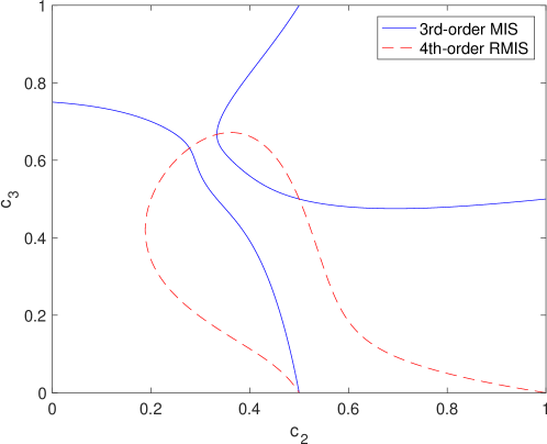
Figure 1: Choices of $c_{2}$ and $c_{3}$ that satisfy the conditions (B) and (52). Values of $c_{2}$ and $c_{3}$ not on these curves result in MIS and RMIS methods of 2nd and 3rd order, respectively.

Of these, only two satisfy the MIS criteria that $c_{2}\leq c_{3}$:

$$(c_{2},c_{3}) =\left(\frac{1}{3},\frac{2}{3}\right),$$ (36)

$$(c_{2},c_{3}) =\left(\frac{2502984374488603}{9007199254740992},\frac{2843567935040037}{4503599627370496}\right)$$ (37)

$$\approx\left(0.27788708828342423285,0.63139891871345210639\right).$$

The first of these corresponds to the “3/8-Rule” from Kutta’s 1901 paper [40],

$$\begin{array}[]{c|cccc}0&0&0&0&0\\ \frac{1}{3}&\frac{1}{3}&0&0&0\\ \frac{2}{3}&-\frac{1}{3}&1&0&0\\ 1&1&-1&1&0\\ \hline\cr&\frac{1}{8}&\frac{3}{8}&\frac{3}{8}&\frac{1}{8}\end{array}$$ (38)

Both due to its historical elegance, as well as its equally-spaced abcissae $c_{i}$, we use this base method for $T_{O}$ in our numerical results.

2.2 RMIS example methods

For numerical testing, we examine methods wherein the inner table $T_{I}$ corresponds to a subcycled version (using approximately $m/s^{O}$ substeps) of the outer table $T_{O}$. This “telescopic” approach facilitates further recursion to support problems with three or more rates; however, that is not studied in this work. We note that due to the patterned structure of both the MIS and RMIS methods, these subcycled algorithms may be implemented more efficiently than a generic GARK scheme having $ms$ fast and $s$ slow stages.

For these methods, we utilize $T_{O}$ as either the four-stage 3/8-Rule (38) above, or the three-stage “KW3” table,

$$\begin{array}[]{c|ccc}0&0&0&0\\ \frac{1}{3}&\frac{1}{3}&0&0\\ \frac{3}{4}&-\frac{3}{16}&\frac{15}{16}&0\\ \hline\cr&\frac{1}{6}&\frac{3}{10}&\frac{8}{15}\\ \end{array}$$ (39)

that satisfies the 3rd-order MIS condition (24). We note that this latter table is frequently used for MIS methods in the literature [1, 5, 7, 8]; moreover, in previous tests of a wide range of multirate methods, we found this combination to be the most efficient (smallest error with least computational cost).

To be more precise regarding how we form $T_{I}$ from these two choices of $T_{O}$ to enable subcycling, we elaborate on the case of a time-scale separation factor $m=100$. Schlegel suggested using $n_{i}=\left\lceil m\left(c^{O}_{i}-c^{O}_{i+1}\right)\right\rceil$ to measure the appropriate number of subcycles for each subcycling period [3]. We used this measure as a guide when selecting $m$ in our methods, although we determined that our method comparisons would be fairest if the ratio of fast function evaluations to slow function evaluations was held approximately constant.

The 3/8-Rule (38) has four evenly-spaced abcissae with final $c^{O}_{s^{O}}=1$. Hence its multirate implementation requires only three subcycling periods, and so we form $T_{I}$ using 34 subcycles of the $T_{O}$ table. The KW3 method has only three abcissae, but $c^{O}_{s^{O}}=\frac{3}{4}<1$, so although it has one fewer stage than the 3/8-Rule, it requires the same number of subcycling periods. Moreover, since these abcissae are unevenly spaced, we could choose between using either different $A^{I}$ per outer stage (to attempt nearly-identical substep sizes) or using a single $A^{I}$ for each outer stage, mapped to the largest subcycling interval. Choosing the latter approach for simplicity, we form $T_{I}$ using 35 subcycles of $T_{O}$. This is a compromise between using the largest subcycling interval for substep sizes and making the work of fast functions vs slow functions comparable.

This gives us the multirate methods:

• “RMIS-3/8”: this is our proposed RMIS method using $T_{O}$ given by (38) that satisfies both the 4th-order condition (25) and the 3rd-order condition (24) – the method should be $\mathcal{O}(h^{4})$ accurate;

• “RMIS-KW3”: this is our proposed RMIS method using $T_{O}$ given by (39) that satisfies (24) but does not satisfy (25) – the method should be $\mathcal{O}(h^{3})$ accurate.

2.3 Optimized method

To further explore the preceding theoretical results, we also consider an “unstructured” form of ${\mathbf{b}}^{\left\{f\right\}}\in\mathbb{R}^{s^{f}}$, where these coefficients are chosen to directly satisfy the equations (26)-(33). Here, since we do not enforce any particular structure on these coefficients, we must consider a fixed time scale separation, $m$ (or equivalently $s^{f}$), here chosen to be $m=100$. As with the RMIS methods above, we choose $T_{I}$ as a subcycled version of $T_{O}$, which we again choose to be the 3/8-Rule, resulting in $s^{f}=408$. Since this allows significantly more coefficients than the number of fourth order condition equations, we use the remaining degrees of freedom in this under-determined system to minimize the two-norm of the residual of all the fifth-order conditions. To solve this minimization problem, we used MATLAB’s fminsearch algorithm, which is based on a simplex search method [41]. Under this approach, we arrive at the multirate method “Opt-3/8,” which should be $\mathcal{O}(h^{4})$ accurate.

2.4 Method Comparison

In the sections that follow, we examine the linear stability, and assess the attainable order of accuracy, for both the proposed RMIS and MIS algorithms. In the ensuing sections we therefore compare the 3 newly developed multirate methods listed above with 2 existing multirate methods:

• “MIS-3/8”: this is the MIS method using $T_{O}$ given by (38) – the resulting method should be $\mathcal{O}(h^{3})$ accurate;

• “MIS-KW3”: this is the MIS method using $T_{O}$ given by (39) – the resulting method should be $\mathcal{O}(h^{3})$ accurate.

We note that although we have suggested an embedding of MIS within RMIS (i.e., MIS-3/8 within RMIS-3/8), optimal approaches for time-step adaptivity (that vary both $h$ and $m$) are not within the scope of this manuscript and are left for future work. We therefore explore each of the above methods using fixed time-step sizes $h$.

3 RMIS Implementation and Memory Considerations

A crucial aspect for the success of multirate methods is their ability to be implemented in both a computationally and memory-efficient manner. First, we recall the formulas (7), corresponding to the generic implementation of a 2-component GARK method:

$${k}^{\left\{{f}\right\}}_{j} =y_{n}+h\sum_{l=1}^{s^{\{f\}}}{a}^{\left\{{f,f}\right\}}_{j,l}f^{\{f\}}\left({k}^{\left\{{f}\right\}}_{l}\right)+h\sum_{l=1}^{s^{\{s\}}}{a}^{\left\{{f,s}\right\}}_{j,l}f^{\{s\}}\left({k}^{\left\{{s}\right\}}_{l}\right),$$

$${k}^{\left\{{s}\right\}}_{i} =\mathbf{y}_{n}+h\sum_{l=1}^{s^{\{f\}}}{a}^{\left\{{s,f}\right\}}_{i,l}f^{\{f\}}\left({k}^{\left\{{f}\right\}}_{l}\right)+h\sum_{l=1}^{s^{\{s\}}}{a}^{\left\{{s,s}\right\}}_{i,l}f^{\{s\}}\left({k}^{\left\{{s}\right\}}_{l}\right),$$

$$y_{n+1} =y_{n}+h\sum_{l=1}^{s^{\{f\}}}{b}^{\left\{{f}\right\}}_{l}f^{\{f\}}\left({k}^{\left\{{f}\right\}}_{l}\right)+h\sum_{l=1}^{s^{\{s\}}}{b}^{\left\{{s}\right\}}_{l}f^{\{s\}}\left({k}^{\left\{{s}\right\}}_{l}\right),$$

where $i=1,\dots,s^{\{s\}}$ and $j=1,\dots,s^{\{f\}}$. We introduce additional notation to better focus on the case where subcycling is employed in the inner method $T_{I}$. Subcycling suggests a natural set of internal divided units, that can be characterized by the block-rows of ${\mathbf{A}}^{\left\{f,f\right\}}$ and ${\mathbf{A}}^{\left\{f,s\right\}}$ which correspond to each fast substep. To this end, we define the fast stage abcissae in vector form as

$${\mathbf{c}}^{\left\{f\right\}}=\begin{bmatrix}{\mathbf{c}}^{\left\{f,1\right\}}\\ \vdots\\ {\mathbf{c}}^{\left\{f,s^{O}\right\}}\end{bmatrix},\quad\text{where}\quad{\mathbf{c}}^{\left\{f,i\right\}}=\begin{bmatrix}c_{i-1}^{O}+c_{1}^{I}\left(c_{i}^{O}-c_{i-1}^{O}\right)\\ \vdots\\ c_{i-1}^{O}+c_{s^{I}}^{I}\left(c_{i}^{O}-c_{i-1}^{O}\right)\end{bmatrix}.$$

We make row block indices corresponding to these stage vectors, which correspond to the smallest unit step; the column block indices delineate the same organization for how ${\mathbf{b}}^{\left\{f\right\}}$ is used. This then gives us ${\mathbf{A}}^{\left\{f,f,i,j\right\}}$ and ${\mathbf{A}}^{\left\{f,s,i\right\}}$, where $i$ denotes the block-row, and $j$ denotes the block-column. This also allows ${{k}^{\left\{f\right\}}}$ to be represented in terms of block-row units, ${{k}^{\left\{f\right\}}}={\begin{bmatrix}{{{k}^{\left\{f,1\right\}}}}^{\intercal}&\cdots&{{{k}^{\left\{f,s^{O}\right\}}}}^{\intercal}\end{bmatrix}}^{\intercal}$, where ${k}^{\left\{{f,i}\right\}}_{j}$ is the $j$th fast stage vector for the $i$th block. Since we have assumed the first stage of $T_{I}$ is explicit, then the coefficients ${a}^{\left\{{f,f,i,j}\right\}}_{1,q}={a}^{\left\{{s,f,j}\right\}}_{i,q}$ and $a_{1,l}^{\{f,s,i\}}=a_{i,l}^{\{s,s\}}$. We leverage this structure by specifically defining ${\hat{k}}^{\left\{{f,i}\right\}}_{1}$ (the fast stage solution from the $i$th block) to be ${k}^{\left\{{f,i}\right\}}_{1}$ with the slow coupling portion removed,

$${\hat{k}}^{\left\{{f,i}\right\}}_{1}={k}^{\left\{{f,i}\right\}}_{1}-h\sum_{l=1}^{s^{\{s\}}}a_{1,l}^{\{f,s,i\}}f^{\{s\}}\left({k}^{\left\{{s}\right\}}_{l}\right).$$

This portion of the stage solution is then used to accumulate an initial condition for ${k}^{\left\{{f,i}\right\}}_{p}$ for $p=2,\dots,s^{I}$, and to calculate the next initial condition ${\hat{k}}^{\left\{{f,i+1}\right\}}_{1}$. Finally, this accumulated initial condition ${k}^{\left\{{f,s^{O}}\right\}}_{1}$ can be used with the remaining ${k}^{\left\{{f,s^{O}}\right\}}_{p}$ stages to form the fast portion of an embedded MIS solution method (if desired). The formulas for these are as follows:

$${\hat{k}}^{\left\{{f,1}\right\}}_{1} =y_{n}$$

$${k}^{\left\{{f,i}\right\}}_{1} ={\hat{k}}^{\left\{{f,i}\right\}}_{1}+h\sum_{l=1}^{s^{\{s\}}}a_{1,l}^{\{f,s,i\}}f^{\{s\}}\left({k}^{\left\{{s}\right\}}_{l}\right)$$

$${\hat{k}}^{\left\{{f,i}\right\}}_{1} =\sum_{p=1}^{i-1}{k}^{\left\{{f,i}\right\}}_{1}+h\sum_{l=1}^{s^{I}}b_{l}^{I}\left(c_{i}^{O}-c_{i-1}^{O}\right)f^{\{f\}}\left({k}^{\left\{{f,i-1}\right\}}_{l}\right)$$

$${k}^{\left\{{f,i}\right\}}_{j} ={\hat{k}}^{\left\{{f,i}\right\}}_{1}+h\sum_{l=1}^{j-1}a_{jl}^{\{f,f,i,i\}}f^{\{f\}}\left({k}^{\left\{{f}\right\}}_{l}\right)+h\sum_{l=1}^{s^{\{s\}}}a_{jl}^{\{f,s,i\}}f^{\{s\}}\left({k}^{\left\{{s}\right\}}_{l}\right)$$

$${k}^{\left\{{s}\right\}}_{i} ={\hat{k}}^{\left\{{f,i}\right\}}_{1}+h\sum_{l=1}^{i-1}a_{il}^{\{s,s\}}f^{\{s\}}\left({k}^{\left\{{s}\right\}}_{l}\right)$$

$$\tilde{y}_{n+1} ={k}^{\left\{{f,s^{O}}\right\}}_{1}+h\sum_{l=1}^{s^{I}}b_{l}^{I}\left(1-c_{s^{O}}^{O}\right)f^{\{f\}}\left({k}^{\left\{{f,s^{O}}\right\}}_{l}\right)+h\sum_{l=1}^{s^{\{s\}}}b_{l}^{\{s\}}f^{\{s\}}\left({k}^{\left\{{s}\right\}}_{l}\right)$$

$$y_{n+1} =y_{n}+h\sum_{l=1}^{s^{\{f\}}}b_{l}^{\{f\}}f^{\{f\}}\left({k}^{\left\{{f}\right\}}_{l}\right)+h\sum_{l=1}^{s^{\{s\}}}b_{l}^{\{s\}}f^{\{s\}}\left({k}^{\left\{{s}\right\}}_{l}\right)$$

where the final step solution $y_{n+1}$ is built up by successive fast substeps, and where the slow information is updated as needed.

To remove duplicate function calls, we use temporary vectors for the contributions of our base methods to the solution. In particular, while computing the update formulas for ${k}^{\left\{{f,i}\right\}}_{j}$ and ${k}^{\left\{{s}\right\}}_{i}$, we store ${k}^{\left\{{f,i}\right\}}_{1}$, the $s^{I}$ fast function vectors ${\phi}^{\left\{{f,i}\right\}}_{l}=f^{\{f\}}\left({k}^{\left\{{f,i}\right\}}_{l}\right)$, and the $s^{O}$ slow function vectors ${\phi}^{\left\{{s}\right\}}_{l}=f^{\{s\}}\left({k}^{\left\{{s}\right\}}_{l}\right)$. These provide sufficient storage to compute the embedded MIS solution $\tilde{y}_{n+1}$ without additional function calls. Moreover, to compute the RMIS solution $y_{n+1}$, we must additionally store $y_{n+1}$ and the vector of coefficients ${\mathbf{b}}^{\left\{f\right\}}$, if these are unique or unstructured. We may condense storage slightly so that we need only retain $s^{I}+s^{O}+2$ vectors the size of our solution $y$, by overwriting ${{\phi}^{\left\{f,i\right\}}}$ with ${{\phi}^{\left\{f,i+1\right\}}}$ after the $i$th fast substep has completed, and ${{\phi}^{\left\{f,i\right\}}}$ has been used to generate the initial condition ${\hat{k}}^{\left\{{f,i+1}\right\}}_{1}$ for the fast substep $(i+1)$. When using subcycling for the fast steps, we overwrite ${{\phi}^{\left\{f,i\right\}}}$ after each subcycled fast substep has completed, and ${{\phi}^{\left\{f,i\right\}}}$ has been used to update the temporary initial condition ${\hat{k}}^{\left\{{f,i}\right\}}_{1}$ for the next subcycled fast substep.

When considering only the structured form of MIS and RMIS methods, further optimizations may be used since the overall time step may be broken apart into a sequence of “fast” subproblems, and where each subproblem only receives forcing terms from the slow stage right-hand side functions $f^{\{s\}}$. To this end, we have provided an open-source MATLAB implementation of this structured form for both RMIS and MIS methods [42]. We note that this repository does not include an implementation of the “Opt-3/8” method described previously in Section 2.3, as that requires an unstructured ${\mathbf{b}}^{\left\{f\right\}}$; however, in this repository we also include a file opt38_coeffs.m that contains these ${\mathbf{b}}^{\left\{f\right\}}$ coefficients for interested readers.

4 RMIS and MIS linear stability analysis

In their paper introducing GARK methods [10], Sandu and Günther analyze linear stability using a modification of the standard Dahlquist test problem,

$$y^{\prime}=\sum_{m=1}^{N}\lambda^{\{m\}}y,\qquad y(0)=1,$$

which in the current context of a two-rate problem becomes

$$y^{\prime}=\lambda^{\{f\}}y+\lambda^{\{s\}}y,\qquad y(0)=1,$$

and where they assume that the real parts of both $\lambda^{\{f\}}$ and $\lambda^{\{s\}}$ must be negative. While that approach yields elegant definitions of the resulting GARK stability regions, we prefer an approach for multirate linear stability analysis that was first proposed by Kværnø [23] in 2000, has subsequently been used by a variety of authors [29, 43, 44, 45, 46], and which we summarize here. In this approach, one instead considers the partitioned test problem

$$\begin{bmatrix}y_{f}^{\prime}\\ y_{s}^{\prime}\end{bmatrix}=\begin{bmatrix}g_{11}&g_{12}\\ g_{21}&g_{22}\end{bmatrix}\begin{bmatrix}y_{f}\\ y_{s}\end{bmatrix},\qquad\begin{bmatrix}y_{f}(0)\\ y_{s}(0)\end{bmatrix}=\begin{bmatrix}1\\ 1\end{bmatrix}$$ (40)

$$\Leftrightarrow\quad$$

$$y^{\prime}=Gy,\qquad y(0)=\mathbbm{1}^{\{2\}}.$$

Here, $y_{f}$ and $y_{s}$ correspond to the fast and slow variables, respectively, with a resulting splitting of the right-hand side into fast and slow components as shown in (2). The benefit of this approach is that unlike the purely additive scalar version, this directly allows analysis of stability as a function of the strength of fast/slow coupling in the problem, and does not require simultaneous diagonalizability of the Jacobians of $f^{\left\{s\right\}}$ and $f^{\left\{f\right\}}$ to derive the linear stability problem. Defining the matrix $Z=hG$, stability is ascertained by first determining the amplification matrix $S(Z)$ for one step of the numerical method, i.e.

$$y_{n+1}=S(Z)\,y_{n},\quad\text{where}\quad S(Z)=\begin{bmatrix}s_{11}(Z)&s_{12}(Z)\\ s_{21}(Z)&s_{22}(Z)\end{bmatrix}.$$

The multirate method is then linearly stable if the eigenvalues of $S$ have magnitude less than $1$ for a given step size $Z=hG$.

While more complex than standard IVP linear stability regions, the number of independent parameters may be reduced from five ($h,g_{1,1},g_{1,2},g_{2,1},g_{2,2}$) to a more manageable three [43, 44, 46]. First, the eigenvalues of $G$ have negative real part if $g_{11},g_{22}<0$ and $\beta=\frac{g_{12}g_{21}}{g_{11}g_{22}}<1$, where here $\beta$ is a measure of the off-diagonal coupling strength of the problem. Under this assumption, the eigenvalues of $S(Z)$ depend on only three parameters:

$$\kappa =\frac{g_{22}}{g_{11}}>0,$$ (41)

$$\xi =\frac{hg_{11}}{1-hg_{11}}\in\left(-1,0\right),$$ (42)

$$\eta =\frac{\beta}{2-\beta}\in(-1,1).$$ (43)

Here, $\kappa$ encodes the time-scale separation of the problem, $\xi$ encodes the stiffness of the fast time scale (as $hg_{11}$ goes from $0\to-\infty$, $\xi$ moves from $0\to-1$), and $\eta$ encodes the strength of coupling (no coupling at $\eta=0$, increased coupling as $|\eta|\to 1$, coupling-dominant as $\eta\to-1$). The stability of a multirate method may then be visualized using snapshots of the $(\xi,\eta)$ stability regions for fixed values of $\kappa$.

In the stability region plots that follow, we match the problem and method time-scale separation values, i.e. $\kappa=m$. We then create linearly-spaced arrays of 100 $\xi$ values in $(-1,0)$ and 200 $\eta$ values in $(-1,1)$. For each of the 20000 resulting $(\xi_{i},\eta_{j})$ combinations, we compute the eigenvalues of $S(Z)$ to determine stability, and mark the stable regions in yellow and unstable regions in blue.

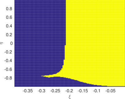
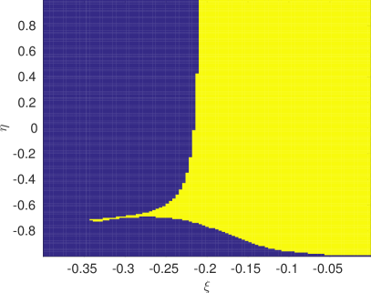
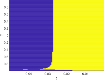
Figure 2: Linear stability plots for the RMIS-3/8 (left) and MIS-3/8 (right) methods at time-scale separation values $\kappa=m=10$ (top) and $\kappa=m=100$ (bottom), showing the stable region in yellow. Note that the $\kappa=100$ plots are zoomed in to a smaller $\xi$ region than the $\kappa=10$ plots.

In Figure 2 we plot the stability regions for the RMIS-3/8 and MIS-3/8 methods for $\kappa=m=\{10,100\}$. We see that the stability regions for both methods are similar: for weakly coupled fast and slow time scales, these indicate stability for $\xi$ values close to zero and instability for $\xi$ close to -1, as would be expected for any explicit method. Additionally, both exhibit a region of increased stability for problems with stronger fast/slow coupling, followed by complete instability as $\eta\to-1$ (where the coupling terms become infinitely large). Comparing the plots of $\kappa=10$ versus 100, we see that the region of increased stability shifts toward stronger fast/slow coupling as the problem time-scale separation increases. Lastly, as expected for explicit methods, the maximum stable step size shrinks as the fast time scale decreases.

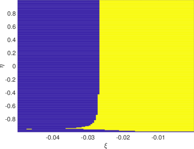
Figure 3: Linear stability plots for the RMIS (left) and MIS (right) methods based on the alternate possibility for $T_{O}$, at time-scale separation factors $\kappa=m=10$ (top) and $\kappa=m=100$ (bottom), showing the stable region in yellow. Note that the $\kappa=100$ plots are zoomed in to a smaller $\xi$ region than the $\kappa=10$ plots.

To see whether these stability properties translate to other RMIS and MIS methods (as opposed to only the ones based on the 3/8-Rule), we additionally examine the linear stability of the RMIS and MIS methods that use the other 4-stage base method $T_{0}$ satisfying the 3rd-order MIS and 4th-order RMIS conditions, given by the intersection point (37) from Figure 1. These plots are shown in Figure 3. While the precise shapes of these stability regions have changed slightly from those in Figure 2, the properties observed above are indeed retained for this alternate base method.

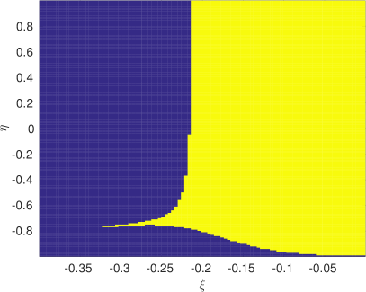
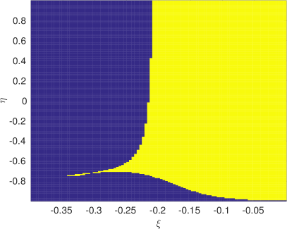
Figure 4: Linear stability plots for the RMIS (left) and MIS (right) methods having ‘maximal’ stability regions for time-scale separation factor $\kappa=m=10$, showing the stable region in yellow.

As a final stability comparison between MIS and RMIS methods, we investigated the following question: given that there exist one-parameter families of 3rd-order MIS methods and 4th-order RMIS methods (as seen in Figure 1), can we find the MIS and RMIS methods with ‘largest’ linear stability regions, and how would these compare against one another? To this end, we tested 100 base methods along this one-parameter family for each method, and selected the one with largest stability region (maximal area of the yellow region). The results of this investigation for $\kappa=m=10$ are shown in Figure 4. We again note the similar stability regions as before, showing slight variations in the stability boundaries but the same overall shapes.

Based on the results shown in this section, we conclude that the proposed RMIS methods suffer no deterioration in stability as compared with their MIS ‘cousins’.

5 Convergence and Efficiency Tests

In this section we provide numerical results to verify the analytical order of the proposed RMIS methods and compare their efficiency against the MIS methods of [1]. To that end, we consider three standard multirate tests, corresponding to the inverter-chain problem [19, 20, 22, 29], a linear multirate problem with strong fast/slow coupling from Kuhn and Lang [46], and the well-known brusselator problem. For each problem we either compare against the analytical solution or a high-accuracy reference solution. These reference solutions were generated by using the $12$th order Gauss implicit Runge-Kutta method, using fixed time-steps which are $4$ times smaller than the smallest $h$ value tested for our multirate methods.

We measure solution error in each test by computing the root-mean-square error over all solution components and over all time steps $t_{n}=t_{0}+hn$,

$$\mathtt{RMSerror}=\left(\frac{1}{MN}\sum_{n=1}^{M}\left\|y_{n,h}-y_{n,ref}\right\|_{2}^{2}\right)^{1/2},$$ (44)

where $y_{n,h}$ and $y_{n,ref}$ are our computed and reference solutions in $\mathbb{R}^{n}$ at $t_{n}$, respectively, $\|\cdot\|_{2}$ is the standard vector 2-norm, and $M=(t_{F}-t_{0})/h$ is the total number of overall time steps of size $h$ taken i n each run over $t\in\left[t_{0},t_{F}\right]$. For each test, we present both plots of $\mathtt{RMSerror}$ versus $h$, as well as tables of the observed numerical order. These observed orders are computed using a least-squares fit to these data where outliers are ignored, i.e., the numerical orders of convergence only include data where $10^{-9}\leq\mathtt{RMSerror}\leq 1$.

To assess the efficiency of each method, we utilize standard error-versus-cost plots. Since these simulations were performed in MATLAB, where timings can provide rather poor predictions of runtimes for true HPC applications, in these tests we measure cost by counting the total number of ODE right-hand side function calls. For the subcycled and telescopic RMIS and MIS methods examined here, this may be easily calculated as

$$\mathtt{TotalFunctionCalls}=s^{O}+s^{I}\sum_{i=1}^{s^{O}}n_{i},$$ (45)

where $n_{i}$ is the number of fast step subcycles required per slow stage $i$. In the context of our five methods (Opt-3/8, RMIS-3/8, RMIS-KW3, MIS-3/8, and MIS-KW3), we may examine this accounting for a time-scale separation of $m=100$. Since the methods based on the 3/8-Rule perform 34 subcycles per outer stage, and the methods based on KW3 perform 35 subcycles per outer stage, the total number of right-hand side function calls per outer step are $4+4(34+34+34)=412$ and $3+3(35+35+35)=318$. These per-step costs are summarized in Table 1.

Method Efficiency	$s^{O}$	$s^{f}/s^{s}$	$s^{O}\left(1+\sum_{i=1}^{s^{O}}n_{i}\right)$
Opt-3/8	4	102	412
RMIS-3/8	4	102	412
RMIS-KW3	3	105	318
MIS-3/8	4	102	412
MIS-KW3	3	105	318

Table 1: Per-step method costs: the choice of $T_{O}$ determines the number of stages $(s^{O})$ and subcycles per outer stage $(n_{i})$, resulting in slight differences in the ratio of fast stages to slow stages in each method.

With these data, for each test we plot $\mathtt{RMSerror}$ versus $\mathtt{TotalFunctionCalls}$; “efficient” methods correspond to curves that are nearest the bottom-left corner.

5.1 Inverter-chain

The inverter-chain problem is a partitioned multirate ODE system that models a chain of MOSFET inverters, which has been used for testing multirate ODE solvers throughout the literature [1, 20, 22, 29, 43, 45, 47, 48, 49, 50, 51]. The form of the model that we examine is primarily based on the version used by Kværnø and Rentrop [19], although we utilize an additional scaling term as used in [20, 29]. The mathematical model is given by the system of ODEs for $y(t)\in\mathbb{R}^{n_{I}}$, $0\leq t\leq 7$:

$$y_{k}^{\prime}(t)=y_{op}-y_{k}(t)-\gamma g_{k}(t,y),\quad y_{k}(0)=0,\quad k=1,\ldots,n_{I},$$ (46)

where

$$g_{k}(t,y) =\begin{cases}g(y_{in}(t),y_{1}(t),y_{0}),&k=1\\ g(y_{k-1}(t),y_{k}(t),y_{0}),&1<k\leq n_{I}\end{cases},$$

$$g(y_{G},y_{D},y_{S}) =\left(\max\left(y_{G}-y_{S}-y_{T},0\right)\right)^{2}-\left(\max\left(y_{G}-y_{D}-y_{T},0\right)\right)^{2},$$

where $y_{op}=5$ V, $y_{T}=1$ V, $y_{0}=0$ V, $\gamma$ is the scaling term for tuning the time-scale separation of the problem (we use $\gamma=100$), and $y_{in}(t)$ is the forcing function,

$$y_{in}(t)=\begin{cases}0,&0\leq t<5,\\ t-5,&5\leq t\leq 7.\end{cases}$$

We note that $y_{in}(t)$ causes the problem (46) to be non-autonomous. This is easily handled since the MIS and RMIS methods are internally consistent, so we may identify ‘stage times’ $t_{n,l}^{\{q\}}=t_{n}+c^{\{q\}}_{l}h$ that correspond to each stage $k_{l}^{\{q\}}$.

The time scales for these inverters decrease with index, so we partition this so that the first $b$ equations are “fast” and the remainder are “slow”,

$$f^{\left\{f\right\}}(t,y)^{\intercal} =\begin{bmatrix}y_{1}^{\prime}(t)&\cdots&y_{b}^{\prime}(t)&0&\cdots&0\end{bmatrix}$$

$$f^{\left\{s\right\}}(t,y)^{\intercal} =\begin{bmatrix}0&\cdots&0&y_{b+1}^{\prime}(t)&\cdots&y_{n_{I}}^{\prime}(t)\end{bmatrix}.$$

In our tests, we use $n_{I}=100$ total inverters, with the first $b=3$ grouped into $f^{\left\{f\right\}}(t,y)$. We note that in other papers that use a similar setup, the first $b=20$ were chosen as “fast”; however in our tests we found that only 3 were required for our desired multirate time-scale separation factor of $m=100$. In Figure 5 we show the solutions for this problem, as well as a zoom-in of the initial departure of the fast inverters from the larger group. In our tests we found that accuracy in these initial departures proved crucial for overall solution accuracy.

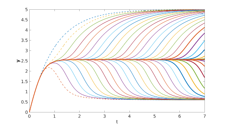
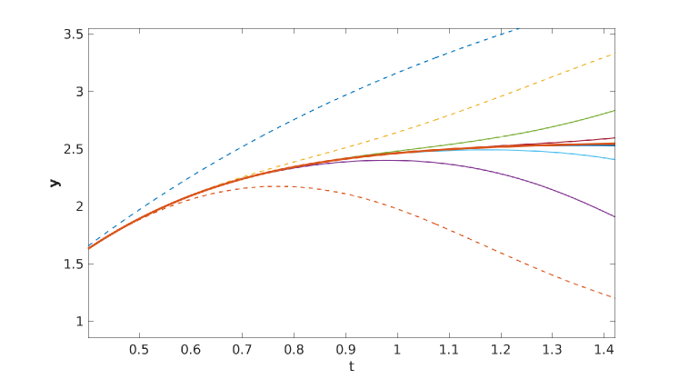
Figure 5: Solutions for the inverter chain problem with $n_{I}=100$: Dotted lines represent the fast components, i.e. $y_{1}$ is the blue dotted curve at the top-left and $y_{100}$ remains at the value 2.5 at the final time. At bottom is a zoom-in of the initial departure of fast components, indicating that even small differences in the initial integration solution may result in disparate overall solution values.

In the left portion of Figure 6 we plot $\mathtt{RMSerror}$ versus step size $h$ for each of the five methods tested. We highlight a few observations in these results. First, all methods demonstrate convergence as $h\to 0$ to a point, beyond which convergence stagnates. This stagnation point is below $10^{-9}$ for all but the Opt-3/8 method, that stagnates slightly earlier at around $10^{-8}$, indicating a reference solution accurate to approximately $10^{-9}$ for this test. We hypothesize that the Opt-3/8 method is more susceptible to accumulation of floating-point round-off than the other methods, since unlike the others that are defined by a structured pattern of small-valued coefficients, Opt-3/8 has more widely-varying coefficients ${\mathbf{b}}^{\left\{f\right\}}_{i}\in\left[-5.5\times 10^{4},1.2\times 10^{5}\right]$. Second, both the RMIS-3/8 and Opt-3/8 methods show faster rates of convergence than the other methods; unfortunately, the stagnation of Opt-3/8 halts this fast convergence somewhat early, but RMIS-3/8 shows consistently fast convergence until below the reference solution accuracy. The best-fit orders of convergence for the results from this figure are: 1.74 (Opt-3/8), 4.07 (RMIS-3/8), 2.93 (RMIS-KW3), 2.98 (MIS-3/8) and 2.98 (MIS-KW3). We note that all show their expected rates of convergence except for Opt-3/8, which is likely due to its larger error floor, since prior to that point it is converging at least as rapidly as the 3rd-order methods.

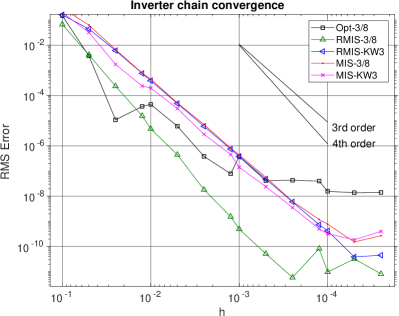
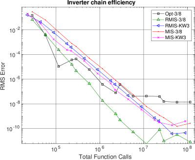
Figure 6: Convergence (left) and efficiency (right) for the inverter chain problem: the convergence results are consistent with expectations for all methods except Opt-3/8, where the early flattening of the error is likely due to increased sensitivity to floating-point round-off. Here, the most efficient methods for larger error values are RMIS-3/8 and Opt-3/8, while for smaller errors RMIS-3/8 is the clear winner; all other methods perform comparably well.

Accuracy alone provides only an incomplete picture of performance, since the methods using the 3/8-Rule require 25% more function calls per step than those using KW3. To this end, in the right portion of Figure 6 we also plot the $\mathtt{RMSerror}$ versus $\mathtt{TotalFunctionCalls}$ for each of the five methods. Although the blue and magenta curves for the KW3-based methods indeed shift further to the left in relation to the other methods, RMIS-3/8 is still the most efficient of all the methods at nearly all error values, and is only outperformed by Opt-3/8 for relatively loose error values (above $\sim\!10^{-4}$). The efficiency benefit of RMIS-3/8 is most notable for errors below $\sim\!10^{-8}$, where it requires approximately 10 times less work than the other methods.

5.2 Strongly-coupled Linear Test

As a second test, we use a linear ODE system with strong fast/slow coupling that was used by Kuhn and Lang in their studies of multirate stability [46]; variants of this problem have been used by a variety of authors in testing multirate algorithms [23, 29, 46]. Our motivation for this test is to more rigorously explore accuracy and efficiency of the RMIS and MIS algorithms in the face of strongly-coupled problems, thereby exercising the coupling matrices ${\mathbf{A}}^{\left\{f,s\right\}}$ and ${\mathbf{A}}^{\left\{s,f\right\}}$, and exploring whether the extreme sparsity of our ${\mathbf{b}}^{\left\{f\right\}}$ in the RMIS algorithm causes trouble for strongly-coupled problems. The ODE system is identical to the partitioned test problem (40) examined in Section 4, where here the system-defining matrix is given by

$$G=\begin{bmatrix}-5&-1900\\ 5&-50\end{bmatrix}$$

and the problem is evolved over the time interval $t\in[0,1]$. The eigenvalues of $G$ are complex conjugates,

$$\lambda=-\frac{55\pm 5i\sqrt{1439}}{2},$$

giving rise to the analytical solution

$$\begin{bmatrix}y_{1}\\ y_{2}\end{bmatrix}=e^{-\frac{55}{2}t}\begin{bmatrix}\cos\left(\frac{5\sqrt{1439}t}{2}\right)-\frac{751}{\sqrt{1439}}\sin\left(\frac{5\sqrt{1439}t}{2}\right)\\ \cos\left(\frac{5\sqrt{1439}t}{2}\right)-\frac{7}{\sqrt{1439}}\sin\left(\frac{5\sqrt{1439}t}{2}\right)\end{bmatrix}.$$

which is shown in Figure 7. The time-scale separation in this problem arises from the strong fast/slow coupling, rendering the ‘sin’ term in $y_{1}$ approximately 100 times stronger than in $y_{2}$, at least until the solutions decay to zero.

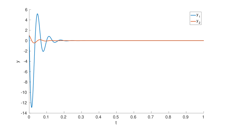
Figure 7: Solutions for the linear test problem: note that the “slow” component $y_{2}$ varies far less than strongly than the “fast” component $y_{1}$.

We cast this problem into additive multirate form by partitioning the right-hand side into fast and slow components,

$$f^{\left\{f\right\}}(y)=\begin{bmatrix}-5&-1900\\ 0&0\end{bmatrix}\begin{bmatrix}y_{1}\\ y_{2}\end{bmatrix}\quad\text{and}\quad f^{\left\{s\right\}}(y)=\begin{bmatrix}0&0\\ 5&-50\end{bmatrix}\begin{bmatrix}y_{1}\\ y_{2}\end{bmatrix}.$$

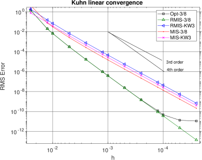
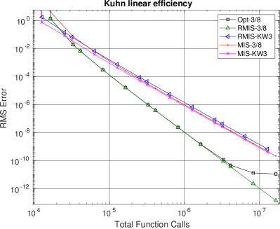
Figure 8: Convergence (left) and efficiency (right) for the linear test problem: the convergence results are consistent with expectations for all methods, and the 4th-order methods show significantly better efficiency than the 3rd-order methods.

In Figure 8 we plot both $\mathtt{RMSerror}$ versus $h$ (left) and $\mathtt{RMSerror}$ versus $\mathtt{TotalFunctionCalls}$ (right). This problem exhibits very straight order of accuracy lines for all methods except Opt-3/8, which begins to level off at approximately $10^{-11}$, again likely due to increased sensitivity to accumulation of floating-point round-off errors. The best-fit convergence orders for these results are: 4.22 (Opt-3/8), 4.22 (RMIS-3/8), 3.09 (RMIS-KW3), 3.18 (MIS-3/8) and 3.09 (MIS-KW3). We do not fully understand the higher-than-expected orders of accuracy for Opt-3/8 and RMIS-3/8, except that since the problem is linear then many of the GARK order conditions are irrelevant. As with the previous problem, the reduced cost per step of the KW3-based methods is insufficient to surpass the efficiency of the 4th-order methods, with Opt-3/8 and RMIS-3/8 demonstrating essentially-identical efficiency for errors larger than $10^{-10}$, and with RMIS-3/8 proving more efficient past that point.

5.3 Brusselator

We consider a system of stiff nonlinear ODEs that captures some of the physical challenges of the brusselator chemical reaction network problem, first described as a 1D PDE by Prigogine in 1967 [52]. More recently this test was used in a multiphysics paper by Estep in 2008, and a general computational multiphysics review paper in 2013 [53, 54]. Our version of the problem is a tunable two-rate initial-value problem represented as a system of three nonlinearly-coupled ODEs,

$$y^{\prime}(t) =f^{\left\{f\right\}}(y)+f^{\left\{s\right\}}(y),\quad 0\leq t\leq 10$$

$$y(0) =\begin{bmatrix}3.9&1.1&2.8\end{bmatrix}^{\intercal}$$

where (47)

$$f^{\left\{f\right\}}(y) =\begin{bmatrix}0\\ 0\\ \frac{b-y_{3}}{\varepsilon}\end{bmatrix}\quad\text{and}\quad f^{\left\{s\right\}}(y)=\begin{bmatrix}a-(y_{3}+1)y_{1}+y_{2}y_{1}^{2}\\ y_{3}y_{1}-y_{2}y_{1}^{2}\\ -y_{3}y_{1}\end{bmatrix},$$

where the parameters are chosen to be $a=1.2$, $b=2.5$, and $\varepsilon=10^{-2}$. As shown in the above partitioning, the fast function $f^{\left\{f\right\}}$ contains only the term which is scaled by $\varepsilon$; the problem time-scale separation is approximately $1/\varepsilon=100$. With this particular setup, the problem exhibits a rapid change in the solution at the start of the simulation for $t<0.2$, with slower variation for the remainder of the time interval, as shown in Figure 9.

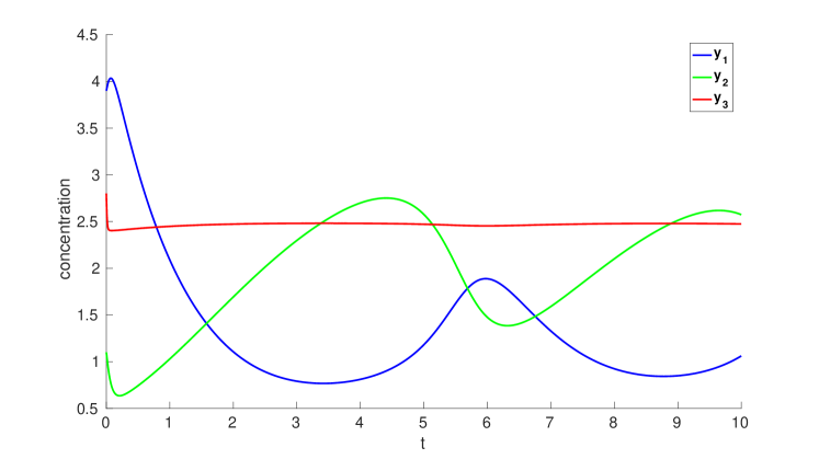
Figure 9: Solutions for the Brusselator test problem (47): note that all components vary rapidly at first and only slowly thereafter.

In the left portion of Figure 10 we plot $\mathtt{RMSerror}$ versus $h$, and on the right we plot $\mathtt{RMSerror}$ versus $\mathtt{TotalFunctionCalls}$. These plots show perhaps the most interesting results of the three tests. Focusing first on the convergence plots we note an intersection point in the curves, showing that the optimal choice of method can depend more intimately on the desired solution error. Beginning at the large-error end, we see that the MIS-KW3 method has smallest error at the largest tested step sizes, although those errors are not significantly different than those for MIS-3/8 or RMIS-3/8. At smaller $h$ and smaller error values, the increased accuracy of RMIS-3/8 and Opt-3/8 appear, rapidly achieving errors $\sim\!100$ times smaller than the 3rd-order methods at step sizes $\sim\!2\times 10^{-3}$. Convergence of all methods stagnates at approximately $10^{-9}$, clearly indicating the accuracy of our reference solution. The corresponding best-fit estimates of the convergence orders for these results are: 5.83 (Opt-3/8), 4.16 (RMIS-3/8), 3.30 (RMIS-KW3), 3.28 (MIS-3/8) and 3.02 (MIS-KW3). We point out the ‘superconvergent’ behavior of Opt-3/8, which suggests that the optimization successfully minimized the dominant 5th-order error terms of relevance to this problem. The other methods have an observed numerical order of accuracy consistent with our theoretical expectations.

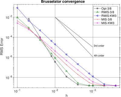
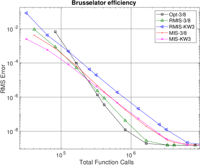
Figure 10: The optimized method and the RMIS seem to do best. Method efficiency for this problem is dependent on both the order of accuracy and on the constant multiplier on the error terms

When examining the efficiency plot at the right of Figure 10, we observe that the decreased cost per step of the KW3-based methods shift those results to the left; making MIS-KW3 the clear winner for larger error values. However, at error values below $\sim\!10^{-5}$, the higher order methods begin to outperform the lower order methods, with Opt-3/8 the most efficient, followed by RMIS-3/8.

6 Conclusions

In this work, we propose a variation of the existing MIS multirate methods [1, 2, 3, 4, 5, 6, 7, 8]. Both the original MIS methods, as well as our extensions, demonstrate a number of very attractive properties for multirate integration. These methods are telescopic, allowing for recursion to any number of problem time scales, allow subcycling of the fast method within the slow, and are highly flexible in that they allow for varying the time-scale separation of the method ($m$) between steps. Finally, when constructed using inner and outer Runge–Kutta methods, $T_{I}$ and $T_{O}$, of at least third order, MIS methods are at worst second order accurate and achieve third order when $T_{O}$ satisfies the auxiliary condition (24).

Recent theory by Sandu and Günther complements these MIS methods nicely. Specifically, they have proposed a general formulation for analyzing a wide range of Runge-Kutta-like methods, named “Generalized-structure Additive Runge-Kutta” (GARK) methods [10], that lays a strong theoretical foundation for understanding and extending MIS methods. More beneficial, however, is their subsequent work that directly analyzed MIS methods using their GARK framework [13], opening the door for subsequent extensions to this analysis.

In this context, we propose a new multirate algorithm which we name “relaxed multirate infinitesimal step” (RMIS), due to a relaxation from the MIS approach on how the fast stage solutions are combined to construct the overall multirate step solution (i.e., the coefficients ${\mathbf{b}}^{\left\{f\right\}}$). This simple change, while leaving the remainder of the MIS approach intact (i.e., the algorithmic approach as well as the coefficients ${\mathbf{A}}^{\left\{f,f\right\}}$, ${\mathbf{A}}^{\left\{f,s\right\}}$, ${\mathbf{A}}^{\left\{s,f\right\}}$, ${\mathbf{A}}^{\left\{s,s\right\}}$ and ${\mathbf{b}}^{\left\{s\right\}}$), allows for a number of remarkable extensions to their work. First, we are able to construct up to fourth order, and at least third order, multirate methods with comparable stability and improved efficiency to MIS methods, where the determining factors for order four are: $T_{I}$ must be at least third order and have explicit first stage; $T_{O}$ must be explicit, at least fourth order, and must satisfy the condition (25). A key component of this analysis is our result from Lemma 1, where we show that due to our selection of the coefficients ${\mathbf{b}}^{\left\{f\right\}}$, the fast order conditions are equivalent to the slow conditions, so one only needs to prove half of the conditions to guarantee overall order of accuracy. These new methods show nearly identical stability properties, and retain all of the above “attractive properties” described above for MIS methods (telescopic, subcycling-ready, flexible to adjusting $m$). In addition, since MIS and RMIS only differ in their selection of the ${\mathbf{b}}^{\left\{f\right\}}$ coefficients, then it is straightforward to define MIS as an embedding within an RMIS method.

In addition to providing detailed proof of the fourth order conditions for the RMIS algorithm, and comparison of the linear stability between MIS and RMIS methods, we provide numerical comparisons of the performance of multiple RMIS and MIS methods on three standard multirate test problems in Section 5. These problems include the standard “inverter-chain” system of nonlinearly coupled ODEs, a linear multirate problem with strong fast/slow coupling, and the standard “brusselator” stiff nonlinear ODE system. Through these experiments, we note that our theoretical expectations regarding the order of accuracy for each method are borne out in the results for each problem, namely that the RMIS methods satisfying (25) exhibit fourth order convergence while those that do not are only third order accurate, and that the MIS methods are at best third order accurate (even when using higher-order base methods). As a result, due to its consistently strong performance (stability, error and efficiency), the proposed RMIS-3/8 method is a clear contribution to the ever-growing ‘stable’ of multirate methods, particularly when highly-accurate solutions are desired.

Although at the time when we performed this work no other fourth-order multirate methods existed, the subsequent release of preprints by Sandu and collaborators demonstrating alternate approaches for fourth-order multirate methods warrants discussion here. Each of the available fourth-order methods (MrGARK [33], MRI-GARK [36], and RMIS), follow distinct approaches for obtaining higher order. The MrGARK methods pre-select the tables ${\mathbf{A}}^{\left\{f,f\right\}}$ and ${\mathbf{A}}^{\left\{s,s\right\}}$ and the value $m$, and then construct fast/slow coupling coefficients ${\mathbf{A}}^{\left\{f,s\right\}}$ and ${\mathbf{A}}^{\left\{s,f\right\}}$ to satisfy requisite coupling conditions. The MRI-GARK and RMIS methods, on the other hand, define a set of modified “fast” initial value problems using the slow right-hand side function values, $f^{\left\{s\right\}}$, allowing for significantly more flexibility in the choice of integrator for the fast time scale. However, these approaches differ in two fundamental areas. First, the fast time-scale IVP modification in RMIS is simpler than that for MRI-GARK, requiring storage of only a single vector to encode the slow-to-fast source terms, as opposed to a vector-valued time-dependent function. While perhaps not as costly as other components of the solves, this reduced memory and computation footprint hints that RMIS may be more efficient per-step than MRI-GARK. Second, the approach for obtaining fourth order differs dramatically between these methods; RMIS methods will automatically obtain this accuracy through proper selection of the outer Butcher table, $T_{O}$ – as shown in Figure 1 there are infinitely many options in this regard. MRI-GARK methods, on the other hand, achieve higher order through appropriate selection of the polynomial coefficients $\gamma_{i,j}\left(\tau\right)$ in equation (18); these coefficients must themselves be carefully chosen to enforce a modified set of order conditions. Although fourth-order RMIS methods are thus more flexible with respect to the fast time scale than MrGARK, and are both more efficient and easier to construct than MRI-GARK, it is likely that both MrGARK and MRI-GARK will be easier to extend to fifth-order and to incorporate implicitness at the slow time scale.

We note that there are many avenues for further extensions of this work. On a theoretical level, we have yet to explore the 5th-order conditions for RMIS methods, an effort that will undoubtedly leverage Lemma 1 repeatedly, and likely result in a set of additional conditions on the outer table $T_{O}$. Similarly, we note that although all of the theory presented in Sections 1.3 and 2 assume an autonomous ODE, the inverter-chain problem is non-autonomous and still shows the predicted orders of accuracy for all methods tested, hinting that this theory can be extended to the non-autonomous context as well. On a purely computational level, we plan to investigate mixed implicit/explicit multirate methods based on the RMIS structure (implicit $T_{I}$ with EDIRK or ESDIRK structure), including selection of $T_{O}$ and $T_{I}$ pairs for optimal efficiency. There are also numerous algorithmic extensions of this work, including (a) exploration of the RMIS/MIS embedding to perform adaptivity (in both $h$ and $m$) for efficient, tolerance-based, calculations; (b) utilization of the telescopic property for three-rate problems with large time-scale separations, and for $n$-rate problems with smaller time-scale separations (as arise in explicit methods for hyperbolic PDEs posed on spatially adaptive meshes); and (c) exploration of RMIS-based “self-adjusting” methods [24, 43, 44, 45, 50], that use the temporal error estimate to automatically determine a fast/slow partitioning for the problem.

Appendix A Extended Proofs

Theorem 1

Assume that the inner base method $T_{I}$ is at least third order, the outer base method $T_{O}$ is at least fourth order, and that both satisfy the row-sum consistency conditions (8). If $T_{O}$ is explicit and satisfies the additional condition (25), i.e.,

$$v^{O\intercal}A^{O}c^{O}=\frac{1}{12},$$

where

$$v^{O}_{i}=\begin{cases}0,&i=1,\\ b_{i}^{O}\left(c_{i}^{O}-c_{i-1}^{O}\right)+\left(c_{i+1}^{O}-c_{i-1}^{O}\right)\sum_{j=i+1}^{s^{O}}b_{j}^{O},&1<i<s^{O},\\ b_{s^{O}}^{O}\left(c_{s^{O}}^{O}-c_{s^{O}-1}^{O}\right),&i=s^{O},\end{cases}$$

then the MIS and RMIS coefficients ${\mathbf{A}}^{\left\{f,f\right\}}$, ${\mathbf{A}}^{\left\{f,s\right\}}$, ${\mathbf{A}}^{\left\{s,f\right\}}$, ${\mathbf{A}}^{\left\{s,s\right\}}$ and ${\mathbf{b}}^{\left\{s\right\}}$ will satisfy all of the “slow” fourth-order conditions (i.e., (13)-(16) with $\sigma=s$ and $\nu,\mu=\{f,s\}$).

Since ${\mathbf{A}}^{\left\{s,s\right\}}=A^{O}$ and ${\mathbf{b}}^{\left\{s\right\}}=b^{O}$, the equations (13)-(16) with $\sigma=\nu=\mu=s$ follow directly from assuming that $T_{O}$ is fourth-order. The remaining fourth order conditions are

$$\left({\mathbf{b}}^{\left\{s\right\}}\times{\mathbf{c}}^{\left\{s\right\}}\right)^{\intercal}{\mathbf{A}}^{\left\{s,f\right\}}{\mathbf{c}}^{\left\{f\right\}}=\frac{1}{8}, \qquad{{\mathbf{b}}^{\left\{s\right\}\intercal}}{\mathbf{A}}^{\left\{s,f\right\}}\left({\mathbf{c}}^{\left\{f\right\}}\times{\mathbf{c}}^{\left\{f\right\}}\right)=\frac{1}{12},$$

$${{\mathbf{b}}^{\left\{s\right\}\intercal}}\mathbf{A}^{\{s,s\}}{\mathbf{A}}^{\left\{s,f\right\}}{\mathbf{c}}^{\left\{f\right\}}=\frac{1}{24}, \qquad{{\mathbf{b}}^{\left\{s\right\}\intercal}}{\mathbf{A}}^{\left\{s,f\right\}}\mathbf{A}^{\{f,f\}}{\mathbf{c}}^{\left\{f\right\}}=\frac{1}{24},\quad\text{and}$$

$${{\mathbf{b}}^{\left\{s\right\}\intercal}}{\mathbf{A}}^{\left\{s,f\right\}}\mathbf{A}^{\{f,s\}}{\mathbf{c}}^{\left\{s\right\}}=\frac{1}{24}$$ .

We examine these in order:

$$\left({\mathbf{b}}^{\left\{s\right\}}\times{\mathbf{c}}^{\left\{s\right\}}\right)^{\intercal}\mathbf{A}^{\{s,f\}}\mathbf{c}^{\{f\}} =\left({\mathbf{b}}^{\left\{s\right\}}\times{\mathbf{c}}^{\left\{s\right\}}\right)^{\intercal}\left(\frac{1}{2}{\mathbf{c}}^{\left\{s\right\}}\times{\mathbf{c}}^{\left\{s\right\}}\right)$$

$$=\frac{1}{2}{{\mathbf{b}}^{\left\{s\right\}\intercal}}\left({\mathbf{c}}^{\left\{s\right\}}\times{\mathbf{c}}^{\left\{s\right\}}\times{\mathbf{c}}^{\left\{s\right\}}\right)=\frac{1}{2}\left(\frac{1}{4}\right)=\frac{1}{8},$$

where we have used the identity $\mathbf{A}^{\{s,f\}}\mathbf{c}^{\{f\}}=\frac{1}{2}\left({\mathbf{c}}^{\left\{s\right\}}\right)^{2}$ [38, Theorem 3.1], and that $T_{O}$ satisfies (13). Similarly,

$${{\mathbf{b}}^{\left\{s\right\}\intercal}}{\mathbf{A}}^{\left\{s,f\right\}}\left({\mathbf{c}}^{\left\{f\right\}}\times{\mathbf{c}}^{\left\{f\right\}}\right)$$

$$=b^{O\intercal}\begin{bmatrix}c_{2}^{O}\mathbf{g}_{2}b^{I\intercal}&\cdots&\left(c_{s^{O}}^{O}-c_{s^{O}-1}^{O}\right)\mathbf{g}_{s^{O}}b^{I\intercal}&\mathbf{0}\end{bmatrix}\begin{bmatrix}\left(c_{2}^{O}c^{I}\right)^{2}\\ \left(c_{2}^{O}\mathbbm{1}^{\{s^{I}\}}+\left(c_{3}^{O}-c_{2}^{O}\right)c^{I}\right)^{2}\\ \vdots\\ \left(c_{s^{O}}^{O}\mathbbm{1}^{\{s^{I}\}}+\left(1-c_{s^{O}}^{O}\right)c^{I}\right)^{2}\end{bmatrix}$$

$$=b^{O\intercal}\bigg{[}\frac{1}{3}\left(c_{2}^{O}\right)^{3}\mathbf{g}_{2}+\left(c_{3}^{O}-c_{2}^{O}\right)\left(\left(c_{2}^{O}\right)^{2}+c_{2}^{O}\left(c_{3}^{O}-c_{2}^{O}\right)+\frac{1}{3}\left(c_{3}^{O}-c_{2}^{O}\right)^{2}\right)\mathbf{g}_{3}+\cdots$$

$$\qquad\qquad+\left(c_{s^{O}}^{O}-c_{s^{O}-1}^{O}\right)\left(\left(c_{s^{O}-1}^{O}\right)^{2}+c_{s^{O}-1}^{O}\left(c_{s^{O}}-c_{s^{O}-1}^{O}\right)+\frac{1}{3}\left(c_{s^{O}}-c_{s^{O}-1}^{O}\right)^{2}\right)\mathbf{g}_{s^{O}}\bigg{]}$$

$$=\frac{1}{3}b^{O\intercal}\bigg{[}\left(c_{2}^{O}\right)^{3}\mathbf{g}_{2}+\left(\left(c_{3}^{O}\right)^{3}-\left(c_{2}^{O}\right)^{3}\right)\mathbf{g}_{3}+\cdots+\left(\left(c_{s^{O}}^{O}\right)^{3}-\left(c_{s^{O}-1}^{O}\right)^{3}\right)\mathbf{g}_{s^{O}}\bigg{]}$$

$$=\frac{1}{3}b^{O\intercal}\begin{bmatrix}0\\ \left(c_{2}^{O}\right)^{3}\\ \vdots\\ \left(c_{s^{O}}^{O}\right)^{3}\end{bmatrix}=\frac{1}{3}b^{O\intercal}\left(c^{O}\times c^{O}\times c^{O}\right)=\frac{1}{3}\left(\frac{1}{4}\right)=\frac{1}{12},$$

where we have relied on the fact that $T_{I}$ is third order, and that $T_{O}$ is explicit and fourth order. Again using the result $\mathbf{A}^{\{s,f\}}\mathbf{c}^{\{f\}}=\frac{1}{2}\left({\mathbf{c}}^{\left\{s\right\}}\right)^{2}$, along with the fact that $T_{O}$ is fourth-order, we have

$${{\mathbf{b}}^{\left\{s\right\}\intercal}}\mathbf{A}^{\{s,s\}}{\mathbf{A}}^{\left\{s,f\right\}}{\mathbf{c}}^{\left\{f\right\}} ={{\mathbf{b}}^{\left\{s\right\}\intercal}}\mathbf{A}^{\{s,s\}}\left(\frac{1}{2}{\mathbf{c}}^{\left\{s\right\}}\times{\mathbf{c}}^{\left\{s\right\}}\right)$$

$$=\frac{1}{2}\left(b^{O}\right)^{\intercal}A^{O}\left(c^{O}\times c^{O}\right)=\frac{1}{2}\left(\frac{1}{12}\right)=\frac{1}{24}.$$

Similarly,

$${{\mathbf{b}}^{\left\{s\right\}\intercal}}{\mathbf{A}}^{\left\{s,f\right\}}\mathbf{A}^{\{f,f\}}{\mathbf{c}}^{\left\{f\right\}}$$

$$=b^{O\intercal}{\mathbf{A}}^{\left\{s,f\right\}}\begin{bmatrix}c_{2}^{O}A^{I}&\mathbf{0}&\cdots&\mathbf{0}\\ c_{2}^{O}\mathbbm{1}^{\{s^{I}\}}b^{I\intercal}&\left(c_{3}^{O}-c_{2}^{O}\right)A^{I}&\cdots&\mathbf{0}\\ \vdots&&\ddots&\\ c_{2}^{O}\mathbbm{1}^{\{s^{I}\}}b^{I\intercal}&\left(c_{3}^{O}-c_{2}^{O}\right)\mathbbm{1}^{\{s^{I}\}}b^{I\intercal}&\cdots&\left(1-c_{s^{O}}^{O}\right)A^{I}\end{bmatrix}\begin{bmatrix}c_{2}^{O}c^{I}\\ c_{2}^{O}\mathbbm{1}^{\{s^{I}\}}+\left(c_{3}^{O}-c_{2}^{O}\right)c^{I}\\ \vdots\\ c_{s^{O}}^{O}\mathbbm{1}^{\{s^{I}\}}+\left(1-c_{s^{O}}^{O}\right)c^{I}\end{bmatrix}$$

$$=b^{O\intercal}\begin{bmatrix}c_{2}^{O}\mathbf{g}_{2}b^{I\intercal}&\cdots&\left(c_{s^{O}}^{O}-c_{s^{O}-1}^{O}\right)\mathbf{g}_{s^{O}}b^{I\intercal}&\mathbf{0}\end{bmatrix}\begin{bmatrix}\left(c_{2}^{O}\right)^{2}A^{I}c^{I}\\ \frac{1}{2}\left(c_{2}^{O}\right)^{2}\mathbbm{1}^{\{s^{I}\}}+\left(c_{3}^{O}-c_{2}^{O}\right)\left(c_{2}^{O}c^{I}+\left(c_{3}^{O}-c_{2}^{O}\right)A^{I}c^{I}\right)\\ \vdots\\ \frac{1}{2}\left(c_{s^{O}}^{O}\right)^{2}\mathbbm{1}^{\{s^{I}\}}+\left(1-c_{s^{O}}^{O}\right)\left(c_{s^{O}}^{O}c^{I}+\left(1-c_{s^{O}}^{O}\right)A^{I}c^{I}\right)\end{bmatrix}$$

$$=b^{O\intercal}\sum_{i=2}^{s^{O}}\mathbf{g}_{i}\left[\left(c_{i}^{O}-c_{i-1}^{O}\right)b^{I\intercal}\left(\frac{1}{2}\left(c_{i-1}^{O}\right)^{2}\mathbbm{1}^{\{s^{I}\}}+\left(c_{i}^{O}-c_{i-1}^{O}\right)\left(c_{i-1}^{O}c^{I}+\left(c_{i}^{O}-c_{i-1}^{O}\right)A^{I}c^{I}\right)\right)\right]$$

$$=b^{O\intercal}\sum_{i=2}^{s^{O}}\mathbf{g}_{i}\left[\left(c_{i}^{O}-c_{i-1}^{O}\right)\left(\frac{1}{2}\left(c_{i-1}^{O}\right)^{2}b^{I\intercal}\mathbbm{1}^{\{s^{I}\}}+\left(c_{i}^{O}-c_{i-1}^{O}\right)\left(c_{i-1}^{O}b^{I\intercal}c^{I}+\left(c_{i}^{O}-c_{i-1}^{O}\right)b^{I\intercal}A^{I}c^{I}\right)\right)\right]$$

$$=b^{O\intercal}\sum_{i=2}^{s^{O}}\mathbf{g}_{i}\left[\left(c_{i}^{O}-c_{i-1}^{O}\right)\left(\frac{1}{2}\left(c_{i-1}^{O}\right)^{2}+\left(c_{i}^{O}-c_{i-1}^{O}\right)\left(\frac{1}{2}c_{i-1}^{O}+\frac{1}{6}\left(c_{i}^{O}-c_{i-1}^{O}\right)\right)\right)\right]$$

$$=\frac{1}{6}b^{O\intercal}\sum_{i=2}^{s^{O}}\mathbf{g}_{i}\left[\left(c_{i}^{O}\right)^{3}-\left(c_{i-1}^{O}\right)^{3}\right]$$

$$=\frac{1}{6}b^{O\intercal}\begin{bmatrix}0\\ \left(\left(c_{2}^{O}\right)^{3}-\left(c_{1}^{O}\right)^{3}\right)\\ \left(\left(c_{3}^{O}\right)^{3}-\left(c_{2}^{O}\right)^{3}\right)+\left(\left(c_{2}^{O}\right)^{3}-\left(c_{1}^{O}\right)^{3}\right)\\ \vdots\\ \left(\left(c_{s^{O}}^{O}\right)^{3}-\left(c_{s^{O}-1}^{O}\right)^{3}\right)+\cdots+\left(\left(c_{2}^{O}\right)^{3}-\left(c_{1}^{O}\right)^{3}\right)\end{bmatrix}=\frac{1}{6}b^{O\intercal}\begin{bmatrix}\left(c_{1}^{O}\right)^{3}\\ \left(c_{2}^{O}\right)^{3}\\ \left(c_{3}^{O}\right)^{3}\\ \vdots\\ \left(c_{s^{O}}^{O}\right)^{3}\end{bmatrix}$$

$$=\frac{1}{6}b^{O\intercal}\left(c^{O}\times c^{O}\times c^{O}\right)=\frac{1}{6}\left(\frac{1}{4}\right)=\frac{1}{24},$$

where we have used the fact that $T_{I}$ is third order, and $T_{O}$ is both fourth order and explicit.

Our final slow fourth-order condition becomes

$${{\mathbf{b}}^{\left\{s\right\}\intercal}}{\mathbf{A}}^{\left\{s,f\right\}}{\mathbf{A}}^{\left\{f,s\right\}}{\mathbf{c}}^{\left\{s\right\}}$$

$$=b^{O\intercal}\begin{bmatrix}c_{2}^{O}\mathbf{g}_{2}b^{I\intercal}&\cdots&\left(c_{s^{O}}^{O}-c_{s^{O}-1}^{O}\right)\mathbf{g}_{s^{O}}b^{I\intercal}&\mathbf{0}\end{bmatrix}\begin{bmatrix}c^{I}\mathbf{e}_{2}^{\intercal}A^{O}\\ \vdots\\ \mathbbm{1}^{\{s^{I}\}}\mathbf{e}_{i}^{\intercal}A^{O}+c^{I}\left(\mathbf{e}_{i+1}-\mathbf{e}_{i}\right)^{\intercal}A^{O}\\ \vdots\\ \mathbbm{1}^{\{s^{I}\}}\mathbf{e}_{s^{O}}^{\intercal}A^{O}+\mathbf{c}^{I}\left(\mathbf{b}^{O\intercal}-\mathbf{e}_{s^{O}}^{\intercal}A^{O}\right)\end{bmatrix}c^{O}$$

$$=\frac{1}{2}b^{O\intercal}\left(c_{2}^{O}\mathbf{g}_{2}\mathbf{e}_{2}^{\intercal}+\sum_{i=2}^{s^{O}-1}\left(c_{i+1}^{O}-c_{i}^{O}\right)\mathbf{g}_{i+1}\left(\mathbf{e}_{i+1}+\mathbf{e}_{i}\right)^{\intercal}\right)A^{O}c^{O}$$

$$=\frac{1}{2}b^{O\intercal}\begin{bmatrix}\mathbf{0}^{\intercal}\\ c_{2}^{O}\mathbf{e}_{2}^{\intercal}\\ c_{3}^{O}\mathbf{e}_{2}^{\intercal}+\left(c_{3}^{O}-c_{2}^{O}\right)\mathbf{e}_{3}^{\intercal}\\ c_{3}^{O}\mathbf{e}_{2}^{\intercal}+\left(c_{4}^{O}-c_{2}^{O}\right)\mathbf{e}_{3}^{\intercal}+\left(c_{4}^{O}-c_{3}^{O}\right)\mathbf{e}_{4}^{\intercal}\\ \vdots\\ c_{3}^{O}\mathbf{e}_{2}^{\intercal}+\left(c_{4}^{O}-c_{2}^{O}\right)\mathbf{e}_{3}^{\intercal}+\cdots+\left(c_{s^{O}-1}^{O}-c_{s^{O}-2}^{O}\right)\mathbf{e}_{s^{O}-1}^{\intercal}\\ c_{3}^{O}\mathbf{e}_{2}^{\intercal}+\left(c_{4}^{O}-c_{2}^{O}\right)\mathbf{e}_{3}^{\intercal}+\cdots+\left(c_{s^{O}}^{O}-c_{s^{O}-2}^{O}\right)\mathbf{e}_{s^{O}-1}^{\intercal}+\left(c_{s^{O}}^{O}-c_{s^{O}-1}^{O}\right)\mathbf{e}_{s^{O}}^{\intercal}\end{bmatrix}A^{O}c^{O}$$

$$=\frac{1}{2}\begin{bmatrix}0\\ b_{2}^{O}c_{2}^{O}+\left(c_{3}^{O}-c_{1}^{O}\right)\sum_{i=3}^{s^{O}}b_{i}^{O}\\ b_{3}^{O}\left(c_{3}^{O}-c_{2}^{O}\right)+\left(c_{4}^{O}-c_{2}^{O}\right)\sum_{i=4}^{s^{O}}b_{i}^{O}\\ \vdots\\ b_{s^{O}-1}^{O}\left(c_{s^{O}-1}^{O}-c_{s^{O}-2}^{O}\right)+b_{s^{O}}^{O}\left(c_{s^{O}}^{O}-c_{s^{O}-2}^{O}\right)\\ b_{s^{O}}^{O}\left(c_{s^{O}}^{O}-c_{s^{O}-1}^{O}\right)\end{bmatrix}^{\intercal}A^{O}c^{O}=\frac{1}{2}v^{O\intercal}A^{O}c^{O}=\frac{1}{24},$$

where we have relied on the assumption (25) and the fact that $T_{I}$ is at least second-order accurate.

Lemma 1

Suppose that the coefficients ${\mathbf{b}}^{\left\{f\right\}}$ are chosen as in equation (34), and that the inner Butcher table $T_{I}$ has explicit first stage (i.e. the first entry of $c^{I}$ and the first row of $A^{I}$ are identically zero). Then the following identities hold:

$${{\mathbf{b}}^{\left\{f\right\}\intercal}}\left({\mathbf{c}}^{\left\{f\right\}}\right)^{q} ={{\mathbf{b}}^{\left\{s\right\}\intercal}}\left({\mathbf{c}}^{\left\{s\right\}}\right)^{q},\;\forall q\geq 0,$$

$${{\mathbf{b}}^{\left\{f\right\}\intercal}}{\mathbf{A}}^{\left\{f,f\right\}} ={{\mathbf{b}}^{\left\{s\right\}\intercal}}{\mathbf{A}}^{\left\{s,f\right\}},$$

$${{\mathbf{b}}^{\left\{f\right\}\intercal}}{\mathbf{A}}^{\left\{f,s\right\}} ={{\mathbf{b}}^{\left\{s\right\}\intercal}}{\mathbf{A}}^{\left\{s,s\right\}},$$

$$\left({\mathbf{b}}^{\left\{f\right\}}\times{\mathbf{c}}^{\left\{f\right\}}\right)^{\intercal}{\mathbf{A}}^{\left\{f,f\right\}} =\left({\mathbf{b}}^{\left\{s\right\}}\times{\mathbf{c}}^{\left\{s\right\}}\right)^{\intercal}{\mathbf{A}}^{\left\{s,f\right\}},$$ (48)

$$\left({\mathbf{b}}^{\left\{f\right\}}\times{\mathbf{c}}^{\left\{f\right\}}\right)^{\intercal}{\mathbf{A}}^{\left\{f,s\right\}} =\left({\mathbf{b}}^{\left\{s\right\}}\times{\mathbf{c}}^{\left\{s\right\}}\right)^{\intercal}{\mathbf{A}}^{\left\{s,s\right\}},$$ (49)

where ${\mathbf{A}}^{\left\{f,f\right\}}$, ${\mathbf{A}}^{\left\{s,f\right\}}$ and ${\mathbf{A}}^{\left\{f,s\right\}}$ are defined as in equations (19)-(21), ${\mathbf{c}}^{\left\{f\right\}}$ is defined as in (23), ${\mathbf{c}}^{\left\{s\right\}}=c^{O}$, and ${\mathbf{A}}^{\left\{s,s\right\}}=A^{O}$.

These follow from direct application of the vector-matrix products:

$${{\mathbf{b}}^{\left\{f\right\}\intercal}}\left({\mathbf{c}}^{\left\{f\right\}}\right)^{q}=\begin{bmatrix}b_{1}^{O}\mathbf{e}_{1}^{\intercal}&b_{2}^{O}\mathbf{e}_{1}^{\intercal}&\cdots&b_{s^{O}}^{O}\mathbf{e}_{1}^{\intercal}\end{bmatrix}\begin{bmatrix}\left(c_{2}^{O}c^{I}\right)^{q}\\ \left(c_{2}^{O}\mathbbm{1}^{\{s^{I}\}}+\left(c_{3}^{O}-c_{2}^{O}\right)c^{I}\right)^{q}\\ \vdots\\ \left(c_{s^{O}}^{O}\mathbbm{1}^{\{s^{I}\}}+\left(1-c_{s^{O}}^{O}\right)c^{I}\right)^{q}\end{bmatrix}$$

$$=b^{O\intercal}\left(c^{O}\right)^{q}={{\mathbf{b}}^{\left\{s\right\}\intercal}}\left({\mathbf{c}}^{\left\{s\right\}}\right)^{q},$$

$${{\mathbf{b}}^{\left\{f\right\}\intercal}}{\mathbf{A}}^{\left\{f,f\right\}}$$

$$={{\mathbf{b}}^{\left\{f\right\}\intercal}}\begin{bmatrix}c_{2}^{O}A^{I}&\mathbf{0}&\cdots&\mathbf{0}\\ c_{2}^{O}\mathbbm{1}^{\{s^{I}\}}b^{I\intercal}&\left(c_{3}^{O}-c_{2}^{O}\right)A^{I}&\cdots&\mathbf{0}\\ \vdots&&\ddots&\\ c_{2}^{O}\mathbbm{1}^{\{s^{I}\}}b^{I\intercal}&\left(c_{3}^{O}-c_{2}^{O}\right)\mathbbm{1}^{\{s^{I}\}}b^{I\intercal}&\cdots&\left(1-c_{s^{O}}^{O}\right)A^{I}\end{bmatrix}$$

$$=\begin{bmatrix}\left(b_{2}^{O}+\cdots+b_{s^{O}}^{O}\right)c_{2}^{O}b^{I\intercal}&\left(b_{3}^{O}+\cdots+b_{s^{O}}^{O}\right)\left(c_{3}^{O}-c_{2}^{O}\right)b^{I\intercal}&&\cdots&\mathbf{0}^{\intercal}\end{bmatrix}$$

$$=b^{O\intercal}\begin{bmatrix}c_{2}^{O}\mathbf{g}_{2}b^{I\intercal}&\cdots&\left(c_{s^{O}}^{O}-c_{s^{O}-1}^{O}\right)\mathbf{g}_{s^{O}}b^{I\intercal}&\mathbf{0}\end{bmatrix}={{\mathbf{b}}^{\left\{s\right\}\intercal}}{\mathbf{A}}^{\left\{s,f\right\}},$$

and

$${{\mathbf{b}}^{\left\{f\right\}\intercal}}{\mathbf{A}}^{\left\{f,s\right\}}$$

$$=\begin{bmatrix}b_{1}^{O}\mathbf{e}_{1}^{\intercal}&b_{2}^{O}\mathbf{e}_{1}^{\intercal}&\cdots&b_{s^{O}}^{O}\mathbf{e}_{1}^{\intercal}\end{bmatrix}\begin{bmatrix}c^{I}\mathbf{e}_{2}^{\intercal}A^{O}\\ \vdots\\ \mathbbm{1}^{\{s^{I}\}}\mathbf{e}_{i}^{\intercal}A^{O}+c^{I}\left(\mathbf{e}_{i+1}-\mathbf{e}_{i}\right)^{\intercal}A^{O}\\ \vdots\\ \mathbbm{1}^{\{s^{I}\}}\mathbf{e}_{s^{O}}^{\intercal}A^{O}+c^{I}\left(\mathbf{b}^{O\intercal}-\mathbf{e}_{s^{O}}^{\intercal}A^{O}\right)\end{bmatrix}$$

$$=\sum_{i=2}^{s^{O}}b_{i}^{O}\mathbf{e}_{i}^{\intercal}A^{O}=b^{O\intercal}A^{O}={{\mathbf{b}}^{\left\{s\right\}\intercal}}{\mathbf{A}}^{\left\{s,s\right\}}.$$

Proof of the final two conditions are essentially identical to those above, by using the substitutions ${\mathbf{b}}^{\left\{f\right\}}\to\left({\mathbf{b}}^{\left\{f\right\}}\times{\mathbf{c}}^{\left\{f\right\}}\right)$ and ${\mathbf{b}}^{\left\{s\right\}}\to\left({\mathbf{b}}^{\left\{s\right\}}\times{\mathbf{c}}^{\left\{s\right\}}\right)$.

Appendix B Butcher table information

Butcher’s general solution for a 4-stage fourth order explicit Runge-Kutta method depends only on two free variables, $c_{2}$ and $c_{3}$, and is given by [39]

$$a_{2,1} =c_{2},$$

$$a_{3,1} =\frac{c_{3}\left(c_{3}+4c_{2}^{2}-3c_{2}\right)}{2c_{2}\left(2c_{2}-1\right)},$$

$$a_{3,2} =-\frac{c_{3}\left(c_{3}-c_{2}\right)}{2c_{2}\left(2c_{2}-1\right)},$$

$$a_{4,1} =\frac{-12c_{3}c_{2}^{2}+12c_{3}^{2}c_{2}^{2}+4c_{2}^{2}-6c_{2}+15c_{2}c_{3}-12c_{3}^{2}c_{2}+2+4c_{3}^{2}-5c_{3}}{2c_{2}c_{3}\left(-4c_{3}+6c_{3}c_{2}+3-4c_{2}\right)},$$

$$a_{4,2} =\frac{\left(c_{2}-1\right)\left(4c_{3}^{2}-5c_{3}+2-c_{2}\right)}{2c_{2}\left(c_{3}-c_{2}\right)\left(-4c_{3}+6c_{3}c_{2}+3-4c_{2}\right)},$$

$$a_{4,3} =-\frac{\left(2c_{2}-1\right)\left(c_{2}-1\right)\left(c_{3}-1\right)}{c_{3}\left(c_{3}-c_{2}\right)\left(-4c_{3}+6c_{3}c_{2}+3-4c_{2}\right)},$$ (50)

$$b_{1} =\frac{6c_{3}c_{2}-2c_{3}-2c_{2}+1}{12c_{3}c_{2}},$$

$$b_{2} =-\frac{\left(2c_{3}-1\right)}{12c_{2}\left(c_{2}-1\right)\left(c_{3}-c_{2}\right)},$$

$$b_{3} =\frac{\left(2c_{2}-1\right)}{12c_{3}\left(c_{2}-c_{3}c_{2}+c_{3}^{2}-c_{3}\right)},$$

$$b_{4} =\frac{-4c_{3}+6c_{3}c_{2}+3-4c_{2}}{12\left(c_{3}-1\right)\left(c_{2}-1\right)}.$$

For $T_{O}$ with this structure, the 3rd-order MIS condition (24) is equivalent to

$$3(c_{2}-1)(6c_{2}^{2}c_{3}^{2}-4c_{2}^{2}c_{3}-6c_{2}c_{3}^{3} +8c_{2}c_{3}^{2}-11c_{2}c_{3}+6c_{2}+4c_{3}^{3}-7c_{3}^{2}+7c_{3}-3)$$

$$-2(2c_{2}-1)(4c_{2}+4c_{3}-6c_{2}c_{3}-3)=0,$$ (51)

and the 4th-order RMIS condition (25) is equivalent to

$$36c_{3}^{4}-120c_{3}^{3}+80c_{3}^{2}-12c_{3}+1-\left(4c_{2}(3c_{3}+1)-6c_{3}^{2}+2c_{3}-3\right)^{2}=0.$$ (52)

References

• [1] M. Schlegel, A Class of General Splitting Methods for Air Pollution Models: Theory and Practical Aspects, Ph.D. thesis (2012).
URL http://asam.tropos.de/tropos-assets/dissSchlegel.pdf
• [2] M. Schlegel, O. Knoth, M. Arnold, R. Wolke, Implementation of multirate time integration methods for air pollution modelling, Geoscientific Model Development 5 (2012) 1395–1405. doi:10.5194/gmd-5-1395-2012.
• [3] M. Schlegel, O. Knoth, M. Arnold, R. Wolke, Numerical solution of multiscale problems in atmospheric modeling, Applied Numerical Mathematics 62 (10) (2012) 1531–1543. doi:10.1016/j.apnum.2012.06.023.
• [4] O. Knoth, M. Arnold, Numerical solution of multiscale problems in atmospheric modeling, Applied numerical mathematics 62.
• [5] O. Knoth, J. Wensch, Generalized split-explicit Runge-Kutta methods for the compressible Euler equations, Monthly Weather Review 142 (5) (2014) 2067.
• [6] O. Knoth, R. Wolke, Implicit-explicit Runge-Kutta methods for computing atmospheric reactive flows, Applied Numerical Mathematics 28 (2) (1998) 327–341.
• [7] M. Schlegel, O. Knoth, M. Arnold, R. Wolke, Multirate Runge-Kutta schemes for advection equations, Journal of Computational and Applied Mathematics 226 (2) (2009) 345–357.
• [8] J. Wensch, O. Knoth, A. Galant, Multirate infinitesimal step methods for atmospheric flow simulation, BIT Numerical Mathematics 49 (2) (2009) 449–473.
• [9] M. Günther, A. Sandu, Multirate generalized additive Runge Kutta methods, Numerische Mathematik 133 (540) (2013) 497–524. arXiv:1310.6055, doi:10.1007/s00211-015-0756-z.
• [10] A. Sandu, M. Günther, A generalized-structure approach to additive Runge–Kutta methods, SIAM Journal on Numerical Analysis 53 (1) (2015) 17–42.
• [11] S. Bremicker-Trübelhorn, S. Ortleb, On Multirate GARK Schemes with Adaptive Micro Step Sizes for Fluid–Structure Interaction: Order Conditions and Preservation of the Geometric Conservation Law, Aerospace 4 (1) (2017) 8. doi:10.3390/aerospace4010008.
• [12] A. Sandu, M. Günther, A class of generalized additive Runge-Kutta methods, Tech. Rep. CSL-TR-5/2013, Computational Science Laboratory, Virginia Tech (2013).
• [13] M. Günther, A. Sandu, Multirate generalized additive Runge Kutta methods, Numerische Mathematik 133 (3) (2016) 497–524. doi:10.1007/s00211-015-0756-z.
• [14] C. Gear, Multirate methods for ordinary differential equations, Tech. Rep. UIUCDCS-F-74-880, Department of Computer Sciences, University of Illinois (1980).
• [15] D. R. Wells, Multirate linear multistep methods for the solution of systems of ordinary differential equations, Ph.D. thesis (1982).
• [16] C. W. Gear, D. Wells, Multirate linear multistep methods, BIT Numerical Mathematics 24 (4) (1984) 484–502.
• [17] E. M. Constantinescu, A. Sandu, Multirate timestepping methods for hyperbolic conservation laws, J. Sci. Comput. 33 (3) (2007) 239–278.
• [18] A. Sandu, E. M. Constantinescu, Multirate Explicit Adams Methods for Time Integration of Conservation Laws, J. Sci. Comput. 38 (2009) 229–249. doi:10.1007/s10915-008-9235-3.
• [19] A. Kværnø, P. Rentrop, Low order multirate Runge-Kutta methods in electric circuit simulation (1999).
• [20] A. Bartel, M. Günther, A multirate W-method for electrical networks in state–space formulation, Journal of Computational and Applied Mathematics 147 (2) (2002) 411–425. doi:10.1016/S0377-0427(02)00476-4.
• [21] D. Estep, V. Ginting, S. Tavener, A Posteriori analysis of a multirate numerical method for ordinary differential equations, Computer Methods in Applied Mechanics and Engineering 223 (2012) 10–27. doi:10.1016/j.cma.2012.02.021.
• [22] M. Günther, A. Kværnø, P. Rentrop, Multirate partitioned Runge-Kutta methods, Bit Numerical Mathematics 41 (3) (2001) 504–514.
• [23] A. Kværnø, Stability of multirate Runge-Kutta schemes, International Journal of Differential Equations and Applications 1 (2000) 97–105.
• [24] P. W. Fok, A Linearly Fourth Order Multirate Runge-Kutta Method with Error Control, J. Sci. Comput. 66 (2016) 177–195. doi:10.1007/s10915-015-0017-4.
• [25] C. Engstler, C. Lubich, Mur8: a multirate extension of the eighth-order dormand-prince method, Applied Numerical Mathematics 25 (2) (1997) 185–192.
• [26] E. Hairer, S. P. Nørsett, G. Wanner, Solving ordinary differential equations, Vol. 8-, Springer-Verlag, New York; Berlin, 1993.
• [27] E. Hairer, A. Ostermann, Dense output for extrapolation methods, Numerische Mathematik 58 (1990) 419–439. doi:10.1007/BF01385634.
• [28] E. M. Constantinescu, A. Sandu, Extrapolated implicit-explicit time stepping, SIAM J. Sci. Comput. 31 (6) (2010) 4452–4477.
• [29] E. M. Constantinescu, A. Sandu, Extrapolated multirate methods for differential equations with multiple time scales, J. Sci. Comput. 56 (1) (2013) 28–44.
• [30] C. J. Trahan, C. Dawson, Local time-stepping in Runge–Kutta discontinuous Galerkin finite element methods applied to the shallow-water equations, Computer Methods in Applied Mechanics and Engineering 217-220 (2012) 139–152. doi:10.1016/j.cma.2012.01.002.
URL http://www.sciencedirect.com/science/article/pii/S0045782512000047
• [31] B. Seny, J. Lambrechts, R. Comblen, V. Legat, J. F. Remacle, Multirate time stepping for accelerating explicit discontinuous Galerkin computations with application to geophysical flows, International Journal for Numerical Methods in Fluids 71 (1) (2013) 41–64. doi:10.1002/fld.3646.
• [32] F. Giraldo, M. Restelli, A study of spectral element and discontinuous Galerkin methods for the Navier–Stokes equations in nonhydrostatic mesoscale atmospheric modeling: Equation sets and test cases, Journal of Computational Physics 227 (8) (2008) 3849–3877. doi:10.1016/j.jcp.2007.12.009.
URL http://www.sciencedirect.com/science/article/pii/S0021999107005384
• [33] A. Sarshar, S. Roberts, A. Sandu, Design of high-order decoupled multirate GARK schemes, Tech. Rep. CSL-TR-18-4/2018, Computational Science Laboratory, Virginia Tech (2018).
URL http://arxiv.org/abs/1804.07716
• [34] J. B. Klemp, R. B. Wilhelmson, The Simulation of Three-Dimensional Convective Storm Dynamics (1978). doi:10.1175/1520-0469(1978)035<1070:TSOTDC>2.0.CO;2.
• [35] W. C. Skamarock, J. B. Klemp, The stability of time-split numerical methods for the hydrostatic and the nonhydrostatic elastic equations, Monthly Weather Review 120 (9) (1992) 2109–2127.
• [36] A. Sandu, A class of multirate infinitesimal GARK methods, CoRR abs/1808.02759. arXiv:1808.02759.
URL http://arxiv.org/abs/1808.02759
• [37] S. Roberts, A. Sarshar, A. Sandu, Coupled multirate infinitesimal GARK schemes for stiff systems with multiple time scales, Tech. Rep. CSL-TR-18-7/2018, Computational Science Laboratory, Virginia Tech (2018).
URL https://arxiv.org/abs/1812.00808
• [38] M. Günther, A. Sandu, Multirate generalized additive Runge Kutta methods, Tech. Rep. CSL-TR-6/2013, Computational Science Laboratory, Virginia Tech (2013).
URL http://arxiv.org/abs/1310.6055
• [39] J. C. Butcher, Numerical Methods for Ordinary Differential Equations, Wiley, 2008.
• [40] W. Kutta, Beitrag zur naherungsweisen integration totaler differentialgleichungen, Z. Math. Phys. 46 (1901) 435–453.
• [41] J. C. Lagarias, J. A. Reeds, M. H. Wright, P. E. Wright, Convergence properties of the nelder–mead simplex method in low dimensions, SIAM J. on Optimization 9 (1) (1998) 112–147. doi:10.1137/S1052623496303470.
URL https://doi.org/10.1137/S1052623496303470
• [42] D. R. Reynolds, J. M. Sexton, Rmis, https://bitbucket.org/drreynolds/rmis (2019).
• [43] V. Savcenco, W. Hundsdorfer, J. G. Verwer, A multirate time stepping strategy for stiff ordinary differential equations, BIT Numerical Mathematics 47 (1) (2007) 137–155. doi:10.1007/s10543-006-0095-7.
• [44] V. Savcenco, Comparison of the asymptotic stability properties for two multirate strategies, Journal of Computational and Applied Mathematics 220 (1-2) (2008) 508–524. doi:10.1016/j.cam.2007.09.005.
• [45] W. Hundsdorfer, V. Savcenco, Analysis of a multirate theta-method for stiff ODEs, Applied Numerical Mathematics 59 (3) (2009) 693–706. doi:10.1016/j.apnum.2008.03.022.
• [46] K. Kuhn, J. Lang, Comparison of the asymptotic stability for multirate Rosenbrock methods, Journal of Computational and Applied Mathematics 262 (2014) 139–149. doi:10.1016/j.cam.2013.07.030.
• [47] M. Striebel, M. Günther, Hierarchical mixed multirating in circuit simulation, in: Scientific Computing in Electrical Engineering SCEE 2006, no. 11, 2007, pp. 221–228. doi:10.1007/978-3-540-71980-9\_23.
• [48] A. Verhoeven, Redundancy Reduction of IC Models by Multirate Time-Integration and Model Order Reduction, 2008.
• [49] V. Savcenco, Construction of a multirate RODAS method for stiff ODEs, Journal of Computational and Applied Mathematics 225 (2) (2009) 323–337. doi:10.1016/j.cam.2008.07.041.
• [50] V. Savcenco, R. M. M. Mattheij, Multirate Numerical Integration for Stiff ODEs, Progress in Industrial Mathematics at ECMI (2010) 1–6doi:10.1007/978-3-642-12110-4\_50.
• [51] J. F. Oliveira, J. C. Pedro, Radio frequency numerical simulation techniques based on multirate Runge-Kutta schemes, Journal of Applied Mathematics 2012. doi:10.1155/2012/528045.
• [52] I. Prigogine, G. Nicolis, On Symmetry‐Breaking Instabilities in Dissipative Systems, The Journal of Chemical Physics 46 (9) (1967) 3542–3550. doi:10.1063/1.1841255.
• [53] D. Estep, V. Ginting, D. Ropp, J. N. Shadid, S. Tavener, An A Posteriori–A Priori Analysis of Multiscale Operator Splitting, SIAM Journal on Numerical Analysis 46 (3) (2008) 1116–1146. doi:10.1137/07068237X.
• [54] D. Keyes, L. McInnes, C. Woodward, W. Gropp, E. Myra, M. Pernice, J. Bell, J. Brown, A. Clo, J. Connors, E. Constantinescu, D. Estep, K. Evans, C. Farhat, A. Hakim, G. Hammond, G. Hansen, J. Hill, T. Isaac, X. Jiao, K. Jordan, D. Kaushik, E. Kaxiras, A. Koniges, K. Lee, A. Lott, Q. Lu, J. Magerlein, R. Maxwell, M. McCourt, M. Mehl, R. Pawlowski, A. Randles, D. Reynolds, B. Riviere, U. Rude, T. Scheibe, J. Shadid, B. Sheehan, M. Shephard, A. Siegel, B. Smith, X. Tang, C. Wilson, B. Wohlmuth, Multiphysics simulations: Challenges and opportunities, Int. J. High Perf. Comput. Appl. 27 (1) (2013) 4–83.