Jamming and Tiling in Aggregation of Rectangles

Abstract

We study a random aggregation process involving rectangular clusters. In each aggregation event, two rectangles are chosen at random and if they have a compatible side, either vertical or horizontal, they merge along that side to form a larger rectangle. Starting with $N$ identical squares, this elementary event is repeated until the system reaches a jammed state where each rectangle has two unique sides. The average number of frozen rectangles scales as $N^{\alpha}$ in the large-$N$ limit. The growth exponent $\alpha=0.229\pm 0.002$ characterizes statistical properties of the jammed state and the time-dependent evolution. We also study an aggregation process where rectangles are embedded in a plane and interact only with nearest neighbors. In the jammed state, neighboring rectangles are incompatible, and these frozen rectangles form a tiling of the two-dimensional domain. In this case, the final number of rectangles scales linearly with system size.

I Introduction

Aggregation, the random process by which clusters merge irreversibly to form larger clusters mvs16 ; mvs17 ; fl ; krb , underlies natural and physical phenomena such as polymerization pjf ; whs ; pf , evolution of accretion disks dt ; sc ; bkbshss , formation of rain and dust clouds skf ; ffs ; gw ; pw , as well as growth of complex networks bb ; jlr ; dm ; mejn . Non-equilibrium in nature, aggregation processes exhibit rich phenomenology including self-similar growth fl , condensation kr96 ; mkb ; rm , gelation zhe ; bj ; aal ; bk05 and instant gelation dom ; hez ; spouge ; van87 ; bk ; pl ; mg ; bk03 .

The time-dependent evolution of an aggregation process is stochastic and may exhibit significant fluctuations from one realization to another, phase transitions, and mass distributions that sensitively depend on microscopic details of the merger mechanism fl ; krb . However, the final state is usually deterministic as the system condenses into a single cluster that contains all of the mass. Nontrivial final states with multiple clusters require an additional competing process, for example, fragmentation where large cluster may break into smaller ones mkb ; rm ; bkbshss ; bk08 .

In this paper, we introduce an irreversible aggregation process that ends in a nontrivial jammed state with multiple frozen clusters. This final state is stochastic as the number of final clusters fluctuates from one realization to another. This behavior occurs because aggregates have specific shapes which are preserved throughout the aggregation process, thereby constraining merger events.

We study an aggregation process involving rectangles, where in each aggregation event, two rectangles combine to form a larger rectangle. In each elementary step, two rectangles are chosen at random, and in addition, one side, either the vertical one or the horizontal one, is chosen at random. If the two rectangles are compatible along the randomly-chosen side, they merge along that side (figure 1 illustrates merger along the vertical side).

This aggregation process conserves area and preserves shape as all clusters remain rectangular. Initially the system consists of $N$ identical squares. The elementary step is repeated until the system reaches a jammed state where each rectangle has two unique sides and aggregation is no longer feasible. We study statistical properties of the jammed state and the time-dependent evolution toward that state.

Figure 1: Illustration of the aggregation process (2a).

Generally, the number of rectangles in the jammed state fluctuates from one realization of the random aggregation process to another. Our main result is that the average number of frozen rectangles, $F$, grows sub-linearly with system size (figure 2)

$$F\sim N^{\alpha},\quad{\rm with}\quad\alpha=0.229\pm 0.002.$$ (1)

Interestingly, the area of frozen rectangles varies greatly, and a finite number of rectangles contain a finite fraction of all area. We obtain the growth exponent $\alpha$ from extensive numerical simulations. Further, we use heuristic arguments to show that this exponent governs important statistical properties including the final area distribution and the time-dependent area distribution.

We also study a planar aggregation process where the rectangles are embedded in a two-dimensional domain and interact only with nearest neighbors. We focus on the situation when the domain is an $L\times L$ square, initially consisting of $N=L^{2}$ squares of size $1\times 1$. In each elementary step, an aggregate is chosen at random and in addition, one of its four sides is also chosen at random. If this side is shared with a neighboring rectangle, the two rectangles coalesce into a larger rectangle. The system eventually reaches a jammed configuration where no two neighboring rectangles have a common side. In the planar case, the average number of frozen rectangles is proportional to system size. Moreover, frozen rectangles generate a special tiling of the two-dimensional domain, with the constraint that two neighboring rectangles may not have a matching side.

II The Jammed State

In our aggregation process, each rectangular cluster has horizontal size $i$, vertical size $j$, and hence, area $a=i\,j$. In each aggregation attempt, we choose two rectangles at random, and additionally, we randomly choose a side, either horizontal or vertical. If the two respective sides are equal in size, the two rectangles coalesce; otherwise, the rectangles are left intact. Thus, there are two equivalent aggregation “channels” (see figure 1)

$$(i_{1},j)+(i_{2},j) \to(i_{1}+i_{2},j),$$ (2a)

$$(i,j_{1})+(i,j_{2}) \to(i,j_{1}+j_{2}),$$ (2b)

where the first line corresponds to the vertical side, and the second line, to the horizontal side.

Initially, the system consists of $N$ identical square tiles with $a=i=j=1$, and consequently, the horizontal size $i$ and the vertical size $j$ are integers. Each successful aggregation event reduces the number of rectangles by one, $n\to n-1$, where $n$ is the total number of remaining rectangles. First, we study the mean-field version where all rectangles interact at a uniform, size-independent, rate. Each rectangle attempts one horizontal and one vertical aggregation event per unit time, and hence, time is augmented by the increment $\Delta t=N/[n(n-1)]$ after each aggregation attempt, $t\to t+\Delta t$.

The process (2a) requires two rectangles with the same vertical size, and similarly, the process (2b) requires two rectangles with the same horizontal size. Therefore, aggregation comes to a halt when each cluster has two unique sizes. In general, the system evolves toward a “jammed” state where $f$ rectangles have $f$ distinct horizontal sizes and $f$ distinct vertical sizes.

Our simulations show that the number of aggregates in the jammed state is a fluctuating quantity. As shown in figure 2, the expected number of frozen rectangles, $F=\langle f\rangle$, grows algebraically with system size as announced in Eq. (1). Thus, the number of frozen clusters grows sub-linearly with system size. We also measured the variance, $\sigma^{2}=\langle f^{2}\rangle-\langle f\rangle^{2}$, and found that $\sigma^{2}\sim F\sim N^{\alpha}$. This behavior contrasts with the behavior typically observed in aggregation processes where the final outcome is deterministic with the entire system mass condensing into a single aggregate.

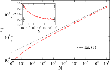
Figure 2: The average number of frozen aggregates $F$ versus system size $N$. The inset shows the growth exponent $\alpha(N)\equiv d\ln F/d\ln N$ versus $N$. The limiting value $\alpha\equiv\lim_{N\to\infty}\alpha(N)$ quoted in Eq. (1) was obtained by noting that $\alpha(N)$ is linear $1/F$ when $N$ is sufficiently large.

The aggregation processes (2a)–(2b) are symmetric with respect to orientation, and as long as the initial conditions are also symmetric, we expect that statistical properties of the horizontal size and of the vertical size are equivalent. Yet, as we discuss below, the width $\omega$ and the length $\ell$ defined as

$$\omega={\rm min}(i,j),\qquad\ell={\rm max}(i,j),$$ (3)

are not statistically equivalent.

For sufficiently-large systems, we find that the jammed state contains two rectangles of width $\omega=1$: one of horizontal size $i=1$, and one of vertical size $j=1$. Similarly, there are two rectangles of width $\omega=2$, two rectangles of width $\omega=3$, and so on. For instance, we quote the ordered widths of the $f=13$ frozen rectangles

$$\{1,1,2,2,3,3,4,4,5,5,6,7,9\}\,,$$ (4)

that emerged in a simulation of a system of size $N=10^{4}$ where $F=13.2$ and $\sigma=1.2$. We note that there may be one or two rectangles of a given width, and that the width sequence may contain gaps. We characterize this sequence using the maximal width $\omega_{\rm max}$ and the maximal width for which there is a pair of rectangles, $\omega_{\rm pair}$; for the sequence (4), $\omega_{\rm max}=9$ and $\omega_{\rm pair}=5$. Our simulations confirm that both averages $\langle\omega_{\rm max}\rangle$ and $\langle\omega_{\rm pair}\rangle$ follow the growth law (1). We deduce that the typical width grows as the total number of frozen aggregates,

$$w\sim N^{\alpha}\,.$$ (5)

$\omega$	$1$	$2$	$3$	$4$	$5$	$6$
$m_{\omega}$	$0.622$	$0.182$	$0.0694$	$0.0365$	$0.0214$	$0.0139$
$M_{\omega}$	$0.622$	$0.804$	$0.873$	$0.910$	$0.931$	$0.945$

Table 1: The area fraction $m_{\omega}$ and the cumulative area fraction $M_{\omega}=\sum_{\nu\leq\omega}m_{\nu}$ versus the width $\omega$.

A striking feature of the jammed state is that frozen rectangles of finite width contain a finite fraction of the total area. In particular, the two rectangles with width $\omega=1$ contain a fraction $m_{1}=0.622$ of all area, while the two rectangles with width $\omega=2$ contain a fraction $m_{2}=0.182$ of all area. Generally, the fraction $m_{\omega}$ of all area in rectangles of width $\omega$ approaches a constant in the limit $N\to\infty$. Table 1 lists $m_{\omega}$ and its cumulative sum for $1\leq\omega\leq 6$. Remarkably, rectangles with width $\omega\leq 6$ contain nearly $95\%$ of the total area. The area fraction is normalized,

$$\sum_{\omega=1}^{\infty}m_{\omega}=1\,.$$ (6)

We stress that $m_{\omega}$ may fluctuate when $N$ is finite, but it becomes deterministic in the limit $N\to\infty$. Moreover, the area $A_{\omega}$ of rectangles with width $\omega$ is a random quantity with average $\langle A_{\omega}\rangle\simeq m_{\omega}N$ and variance $\langle A_{\omega}^{2}\rangle-\langle A_{\omega}\rangle^{2}\sim N$.

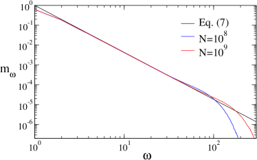
Figure 3: The area fraction $m_{\omega}$ versus width $\omega$, obtained from simulations with $N=10^{8}$ and $N=10^{9}$. Also shown For reference is the theoretical prediction (7) with the exponent $\alpha$ from Eq. (1).

The length of rectangles of width $\omega$ is proportional to system size, $\simeq m_{\omega}N/(2\omega)$, so their aspect ratio scales as $m_{\omega}N/(2\omega^{2})$. The quantity $m_{\omega}$ decreases with width and by definition, the aspect ratio must be larger than unity. We now postulate that the aspect ratio of the widest rectangles is of order unity and hence, $m_{\omega}\sim w^{2}/N$. By using the scaling behavior $N\sim w^{1/\alpha}$ which follows from (5), we arrive at our second major result that the area fraction decays algebraically with width (figure 3)

$$m_{\omega}\sim\omega^{-\gamma},\qquad\gamma=\alpha^{-1}-2\,$$ (7)

when $\omega\gg 1$. Our numerical simulations support this theoretical prediction. We also note that the normalization (6) sets the bounds $\gamma>1$ and $\alpha<1/3$.

In a finite system, the power-law decay (7) holds up to the scale $w\sim N^{\alpha}$ which also characterizes the widest rectangles. Interestingly, rectangles of finite width $\omega={\cal O}(1)$ have an area proportional to system size, $A\sim N$, but otherwise, rectangles with the typical width $w\sim N^{\alpha}$ have an area that grows sublinearly with system size $A\sim w^{2}\sim N^{2\alpha}$. The former rectangles have a large aspect ratio that is proportional to system size, while the latter have an aspect ratio of order one. Consequently, a finite number of clusters have a macroscopic area, while typical clusters contains a vanishing fraction $N^{2\alpha-1}$ of total area.

III Aggregation Kinetics

We now turn our attention to the time-dependent evolution toward the jammed state. Let $R_{i,j}(t)$ be the density of rectangles with horizontal size $i$ and vertical size $j$ at time $t$. This quantity satisfies the rate equation

$$\frac{dR_{i,j}}{dt} = \sum_{i_{1}+i_{2}=i}R_{i_{1},j}R_{i_{2},j}-2R_{i,j}\sum_{k\geq 1}R_{k,j}$$

$$+ \sum_{j_{1}+j_{2}=j}R_{i,j_{1}}R_{i,j_{2}}-2R_{i,j}\sum_{k\geq 1}R_{i,k},$$

and is subject the initial condition $R_{i,j}(0)=\delta_{i,1}\delta_{j,1}$. The evolution equation (III) is a straightforward generalization of the Smoluchowski equations for coagulation mvs16 ; mvs17 ; fl ; krb . The first two terms on the right-hand side account for the aggregation process (2a), with the first term describing gain of a single large rectangle and the second term describing loss of two small rectangles. Similarly, the last two terms account for the complementary process (2b). The rate equations are mean-field in nature and reflect that all pairs of rectangles interact at the same rate, set to unity without loss of generality. In writing (III), we assumed that the system is infinite. The aggregation process conserves area, and accordingly the rate equations (III) conserve the area density $\sum_{i,j}(ij)R_{i,j}$. Finally, we expect the size density to be symmetric, $R_{i,j}=R_{j,i}$, because the rate equations and the initial conditions are symmetric.

The overall density of rectangles $\rho=\sum_{i,j}R_{i,j}$ decays with time according to the rate equation

$$\frac{d\rho}{dt}=-\left(\sum_{i,j,k}R_{i,j}R_{k,j}+\sum_{i,j,k}R_{i,j}R_{i,k}\right)\,.$$ (9)

This equation is obtained by summing (III) over both indices, and it reflects that in each aggregation event, the total number of aggregates decreases by one. The two loss terms account for the two aggregation processes in (2a)–(2b). Unlike ordinary aggregation, the density does not obey a closed equation; more generally, moments of the size distribution do not obey closed equations.

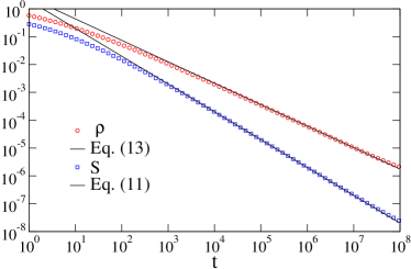
Figure 4: The density of aggregates $\rho$ and the density of sticks $S$ versus time $t$, obtained from numerical simulations with $N=10^{8}$. Also shown for reference are the theoretical predictions (11) and (13).

The rate equations (III) appear to be analytically intractable. Nevertheless, we can gain insights from these equations by considering the density of “sticks”, $S=\sum_{j}R_{1,j}$, namely, rectangles with minimal horizontal size, $i=1$. By symmetry, $S$ is also the density of rectangles with minimal vertical size, $S=\sum_{i}R_{i,1}$. By summing (III) over $j$, we find

$$\frac{dS}{dt}=-S^{2}-2\sum_{i,j}R_{1,j}R_{i,j},$$ (10)

with $S(0)=1$. The first loss term corresponds to a merger of two sticks along the vertical side, while the second term corresponds to a merger of a stick with a rectangle along the horizontal side.

Based on properties of the jammed state, we argue that the first term in (10) is dominant in the long-time limit. Each aggregation event reduces the total number of aggregates by one. When a finite system of size $N$ ends up with $f$ frozen aggregates, the total number of aggregation events equals $N-f$. Moreover, each aggregation event generating a stick necessarily involves two sticks. Since frozen sticks have the macroscopic area $\simeq m_{1}N$ with $m_{1}>1/2$, we arrive at the remarkable conclusion that in the majority of all aggregation events, two sticks combine into a larger stick. Consequently, the first term in (10) is dominant, leading to the closed rate equation $dS/dt=-S^{2}$ and the power-law decay (Fig. 4)

$$S\simeq t^{-1}\,.$$ (11)

The simulations confirm that the decay exponent and the prefactor both equal unity: hence, this behavior is asymptotically exact.

In a finite system, the expected number of sticks with minimal horizontal size decays as the product of system size and density (11), that is, $\simeq Nt^{-1}$. As discussed in section II, the jammed state contains two sticks. Therefore, the jamming time $\tau$ is simply proportional to system size,

$$\tau\sim N\,.$$ (12)

Furthermore, the total density $\rho$ is bounded from below by the stick density, $\rho\geq S$. In view of the time-dependent behavior (11), we expect that the density decays algebraically with time, $\rho\sim t^{-\beta}$. In a finite system, the average number of rectangles scales as $N\rho(t)\sim Nt^{-\beta}$. By substituting the linear jamming time (12) into $N\rho(\tau)$ and matching to the average number of frozen rectangles in (1), we conclude that $\alpha+\beta=1$. Therefore, the exponent $\alpha$ also governs the decay of the density (Fig. 4)

$$\rho\sim t^{\alpha-1}\,.$$ (13)

The size distribution of sticks yields additional insights about the aggregation kinetics. Both the first loss term in (10) and the consequent asymptotic behavior (11) are precisely the same as in ordinary aggregation where each aggregate is characterized solely by its mass krb . The size distribution $R_{1,\ell}$ of sticks with minimal horizontal size and vertical size $\ell$ obeys

$$\frac{dR_{1,\ell}}{dt}\!=\!\sum_{i+j=\ell}R_{1,i}R_{1,j}\!-\!2SR_{1,\ell}\!-\!2\left(\sum_{i}R_{i,\ell}\right)R_{1,\ell}\,,$$ (14)

with the initial condition $R_{1,\ell}(0)=\delta_{1,\ell}$. The first two terms describe aggregation events of the type (2a) that involve two sticks. Because the asymptotic behavior (11) is exact, we expect that theses two terms are dominant, while the last term, which corresponds to aggregation events of the type (2b), is asymptotically negligible.

By dropping the last term in Eq. (14), we recover the standard Smoluchowski rate equation for the size distribution in ordinary coalescence. In the long-time limit, the size distribution is purely exponential (Figure 5)

$$S_{1,\ell}\simeq\frac{2}{m_{1}t^{2}}\,e^{-2\ell/(m_{1}\,t)}\,.$$ (15)

This scaling behavior is consistent with the decay (11), and the limiting size of frozen sticks $\sum_{\ell}\ell S_{1,\ell}\to m_{1}/2$ as $t\to\infty$. According to Eq. (15), stick length grows linearly with time, $\ell\sim t$.

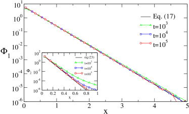
Figure 5: The scaling functions $\Phi_{1}(x)$ and $\Phi_{2}(x)$ versus the scaling variable $x=l/t$.

Our numerical simulations suggest that rectangles with finite width are statistically similar to sticks. Let $\mathcal{R}_{\omega,l}(t)$ be the density of rectangles with width $\omega$ and length $\ell$, using the definitions (3). This size distribution adheres to the scaling form (Figure 5)

$$\mathcal{R}_{\omega,\ell}(t)\simeq t^{-2}\,\Phi_{\omega}\big{(}\ell\,t^{-1}\big{)}\,,$$ (16)

as in Eq. (14). The scaling function $\Phi_{\omega}$ quantifies the density of sticks with length $\ell$ and width $\omega$. This function is always exponential, although the decay constant and the normalization depend on width (Figure 5)

$$\Phi_{\omega}(x)=2\mu_{\omega}\,e^{-\mu_{\omega}x}\,,\quad\mu_{\omega}=2\omega/m_{\omega}\,.$$ (17)

According to equations (16)–(17), rectangles with width $\omega$ contain a fraction $m_{\omega}$ of the total area, $\sum_{\ell}\omega\ell\mathcal{R}_{\omega,\ell}\to m_{\omega}$ as $t\to\infty$. Moreover, the density $U_{\omega}=\sum_{\ell}\mathcal{R}_{\omega,\ell}$ of rectangles with width $\omega$ and length $\ell$ decays algebraically with time,

$$U_{\omega}\simeq 2\,t^{-1}\,.$$ (18)

This behavior can be obtained by repeating the steps leading to (11), which describes the stick density, $S\simeq U_{1}/2$. The scaling behavior (16)–(17) also shows that the average length of rectangles with width $\omega$ grows linearly with time, $\langle\ell_{\omega}\rangle\sim(m_{\omega}t)/(2\omega)$, or equivalently, $\langle\ell_{\omega}\rangle\simeq v_{\omega}t$, with the growth velocity $v_{\omega}=m_{\omega}/(2\omega)$.

Figure 6: Illustration an aggregation process of the type (2a) which increases the width.

Generally, merger events can lead to either wider or longer rectangles. Figures 1 and 6 both depict merger events of the type (2a). In the first scenario, the width stays the same, but the length grows. However, in the second scenario, the length stays the same, but width grows. Thus far, we have seen that: (i) in a finite system, frozen rectangles with finite width are macroscopic, (ii) the typical length of rectangles with finite with grows linearly width time, and (iii) the scaling function underlying the size distribution is exponential as in ordinary aggregation. All these results suggest that elongation events are dominant.

The scaling behavior (16)–(17) applies for finite $\omega$ in the long-time limit. Yet, the typical width does grow, albeit slowly, with time

$$\omega\sim t^{\alpha}.$$ (19)

This scale is consistent with the growth law (1) and the jamming time (12), and it can also be obtained by substituting the density (13) and the width (18) into the estimate $\rho\sim w\,U_{w}$. As shown in Figure 7, the scaled width distribution becomes a universal function of the scaled width

$$U_{\omega}(t)\simeq t^{-1}\phi(\omega t^{-\alpha})\,.$$ (20)

Equation (18) sets the scaling of the distribution, while the growth law (19) sets the scaling of the width. The small-$z$ behavior is simply $\phi(0)=2$. Moreover, simulations suggest that relatively wide rectangles are very rare as the large-$z$ tail is roughly Gaussian, $\phi(z)\sim\exp(-{\rm const.}\times z^{2})$ for $z\gg 1$.

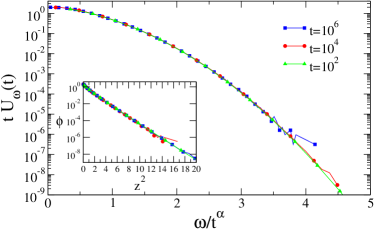
Figure 7: The scaled width distribution $t\,U_{\omega}(t)$ versus the scaled width $\omega/t^{\alpha}$. The inset shows the large $z$ tail of the scaling function $\phi(z)$.

Next, we study the density $P(a,t)$ of rectangles with area $a$ at time $t$. This quantity satisfies the sum rules

$$\sum_{a}P(a,t)=\rho,\qquad\sum_{a}aP(a,t)=1\,.$$ (21)

In section II, we noted that while rectangles with finite width have diverging aspect ratio, rectangles with the typical width (5) have finite aspect ratio. Thus, we expect that the typical width (19) governs the typical area, $a\sim w^{2}\sim t^{2\alpha}$. Consequently, the area distribution adheres to the scaling form (Figure 8)

$$P(a,t)\sim t^{-1-\alpha}\,\varphi\left(a\,t^{-2\alpha}\right)\,.$$ (22)

Here, the time-dependent prefactor ensures that the total density, given by the first sum in (21), decays as in (13).

The scaling function underlying the area distribution, $\varphi(z)$, has two algebraic tails

$$\varphi(y)\sim\begin{cases}y^{(3-\alpha)/(2\alpha)}&y\ll 1,\\ y^{-(1-\alpha)/(1-2\alpha)}&y\gg 1.\end{cases}$$ (23)

The maximal area grows linearly with time, $a_{\rm max}\sim t$, and the summation in (21) should therefore be carried up to that scale, $\sum_{a=1}^{t}a\,P(a,t)\sim 1$. The algebraic large-$y$ tail is set by this sum which reflects area conservation. The minimal area, $a_{\rm min}=1$, corresponds to tiles. The density of tiles, $T\equiv R_{1,1}$, decays quite rapidly, $T\sim t^{-4}$, as follows from $dT/dt=-4ST$ and the stick density (11). This rapid decay sets the remarkably sharp small-$y$ tail in (23). The two algebraic tails in (23) indicate that the area distribution is very broad and that the system may contain rectangles with areas much smaller than or much larger than the typical area, $1\ll a\ll t$. In contrast, the length distribution and the width distribution are much narrower, with exponential and Gaussian tails, respectively.

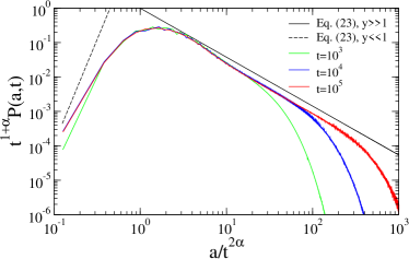
Figure 8: The scaled area distribution $t^{1+\alpha}P(a,t)$ versus the scaled area $a/t^{2\alpha}$.

The scaling behaviors above show that the exponent $\alpha$ governs key features of the kinetics including the decay of the density (13), the typical width (19), the width distribution (20), and the area distribution (22). Based on these scaling behaviors we postulate that the joint size distribution exhibits the scaling behavior

$$R_{i,j}(t)\sim t^{-1-\alpha}G(it^{-\alpha},jt^{-\alpha})\,.$$ (24)

To comply with the decay law (13), the integral of the scaling function $\iint d\xi d\eta\,G(\xi,\eta)$ must be finite. Also, area conservation sets $\iint d\xi d\eta\,\xi\eta\,G(\xi,\eta)\sim t^{1+\alpha}$ where the upper limit of integration for both $\xi$ and $\eta$ is of the order $t^{1-\alpha}$. We did not verify the form (24), but nevertheless, we did confirm one of its implications. The density of squares, $H(t)=\sum_{i}R_{i,i}(t)$, is indeed proportional to the inverse of time, $H\sim t^{-1}$, as follows from (24). Moreover, the average number of squares in the frozen state is of order unity as $NH(\tau)\sim 1$. This prediction is consistent with properties of the jammed state where the widest rectangle has aspect ratio of order unity, while its area is typically the smallest.

We now examine the evolution of the area fraction $m_{\omega}(t)$, defined as the fraction of the total area contained in rectangles with width $\omega$ at time $t$. This quantity changes only when two rectangles with the same length merge into a wider rectangle as illustrated in Figure 6. The fractions $m_{\omega}$ evolve according to

$$\frac{dm_{\omega}}{dt}\!=\!2\!\sum_{i+j=\omega}\!\sum_{\ell}\omega\ell\mathcal{R}_{i,\ell}\mathcal{R}_{j,\ell}\!-\!4\sum_{j}\sum_{\ell}\omega\ell\mathcal{R}_{j,\ell}\mathcal{R}_{\omega,\ell}\,.$$ (25)

The first term accounts for gain of area by rectangles of width $\omega$, and the last term, for loss of area from such rectangles. One can check that the rate equation (25) conserves the total area $(d/dt)\sum_{\omega}m_{\omega}=0$.

For finite width $\omega$, and in the limit $t\to\infty$, we substitute the exponential length distribution (16)-(17) into the rate equation (25). We then convert sums over $\ell$ into integrals, $\sum_{\ell\geq 1}\to\int_{1}^{\infty}d\ell$. The resulting rate equation for the area fraction $m_{\omega}$ satisfies $dm_{\omega}/dt\simeq-C_{\omega}\,t^{-2}$ with the constants

$$C_{\omega}=-2\omega\sum_{i+j=\omega}\frac{\mu_{i}\mu_{j}}{(\mu_{i}+\mu_{j})^{2}}+4\omega\sum_{j}\frac{\mu_{\omega}\mu_{j}}{(\mu_{\omega}+\mu_{j})^{2}}\,,$$ (26)

and $\mu_{\omega}=2\omega/m_{\omega}(\infty)$. Therefore, the relaxation of the area fraction toward the limiting value is similar to (18),

$$m_{\omega}(t)-m_{\omega}(\infty)\simeq C_{\omega}\,t^{-1}\,,$$ (27)

as $t\to\infty$. Using the fractions $m_{\omega}$ that were obtained from numerical simulations (see Table 1 and figure (3)), we have $C_{1}=1.7$ and $C_{2}=4.8$. Numerically, we verified that $m_{1}(t)$ and $m_{2}(t)$ evolve according to (27).

Equation (27) shows that the area fraction decreases monotonically when $t\to\infty$. Moreover, the growth law (19) suggests that there is a time scale $t_{\omega}\sim w^{1/\alpha}$ which characterizes the buildup and discharge of area at width $\omega$. At early times, $t\ll\omega^{1/\alpha}$, the area fraction $m_{\omega}$ increases with time, and at late times, $t\gg\omega^{1/\alpha}$, the area fraction decreases with time. We thus anticipate $m_{\omega}(t_{\omega})\propto m_{\omega}(\infty)$, and using the tail of the area fraction (7), we find that the constants in (26) are quadratic

$$C_{\omega}\sim\omega^{2}\,.$$ (28)

Our results show that rectangles grow by two separate processes which govern the length and the width. In the majority of aggregation events, the width stays the same but the length grows. This aggregation process reduces to ordinary one-dimensional aggregation, allowing us to obtain exact statistical properties of the length which grows linearly with time. A minority of aggregation events increase the width while keeping the length unchanged. This is a much slower process as the width grows sub-linearly with time, with a rather small growth exponent. Obtaining exact statistical properties of the width and in particular, obtaining the growth exponent $\alpha$ requires a solution of the full rate equations (III) with the two-variable scaling form (24)

IV Planar Aggregation

We now discuss a complementary aggregation process involving rectangles that are embedded in two-dimensional space. Initially, the system consists of $N$ identical tiles with $i=j=1$. These tiles form a two-dimensional grid with linear dimension $L$, and hence, area $N=L^{2}$. In each successful aggregation event, two neighboring rectangles merge and form a larger rectangle.

Figure 9: A jammed configuration in a system of size $N=10^{4}$.

There are several ways to realize this planar process. In our implementation, in each aggregation attempt, one rectangle is chosen at random, and additionally, one of its four sides is chosen at random. If this side is shared with a neighboring rectangle, the two rectangles merge into a larger rectangle as in (2a) and(2b). Time is augmented by the inverse of the number of rectangles after each aggregation attempt.

In planar aggregation, each rectangle interacts only with nearest neighbors, in contrast with the mean-field version where each rectangle interacts with all other rectangles. Nevertheless, both systems arrive at a jammed state where aggregation is no longer possible. In a jammed configuration, two neighboring rectangles never share a side. Figure 9 shows a jammed state in a system of size $N=10^{4}$.

The jammed state is fascinating as it represents a planar tiling where the original two-dimensional grid is covered by rectangles. Our process differs from dimer tiling pwk ; ft ; mef ; ehl ; rjb ; cep ; ckp in that rectangles are heterogeneous and in that there is a constraint that two neighboring rectangles in the jammed state never share a side. Tiling is relevant to thin films growth sm and DNA self-assembly llry . We also note that fragmentation of two-dimensional space, which is the opposite process to the aggregation considered in this study, also generates tiling by rectangles kb94 .

$\rho_{\infty}$	$T_{\infty}$	$S_{\infty}$	$H_{\infty}$
$0.1803$	$9.949\times 10^{-3}$	$0.1322$	$2.306\times 10^{-2}$

Table 2: The jamming densities of rectangles, tiles, sticks, and squares. These densities were obtained by plotting for example $\rho(L)$ versus $L^{-1}$ and using a linear fit.

Qualitatively, the jammed state exhibits orientational ordering as the orientation of neighboring rectangles are correlated. This correlation is short-ranged. Further, rectangles tend to be larger along the boundary, and they also tend to be aligned with the boundary. For example, the north and south boundaries have an overpopulation of horizontal rectangles.

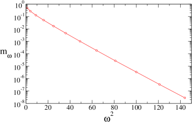
Figure 10: The area fraction $m_{\omega}$ for planar rectangular aggregation, from simulations with system size $N=10^{8}$.

The rectangular tiling can be characterized in several ways. For example, the average aspect ratio equals $3.39$. Further, we measured the jamming densities of rectangles $\rho_{\infty}$, tiles $T_{\infty}$, sticks $S_{\infty}$, and squares $H_{\infty}$ (see Table II). In measuring these densities, we noticed that finite-size corrections are inversely proportional to the linear dimension $L$, $\rho(L)-\rho_{\infty}\sim L^{-1}$. This behavior suggests that boundary effects extend only a finite distance from the boundary, and also, that the correlation length characterizing the orientational order is finite. The finite density of jammed rectangles, $\rho_{\infty}=0.1803$, indicates that the average number of frozen rectangles grows linearly with system size,

$$F\sim N\,.$$ (29)

This contrasts with the mean-field case where the growth is sub-linear.

We also note that the vast majority of intersections involve three rectangles, although intersections may rarely be formed by four rectangles. In the initial state, the tiles form a perfect grid with each lattice vertex surrounded by four tiles. We measured $v_{n}$, the density of vertices that are surrounded by $n$ rectangles in the jammed state, with $\sum_{n=1}^{4}v_{n}=1$. Internal vertices are surrounded by a single rectangle, while vertices surrounded by $n=3$ or $n=4$ rectangles correspond to intersections. The vertex densities, listed in table III, show that a fraction $v_{3}/(v_{3}+v_{4})=0.988$ of all intersections are formed by three rectangles, while the complementary fraction $v_{4}/(v_{3}+v_{4})=0.012$ of all intersections are formed by four rectangles.

$n$	$1$	$2$	$3$	$4$
$v_{n}$	$0.215$	$0.429$	$0.352$	$4.26\times 10^{-3}$

Table 3: The vertex densities $v_{n}$.

We also measured the quantity $m_{\omega}$, the fraction of the total area in rectangles of width $\omega$. Figure 10 shows that the area fraction has a sharp, Gaussian, tail

$$m_{\omega}\sim\exp\left(-{\rm const.}\times\,\omega^{2}\right),$$ (30)

for $\omega\gg 1$. This decay is much sharper compared with the power-law behavior (7) in the mean-field case. Consequently, for $\omega\leq 5$, the quantity $m_{\omega}$ is larger in the planar case (Table IV).

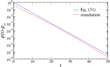
Figure 11: The time-dependent density $\rho(t)-\rho_{\infty}$ versus time.

To characterize the approach toward the jammed configuration, we measured the time-dependent density, and find that the relaxation is exponential (figure 11)

$$\rho(t)-\rho_{\infty}\sim e^{-c\,t}\,.$$ (31)

with $c=0.34$. This approach is much faster than the algebraic decay (13) that occurs when all pairs of rectangles may interact.

$\omega$	$1$	$2$	$3$	$4$	$5$	$6$
$m_{\omega}$	$0.525$	$0.273$	$0.128$	$0.0516$	$0.0170$	$0.00458$

Table 4: The fraction of the total area $m_{\omega}$ contained in frozen rectangles of width $\omega$.

Aggregation of rectangles embedded in a plane has very different features compared with the mean-field case. The relaxation toward the jammed state is very fast, jammed rectangles have size and area of the order unity, and the number of frozen rectangles is proportional to system size.

V Conclusions

We studied an aggregation process where rectangles with compatible sides combine to form larger rectangles. This process results in a jammed state where each rectangle has two unique dimensions. Aggregation of rectangles exhibits many interesting features. Some properties of the final state are deterministic while others are random. For example, the fraction of area in rectangle of finite width becomes a deterministic quantity in the long-time limit. However, the number of rectangles in the jammed state is random and it fluctuates from one realization to another.

While the aggregation process is symmetric with respect to the horizontal and the vertical sides, there are two different mechanism that control the growth of the width and the length. In the majority of aggregation events, two rectangles with the same width combine and form a longer rectangle with a larger aspect ratio. There are also rare events where two aggregates of the same length combine to form a wider rectangle with smaller aspect ratio. Moreover, two distinct scaling laws characterize the growth of the width and the length.

The growth exponent $\alpha$, which characterizes the growth of the number of frozen aggregates with system size also governs scaling properties of the time-dependent behavior. In particular, the width distribution and the area distribution both adhere to scaling forms in the long-time limit, and the exponent $\alpha$ characterizes both of these scaling behaviors. Using heuristic scaling arguments, we related all power-law exponents that arise in the system to the growth exponent $\alpha$. Aggregation of rectangles is a special case of multi-component aggregation as each cluster is characterized by two sizes. Two distinct growth exponents can emerge in multi-component aggregation processes, yet, when there are as many conservation laws as there are components, the scaling exponents can be obtained using dimensional analysis kb96 ; vz ; lbd ; fg ; mm . The aggregation process in this study has a single conservation law, and as a result, the growth exponent $\alpha$ does not follow from heuristic scaling arguments.

We presented results for a specific realization of the aggregation process for which the rate equation (III) is exact. Yet, we verified that other variants of this process exhibit a similar behavior. First, we checked that the growth exponent $\alpha$ in Eq. (1) is robust even when the vertical channel (2a) and the horizontal channel (2b) are realized with different rates. Second, we considered the situation where aggregates can rotate in order to maximize the fraction of successful aggregation attempts. Again, we found that the scaling properties are robust, although quantities such as the area fraction are sensitive to the details of the merger process.

We also explored aggregation of $d$-dimensional hyper-rectangles or “boxes.” In general, we require that two boxes have a matching ($d-1$ dimensional) facet, such that two boxes combine along this matching facet to form a larger box. Generally, the system reaches a jammed state where the expected number of rectangles grows algebraically with system size as in (1). The growth exponent $\alpha$ increases with the spatial dimension: $\alpha=0$, $0.23$, $0.33$, and $0.40$, for $d=1$, $2$, $3$, and $4$. The aggregation process becomes less effective as the dimension increases and $\alpha\to 1$ when $d\to\infty$.

We also studied a planar realization where only neighboring rectangles may interact. In this case, the system reaches a jammed state that is a special rectangular tiling of the plane where two neighboring rectangles never share a matching side. Statistical properties of the jammed state are quite different compared with the case where all rectangles interact. In particular, the number of frozen rectangles is proportional to system size, and the relaxation toward this state is exponentially fast. An interesting open question is the entropy of the jammed configuration. We expect the number of jammed configurations to grow exponentially with system size, and it would also be interesting to find out if the entropy of the jammed state depends on the shape of domain, as is the case for dimer tiling jb ; nd .

References

- (1) M. V. Smoluchowski, Phys. Zeit. 17, 557 (1916).
- (2) M. V. Smoluchowski, Z. Phys. Chem. 92, 129 (1917); ibid 92, 155 (1917).
- (3) F. Leyvraz, Phys. Rep. 383, 95 (2003).
- (4) P. L. Krapivsky, S. Redner and E. Ben-Naim, A Kinetic View of Statistical Physics (Cambridge University Press, Cambridge, 2010).
- (5) P. J. Flory, J. Amer. Chem. Soc. 63, 3083 (1941).
- (6) W. H. Stockmayer, J. Chem. Phys. 11, 45 (1943).
- (7) P. J. Flory, Principles of Polymer Chemistry (Cornell University Press, Ithaca, 1953).
- (8) S. Chandrasekhar, Rev. Mod. Phys. 15, 1 (1943).
- (9) C. Dominik and A. G. G. M Tielens, Astrophys. Jour. 480, 647 (1997).
- (10) N. Brilliantov, P. L. Krapivsky, A. Bodrova, F. Spahn, H. Hayakawa, V. Stadnichuk, and J. Schmidt, Proc. Natl. Acad. Sci. USA 112, 9536 (2015).
- (11) S. K. Frielander, Smoke, Dust and Haze: Fundamentals of Aerosol Behavior (Wiley, New York, 1977).
- (12) G. Falkovich, A. Fouxon, and M. G. Stepanov, Nature 419, 151 (2002).
- (13) W. W. Grabowski and L. P. Wang, Ann. Rev. Fluid. Mech. 45, 293 (2013).
- (14) A. Pumir and M. Wilkinson, Ann. Rev. Cond. Matt. Phys. 7, 141 (2016).
- (15) B. Bollobás, Random Graphs (Academic Press, London, 1985).
- (16) S. Janson, T. Łuczak, and A. Rucinski, Random Graphs (John Wiley & Sons, New York, 2000).
- (17) S. N. Dorogovtsev and J. F. F. Mendes, Evolution of Networks: From Biological Nets to the Internet and WWW (Oxford University Press, Oxford, UK, 2003).
- (18) M. E. J. Newman, Networks: An Introduction (Oxford University Press, Oxford, 2010).
- (19) P. L. Krapivsky and S. Redner, Phys. Rev. E 54, 3553 (1996).
- (20) S. N. Majumdar, S. Krishnamurthy, and M. Barma, Phys. Rev. Lett. 81, 3691 (1998).
- (21) R. Rajesh and S. N. Majumdar, Phys. Rev. E 63, 036114 (2001).
- (22) R. M. Ziff, E. M. Hendriks, and M. H. Ernst, Phys. Rev. Lett. 49, 593 (1982).
- (23) R. Botet and R. Jullien, J. Phys. A 17, 2517 (1984).
- (24) A. A. Lushnikov, Phys. Rev. Lett. 93, 198302 (2004).
- (25) E. Ben-Naim and P.L. Krapivsky, J. Phys. A 38, L417 (2005).
- (26) E. R. Domilovskii, A. A. Lushnikov, and V. N. Piskunov, Dokl. Phys. Chem. 240, 108 (1978).
- (27) E. M. Hendriks, M. H. Ernst, and R. M. Ziff, J. Stat. Phys. 31, 519 (1983).
- (28) J. L. Spouge, J. Colloid Inter. Sci. 107, 38 (1985).
- (29) P. G. J. van Dongen, J. Phys. A 20, 1889 (1987).
- (30) N. V. Brilliantov and P. L. Krapivsky, J. Phys. A 24, 4787 (1991).
- (31) Ph. Laurençot, Nonlinearity 12, 229 (1999).
- (32) L. Malyushkin and J. Goodman, Icarus 150, 314 (2001).
- (33) E. Ben-Naim and P.L. Krapivsky, Phys. Rev. E 68, 031104 (2003)
- (34) E. Ben-Naim and P.L. Krapivsky, Phys. Rev. E 77, 061132 (2008).
- (35) P. W. Kasteleyn, Physica 27, 1209 (1961).
- (36) M. E. Fisher and H. Temperley, Phil. Mag. 6, 1061 (1961).
- (37) M. E. Fisher and J. Stephenson, Phys. Rev. 132, 1411 (1963).
- (38) E. H. Lieb, J. Math. Phys. 8, 2339 (1967).
- (39) R. J. Baxter, J. Math. Phys. 9, 650 (1968).
- (40) H. Cohn, N. Elkies, and K. Propp, Duke Math. J. 85, 117 (1996).
- (41) H. Cohn, R. Kenyon, and K. Propp, J. Amer. Math. Soc. 14, 297 (2001).
- (42) R.E. Schaak and T.E. Mallouk, Chem. of Mater. bf 12, 2513 (2000).
- (43) C. X. Lin, Y. Liu, S. Rinkler, and H. Yan, Chem. Phys. Phys. Chem. 7, 1641 (2006).
- (44) P. L. Krapivsky and E. Ben-Naim, Phys. Rev. E 50, 3502 (1994).
- (45) P.L. Krapivsky and E. Ben-Naim, Phys. Rev. E 53, 291 (1996).
- (46) R.D. Vigil and R.M. Ziff, Chem. Eng. Sci 53, 1725 (1998)
- (47) I.J. Laurenzi, J. D. Bartels, and S.L. Diamond, J. Comp. Phys. 177, 418 (2002).
- (48) J.M. Fernandez-Diaz and G.J. Gomez-Garcia, EPL 78, 56002 (2007).
- (49) T. Matsoukas and C.L. Marshall, EPL 92, 46007 (2010).
- (50) D. Joseph and M. Baake, J. Phys. A 29, 6709 (1996).
- (51) N. Destainville, J. Phys. A 31 6123 (1998).