Hybrid multilane models for highway traffic

Abstract

We study effects of lane changing rules on multilane highway traffic using the Nagel-Schreckenberg cellular automaton model with different schemes for combining driving lanes (lanes used by default) and overtaking lanes. Three schemes are considered: a symmetric model, in which all lanes are driving lanes; an asymmetric model, in which the right lane is a driving lane and the other lanes are overtaking lanes; a hybrid model, in which the leftmost lane is an overtaking lane and all the other lanes are driving lanes. In a driving lane vehicles follow symmetric rules for lane changes to the left and to the right, while in an overtaking lane vehicles follow asymmetric lane changing rules. We test these schemes for three- and four-lane traffic mixed with some low-speed vehicles (having a lower maximum speed) in a closed system with periodic boundary conditions as well as in an open system with one open lane. Our results show that the asymmetric model, which reflects the ”Keep Right Unless Overtaking” rule, is more efficient than the other two models. An extensible software package developed for this study is free available.

I Introduction

Transport phenomena arise in a wide variety of many-particle systems, ranging from vehicular traffic to physical or biological systems, such as fluid flow, molecular motor transport and more. Among all theoretical transport models, the totally asymmetric simple exclusion process (TASEP) is the most widely applied paradigm for transport of interacting particles 1dTASEP . The TASEP consists of particles moving unidirectionally on a one-dimensional lattice with the constraint that at any given time every lattice site can be occupied at most by one particle. The Nagel-Schreckenberg (NaSch) cellular automaton model NaSch , a standard model for the simulation of highway traffic, can be regarded as an extension of the TASEP in which the maximum speed of particles (vehicles), acceleration and random deceleration are introduced to mimic some basic phenomena in highway traffic, such as spontaneous formation of congestion. The flexibility of the NaSch cellular automaton approach allows one to generate various versions of the model to study different aspects of traffic problems. While many results are known for the single-lane model 1dTASEP ; Rev , there remains much scope for further study on multilane generalizations. For example, in multilane traffic models different types of the lane-changing rules can lead to considerably different results; therefore, one expects that lane-changing rules in real traffic can have significant impact on traffic flows.

A large number of lane-changing rules have been considered in many previous studies to reproduce various empirically observed phenomena (see Rev ; Nagel_PRE ; Knospe ; Lee ; Habel ; Su ). Instead of proposing new decision-making rules and criteria for lane changes, here we focus on effects of different arrangements of lanes on multilane highway traffic. We present an extensible C++ package (available in CODES ) for implementing the multilane NaSch model with a set of tunable parameters and conditions, including the number of lanes (any positive integer), lane-changing rules, boundary conditions of each lane, and more. The significance of this package is its user-definable settings for the individual lanes. Using this software package we consider three types of lane arrangements implemented on the NaSch model with more than two lanes, corresponding to three different lane-changing models: (1) the symmetric model, in which overtaking is allowed on the left and also on the right in all lanes; (2) the asymmetric model, in which the right lane is used by default and overtaking has to be on the left; (3) the hybrid model, in which the leftmost lane is the overtaking lane while the other lanes are treated as in the symmetric model. The hybrid model describes multilane highway traffic observed in many countries where only the lane closest to the median strip is designed for overtaking and overtaking on the right is not considered to be a driving offense. By comparing the traffic flow at a fixed number density of vehicles in closed systems and the average velocity in open systems, we demonstrate that for heterogeneous traffic consisting of different types of vehicles (fast and slow vehicles) the asymmetric model is more efficient than the other two models. Here and throughout the paper we consider ”right-hand traffic”, for ”left-hand traffic” implemented such as in the UK and Japan ”left” and ”right” have to be interchanged.

The paper is organized as follows. In Sec. II we briefly describe the software package and outline the lane changing criteria as well as observables used in our study; in Sec. III after defining the models we show results for various quantities in closed and open systems separately in two subsections. We conclude in Sec. IV with a summary and discussion of future prospects.

II Program description

The models underlying the software is the NaSch model, a cellular automaton with parallel update dynamics, i.e. the vehicles are picked up in parallel for updating at each time step. Here we recall the definition of the the NaSch model NaSch . A lane is divided into $L$ cells; at a given time each cell is empty or occupied at most by one vehicle with a discrete speed, up to a maximum value: $v\in\{0,1,\cdots,v_{\rm max}\}$. The update scheme on a single lane consists of four actions in a time step $t\to t+1$:

A1

Acceleration: the velocity of any vehicle that is not at the maximum velocity $v_{\rm max}$ is increased by one unit (measured in cells$/$time step):

$$v\to\min\left(v+1,v_{\rm max}\right)\,.$$ (1)

A2

Deceleration: if the distance (in units of cells), $d$, between a vehicle we are looking at and the vehicle in front of it is smaller than its current velocity $v$, the velocity is reduced to $d$ to avoid a collision, i.e.,

$$v\to d,\quad{\rm if}\;d<v\,.$$ (2)

A3

Random braking: The velocity of all vehicles that have $v\geq 1$, is decreased randomly by one unit with probability $p$.

A4

Moving: each vehicle is moved forward to the cell according to its velocity determined in A1-A3.

In the original NaSch model, the randomization parameter $p$ in A3 is chosen to be a constant; there is also a generalization, the so-called velocity-dependent randomization (VDR) model VDR , in which the probability $p$ depends on the velocity of the vehicle, $p=p(v)$. We have included these two versions in the package.

For a multilane model, two types of lanes are introduced: overtaking lanes and driving lanes (default lanes), depending essentially on whether criteria for changing the lane to the left and to the right are symmetric. Here lane changing is implemented as a sideways move to the neighboring lane, while forward movement is implemented in single-lane updates (A1-A4) on each lane after possible lane changing of each vehicle is considered, i.e. one time step consists of lane changing and single-lane updates. In general, there are two types of lane-changing criteria Rickert : incentive criteria and safety criteria. Following Ref. Rickert ; Chowdhury , we include the following incentive criteria in our program:

LC1

Incentive criterion: the distance to the vehicle ahead in the same lane is smaller than a certain length: $d<\ell$.

LC2

Incentive criterion: the distance to the vehicle ahead in the target lane is larger than a certain length: $d_{\rm target}>\ell_{\rm target}$.

The safety criteria included in the program are Nagel_PRE ; Rickert :

LC3

Safety criterion: the target cell is not occupied or there is no ”scheduling conflict”, which happens e.g. in a three-lane (sub-)system when a vehicle from the left lane and a vehicle from the right lane are considered to go to the same cell in the middle lane.

LC4

Safety criterion: the distance to the vehicle behind in the target lane is larger than a certain length: $d^{-}_{\rm target}>\ell^{-}_{\rm target}$.

These four rules are applied to change to the left lane both from an overtaking lane and from a driving lane. In an overtaking lane, which is for overtaking vehicles only, one should return to the right driving lane after the overtaking maneuver; thus, only the safety criteria (LC3 and LC4) are considered for changing from an overtaking lane to the right lane. On the other hand, the criteria LC1-LC4 are all required for changing from a driving lane to the right lane; that is, the lane-changing rules for a middle driving lane do not depend on the direction of the lane-changing maneuver. If the criteria with respect to a driving lane both for changing to left and to right are satisfied, we choose the target lane based on the size of the gap (the distance to the vehicle ahead) in the left (denoted by $d_{l}$) and right ($d_{r}$) lane:

• Change to left if $d_{l}>d_{r}$.

• Change to right if $d_{r}>d_{l}$.

• Change to left or right with equal probability if $d_{r}=d_{l}$.

Note that there have been a variety of lane-change criteria suggested in the literature, which can be easily adapted in the code. In this paper we use the choices of the parameters $\ell,\ell_{\rm target},\ell^{-}_{\rm target}$ in the criteria LC1, LC2 and LC4 as suggested in Ref. Chowdhury and set: $\ell=\min(v+1,v_{\rm max})$, $\ell_{\rm target}=d$ and $\ell^{-}_{\rm target}=v_{\rm max}$.

The program contains a set of adjustable parameters, including the number of the lanes, the number of cells per lane, the type of each lane (an overtaking lane or a driving lane), types of vehicles (depending on their maximum velocities), braking probabilities, lane-changing probabilities, time steps and the number of samples. In addition, each lane can be chosen to be closed with periodic boundary conditions or open; open lanes and closed lanes can be combined in an arbitrary order into a multilane system. For an open system, the entry rate is an additional input parameter.

A number of quantities are measured in the simulation, such as the average velocity of vehicles defined as

$$\overline{v}=\frac{1}{T}\frac{1}{N}\sum_{t=1}^{T}\sum_{m=1}^{N}v_{m}(t)\,,$$ (3)

for $N$ vehicles in $T$ time steps, and the flow:

$$J=\rho\overline{v}\,,$$ (4)

where $\rho$ is the number density of vehicles, given by

$$\rho=\frac{N}{nL}$$ (5)

on an $n$-lane road of length $L$. The observables are collected for the whole system and also for each individual lane; in the latter case $n=1$ and only vehicles appearing in the lane that we are looking at are considered, e.g. the density in the lane $i$:

$$\rho_{i}=\frac{N_{i}}{L}\,.$$ (6)

We also distinguish the observables between different types of vehicles in heterogeneous traffic. The results are given as functions of density for a closed system, and as functions of entry rate for an open system. The code also includes a parallel mode for using Message Passing Interface (MPI) to distribute different values of the variables to multiple processors.

III Hybrid multilane highway models

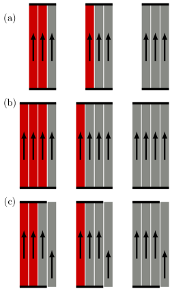
Figure 1: The models. (a): Three-lane closed systems with periodic boundary conditions (PBC) in the traveling direction; (b): Four-lane closed systems; (c): Four-lane open systems in which the right lane has two open ends and the other lanes have PBC. In each panel (a), (b) and (c) the figures from left to right correspond to the asymmetric model, the hybrid model and the symmetric model, respectively. The red lanes are overtaking lanes and the gray lanes are driving lanes.

Lane-changing rules in two-lane traffic are in general divided into two categories: symmetric and asymmetric Rickert ; Chowdhury . This classification can be generalized to models with more than two lanes. For example, a multilane system consisting entirely of driving lanes corresponds to a symmetric lane-changing model. An asymmetric lane-changing model in our program can be made up with a driving lane for the far right lane and overtaking lanes for all other lanes, or equivalently, it is constructed entirely with overtaking lanes (see Fig. 1). Here we also consider a case (a hybrid model) in which only the far left lane is the overtaking lane while the other lanes are driving lanes; this simple generalization, which differs from an asymmetric model when more than two lanes are considered, can be regarded as one minimal model that mimics highway rules implemented mainly outside of Europe, such as in the U.S. or in many countries of the Asia-Pacific region. We are not aware of any previous studies on the same hybrid model as we consider here.

Below we discuss our results for closed systems with periodic boundary conditions and for open systems with one open lane separately in two subsections.

III.1 Closed systems

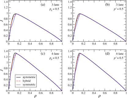
Figure 2: Fundamental diagrams for three-lane traffic (upper panel (a), (b)) and four-lane traffic (lower panel (c), (d)) on a road of length $L=1024$. The black, red and blue curves indicate data for the asymmetric, hybrid and symmetric lane change models, respectively. Two types of randomization in braking are considered: VDR type defined in Eq. (7) with $p_{0}=0.5$ (left panel) and a velocity-independent braking probability $p^{\prime}=0.5$ (right panel). The traffic flows for the three lane change models differ in the free-flow region, in which the flow for the asymmetric model is the highest, showing the advantage of this model over the other two models.

First we consider closed systems with two types of vehicles characterized by two different maximum forward velocities $v^{s}_{\rm max}=3(\rm{cells/time\;step})$ and $v^{f}_{\rm max}=5$, in which $25\%$ of the vehicles are of slow type. We focus on the case with velocity-dependent stochastic braking probabilities $p$:

$$p(v)=\begin{cases}0&{\rm for}\;v=v^{f}_{\rm max}\,,\\ p_{0}&{\rm for}\;v<v^{f}_{\rm max}\,.\end{cases}$$ (7)

This choice of $p(v)$ corresponds to the so-called ”cruise-control limit” in which fast vehicles at maximum allowed speed move deterministically Cruise . In the simulations performed, each density value for a system of length $L=1024$ was simulated using at least $T=50000$ time steps and the results were recorded after the first $10000$ steps. In addition, each data point is averaged over at least 100 samples.

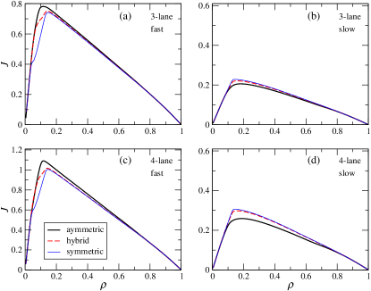
Figure 3: Flow-density diagrams for fast vehicles (subfigures (a), (c)) and slow vehicles (subfigures (b), (d)) in three different lane change models with velocity-dependent stochastic braking: $p_{0}=0.5$ for $v<v^{f}_{\rm max}$. The traffic flow of fast vehicles in the asymmetric model is overall highest, while the flow of slow vehicles in this model is lower than the other two models.

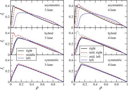
Figure 4: Flow-density diagrams for each lane in three-lane (left panel) and four-lane (right panel) traffic with the same simulation setup as in Fig. 3.

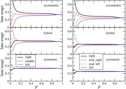
Figure 5: Lane usage for each lane in three-lane (left panel) and four-lane (right panel) traffic with the same simulation setup as in Fig. 3.

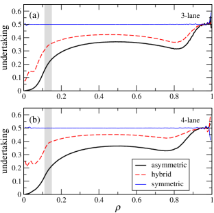
Figure 6: The fraction of undertaking in three-lane (a) and four-lane (b) traffic with the same simulation setup as in Fig. 3. The shaded area marks the densities of maximum flows in Fig. 2(a) and (c), i.e. the boundaries between a free-flow region and a jammed phase.

Fig. 2 shows the fundamental diagrams for flow($J$)-density($\rho$) relations in three- and four-lane traffic with three types of lane-changing rules, where results both for the VDR case with $p_{0}=0.5$ (see Eq. (7)) and for the case with a velocity-independent braking probability $p(v)=p^{\prime},\;\forall v$ are included. In all these cases, with increasing density one finds a transition from a free-flow region at low density into a jammed region at high density, separated by the peak of traffic flow. The diagrams suggest that different lane-changing rules have a stronger influence on the dynamics in the free-flow phase (close to the maximum of the flow) than in the jammed region; the asymmetric model, showing a higher flow in the free-flow phase, is the most efficient among three different lane-changing rules while the symmetric model is the least efficient. The advantage of the asymmetric model over the other two models with respect to traffic flow is mainly contributed by the fast vehicles, as we can see in Fig. 3. Slow vehicles, on the other hand, have lower average speed (i.e. smaller traffic flow at a given density) in the asymmetric model than the other two models.

In our program various quantities are measured also with respect to each lane. For example, Fig. 4 shows the flow-density relations for the individual lanes in three-lane and four-lane traffic for the VDR case with $p_{0}=0.5$. We notice that there are qualitative changes in the flow-density relations for certain lanes, such as the middle lane of the hybrid model, in which an inflection point appears on the right side of the flow maximum. The similar feature has been discussed in previous studies on metastable states in one-lane NaSch model with velocity dependent randomization VDR ; VDR1 .

Another interesting quantity for understanding effects of different lane-changing rules is the lane usage (defined as $N_{i}/N$ for the $i$-th lane), shown as a function of density in Fig. 5. We observe large occupancy of the right lane in the low-density regime (the free-flow region) of the asymmetric model and the right-lane usage remains higher than the other lanes when decreasing with growing density approaching $\rho\approx 0.9$, which reflects the Keep Right Unless Overtaking rule. In the hybrid model, the occupancy of the middle lane (or in the middle left lane in four-lane traffic) dominates at low densities, which is contributed by lane changes from the right side and also, in particular, from the leftmost passing lane as required by the rules; interestingly, there is a lane-usage inversion between two ”slow lanes” of the three-lane model when the density becomes larger than $\rho\approx 0.2$. Unlike the other models, the lane usage in the symmetric model is evenly distributed over all lanes except for a small enhancement in the middle lane(s) in the low-density limit. From the lane usage characteristic along with the flow-density diagrams of the individual lanes (Fig. 4), we summarize two observations as follows: (i) non-concavity occurs in the flow-density relation of the lane which exhibits a sharp decay of usage; (ii) the associated densities of the non-concavity region are those where the sharp decay of lane usage takes places.

Note that although the strategy of the asymmetric model implies a Keep Right Unless Overtaking rule, using the lane-changing criteria described in LC1-LC4 will not avoid ”undertaking” (i.e. passing on the right) in free traffic flow, which is prohibited by driving regulations in some countries. There are non-vanishing occurrences of undertaking for all $\rho>0$, as shown in Fig. 6. Nevertheless, the fraction of undertaking in the free-flow phase of the asymmetric model is considerably smaller than the fraction in the other two models. The increasing undertaking frequency at high densities reflects more symmetric lane usage in congested traffic.

III.2 Open systems

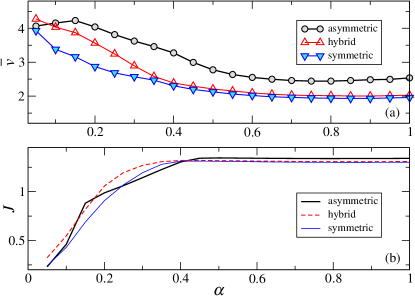
Figure 7: Average velocities (a) and flows (b) plotted against the entry rate in four-lane open systems. Three different lane-changing rules with velocity-dependent stochastic braking: $p_{0}=0.5$ for $v<v^{f}_{\rm max}$ are considered.

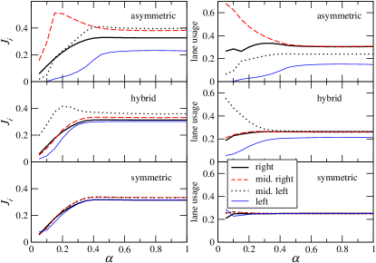
Figure 8: Flows (left panel) and lane usage (right panel) of the individual lanes in open systems with four lanes.

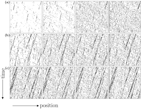
Figure 9: Space-time diagrams of four-lane open systems using $\alpha=0.95$ and $L=1024$. Panels (a), (b) and (c) are models with the asymmetric, hybrid and symmetric lane changing rules, respectively. From left to right: the left lane, the middle left lane, the middle right lane and the right lane with two open ends. In each model, 25% of vehicles entering the system are of slow type with a maximum allowed speed $v^{s}_{\rm max}=3$ and 75% of vehicles are of fast type with $v^{f}_{\rm max}=5$. In the figure, a black pixel represents a vehicle at a speed $v<5$ and white pixels are vacancies or vehicles at the highest speed $v=5$. The data were collected over the last 1024 time steps in total $10^{5}$ steps.

Now we turn to open systems. Here we consider systems which consist of a multilane part with periodic boundary conditions and a lane on the rightmost side with open ends, serving as on- and off-ramps (see Fig. 1(c)). It has been known for single-lane NaSch models that rules for injection and removal of vehicles have significant impacts on the traffic flow Open_NaSch ; Open_VDR ; Open_Ma ; Reentrance . Here for our multilane model we focus on the following strategies for vehicle injection and removal, that are incorporated into the single-lane updates and lane changes at each time step:

1. Injection strategy: With probability $\alpha$ a vehicle with initial velocity $v=1$ is inserted into site $j=0$ if the site is not occupied.

2. Removal strategy: If a vehicle moves out of the right lane from the open end at $j=L-1$ by the NaSch rules (A1-A4), we remove the vehicle with probability $\beta=1$.

The other parameters used for the simulation, such as types of vehicles and braking probabilities, are the same to the choices used for the closed systems; in particular, a VDR rule in the cruise-control limit (Eq. (7)) with $p_{0}=0.5$ for stochastic braking is applied, and two different values of the maximum allowed speed: $v^{s}_{\rm max}=3$ and $v^{f}_{\rm max}=5$ are assigned to vehicles that enter the system, in which $25\%$ of the vehicles are of slow type. We obtained observables at different entry rates ($\alpha$) and used more than $10^{5}$ time steps for each entry rate. The three types of lane-changing rules (asymmetric, hybrid and symmetric) discussed above are considered here too. For the asymmetric model, we set a default lane left adjacent to the open lane so that the criteria for changing back to the open lane are the same in all three models.

We graph average velocities and flows as functions of $\alpha$ for three different lane-changing models with four lanes in Fig. 7. In comparison, the velocity in the asymmetric model is overall higher, showing the advantage of the asymmetric lane-changing rules. All traffic flows saturate to constant values at high entry rates, where the flow of the asymmetric model is slightly larger than the other two models.

To analyze traffic behavior in each lane, in Fig. 8 we show simulation data for traffic flow and lane usage in the individual lanes, plotted against the entry rate. We observe that the flows in the lanes with high usage fraction (e.g. the middle right lane in the asymmetric model and the middle left lane in the hybrid model) exhibit non-monotonic behavior before they converge to constant values at larger $\alpha$; this is similar to what one observes in the flow-density diagrams of the closed systems shown in Fig. 4.

As a visual demonstration of the effects of lane-changing rules, typical space-time diagrams for the three different rules in the phase with $\alpha=0.95$ are shown in Fig. 9. The diagram for the asymmetric model shows small fluctuations in the two right lanes and low usage of the leftmost lane, while the plots for the hybrid and symmetric lane-changing rules exhibit traffic jams that persist for a long time in all lanes.

IV Summary and outlook

We have studied traffic flows on multilane highways with three different combinations of driving lanes and overtaking lanes. Lane-changing rules distinguish between a driving lane and an overtaking lane in the way that in a (middle) driving lane one makes lane changes to the left and to the right in symmetric manner, while in an overtaking lane vehicles obey asymmetric rules for lane changes. Using lane-changing criteria based on look-ahead distances we simulated three-lane and four-lane highway traffic in closed systems with periodic boundary conditions as well as in open systems with on- and off-ramps. Our results show that for heterogeneous traffic the asymmetric model with the rightmost lane as a driving lane and all the other lanes as overtaking lanes, which mimics the Keep Right Unless Overtaking rule, is more efficient than the other models in which lane-usage is almost equally distributed in all lanes.

We have developed an extensible software package for our study and make it publicly available for further applications. In addition to the observables considered in this paper, the code covers measurements of the order parameter, correlations, and relaxation time as defined in Ref. Relaxation ; Jamming , which makes it also useful for the study of jamming transitions and dynamic phase transitions in related models Autocorrelations ; Glass ; Finite ; Absorbing .

Author contribution statement

Y.C.L. devised the project. T.Z. developed the software package. Both T.Z. and Y.C.L performed the numerical simulations. Y.C.L. wrote the manuscript.

References

- (1) B. Derrida, M. R. Evans, V. Hakim, and V. Pasquier, J. Phys. A: Math. Gen. 26, 1493 (1993).
- (2) K. Nagel and M. Schreckenberg, J. Physique I 2, 2221 (1992).
- (3) D. Chowdhury, L. Santen, and A. Schadschneider, Physics Reports 329, 199 (2000).
- (4) K. Nagel, D. E. Wolf, P. Wagner, and P. Simon, Phys. Rev. E 58, 1425 (1998).
- (5) W. Knospe et al, J. Phys. A: Math. Gen. 35, 3369 (2002).
- (6) H. K. Lee, R. Barlovic, M. Schreckenberg, and D. Kim, Phys. Rev. Lett. 92, 238702 (2004).
- (7) L. Habel and M. Schreckenberg, in Cellular Automata, ACRI 2014. Lecture Notes in Computer Science, edited by J. Was, G. Ch. Sirakoulis, and S. Bandini, (Springer International Publishing, 2014), p. 620
- (8) Z. Su, W. Denga, L. Zhao, J. Han, W. Lib, and X. Cai, Eur. Phys. J. B 89, 203 (2016).
-
(9)
The software package is free available at:
http://www.iphys.nccu.edu.tw/Traffic/ - (10) R. Barlovic, L. Santen, A. Schadschneider, and M. Schreckenberg, Eur. Phys. J. B 5, 793 (1998).
- (11) M. Rickert, K. Nagel, M. Schreckenberg, and A. Latour, Physica A 231, 534 (1996).
- (12) D. Chowdhury, D. E. Wolf, and M. Schreckenberg, Physica A 235, 417 (1997).
- (13) K. Nagel and M. Paczuski, Phys. Rev. E 51, 2909 (1995).
- (14) S. Maerivoeta and B. De Moor, Eur. Phys. J. B 42, 131 (2004).
- (15) S. Cheybani, J. Kertész, and M. Schreckenberg, Phys. Rev. E 63, 016108 (2000).
- (16) R. Barlovic, T. Huisinga, A. Schadschneider, and M. Schreckenberg, Phys. Rev. E 66, 046113 (2002).
- (17) N. Jia and S. Ma, Phys. Rev. E 79, 031115 (2009); T. Neumann and P. Wagner, Phys. Rev. E 80, 013101 (2009); N. Zhu, S. Ma, and N. Jia, Phys. Rev. E 85, 043101 (2012).
- (18) M. Bouadi, K. Jetto, A. Benyoussef, A. El Kenz, Physica A 469, 1 (2017).
- (19) B. Eisenblaetter, L. Santen, A. Schadschneider, M. Schreckenberg, Phys. Rev. E 57, 1309 (1998).
- (20) G. Csányi, J. Kertész, J. Phys. A 28, L427 (1995).
- (21) J. de Gier, T. M. Garoni, and Z. Zhou, Phys. Rev. E 82, 021107 (2010).
- (22) A. S. de Wijn, D. M. Miedema, B. Nienhuis, and P. Schall, Phys. Rev. Lett. 109, 228001 (2012).
- (23) A. Balouchi and D. A. Browne, Phys. Rev. E 93, 052302 (2016).
- (24) M. L. L. Iannini and R. Dickman, Phys. Rev. E 95, 022106 (2017).