Mass composition of ultra-high-energy cosmic rays with the Telescope Array Surface Detector Data
Abstract
The results on ultra-high-energy cosmic rays (UHECR) mass composition obtained with the Telescope Array surface detector are presented. The analysis employs the boosted decision tree (BDT) multivariate analysis built upon 14 observables related to both the properties of the shower front and the lateral distribution function. The multivariate classifier is trained with Monte-Carlo sets of events induced by the primary protons and iron. An average atomic mass of UHECR is presented for energies . The average atomic mass of primary particles shows no significant energy dependence and corresponds to . The result is compared to the mass composition obtained by the Telescope Array with technique along with the results of other experiments. Possible systematic errors of the method are discussed.
I Introduction
The Telescope Array (TA) experiment is the largest ultra-high-energy (UHE) cosmic-ray experiment in the Northern hemisphere, located near Delta, Utah, USA Tokuno . TA is designed to register the extensive air showers (EAS) caused by the UHE cosmic rays entering the atmosphere. The experiment operates in hybrid mode and performs simultaneous measurements of the particle density and timing at the ground level with the surface detector array (SD) TASD and the fluorescence light with 38 fluorescence telescopes grouped into three fluorescence detector stations Tokuno2 . The SD is an array of 507 plastic scintillator detectors arranged on a square grid with 1.2 km spacing covering an area of approximately 700 . Each detector is composed of two layers of 1.2 cm thick extruded scintillator of the effective area.
There is a continuous progress of the experimental techniques, which started since the discovery of the cosmic rays more than a century ago. Recently, the results of three independent experiments confirmed the cut-off in the highest energy part HiresGZK ; AugerGZK ; TAGZK of the cosmic ray energy spectrum. The latter was predicted in 1966 by Greisen, Zatsepin and Kuzmin g ; zk . Still, the origin of the UHE cosmic rays remains unidentified. The mass composition of the UHE cosmic rays at Earth is one of the measurable quantities directly connected to the cosmic-ray acceleration mechanism in the source and source population as well as it is related to the propagation of the UHECR. Moreover, the mass composition is the main source of uncertainty in the expected cosmogenic photon and neutrino fluxes Gelmini:2005wu ; Aloisio:2015ega . In the wider scope, one needs the mass composition for precision tests of the Lorentz-invariance Saveliev and to ensure the safety of the future 100 TeV colliders. The latter is based on the constraints on the black hole production derived from the stability of dense astrophysical objects, such as white dwarfs and neutron stars, which interact with the cosmic rays. Black hole production rate depends on the the energy per nucleon and thus on the mass composition of the UHECR Sokolov:2016lba .
The most established method for the UHECR composition analysis is based on the measurements of the longitudinal shape of the EAS with the fluorescence telescope. This method uses the depth of the shower maximum as a composition-sensitive observable Gaisser:1993ix . There are UHE composition results available based on measured by the three experiments: HiRes, Pierre Auger Observatory and Telescope Array Abbasi2 ; Aab:2014aea ; Hanlon . The two latter results are compatible within the systematic errors in measurement which are of the order of in the energy range up to TA_AUGER_Composition_WG .
This Paper is dedicated to an alternative approach to measure the mass composition. The method uses solely the data of the surface detector which has an undoubted advantage of the longer than duty cycle TASD . Still, there is no single observable known that has a comparable to sensitivity to the mass composition, although measurements based on the risetime Aab:2016enk ; Aab:2017cgk have come close. In this Paper we use the multivariate boosted decision tree (BDT) Breiman ; Schapire technique based on a number of composition-sensitive variables obtained during the reconstruction of the SD events. The BDT method has proved itself reliable with a number of successful applications for the astroparticle physics experiments, see e.g. Krause ; Aab ; Abbasi .
The general scheme of the analysis is the following. The proton-induced and iron-induced Monte-Carlo events are simulated using the real-time calibration of the Telescope Array. The Monte-Carlo events are stored in the same format as the SD data and are split into three parts used in the following stages. First, a BDT classifier is trained using the first part of the proton-induced Monte-Carlo (MC) events as a background and iron-induced events as signal. Second, the distribution of the classifier output for data is compared to the second part of the proton and iron-induced MC events. The comparison results in the average atomic mass of the primary particle as a function of energy. Finally, the third part of the MC is used to estimate the bias of the method and to introduce a correction to in order to compensate it.
II Data set and simulations
II.1 Surface detector data
The data of the 9 years of the Telescope Array surface detector operation from May 11, 2008 to May 10, 2017 are used in this Paper. Each event is a set of the time-dependent signals (waveforms) from both upper and lower layers of each triggered station. The waveforms are recorded by the 12-bit flash analog-to-digital converters (FADC) with the 50 MHz sampling rate and are converted to MIPs TASD at the calibration stage. The station is marked as saturated at this stage if the saturation effects are significant. In the case of saturated detectors only the signal incidence time is used in the analysis.
II.2 Event reconstruction and cuts
Surface detector array event reconstruction is done in two steps TAGZK . At the first step, event geometry is reconstructed using the time of the arrival of the shower front particles measured by the triggered () counters. Shower front is approximated with empirical functions proposed by Linsley Linsley and later modified in AGASA experiment Teshima . Secondly, pulse heights in the counters together with the event geometry information are used for determining the normalization of the shower lateral distribution profile Takeda .
In order to determine the Linsley front curvature parameter an additional joint fit of shower front and lateral distribution function (LDF) is performed with 7 free parameters: , , , , , , TAgammalim :
| (1) |
| (2) |
| (3) |
| (4) |
where , , and are obtained from the pre-defined coordinate system of the array centered at the Central Laser Facility (CLF) Takahashi:2011zzd , is the delay of the shower plane and is the Linsley front curvature parameter. Including the Linsley front curvature, 14 composition-sensitive parameters are estimated for each event, see Appendix A for details.
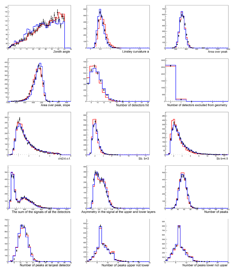
The parameters may be qualitatively split into three groups. The first group of parameters is related to the LDF which is known to be sensitive to . These are the for and Ros , the sum of the signals of all the detectors of the event, the number of the detectors hit and of the LDF fit.
The second group is related to the shower front which is in turn sensitive to both and the muon content of the shower. The Linsley curvature parameter designates the shower front curvature, while the area-over-peak of the signal, its slope and the number of detectors excluded from the fit correlate with the shower front width.
The latter group indicates the muon content of the shower. Muons cause the single peaks in FADC traces as they propagate rectilinearly and have small dispersion of arrival time. Moreover, muons induce identical signals in the upper and in the lower layers of the detector. Hence, the total number of peaks within all FADC traces, number of peaks in the detector with the largest signal, number of peaks present in the upper layer and not in the lower and vice versa, and also the asymmetry of the signal at the upper and at the lower layers of the detector are affected by the muonic component of the shower.
The following cuts are used to ensure the quality of reconstruction:
-
1.
event includes 7 or more triggered stations;
-
2.
zenith angle is below ;
-
3.
reconstructed core position inside the array with the distance of at least from the edge of the array;
-
4.
doesn’t exceed 4 for both the geometry and the LDF fits;
-
5.
doesn’t exceed 5 for the joint geometry and LDF fit.
-
6.
an arrival direction is reconstructed with accuracy less than ;
-
7.
fractional uncertainty of the is less than 25 %.
The same cuts are applied to both the data and the Monte-Carlo sets. The cuts listed above are tighter compared to the standard analysis cuts TAGZK due to the additional requirement of the curvature parameter reconstruction quality. Namely, 7 triggered stations is required instead of 5 and additional condition for the joint fit is included TAgammalim .
After the cuts, the SD data set contains 18068 events with energy greater than and less than .
BDT parameters distribution histograms for energy bin are denoted in Fig. 1, proton MC is shown with red lines, iron MC is shown with blue lines and black dots represent the data.
Let us discuss a contribution of individual parameters to overall BDT result. The TMVA package provides a relative importance value for each variable. The importance values are somewhat different in each energy range. Typically, the most discriminating variables are shower front curvature, and energy with importance about . The least discriminative variables are number of detectors hit and number of detectors excluded from geometry fit with importance about and correspondingly. The remaining 11 parameters have importance value between and .
II.3 Simulations
For the Monte-Carlo simulations, CORSIKA software package Heck is used along with the QGSJETII-03 model for high-energy hadronic interactions Ostapchenko , FLUKA FLUKA ; FLUKA2 for low energy hadronic interaction and EGS4 EGS4 for electromagnetic processes.
Due to the large number of particles born in an extensive air shower, modern computer resources available make it impractical to track every single one in a simulation. Instead, a thinning procedure was proposed Hillas . Within thinning, all particles with energies greater than a certain fraction of the primary energy are followed in detail, but below the threshold only one particle out of the secondaries produced in a certain interaction is randomly selected. This effective particle is assigned a weight to ensure energy conservation. The thinning level of with an additional weight limitation according to Kobal:2001jx is used for simulations. The thinning allows to achieve CPU-time efficiency, but at the same time introduces artificial statistical fluctuations Gorbunov:2007vj . The dethinning procedure is developed and implemented Stokes in order to restore the statistical properties of the shower. The detector response is simulated by the GEANT4 package Agostinelli . Real-time array status and detector calibration information for 9 years of observations are used for each simulated event TAdataMC . Two separate Monte-Carlo sets, for proton and iron primaries, are simulated and stored in the same data format as the SD data. In the energy range eV a set of 9800 CORSIKA showers was created. Using these showers, 200 million events were thrown on the detector for each MC set. The procedure of the Monte-Carlo set production for the Telescope Array is described in details in AbuZayyad:2012ru .
For each of the fourteen variables, its data and MC distributions were verified to be in the reasonable agreement. Within errors, all distributions of variables of data events lie between the proton and iron distributions.
III Method
III.1 BDT classifier
A number of composition-sensitive observables may be extracted from the data, and therefore one may benefit from using the multivariate analysis techniques. In this Paper, Boosted Decision Trees (BDT) technique is implemented, available as a part of the ROOT Toolkit for Multivariate Data Analysis (TMVA) package Hocker . The adaptive boosting (AdaBoost) algorithm is employed Schapire ; Freund with the number of trees NTrees=1000.
The proton and iron Monte-Carlo sets are split into 3 parts with equal statistics. The first part is used to build and train the BDT classifier based on 16 variables, including zenith angle, energy and 14 composition-sensitive parameters listed in Appendix A. Proton-induced MC showers are used as a background and iron-induced ones as a signal events. A separate classifier is constructed for each energy bin with the width of : last two bins were merged together due to low number of data events. The classifier is applied to the data set as well as to the two remaining parts of the Monte-Carlo sets.
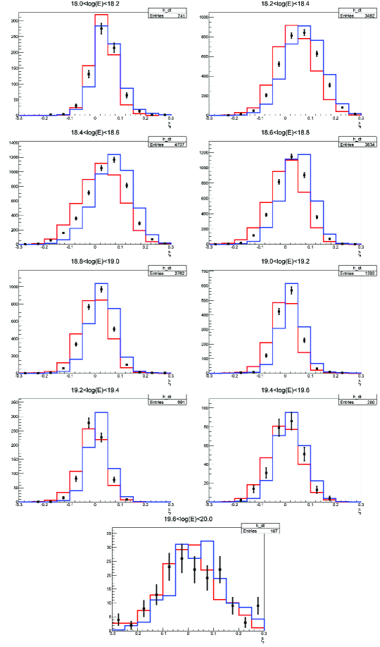
The result of the BDT classifier is a single value for each data and Monte-Carlo event. resides in the range , where is a pure signal event , – pure background event. The variable is used in the following one-dimensional analysis. Figure 2 shows parameter distribution histograms for all the energy bins, proton MC is shown with red lines, iron MC is shown with blue lines and black dots represent the data.
III.2 Estimation of an average atomic mass
Following the two-component approximation, the binned template fitting procedure is applied to , and data distributions separately in each energy bin. The implemented method is TFractionFitter ROOT package ROOT ; TFractionFitter . The second part of the Monte-Carlo is used in this step to obtain the fraction of proton and iron in the data, and , respectively.
The first estimate of an average atomic mass is based on the derived fraction of protons :
| (5) |
where and are average atomic masses of proton and iron nuclei.
We note that the number of proton and iron-induced simulated showers is the same, while the trigger and reconstruction efficiency differ. The proton fraction is defined as the fraction of proton simulated events in the mixture which corresponds to the hypothesis that is the average atomic mass of the particles arriving to the atmosphere. It is assumed that the detector efficiency affects the statistics of the proton and iron MC showers in the same way it affects the proton and iron-induced events in the data.
III.3 Bias correction
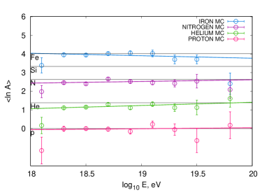
One may go further and build the bias correction procedure based on the Fig. 3. Assuming that the cosmic ray flux is composed of particles of single type in each energy bin, it is possible to construct the quadratic polynomial function based on obtained for four MC sets, for which the values are known.
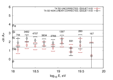
In the Figure 4 uncorrected and obtained with non-linear bias corrections are shown in comparison.
IV Results and discussion
IV.1 Estimation of the systematic error
The non-linear correction applied for the method is based on the assumption that the obtained composition is monotype. Thus the main source for the systematic error of the method is the inability to distinguish the mixture of a given elements and the single-type-particle composition.
To derive the systematic uncertainty, in each energy bin 100 mixtures of , , and Monte-Carlo sets were created, among which 50 mixtures are random monotype, 25 are random two-component and 25 are random four-component. Its values were estimated with the use of TFractionFitter template fitting method and non-linear bias corrections applied and compared with the “true” values calculated from the known fractions. Mean systematic error is estimated as:
| (6) |
IV.2 Hadronic models dependency
Composition results, both derived from surface detectors and in a hybrid mode, have a strong dependence on hadronic models used during Monte-Carlo simulations. Besides the one used in the above analysis, QGSJETII-04 Ostapchenko:2010vb , an improvement of QGSJETII-03 model, EPOS-LHC Pierog and SYBILL Fletcher models are also widely used.
All of the hadronic interaction models are based on the collider data and extrapolated to the UHECR energies. The analysis by the Pierre Auger Observatory has shown the inconsistency between muon signal predicted by simulations and data Aab:2016hkv . The same conclusions were also made based on the Telescope Array SD data Takeishi . This discrepancy may be the source of additional systematic bias which may affect the observables used for the composition study.
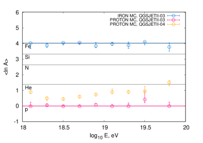
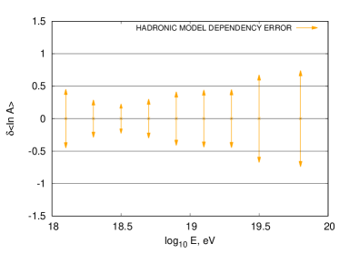
We study the systematic error introduced by the limited knowledge of the hadronic interaction models based on the comparison of the two models: QGSJETII-03 and QGSJETII-04 Ostapchenko:2010vb . For the latter, an additional proton Monte-Carlo set with the use of QGSJETII-04 model is simulated. The set is subjected to the same multivariate analysis procedure trained with the original QGSJETII-03 Monte-Carlo. The result is shown in the Fig. 5, while the hadronic model uncertainty as a function of energy is shown in Fig. 6. The uncertainty from hadronic interaction models is minimal at with and maximal at with .
IV.3 Composition
Mean logarithm of atomic mass as a function of energy without bias corrections and with the linear corrections applied is shown in Fig. 4. Within the errors, the average atomic mass of primary particles shows no significant energy dependence and corresponds to .
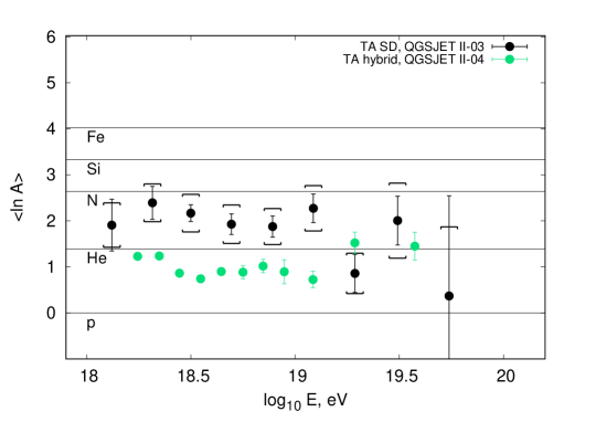
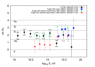
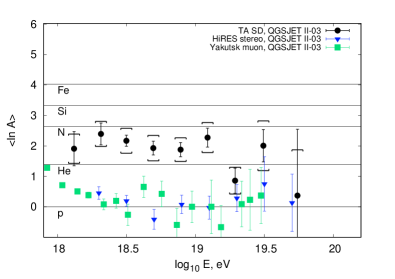
TA SD composition results in comparison with TA hybrid results are shown in Fig. 7. Comparisons with Pierre Auger Observatory SD based on muon density and muon arrival times and azimuthal risetime asymmetry, HiRes stereo and Yakutsk muon detector results are shown in Fig. 8 and 9, respectively. We mention that while there exist composition results based on the Pierre Auger Observatory hybrid observations Aab:2017njo , we focus only on the comparison with the corresponding surface detector results. The obtained composition is qualitatively consistent with the TA hybrid and the Pierre Auger Observatory results, while all the points lie higher than the pure proton composition observed by HiRes and Yakutsk.
Acknowledgment
The Telescope Array experiment is supported by the Japan Society for the Promotion of Science(JSPS) through Grants-in-Aid for Priority Area 431, for Specially Promoted Research JP21000002, for Scientific Research (S) JP19104006, for Specially Promote Research JP15H05693, for Scientific Research (S) JP15H05741 and for Young Scientists (A) JPH26707011; by the joint research program of the Institute for Cosmic Ray Research (ICRR), The University of Tokyo; by the U.S. National Science Foundation awards PHY-0601915, PHY-1404495, PHY-1404502, and PHY-1607727; by the National Research Foundation of Korea (2017K1A4A3015188 ; 2016R1A2B4014967; 2017R1A2A1A05071429, 2016R1A5A1013277); by IISN project No. 4.4502.13, and Belgian Science Policy under IUAP VII/37 (ULB). The development and application of the multivariate analysis method is supported by the Russian Science Foundation grant No. 17-72-20291 (INR). The foundations of Dr. Ezekiel R. and Edna Wattis Dumke, Willard L. Eccles, and George S. and Dolores Dore Eccles all helped with generous donations. The State of Utah supported the project through its Economic Development Board, and the University of Utah through the Office of the Vice President for Research. The experimental site became available through the cooperation of the Utah School and Institutional Trust Lands Administration (SITLA), U.S. Bureau of Land Management (BLM), and the U.S. Air Force. We appreciate the assistance of the State of Utah and Fillmore offices of the BLM in crafting the Plan of Development for the site. Patrick Shea assisted the collaboration with valuable advice on a variety of topics. The people and the officials of Millard County, Utah have been a source of steadfast and warm support for our work which we greatly appreciate. We are indebted to the Millard County Road Department for their efforts to maintain and clear the roads which get us to our sites. We gratefully acknowledge the contribution from the technical staffs of our home institutions. An allocation of computer time from the Center for High Performance Computing at the University of Utah is gratefully acknowledged. The cluster of the Theoretical Division of INR RAS was used for the numerical part of the work.
Appendix A: Composition-sensitive variables
In this work, a set of fourteen composition-sensitive variables is used:
-
Given a time resolved signal from a surface station, one may calculate its peak value and area, which are both well-measured and not much affected by fluctuations.
is fitted with a linear fit:
where m, is value at 1200 m and is its slope parameter.
-
4.
Number of detectors hit.
-
5.
Number of detectors excluded from the fit of the shower front by the reconstruction procedure AbuZayyad3 .
-
6.
of the joint geometry and LDF fit.
-
7–8.
parameter for and Ros . The definition of the parameter is the following:
where is the signal of i-th detector, is the distance from the shower core to this station in meters and – reference distance. The value and are used as they provide the best separation.
-
9.
The sum of the signals of all the detectors of the event.
-
10.
Asymmetry of the signal at the upper and lower layers of detectors.
-
11.
Total number of peaks within all FADC (flash analog-to-digital converter) traces.
This value is summed over both upper and lower layers of all stations of the event. To suppress accidental peaks resulting from FADC noise, the peak is defined as a time bin with a signal exceeding 0.2 vertical equivalent muons (VEM) with the value higher than signals of the 3 preceding and 3 consequent time bins.
-
12.
Number of peaks for the detector with the largest signal.
-
13.
Number of peaks present in the upper layer and not in the lower.
-
14.
Number of peaks present in the lower layer and not in the upper.
References
- (1) H. Tokuno et al. [Telescope Array Collaboration], J. Phys. Conf. Ser. 293, 012035 (2011).
- (2) T. Abu-Zayyad et al. [Telescope Array Collaboration], Nucl. Instrum. Meth. A 689, 87 (2013) [arXiv:1201.4964 [astro-ph.IM]].
- (3) H. Tokuno et al. [Telescope Array Collaboration], Nucl. Instrum. Meth. A 676, 54 (2012) [arXiv:1201.0002 [astro-ph.IM]].
- (4) R. U. Abbasi et al. [HiRes Collaboration], Phys. Rev. Lett. 100, 101101 (2008) & R. U. Abbasi et al. [HiRes Collaboration], Astropart. Phys. 32 (2010).
- (5) J. Abraham et al. [Pierre Auger Collaboration], Phys. Rev. Lett. 101, 061101 (2008) & J. Abraham et al. [Pierre Auger Collaboration], Phys. Lett. B 685 (2010).
- (6) T. Abu-Zayyad et al. [Telescope Array Collaboration], Astrophys. J. 768, L1 (2013) [arXiv:1205.5067 [astro-ph.HE]].
- (7) K. Greisen, Phys. Rev. Lett. 16, 748 (1966)
- (8) Z. T. Zatsepin and V. A. Kuz’min, Zh. Eksp. Teor. Fiz. Pis’ma Red. 4, 144 (1966)
- (9) G. Gelmini, O. E. Kalashev and D. V. Semikoz, J. Exp. Theor. Phys. 106, 1061 (2008) [astro-ph/0506128].
- (10) R. Aloisio, D. Boncioli, A. di Matteo, A. F. Grillo, S. Petrera and F. Salamida, JCAP 1510, no. 10, 006 (2015) [arXiv:1505.04020 [astro-ph.HE]].
- (11) A. Saveliev, L. Maccione and G. Sigl, JCAP 1103, 046 (2011) [arXiv:1101.2903 [astro-ph.HE]].
- (12) A. V. Sokolov and M. S. Pshirkov, arXiv:1611.04949 [hep-ph].
- (13) T. K. Gaisser et al., Phys. Rev. D 47, 1919 (1993).
- (14) R. U. Abbasi et al. [HiRes Collaboration], Phys. Rev. Lett. 104, 161101 (2010) [arXiv:0910.4184 [astro-ph.HE]].
- (15) A. Aab et al. [Pierre Auger Collaboration], Phys. Rev. D 90, no. 12, 122006 (2014) [arXiv:1409.5083 [astro-ph.HE]].
- (16) R. U. Abbasi et al. [Telescope Array Collaboration], Astrophys. J. 858, no. 2, 76 (2018) [arXiv:1801.09784 [astro-ph.HE]].
- (17) V. De Souza et al. Proceedings of the ICRC 2017, CRI167.
- (18) A. Aab et al. [Pierre Auger Collaboration], Phys. Rev. D 93, no. 7, 072006 (2016) [arXiv:1604.00978 [astro-ph.HE]].
- (19) A. Aab et al. [Pierre Auger Collaboration], Phys. Rev. D 96, no. 12, 122003 (2017) [arXiv:1710.07249 [astro-ph.HE]].
- (20) L. Breiman et al., Wadsworth International Group (1984).
- (21) R.E. Schapire, Mach. Learn. 5 (1990) 197.
- (22) M. Krause et al., Astropart. Phys. 89, 1 (2017) [arXiv:1701.06928 [astro-ph.IM]].
- (23) A. Aab et al. [Pierre Auger Collaboration], JCAP 1704 (2017) no.04, 009 [arXiv:1612.01517 [astro-ph.HE]].
- (24) R. Abbasi et al. [IceCube Collaboration], Phys. Rev. D 83 (2011) 012001 [arXiv:1010.3980 [astro-ph.HE]].
- (25) J. Linsley, L. Scarsi, Phys. Rev. 128 (1962) 2384.
- (26) M. Teshima et al., J. Phys. G 12, 1097 (1986).
- (27) M. Takeda et al., Astropart. Phys. 19, 447 (2003) [astro-ph/0209422].
- (28) T. Abu-Zayyad et al. [Telescope Array Collaboration], Phys. Rev. D 88, no. 11, 112005 (2013) [arXiv:1304.5614 [astro-ph.HE]].
- (29) Y. Takahashi et al. [Telescope Array Collaboration], AIP Conf. Proc. 1367, 157 (2011).
- (30) G. Ros et al., Astropart. Phys. 35, 140 (2011) [arXiv:1104.3399 [astro-ph.HE]].
- (31) D. Heck et al., Report FZKA-6019 (1998), Forschungszentrum Karlsruhe.
- (32) S. Ostapchenko, Nucl. Phys. Proc. Suppl. 151, 143 (2006) [hep-ph/0412332].
- (33) T. T. Böhlen et al., Nucl. Data Sheets 120, 211 (2014)
- (34) A. Ferrari, P. R. Sala, A. Fasso and J. Ranft, CERN-2005-010, SLAC-R-773, INFN-TC-05-11.
- (35) W. R. Nelson, H. Hirayama, D.W.O. Rogers, SLAC-0265 (permanently updated since 1985).
- (36) A. M. Hillas, Nucl. Phys. Proc. Suppl. 52B, 29 (1997).
- (37) M. Kobal [Pierre Auger Collaboration], Astropart. Phys. 15, 259 (2001).
- (38) D. S. Gorbunov, G. I. Rubtsov and S. V. Troitsky, Phys. Rev. D 76, 043004 (2007).
- (39) B. T. Stokes et al., Astropart. Phys. 35, 759 (2012).
- (40) S. Agostinelli et al. [GEANT4 Collaboration], Nucl. Instrum. Meth. A 506, 250 (2003).
- (41) T. Abu-Zayyad et al. [Telescope Array Collaboration], arXiv:1403.0644 [astro-ph.IM].
- (42) T. Abu-Zayyad et al. [Telescope Array Collaboration], Astrophys. J. 768, L1 (2013) [arXiv:1205.5067 [astro-ph.HE]].
- (43) A. Hocker et al., PoS ACAT (2007) 040 [physics/0703039 [PHYSICS]].
- (44) Y. Freund, R.E. Schapire, Proc. ICML (1996) 148.
- (45) R. Brun and F. Rademakers, Proceedings AIHENP’96 Workshop, Lausanne, Sep. 1996, Nucl. Inst. & Meth. in Phys. Res. A 389 (1997) 81-86, See also http://root.cern.ch/.
- (46) R. Barlow and C. Beeston, Comp. Phys. Comm. 77 (1993) 219-228.
- (47) S. Ostapchenko, Phys. Rev. D 83, 014018 (2011) [arXiv:1010.1869 [hep-ph]].
- (48) T. Pierog, I. Karpenko, J. M. Katzy, E. Yatsenko and K. Werner, Phys. Rev. C 92, no. 3, 034906 (2015) [arXiv:1306.0121 [hep-ph]].
- (49) R. S. Fletcher, T. K. Gaisser, P. Lipari and T. Stanev, Phys. Rev. D 50, 5710 (1994).
- (50) A. Aab et al. [Pierre Auger Collaboration], Phys. Rev. Lett. 117 (2016) no.19, 192001, [arXiv:1610.08509 [hep-ex]].
- (51) R. U. Abbasi et al. [Telescope Array Collaboration], Phys. Rev. D 98, no. 2, 022002 (2018) [arXiv:1804.03877 [astro-ph.HE]].
- (52) P. Abreu et al. [Pierre Auger Collaboration], Contributions to the 32nd International Cosmic Ray Conference, Beijing, China, August 2011 [arXiv:1107.4804 [astro-ph.HE]].
- (53) A. Sabourov et al., Contributions to the 35th International Cosmic Ray Conference, Busan, South Korea, July 2017, PoS(ICRC2017)553.
- (54) J. Bellido et al. [Pierre Auger Collaboration], PoS ICRC 2017 506, arXiv:1708.06592 [astro-ph.HE].
- (55) J. Abraham et al. [Pierre Auger Collaboration], Phys. Rev. Lett. 100, 211101 (2008) [arXiv:0712.1909 [astro-ph]].
- (56) T. Abu-Zayyad et al. [Telescope Array Collaboration], ApJL 768 (2013) L1.