Snapshot compressed sensing: performance bounds and algorithms

Abstract

Snapshot compressed sensing (CS) refers to compressive imaging systems in which multiple frames are mapped into a single measurement frame. Each pixel in the acquired frame is a noisy linear mapping of the corresponding pixels in the frames that are combined together. While the problem can be cast as a CS problem, due to the very special structure of the sensing matrix, standard CS theory cannot be employed to study such systems. In this paper, a compression-based framework is employed for theoretical analysis of snapshot CS systems. It is shown that this framework leads to two novel, computationally-efficient and theoretically-analyzable compression-based recovery algorithms. The proposed methods are iterative and employ compression codes to define and impose the structure of the desired signal. Theoretical convergence guarantees are derived for both algorithms. In the simulations, it is shown that, in the cases of both noise-free and noisy measurements, combining the proposed algorithms with a customized video compression code, designed to exploit nonlocal structures of video frames, significantly improves the state-of-the-art performance.

I Introduction

I-A Problem statement

The problem of compressed sensing (CS), recovering high-dimensional vector $\bm{x}\in\mathds{R}^{n}$ from its noisy under-determined linear measurements $\bm{y}=\bm{\Phi}\bm{x}+\bm{z}$, where $\bm{y},\bm{z}\in\mathds{R}^{m}$ and $\bm{\Phi}\in\mathds{R}^{m\times n}$, has been the subject of various theoretical and algorithmic studies in the past decade. Clearly, since such systems of linear equations are underdetermined, the recovery of $\bm{x}$ from measurements $\bm{y}$ is only feasible, if the input signal is structured. For various types of structure, such as sparsity, group-sparsity, etc., it is known that efficient algorithms exist that efficiently and robustly recover $\bm{x}$ from measurements $\bm{y}$. Starting by the seminal works of [2] and [3], there have been significant theoretical advances in this area. Initially, most such theoretical results were developed assuming that the entries of the sensing matrix $\bm{\Phi}$ are independently and identically distributed (i.i.d.) according to some distribution. In the meantime, various modern compressive imaging systems have been built during the last decade or so [4, 5, 6, 7, 8, 9] that are based on solving ill-posed linear inverse problems. Convincing results have been obtained in diverse applications, such as video CS [7, 8, 9] and hyper-spectral image CS [6, 10, 11]. However, except for the single-pixel camera [4] and similar architectures [12, 13], the sensing matrices employed in most of these practical systems are usually not random, and typically structured very differently compared to dense random sensing matrices studied in the CS literature. Therefore, more recently, there has also been significant effort on analyzing CS systems that employ structured sensing matrices. (Refer to [14, 15, 16, 17, 18, 19, 20] for some examples of such results.)

One important example of practical imaging systems built upon CS ideas is a hyperspectral compressive imaging system called coded aperture snapshot spectral imaging (CASSI)  [6]. CASSI recovers a three-dimensional (3D) spectral data cube, in which more than 30 frequency channels (images) at different wavelengths have been reconstructed, from a single two-dimensional (2D) captured measurement. This coded aperture modulating strategy has paved the way for many high-dimensional compressive imaging systems, from the aforementioned video CS to depth CS [21, 22], polarization CS [23], and joint temporal-spectral CS [24].

The measurement process in such hardware systems, known as snapshot CS systems, can typically be modeled as [8, 11]

$${\bm{y}={{\bf H}}\bm{x}+\bm{z}},$$ (1)

where, $\bm{x}\in\mathds{R}^{nB}$, and $\bm{y}\in\mathds{R}^{n}$ denote the desired signal, and the measurement vector, respectively. Here, $B$ denotes the number of $n$-dimensional input vectors (frames) that are combined together. In other words, the input $\bm{x}$ is a multi-frame signal that consists of $B$ $n$-dimensional vectors as

$$\bm{x}=\left[\begin{array}[]{c}\bm{x}_{1}\\ \vdots\\ \bm{x}_{B}\end{array}\right],$$ (2)

where $\bm{x}_{i}\in\mathds{R}^{n}$, $i=1,\ldots,B$. The measured signal is an $n$-dimensional vector. Thus, the sampling rate of this system is equal to ${n\over nB}={1\over B}$. The main difference between a standard CS system and a snapshot CS system lies in their sensing matrices. The sensing matrix ${{\bf H}}$ used in a snapshot CS system follows a very specific structure and can be written as

$${{{\bf H}}=\left[{\bf D}_{1},\dots,{\bf D}_{B}\right]},$$ (3)

where ${\bf D}_{k}\in\mathds{R}^{n\times n}$, $k=1,\ldots,B$, are diagonal matrices. It can be observed that, unlike dense matrices used in standard CS, here, the sensing matrix is very sparse. That is, of the $n^{2}B$ entries in matrix ${{\bf H}}$, at most, $nB$ of them are non-zero.

In this paper, we focus on and analyze such snapshot compressed sensing systems. As discussed before, a common property of such acquisition systems is that, due to some hardware constraints, each measurement only depends on few entries of the input signal. Furthermore, the location of the non-zero elements of the measurement kernel follows a very specific pattern. For example, in some video CS systems, high-speed frames are modulated at a higher frequency than the capture rate of the camera, which is working at a low frame rate. Each measured pixel in the captured frame is a function of the pixels located at the same position in the input frames. In this manner, each captured measurement frame can recover a number of high-speed frames, depending on the coding strategy, e.g., 148 frames are reconstructed from a snapshot measurement in [8].

In this paper, we provide the first theoretical analysis of snapshot CS systems and also propose new theoretically-analyzable robust recovery algorithms that achieve the state-of-the-art performance. As mentioned before, the main theoretical challenge is the fact that the sensing matrix is sparse and follows a very special structure.

I-B Contributions of this paper

As discussed in the last section, the main goal of our paper is to provide theoretical analysis for the snapshot CS system. More specifically, we aim to address the following fundamental questions regarding such systems:

• Is it theoretically possible to recover $\bm{x}$ from the measurement $\bm{y}$ defined in (1), for $B>1$?

• What is the maximum number of frames $B$ that can be mapped to a single measurement frame and still be recoverable, and how is this number related to the properties of the signal?

• Are there efficient and theoretically-analyzable recovery algorithms for snapshot CS?

Inspired by the idea of compression-based CS [25], we develop a theoretical framework for snapshot CS. We also propose two efficient iterative snapshot CS algorithms, called “compression-based PGD (CbPGD)” and “compression-based GAP (CbGAP)”, with convergence guarantees. The algorithms achieve state-of-the-art performance in snapshot video CS in our simulations. Though various algorithms, e.g. , [26, 27, 28], have been developed for video and hyper-spectral image CS, to our best knowledge, no theoretical guarantees have been available yet for the special structure of sensing matrices that arise in snapshot CS.

I-C Related work

As mentioned earlier, theoretical work in the CS literature is mainly focused on sparse signals [29, 3] and their extensions such as group-sparsity [30], model-based sparsity [31], and the low-rank property [32]. Many classes of signals such as natural images and videos typically follow much more complex patterns than these structures. A recovery algorithm that takes advantage of those complex structures, potentially, can outperform standard schemes by requiring a lower sampling rate or having a better reconstruction quality. However, designing and analyzing such recovery algorithms that impose both the measurement constraints and the source’s known patterns is in general very challenging. One recent approach to address this issue is to take advantage of algorithms that are designed for other data processing tasks such as denoising or data compression and to derive for instance denoising-based [33] or compression-based [25] recovery algorithms. The advantage of this approach is that, without much additional effort, it elevates the scope of structures used by CS recovery algorithms to those used by denoising or compression algorithms. As an example, modern image compression algorithms such as JPEG and JPEG2000 [34] are very efficient codes that are designed to exploit various common properties of natural images. Therefore, a CS recovery algorithm that employs JPEG2000 to impose structure on the recovered signal, ideally is a recovery algorithm that searches for a signal that is consistent with the measurements and at the same time satisfies the image properties used by the JPEG2000 code. This line of work of designing compression-based CS was first started in [25] and then later continued in [35], where the authors proposed an efficient compression-based recovery algorithm that achieves state-of-the-art performance in image CS.

Additionally, there are other CS systems such as those studied in [36, 13] for video CS, and [37] for hyperspectral imaging. (Please refer to the survey in [38, 39, 40] for more details on such systems.) While the sensing matrices used in these systems are not exactly as the sensing matrix defined in (3), they have key similarities, as in both cases they are very sparse in a very structured manner. Therefore, we expect that our proposed compression-based framework, with some moderate modifications, to be applicable to such cases as well and to pave the way for performing theoretical analysis of such systems too.

Finally, as mentioned in the introduction, the focus of this paper is on the imaging systems that can be approximated as a snapshot CS system. There are other types of imaging systems and CS systems with other types of constraints on the sensing matrices [14, 15, 16, 17, 18, 19, 20]. However, the sensing matrices considered therein are different from the one used in snapshot CS systems and hence those results are not applicable to such systems.

I-D Notation

Matrices are denoted by upper-case bold letters such as ${\bf X}$ and ${{\bf Y}}$. Vectors are denoted by bold lower-case letters, such as $\bm{x}$ and $\bm{y}$. For $\bm{x}\in\mathds{R}^{n}$ and $\bm{y}\in\mathds{R}^{n}$, $\langle\bm{x},\bm{y}\rangle=\sum_{i=1}^{n}x_{i}y_{i}$ denotes their inner product. Sets are denoted by calligraphic letters such as ${\cal X}$ and ${\cal Y}$. The size of a set ${\cal X}$ is denoted as $|\cal X|$. Throughout the paper, $\log$ and $\ln$ refer to logarithm in base 2 and natural logarithm, respectively.

I-E Paper organization

The rest of this paper is organized as follows. Section II briefly first reviews lossy compression codes for multi-frame signals and then develops and analyzes a compression-based snapshot CS recovery method. Section III introduces two different efficient compression-based recovery methods for snapshot CS, in subsections III-A and III-B and proves that they both converge. Simulation results of video CS are shown in Section IV. Section V provides proofs of the main results of the paper and Section VI concludes the paper.

II Data compression for snapshot CS

Our proposed framework studies snapshot CS systems via utilizing data compression codes. In the following, we first briefly review the definitions of lossy compression codes for multi-frame signals, and then develop our snapshot CS theory based on data compression.

II-A Data Compression

Consider a compact set ${\cal Q}\subset\mathbb{R}^{nB}$. Each signal ${\bm{x}}\in{\cal Q}$, consists of $B$ vectors (frames) $\{{\bm{x}}_{1},\ldots,{\bm{x}}_{B}\}$ in $\mathbb{R}^{n}$. A lossy compression code of rate $r$, $r\in\mathds{R}^{+}$ and can be larger than one, for ${\cal Q}$ is characterized by its encoding mapping $f$, where

$${f:{\cal Q}\rightarrow\{1,2,\ldots,2^{nBr}\},}$$ (4)

and its decoding mapping $g$, where

$${g:\{1,2,...,2^{nBr}\}\rightarrow\mathbb{R}^{nB}.}$$ (5)

The average distortion between ${\bm{x}}$ and its reconstruction $\hat{{\bm{x}}}$ is defined as

$${d({\bm{x}},\hat{{\bm{x}}})\triangleq{1\over nB}\sum_{i=1}^{B}{\left\|{{\bm{x}}_{i}-\hat{{\bm{x}}}_{i}}\right\|}_{2}^{2}={1\over nB}{\left\|{{\bm{x}}-\hat{{\bm{x}}}}\right\|}_{2}^{2}\;},$$ (6)

where ${\bm{x}}$ is defined in (2). Let $\tilde{\bm{x}}=g(f({\bm{x}})).$ The distortion of code $(f,g)$ is denoted by $\delta$, which is defined as the supremum of all achievable average per-frame distortions. That is,

$${\delta\triangleq\sup_{{\bm{x}}\in\mathcal{Q}}d({\bm{x}},\tilde{\bm{x}})=\sup_{{\bm{x}}\in\mathcal{Q}}{1\over nB}{\left\|{{\bm{x}}-\tilde{\bm{x}}}\right\|}_{2}^{2}.}$$ (7)

Let ${\cal C}$ denote the codebook of this code defined as

$${{\cal C}=\{g(f({\bm{x}})):\;{\bm{x}}\in\cal{Q}\}.}$$ (8)

Clearly, since the code is of rate $r$, $|{\cal C}|\leq 2^{nBr}$. Consider a family of compression code $\{(f_{r},g_{r})\}_{r}$ for set ${\cal Q}\subset\mathbb{R}^{nB}$, indexed by their rate $r$. The deterministic distortion-rate function of this family of codes is defined as

$$\delta(r)=\sup_{\bm{x}\in{\cal Q}}{1\over nB}\|\bm{x}-g_{r}(f_{r}(\bm{x}))\|_{2}^{2}.$$ (9)

The corresponding deterministic rate-distortion function of this family of codes is defined as

$${r(\delta)=\inf\{r:\delta(r)\leq\delta\}}.$$

The $\alpha$-dimension of this family of codes is defined as [25]

$${\alpha=\limsup_{\delta\to 0}{2r(\delta)\over\log{1\over\delta}}}.$$ (10)

It can be shown that in standard CS, the $\alpha$-dimension of a compression code is connected to the sampling rate required for a compression-based recovery method that employs this family of codes to, asymptotically, recover the input at zero distortion [25].

As an example, the set ${\cal Q}$ could represent the set of all $B$-frame natural videos and any video compression code, such as MPEG compression, could play the role of the compression code $(f,g)$.

In our theoretical derivations, to simplify the proofs, we make an additional assumption about the compression code as follows.

Assumption 1.

In our later theoretical derivations we assume that the compression code is such that $g(f(\bm{x}))$ returns the codeword in $\cal C$ that is closest to $\bm{x}$. That is, $g(f(\bm{x}))=\arg\!\min_{{\bm{c}}\in{\cal C}}\|\bm{x}-{\bm{c}}\|_{2}^{2}$.

The above assumption is not critical in our proofs and in fact it is straightforward to verify that relaxing this assumption only affects the reconstruction error by an additional term that is proportional to how well the mapping $g(f(\cdot))$ approximates the desired projection.

II-B Compression-based Recovery

While the main body of research in CS has focused on structures such as sparsity and its generalizations, recently, there has been a growing body work that consider much more general structures. Given the fact that most signals of interest follow structures beyond sparsity, such new schemes potentially are more efficient in terms of their required sampling rates or reconstruction quality.

One approach to develop recovery algorithms that employ more complex structures is to take advantage of already existing data compression codes. For some classes of signals such as images and videos, after decades of research, there exist efficient compression codes that take advantages of complex structures. Compressible signal pursuit (CSP), proposed in [25], is a compression-based recovery optimization. [25] shows that compression-based CS recovery is possible and can achieve the optimal performance in terms of required sampling rates.

Inspired by the CSP optimization, we propose a CSP-type optimization as a compression-based recovery algorithm for snapshot measurement systems. Consider the compact set ${\cal Q}\subset\mathbb{R}^{nB}$ equipped with a rate-$r$ compression code described by mappings $(f,g)$, defined in (4)-(5). Consider ${\bm{x}}\in\cal{Q}$ and its snapshot measurement

$${{\bm{y}}={{\bf H}}\bm{x}+\bm{z}=\sum_{i=1}^{B}{\bf D}_{i}{\bm{x}}_{i}+\bm{z},}$$ (11)

where ${{\bf H}}$ is defined in (3) and ${\bf D}_{i}=\mathrm{diag}(D_{i1},\ldots,D_{in})$. Then, a CSP-type recovery, given $\bm{y}$ and $({\bf D}_{1},\ldots,{\bf D}_{k})$, estimates $\bm{x}$ by solving the following optimization:

$${\hat{{\bm{x}}}=\arg\min_{{\bm{c}}\in{\cal C}}\|{\bm{y}}-\sum_{i=1}^{B}{\bf D}_{i}{\bm{c}}_{i}\|_{2}^{2},}$$ (12)

where ${\cal C}$ is defined in (8) and each codeword ${\bm{c}}$ is broken into $B$ $n$-dimensional blocks ${\bm{c}}_{1},\ldots,{\bm{c}}_{B}$ as (2). In other words, given a measurement vector $\bm{y}$, this optimization, among all compressible signals, i.e., signals in the codebook, picks the one that is closest to the observed measurements. As mentioned earlier, a key advantage of compression-based recovery methods such as (12) is that, without much additional effort, through the use of proper compression codes, they can take advantages of both temporal (spectral) and spatial dependencies that exist in multi-frame signals, such as videos. At $B=1$, with a traditional dense sensing matrix, this reduces to the standard CSP optimization [25]. However, theoretically, the two setups are significantly different, and for $B>1$, the original proof of the CSP optimization does not work in the snapshot CS setting.

The following theorem characterizes the performance of this CSP-type recovery method by connecting the parameters of the code, its rate and its distortion, to the number of frames $B$ and the reconstruction quality.

Theorem 1.

Assume that for all ${\bm{x}}\in{\cal Q}$, ${\left\|{{\bm{x}}}\right\|}_{\infty}\leq{\rho\over 2}$. Further consider a rate-$r$ compression code characterized by codebook $\cal C$ that achieves distortion $\delta$ on $\cal{Q}$. Moreover, ${\bf D}_{1},\ldots,{\bf D}_{B}$ are i.i.d., such that, for $i=1,\ldots,B$, ${\bf D}_{i}=\mathrm{diag}(D_{i1},\ldots,D_{in})$, and $\{D_{ij}\}_{j=1}^{n}\stackrel{{\scriptstyle\rm i.i.d.}}{{\sim}}{\cal N}(0,1)$. For $\bm{x}\in{\cal Q}$ and $\bm{y}=\sum_{i=1}^{B}{\bf D}_{i}{\bm{x}}_{i}$, let $\hat{\bm{x}}$ denote the solution of (12). Let $K=8/3$. Choose $\epsilon>0$, a free parameter, such that $\epsilon\leq 2K$. Then,

$${{1\over nB}\|{\bm{x}}-\hat{{\bm{x}}}\|_{2}^{2}\leq\delta+\rho^{2}\epsilon},$$ (13)

with a probability larger than ${1-2^{nBr+1}{\rm e}^{-{\epsilon^{2}n\over 16K^{2}}}}$.

The proof is presented in Section V-A.

Corollary 1.

Consider the same setup as in Theorem 1. Given $\eta>0$, assume that

$${B<{1\over\eta}({\log{1\over\delta}\over 2r}).}$$ (14)

Then,

$${\Pr\left({1\over nB}\|{\bm{x}}-\hat{{\bm{x}}}\|_{2}^{2}>\delta+{8\rho^{2}}\sqrt{\log{1\over\delta}\over\eta}\;\right)\leq 2{\rm e}^{-{\log{1\over\delta}\over 5\eta}n}}.$$ (15)

Proof.

In Theorem 1, let

$$\epsilon={8}\sqrt{\log{1\over\delta}\over\eta}.$$

Then, according to Theorem 1, the probability of the error event can be upper bounded by

$$2^{nBr+1}{\rm e}^{-{\epsilon^{2}n\over 16K^{2}}} \leq 2{\rm e}^{-{n\over\eta}\log{1\over\delta}\left({4\over K^{2}}-{\ln 2\over 2}\right)},$$ (16)

where $K=8/3$. But ${4\over K^{2}}-{\ln 2\over 2}>{1\over 5}$. Therefore, the desired result follows. ∎

Consider a family of compression codes $\{(f_{r},g_{r})\}_{r}$ for set ${\cal Q}\subset\mathbb{R}^{nB}$, indexed by their rate $r$. Roughly speaking, Corollary 1 states that, as $\delta\to 0$, if $B$ is smaller that $1\over\eta\alpha$, where $\alpha$ denotes the $\alpha$-dimension defined in (10), the achieved distortion by the CSP-type recovery is bounded by a constant that is inversely proportional to $1\over\sqrt{\eta}$. (Here, $\eta$ is a free parameter.) In snapshot CS, as mentioned earlier, the sampling rate is ${1\over B}$. Hence, in other words, to bound the achieved distortion, this corollary requires the sampling rate to exceed $\eta\alpha$.

To better understand the $\alpha$-dimension of structured multi-frame signals, inspired by video signals, consider the following set of $B$-frame signals in $\mathbb{R}^{nB}$. Assume that the first frame of each $B$-frame signal $\bm{x}\in{\cal Q}$ is an image that has a $k$-sparse representation. Further assume that the $\ell_{2}$-norm of $\bm{x}$ is bounded by $1$, i.e., $\|\bm{x}_{1}\|_{2}\leq 1$. Also assume that the next $(B-1)$ frames all share the same non-zero entries as $\bm{x}_{1}$ located arbitrarily across each frame. This very simple model is inspired by video frames and how consecutive frames are built by shifting the positions of the objects that are in the previous frames. Consider the following simple compression code for signals in $\cal Q$. For the first frame, we first use the orthonormal basis to transform the signal and then describe the locations of the (at most $k$) non-zero entries and their quantized values, each quantized into a fixed number of bits. Since, by our assumption, all frames share the same non-zero values, a code for all frames can be built by just coding the locations of the non-zero entries of the remaining $(B-1)$ frames. Changing the number of bits used to quantize each non-zero element yields a family of compression codes operating at different rates and distortions. Since the sparsifying basis is assumed be orthonormal, the $\alpha$-dimension of the code developed for the first frame $\bm{x}_{1}$ can be shown to be equal to ${k\over n}$ [25]. For the code developed for $B$-frame signals in $\cal Q$, since the number of bits required for describing the locations of the non-zero entries in each frame does not depend on the selected quantization level (or $\delta$), as $\delta\to 0$, the effect of these additional bits becomes negligible. Therefore, the $\alpha$-dimension of the family of codes designed for the described class of multi-frame signals is equal to $k\over nB$.

Finally, in Theorem 1, the measurements are assumed to be noise-free, which is not a realistic assumption. The following theorem shows the robustness of this method to bounded additive noise.

Theorem 2.

Consider the same setup as in Theorem 1. Assume that the measurements are corrupted by additive noise vector $\bm{z}$. That is, $\bm{y}=\sum_{i=1}^{B}{\bf D}_{i}{\bm{x}}_{i}+\bm{z}$, where $\bm{z}\in\mathds{R}^{n}$ denotes the measurement noise and ${1\over\sqrt{n}}{\left\|{\bm{z}}\right\|}_{2}\leq\sigma_{z}$, for some $\sigma_{z}\geq 0$. Let $\hat{\bm{x}}$ denote the solution of (12). Assume that $\epsilon>0$ is a free parameter such that $\epsilon\leq 2\sqrt{K}$, where $K=8/3$. Then,

$${1\over\sqrt{nB}}\|{\bm{x}}-\hat{{\bm{x}}}\|_{2}\leq{1\over\sqrt{nB}}\sqrt{\delta}+\rho\epsilon+{2\sigma_{z}\over\sqrt{B}},$$ (17)

with a probability larger than ${1-2^{nBr+1}{\rm e}^{-{\epsilon^{4}n\over 4^{3}K^{2}}}}$.

The proof is presented in Section V-B.

III Efficient compression-based snapshot CS

In the previous section we discussed a compression-based recovery method for snapshot compressed sensing which was inspired by the CSP optimization. Finding the solution of this optimization requires solving a high-dimensional non-convex discrete optimization, $\min_{{\bm{c}}\in{\cal C}}\|{\bm{y}}-\sum_{i=1}^{B}{\bf D}_{i}{\bm{c}}_{i}\|_{2}^{2}$. Solving this optimization involves minimizing a convex cost function over exponentially many codewords. Hence, finding the solution of the CSP optimization solution through exhaustive search over the codebook is infeasible, even for small values of blocklength $n$. To address this issue, in the following, we propose two different iterative algorithms for compression-based snapshot CS that are both computationally efficient, and both achieve good performances.

III-A Recovery Algorithm: Compression-based projected gradient descent

Projected gradient descent (PGD) is a well-established method for solving convex optimization problems and there have been extensive studies on the convergence performance of this algorithm [41]. More recent results, such as [42], also explore the performance of such algorithms when applied to non-convex problems different from those studied in this paper.

Inspired by PGD, Algorithm 1 described below is an iterative algorithm designed to approximate the solution of the non-convex optimization described in (12). Each iteration involves two key steps:

• moving in the direction of the gradient of the cost function,

• projecting the result onto the set of codewords.

Note that both steps are computationally very efficient. The gradient descent step involves matrix-vector multiplication, i.e., ${{\bf H}}\bm{x}^{t}$ and ${{\bf H}}^{\top}{\bm{e}}^{t}$ with ${\bm{e}}^{t}=\bm{y}-{{\bf H}}\bm{x}^{t}$ and ${{\bf H}}=[{\bf D}_{1},\ldots,{\bf D}_{B}]$. The second step, the projection on the set of codewords, can be performed by applying the encoder and the decoder of the compression code.

Algorithm 1 CbPGD for Snapshot CS recovery

0:  ${{\bf H}}$, $\bm{y}$.

1:  Initial $\mu>0$, $\bm{x}^{0}=0$.

2:  for $t=0$ to Max-Iter  do

3:     Calculate: ${\bm{e}}^{t}=\bm{y}-{{\bf H}}\bm{x}^{t}$.

4:     Projected gradient descent: ${\bm{s}}^{t+1}=\bm{x}^{t}+\mu{{\bf H}}^{\top}{\bm{e}}^{t}$.

5:     Projection via compression: $\bm{x}^{t+1}=g(f({\bm{s}}^{t+1}))$.

6:  end for

7:  Output: Reconstructed signal $\hat{\bm{x}}$.

The following theorem characterizes the performance of the proposed compression-based PGD (CbPGD) algorithm under the noiseless case, i.e., $\bm{z}=0$ in Eq. (11), and shows that if $B$ is small enough, Algorithm 1 converges.

Theorem 3.

Consider a compact set ${\cal Q}\subset\mathbb{R}^{nB}$, such that for all ${\bm{x}}\in{\cal Q}$, ${\left\|{{\bm{x}}}\right\|}_{\infty}\leq{\rho\over 2}$. Furthermore, consider a compression code for set ${\cal Q}$ with encoding and decoding mappings, $f$ and $g$, respectively. Assume that the code operates at rate $r$ and distortion $\delta$, and Assumption 1 holds. Consider ${\bm{x}}\in\cal{Q}$, and let $\tilde{{\bm{x}}}=g(f({\bm{x}}))$. Assume that ${\bm{x}}$ is measured as ${\bm{y}}=\sum_{i=1}^{B}{\bf D}_{i}{\bm{x}}_{i}$, where ${\bf D}_{i}=\mathrm{diag}(D_{i1},\ldots,D_{in})$, and $D_{ij}\stackrel{{\scriptstyle\rm i.i.d.}}{{\sim}}{\cal N}(0,1)$. Let $K=8/3$ and assume that $\delta\leq 2K\rho^{2}$. Set $\mu=1$, and let ${{\bm{x}}}^{t}$ denote the output of Algorithm 1 at iteration $t$. Then, given $\lambda\in(0,0.5)$, for $t=0,1,\ldots$, either ${1\over nB}{\left\|{\tilde{{\bm{x}}}-{{\bm{x}}}^{t}}\right\|}_{2}^{2}\leq\delta$, or

$${{1\over\sqrt{nB}}{\left\|{{{\bm{x}}}^{t+1}-\tilde{{\bm{x}}}}\right\|}_{2}\leq{2\lambda\over\sqrt{nB}}{\left\|{{{\bm{x}}}^{t}-\tilde{{\bm{x}}}}\right\|}_{2}+4\sqrt{\delta}},$$ (18)

with a probability at least

$${1-2^{4nBr}{\rm e}^{-({\delta\over 2K\rho^{2}})^{2}\lambda^{2}n}-(2^{2nBr}+1){\rm e}^{-n(\frac{\delta}{2K\rho^{2}})^{2}}}.$$ (19)

The proof is presented in Section V-C. The following direct corollary of Theorem 3 shows how for a bounded number of frames $B$, determined by the properties of the compression code, the algorithm converges with high probability.

Corollary 2.

Consider the same setup as Theorem 3. Given $\lambda\in(0,0.5)$ and $\epsilon>0$, assume that

$$B\leq{1+\epsilon\over 100r}({\delta\lambda\over\rho^{2}})^{2}.$$ (20)

Then, for $t=0,1,\ldots$, either ${1\over nB}{\left\|{\tilde{{\bm{x}}}-{{\bm{x}}}^{t}}\right\|}_{2}^{2}\leq\delta$, or

$${{1\over\sqrt{nB}}{\left\|{{{\bm{x}}}^{t+1}-\tilde{{\bm{x}}}}\right\|}_{2}\leq{2\lambda\over\sqrt{nB}}{\left\|{{{\bm{x}}}^{t}-\tilde{{\bm{x}}}}\right\|}_{2}+4\sqrt{\delta}},$$

with a probability larger than

$$1-{\rm e}^{-({3\delta\lambda\over 16\rho^{2}})^{2}\epsilon n}.$$ (21)

To better understand the convergence behavior of Theorem 3, the following corollary directly bounds the error at time $t$ as a function of the initial error and the distortion of the compression code.

Corollary 3.

Consider the same setup as Theorem 3. At iteration $t$, $t=0,1,\ldots,$, define the normalized error as

$$e_{t}\triangleq{1\over\sqrt{nB}}{\left\|{{{\bm{x}}}^{t}-\tilde{{\bm{x}}}}\right\|}_{2}.$$

Consider $\lambda\in(0,0.5)$, initialization point $\bm{x}^{0}$, and $\epsilon>0$. Assume that $B\leq{1+\epsilon\over 100r}({\delta\lambda\over\rho^{2}})^{2}$. Then at iteration $t$, either $e_{t^{\prime}}\leq\sqrt{\delta}$, for some $t^{\prime}\in\{1,\ldots,t\}$, or

$$e_{t+1}\leq(2\lambda)^{t+1}e_{0}+{4\over 1-2\lambda}\sqrt{\delta},$$

with a probability larger than $1-{\rm e}^{-({3\delta\lambda\over 16\rho^{2}})^{2}\epsilon n}$.

Next we consider the case where the measurements are corrupted by additive white Gaussian noise. The following theorem analyzes the convergence guarantee of the CbPGD algorithm in the case of noisy measurements and proves its robustness.

Theorem 4.

Consider the same setup as Theorem 3. Further assume that the measurements are corrupted by additive noise as

$${\bm{y}}=\sum_{i=1}^{B}{{\bf D}}_{i}{\bm{x}}_{i}+\bm{z},$$

where $\bm{z}\in\mathds{R}^{n}$ and $\{z_{i}\}_{i=1}^{n}\stackrel{{\scriptstyle i.i.d.}}{{\sim}}\mathcal{N}(0,\sigma^{2})$. Then, given $\lambda\in(0,0.5)$ and $\epsilon_{z}\in(0,\sqrt{\rho})$, for $t=0,1,\ldots$, either ${1\over nB}{\left\|{\tilde{{\bm{x}}}-{{\bm{x}}}^{t}}\right\|}_{2}^{2}\leq\delta$, or

$${1\over\sqrt{nB}}{\left\|{{{\bm{x}}}^{t+1}-\tilde{{\bm{x}}}}\right\|}_{2}\leq{2\lambda\over\sqrt{nB}}{\left\|{{{\bm{x}}}^{t}-\tilde{{\bm{x}}}}\right\|}_{2}+4\sqrt{\delta}+{2\epsilon_{z}\sigma\over\sqrt{B}},$$

with a probability larger than

$$1-2^{4nBr}{\rm e}^{-({{3\delta}\over{16\rho^{2}}})^{2}\lambda^{2}n} -(2^{2nBr}+1){\rm e}^{-n({{3\delta}\over{16\rho^{2}}})^{2}}-2^{2nBr}{\rm e}^{-n(\frac{3\epsilon_{z}}{16\rho})^{2}\delta}.$$ (22)

The proof is presented in Section V-D.

Remark 1.

The contribution of the measurement noise in Theorem 4 can be seen in two terms. First, there is an additional error term, ${2\epsilon_{z}\sigma\over\sqrt{B}}$, which is proportional to the power of the noise. Secondly, the term $2^{2nBr}{\rm e}^{-n(\frac{3\epsilon_{z}}{16\rho})^{2}\delta}$, which is part of the error probability, also depends on noise. In order to reduce the effect of noise, the first term suggests that we need to decrease the sampling rate, or equivalently increase $B$. This is of course counter-intuitive. However, note that this is happening because the non-zero entries of the sensing matrix are drawn i.i.d. $\mathcal{N}(0,1)$, and therefore the signal-to-noise ratio (SNR) per measurement is also proportional to $B$. To consider the more realistic situation, one can change the power of noise to $B\sigma^{2}$, i.e. fix the SNR with respect to $B$. Then, we see that the true effect of noise (in addition to increasing the reconstruction error) is revealed in $2^{2nBr}{\rm e}^{-n(\frac{3\epsilon_{z}}{16\rho})^{2}\delta}$. This term puts an extra upper bound on achievable $B$, the number of frames that can be combined together and later recovered.

III-B Compression-based generalized alternating projection

In the previous section we studied convergence performance of the CbPGD algorithm for a fixed $\mu$. However, in practice, as discussed later in Section IV, the step size $\mu$ needs to be optimized at each iteration. This optimization is usually time-consuming and hence noticeably increases the run time of the algorithm. In order to mitigate this issue, and due to the special structure of the sensing matrix, which makes ${{\bf H}}{{\bf H}}^{\top}$ a diagonal matrix, inspired by the generalized alternating projection (GAP) algorithm  [43], we propose a compression-based GAP (CbGAP) recovery algorithm for snapshot CS in Algorithm 2. Here, as before, ${{\bf H}}=[{\bf D}_{1},\ldots,{\bf D}_{B}]$, where ${\bf D}_{i}=\mathrm{diag}(D_{i1},\ldots,D_{in})$ denotes the sensing matrix. Matrix ${{\bf R}}$ is defined as

$${{{\bf R}}={{\bf H}}{{\bf H}}^{\top}={\rm diag}(R_{1},\dots,R_{n})},$$ (23)

where $R_{j}=\sum_{i=1}^{B}D^{2}_{ij},\forall j=1,\dots,n$. Note that the ${{\bf R}}^{-1}{\bm{e}}^{t}$ in the Euclidean projection step of Algorithm 2 can be computed element-wise and thus is very efficient. Moreover, during the implementation, we never store $\{{\bf D}_{i}\}_{i=1}^{B}$ and ${{\bf R}}$, but only their diagonal elements.

Algorithm 2 CbGAP for Snapshot CS recovery

0:  ${{\bf H}}$, $\bm{y}$.

1:  Initial $\mu>0$, $\bm{x}^{0}=0$.

2:  for $t=0$ to Max-Iter  do

3:     Calculate: ${\bm{e}}^{t}=\bm{y}-{{\bf H}}\bm{x}^{t}$.

4:     Euclidean projection: ${\bm{s}}^{t+1}=\bm{x}^{t}+\mu{{\bf H}}^{\top}{{\bf R}}^{-1}{\bm{e}}^{t}$.

5:     Projection via compression: $\bm{x}^{t+1}=g(f({\bm{s}}^{t+1}))$.

6:  end for

7:  Output: Reconstructed signal $\hat{\bm{x}}$.

The following theorem characterizes the convergence performance of the described compression-based GAP algorithm. Similar to Theorem 3, the following theorem proves that if $B$ is small enough, Algorithm 2 converges.

Theorem 5.

Consider the same setting as Theorem 3. For $t=0,1,\ldots$, let ${\bm{s}}^{t+1}=\bm{x}^{t}+B{{\bf H}}^{\top}{{\bf R}}^{-1}(\bm{y}-{{\bf H}}\bm{x}^{t}),$ and $\bm{x}^{t+1}=g(f({\bm{s}}^{t+1}))$, where ${{\bf R}}={{\bf H}}{{\bf H}}^{\top}$. Then, given $\lambda\in(0,0.5)$, for $t=0,1,\ldots$, either ${1\over nB}{\left\|{\tilde{{\bm{x}}}-{{\bm{x}}}^{t}}\right\|}_{2}^{2}\leq\delta$, or

$${{1\over\sqrt{nB}}\|{{\bm{x}}}^{t+1}-\tilde{{\bm{x}}}\|_{2}\leq{2\lambda\over\sqrt{nB}}{\left\|{{{\bm{x}}}^{t}-\tilde{{\bm{x}}}}\right\|}_{2}+4\sqrt{\delta}},$$

with a probability at least

$${1-2^{4nBr}{\rm e}^{-{\lambda^{2}\delta^{2}n\over 2B\rho^{4}}}-2^{2nBr}{\rm e}^{-{n\delta\over 2\rho^{2}B^{2}}}}.$$ (24)

The proof is presented in Section V-E. Note that, analogous to Corollary 3 of Theorem 3, Theorem 5 implies that ${1\over\sqrt{nB}}\|{{\bm{x}}}^{t+1}-\tilde{{\bm{x}}}\|_{2}$, for $B$ small enough, is bounded by ${(2\lambda)^{t+1}\over\sqrt{nB}}{\left\|{{{\bm{x}}}^{0}-\tilde{{\bm{x}}}}\right\|}_{2}+{4\over 1-2\lambda}\sqrt{\delta}$ with high probability

• Theorem 3 and Theorem 5 show that CbGAP and CbPGD have very similar convergence behaviors. Moreover, the important message of both results is the following: for a fixed $\lambda>0$, (19) and (24) bound the number of frames ($B$) that can be combined together, and still be recovered by the CbPGD algorithm and the CbGAP algorithm, respectively, as a function of $\lambda$, $\delta$, $r$, and $\rho$.

• Though Theorem 5 proves the convergence of GAP when $\mu=B$, in our simulations and in real applications, we found that $\mu\in\{1,2\}$ always leads to better results. By contrast, in CbPGD, $\mu=2/B$ is usually a good choice for a fixed step-size.

IV Simulation results

As mentioned earlier, snapshot CS is used in various applications. As a widely-used example, in this section, we report our simulation results for video CS and compare the performances of our proposed compression-based PGD and GAP algorithms with leading algorithms, i.e., GMM [26, 27], GAP-wavelet-tree [22], and GAP-TV [47]. For each method, we have used the codes provided by the authors on their websites. All algorithms are implemented in MATLAB.

Throughout the simulations, the pixel values are normalized into $[0,1]$, which corresponds to $\rho=2$ in our theorems. The standard peak-signal-to-noise-ratio (PSNR) is employed as the metric to compare different algorithms.

One key advantage of our proposed snapshot CS recovery algorithms is that they can readily be combined with any (off-the-shelf or newly-designed) compression codes. In the next sections, we first explore the performance of our proposed methods when MPEG coder  [48] is used as the video compression algorithm of choice. As shown in Section IV-A, this approach marginally improves the recovery performance compared to the existing methods. In Section IV-B, we propose employing a customized compression algorithm. Combining this compression code with our proposed compression-based recovery algorithms significantly improves the performance achieving a PSNR gain of 1.7 to 6 (dB), both in noiseless and noisy settings.

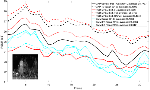
Figure 1: PSNR curves of reconstructed video frames compared with ground truth using different algorithms. $B=8$ with 4 measurements.

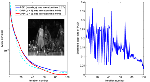
Figure 2: Left: The MSE of reconstructed video frames using GAP and PGD at each iteration. Right: The searched step size of PGD.

For Algorithm 1, Theorems 3 and 4 assume that $\mu$ is set to one. However, to speed up the convergence of the algorithm, in our simulations we adaptively choose the step size at each iteration, such that the measurement error is minimized after the projection step. Specifically, let $\mu_{t}$ denote the step-size at iteration $t$. Then, $\mu_{t}$ is set by solving the following optimization:

$$\mu_{t}=\arg\!\min_{\mu}\left\|\bm{y}-{{\bf H}}g\left(f(\bm{x}^{t}+\mu{{\bf H}}^{\top}(\bm{y}-{{\bf H}}\bm{x}^{t}))\right)\right\|_{2}.$$ (25)

This procedure attempts to move the next estimate as close as possible to the subspace of signals satisfying the measurement constraints, i.e., ${\cal M}=\{{\bm{\xi}}|\bm{y}={{\bf H}}{\bm{\xi}}\}$. We employ derivative-free methods, such as [49], to solve this optimization problem. However, this is still time-consuming. Unlike Algorithm 1, Algorithm 2 does not entail optimizing the step size and hence runs much faster.

IV-A MPEG Video Compression

In the first set of experiments we use the MPEG algorithm as the compression code required by the CbPGD algorithm (Algorithm 1) and the CbGAP algorithm (Algorithm 2). We refer to the resulting recovery methods as “PGD-MPEG” and “GAP-MPEG”, respectively. Fig. 1 plots the PSNR curves of different algorithms versus the frame number on the Kobe dataset used in [26]. Each video frame consists of $256\times 256$ pixels. $B=8$ video frames are modulated and collapsed into a single $256\times 256$ snapshot measurement. For the Kobe dataset, there are in total 32 frames and thus 4 measured frames are available. For each measured frame, given the masks, i.e., the sensing matrices $\{{\bf D}_{i}\}_{i=1}^{B}$, which are generated once and used in all algorithms, the task is to reconstruct the eight video frames. While the GMM-based algorithms are typically very slow, GAP-TV  [47] provides a decent result in a few seconds. Therefore, it is reasonable to initialize our PGD-MPEG and GAP-MPEG algorithms by the results of GAP-TV. It can be seen in Fig. 1 that after such initialization, the compression-based method outperforms other methods, but not with a significant margin.

Furthermore, note that both CbGAP and CbPGD algorithms are trying to approximate the solution of the non-convex optimization described in (12). On the other hand, our theorems do not guarantee convergence of either of the algorithms to the global optimal solution. Instead, our theoretical results guarantee that, with a high probability, each method convergences to a point that is in the close vicinity of the desired codeword. This is also confirmed by our simulation results. As seen in Fig. 1, regardless of the starting point, the PGD-MPEG algorithm converges and achieves a decent performance. However, changing the initialization point clearly affects the performance and a good initialization can noticeably improve the final result.

In Fig. 2, we plot the average per-pixel reconstruction mean square error (MSE) of (fixed step-size) GAP-MPEG and (step-size-optimized) PGD-MPEG, as the iterative algorithms proceed. It can be observed that after around 100 iterations GAP-MPEG and PGD-MPEG converge to similar levels of MSE. Moreover, the figure shows that setting $\mu=2$, GAP-MPEG outperforms both PGD-MPEG and GAP-MPEG with $\mu=1$. Since no step size search is required by GAP-MPEG, it runs much faster than PGD-MPEG. In fact, one iteration of GAP-MPEG on average takes about 0.09 seconds, which is 280 times faster than the time required by each iteration of PGD-MPEG. Through applying $\{R_{j}\}_{j=1}^{n}$, GAP-MPEG is applying a different step size to each measurement dimension, while PGD-MPEG on the other hand is trying to search for a fixed step size that works well for all measurement dimensions. The simulation results suggest that the former method while computationally more efficient achieves a better performance as well.

Finally, given that CbGAP achieves a similar or even better performance than CbPGD while running considerably faster, in the experiments done in the next section, we only report the performance results of the CbGAP algorithm.

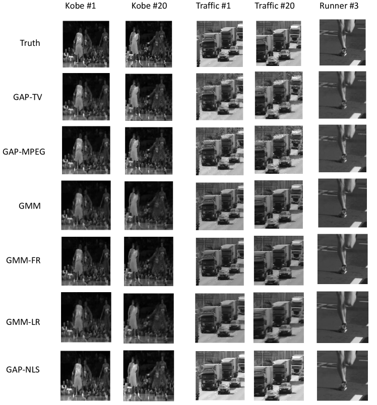
Figure 3: Reconstructed video frames of three datasets compared with group truth using different algorithms (shown on left).

IV-B Customized Video Compression

TABLE I: PSNR (dB) of reconstructed videos using different algorithms under noise-free measurements

Algorithm	Kobe	Traffic	Runner
GAP-TV [47]	26.47	20.17	30.05
GAP-wavelet-tree [22]	24.77	21.16	25.77
GMM [26]	23.71	21.03	29.03
GMM-FR [27]	23.44	21.84	33.16
GMM-LR [27]	23.91	21.09	30.70
GAP-MPEG	26.78	21.78	31.02
GAP-NLS	28.70	24.79	37.18

MPEG video compression involves performing two key steps: JPEG compression of the intra-frames (I-frames) and motion compensation, which exploits the temporal dependencies between different frames. One drawback of the JPEG-based MPEG compression is that, since it relies on discrete Cosine transformation (DCT) of individual local patches, it does not exploit nonlocal similarities [50] (The most recent video Codec, e.g., H.265/266 considers the similarities between patches but the patches need to be connected, thus it is still local similarity). Using nonlocal similarities in images or videos can potentially improve the performance significantly and this has been observed in various applications [51, 32, 52, 53].

As mentioned earlier, an advantage of compression-based recovery methods is that they can be combined with any appropriate compression code. Therefore, motivated by the discussed structures based on nonlocal similarities, we describe a compression code that takes advantage of such structures. Note that to employ a compression code within either of our algorithms, we only need to have access to the combined $g(f(\bm{x}))$ mapping, for any $\bm{x}\in\mathbb{R}^{nB}$, and not $f(\bm{x})$ itself. Hence, to describe our proposed compression code, we mainly focus on this mapping from input to its lossy reconstruction. The details of the code can be found in Appendix A. The key operation of the proposed code is the following: given a $B$-frame video $\{\bm{x}_{i}\}_{i=1}^{B}$ signal, using a small square window, it crawls over the first frame and considers all 3D blocks that result by considering the image of each block across the remaining $(B-1)$ frames. Then the similarities between these 3D blocks are measured and “similar” blocks are grouped together. After this, group-sparsity principles [54, 55] are used to encode such groups of blocks, which shares the same spirit with vBM4D [52].

Combining the described code with the CbGAP method (Algorithm 2) results in an algorithm which we refer to as “GAP-NLS” (GAP with nonlocal structure). To evaluate the performance of GAP-NLS, in addition to the Kobe dataset used above, we also consider the Traffic dataset used in [26] and the Runner dataset from [56]. Table I summarizes the video reconstruction results of our proposed method (GAP-NLS) compared with GAP-MPEG and other algorithms for these three videos. It can be observed that GAP-NLS achieves the best performance; It outperforms the best PSNR result achieved by other algorithms on Kobe, Traffic, and Runner datasets, by more than {2.2, 2.9, 4.0} (dB), respectively. The reconstructed video frames can be found in Fig. 3. Since the encoder here is more complicated than MPEG, each iteration costs about 3 seconds in our MATLAB implementation. Therefore, if a fast result is desired, GAP-MPEG is recommended and GAP-NLS is the best fit for high accuracy reconstructions.

TABLE II: PSNR (dB) of reconstructed videos using different algorithms under various noisy measurements

	Kobe			Traffic			Runner
Algorithm	$\sigma=0.01$	$\sigma=0.1$	$\sigma=0.5$	$\sigma=0.01$	$\sigma=0.1$	$\sigma=0.5$	$\sigma=0.01$	$\sigma=0.1$	$\sigma=0.5$
GAP-TV [47]	25.97	25.33	18.58	20.17	19.95	16.40	29.67	28.47	19.17
GAP-wavelet-tree [22]	23.77	24.19	18.12	21.15	20.91	16.85	25.61	23.76	19.16
GMM [26]	23.70	22.92	16.83	20.98	19.51	11.45	29.17	26.83	16.15
GAP-MPEG	26.78	25.53	19.69	21.77	21.10	17.05	30.91	28.30	21.06
GAP-NLS	28.61	27.04	20.64	24.56	23.98	18.54	34.57	30.80	22.00

IV-C Robustness to noise

So far, in all cases, the measurements were assumed to be noise-free. However, in real imaging systems, noise is inevitable. In this section, to further investigate the efficacy of our proposed algorithms, we perform the same experiments assuming that the measurements are corrupted by additive white Gaussian noise.

As mentioned earlier, the pixel values in the video are normalized into $[0,1]$. Gaussian noise is added to the measurements, as in  (11), where $\bm{z}\sim{\cal N}(0,\sigma^{2}{\bf I})$. Here $\sigma$ denotes the standard deviation of the Gaussian noise. Three different values of noise power have been studied, $\sigma=\{0.01,0.1,0.5\}$ corresponding to low, medium and high noise, respectively. Due to the extremely long running time of GMM-LR and GMM-FR, we hereby only compare with GAP-TV, GAP-wavelet-tree and GMM. The results are summarized in Table II. It can be observed that under small noises ($\sigma=0.01$), all algorithms work well. However, when the noise is getting larger, the algorithms show different behaviors. The GMM algorithm is affected by the noise severely when $\sigma=0.5$. This is due to the fact that GMM has a pre-defined noise value in GMM training and testing. However, in real cases, the noise value is unknown and the mismatch between the pre-defined value and real value will defeat the performance. In every case, our proposed GAP-NLS outperforms the other algorithms by at least 1.7 (dB) in PSNR. This clearly demonstrate the efficiency of our proposed algorithm.

Remark 2.

In our theoretical analysis, we assumed that we are given a compression code with a fixed rate. In practice, most compression codes have a parameter that sets their operating points in terms of rate and distortion. The choice of rate $r$ impacts the performance of the algorithm. In our simulations, we heuristically set the parameters of the compression code to optimize the performance, by sometimes changing it as the algorithm proceeds. In fact, we believe that one reason the customized compression code achieves better performance is that it provides more flexibility on choosing the quality parameter. Finding a theoretically-motivated approach to setting the parameters is an interesting problem that is left to future work.

V Proofs of the main results

Before presenting the proof, we first review some known results on the concentration of sub-Gaussian and sub-exponential random variables. These results are used throughout the proofs.

Definition 1.

A random variable $X$ is sub-Gaussian when

$${\left\|{X}\right\|}_{\psi_{2}}\triangleq\inf\Big{\{}L>0:{\rm E}\left[\exp\left(\frac{X^{2}}{L^{2}}\right)\right]\leq 2\Big{\}}<\infty.$$

Definition 2.

A random variable $X$ is a sub-exponential random variable, if

$${\left\|{X}\right\|}_{\psi_{1}}\triangleq\inf\Big{\{}L>0:{\rm E}\left[{\rm e}^{\frac{|X|}{L}}\right]\leq 2\Big{\}}<\infty.$$

Lemma 1.

For a normal random variable $X\sim\mathcal{N}(0,\sigma^{2})$, ${\left\|{X}\right\|}_{\psi_{2}}{}=\sqrt{8\over 3}\sigma$.

Proof.

Note that ${\rm E}\left[{\rm e}^{\frac{X^{2}}{L^{2}}}\right]=\int_{-\infty}^{\infty}(2\pi\sigma^{2})^{-0.5}{\rm e}^{-{x^{2}\over 2}({1\over\sigma^{2}}-{2\over L^{2}})}dx=\sqrt{L^{2}\over L^{2}-2\sigma^{2}}$, for $L>2\sigma^{2}$ and ${\rm E}\left[{\rm e}^{\frac{X^{2}}{L^{2}}}\right]=\infty$, otherwise. Moreover, ${\rm E}\left[{\rm e}^{\frac{X^{2}}{L^{2}}}\right]\leq 2$, as long as $3L^{2}\geq 8\sigma^{2}$. Hence, ${\left\|{X}\right\|}_{\psi_{2}}{}=\sqrt{8\over 3}\sigma$. ∎

Lemma 2.

If $X$ and $Y$ be sub-Gaussian random variables, then $XY$ is sub-exponential, and ${\left\|{XY}\right\|}_{\psi_{1}}\leq{\left\|{X}\right\|}_{\psi_{2}}{\left\|{Y}\right\|}_{\psi_{2}}.$

Proof.

Let $L={\left\|{XY}\right\|}_{\psi_{1}}$, $L_{1}={\left\|{X}\right\|}_{\psi_{2}}$ and $L_{2}={\left\|{Y}\right\|}_{\psi_{2}}$. To prove the desired result, we need to show that ${\rm E}\left[{\rm e}^{\frac{|XY|}{L_{1}L_{2}}}\right]\leq 2$. Since $\frac{|XY|}{L_{1}L_{2}}\leq{1\over 2}(\frac{X^{2}}{L_{1}^{2}}+\frac{Y^{2}}{L_{2}^{2}})$, ${\rm E}\left[{\rm e}^{\frac{|XY|}{L_{1}L_{2}}}\right]\leq{\rm E}\left[{\rm e}^{{1\over 2}(\frac{X^{2}}{L_{1}^{2}}+\frac{Y^{2}}{L_{2}^{2}})}\right]={\rm E}\left[{\rm e}^{\frac{X^{2}}{2L_{1}^{2}}}{\rm e}^{\frac{Y^{2}}{2L_{2}^{2}}}\right]\leq{1\over 2}{\rm E}\left[{\rm e}^{\frac{X^{2}}{L_{1}^{2}}}+{\rm e}^{\frac{Y^{2}}{L_{2}^{2}}}\right]\leq 2$. ∎

Theorem 6 (Bernstein Type Inequality, see e.g. [57]).

Consider independent random variables $\{X_{i}\}_{i=1}^{n}$, where for $i=1,\cdots,n$, $X_{i}$ is a sub-exponential random variable. Let $\max_{i}{\left\|{X_{i}}\right\|}_{\psi_{1}}\leq K$, for some $K>0$. Then for every $t\geq 0$ and every ${\bm{w}}=\left[w_{1},\cdots,w_{n}\right]^{T}\in\mathbbm{R}^{n\times 1}$, we have

$$\Pr\left(\sum_{i=1}^{n}w_{i}\left(X_{i}-{\rm E}\left[X_{i}\right]\right)\geq t\right)$$

$$\leq\exp\left\{-\min\left(\frac{t^{2}}{4K^{2}{\left\|{{\bm{w}}}\right\|}_{2}^{2}},\frac{t}{2K{\left\|{{\bm{w}}}\right\|}_{\infty}}\right)\right\}.$$ (26)

V-A Proof of Theorem 1

Proof.

Let $\tilde{{\bm{x}}}=g(f({\bm{x}}))$. By assumption the code operates at distortion $\delta$. Hence, ${1\over nB}{\left\|{{\bm{x}}-\tilde{{\bm{x}}}}\right\|}_{2}^{2}\leq\delta.$ Moreover, since $\hat{{\bm{x}}}=\arg\min_{{\bm{c}}\in{\cal C}}{\left\|{{\bm{y}}-\sum_{i=1}^{B}{\bf D}_{i}{\bm{c}}_{i}}\right\|}_{2}^{2}$ and $\tilde{{\bm{x}}}\in{\cal C}$, we have

$${\left\|{{\bm{y}}-\sum_{i=1}^{B}{\bf D}_{i}\hat{{\bm{x}}}_{i}}\right\|}_{2}^{2}\leq{\left\|{{\bm{y}}-\sum_{i=1}^{B}{\bf D}_{i}\tilde{{\bm{x}}}_{i}}\right\|}_{2}^{2},$$

or, since ${\bm{y}}=\sum_{i=1}^{B}{\bf D}_{i}{\bm{x}}_{i}$,

$${\left\|{\sum_{i=1}^{B}{\bf D}_{i}\left({\bm{x}}_{i}-\hat{{\bm{x}}}_{i}\right)}\right\|}_{2}^{2} \leq{\left\|{\sum_{i=1}^{B}{\bf D}_{i}\left({\bm{x}}_{i}-\tilde{{\bm{x}}}_{i}\right)}\right\|}_{2}^{2}.$$ (27)

Given $\epsilon_{1}>0$ and $\epsilon_{2}>0$ and ${\bm{x}}\in{\mathbb{R}}^{Bn}$, define events $\mathcal{E}_{1}$ and $\mathcal{E}_{2}$ as

$$\Big{\{} {1\over n}\Big{\|}\sum_{i=1}^{B}{\bf D}_{i}\left({\bm{x}}_{i}-{{\bm{c}}}_{i}\right)\Big{\|}_{2}^{2}\leq{1\over n}{\left\|{{\bm{x}}-{\bm{c}}}\right\|}_{2}^{2}+B\rho^{2}\epsilon_{1}:\forall{\bm{c}}\in\mathcal{C}\Big{\}}$$ (28)

and

$$\Big{\{}{1\over n}\Big{\|}\sum_{i=1}^{B}{\bf D}_{i}\left({\bm{x}}_{i}-{{\bm{c}}}_{i}\right)\Big{\|}_{2}^{2}\geq{1\over n}{\left\|{{\bm{x}}-{\bm{c}}}\right\|}_{2}^{2}-B\rho^{2}\epsilon_{2}:\forall{\bm{c}}\in\mathcal{C}\Big{\}},$$ (29)

respectively. Then, conditioned on $\mathcal{E}_{1}\cap\mathcal{E}_{2}$, since $\hat{{\bm{x}}}\in\mathcal{C}$ and $\tilde{{\bm{x}}}\in\mathcal{C}$, it follows from (27) that

$${1\over n}{\left\|{{\bm{x}}-\hat{{\bm{x}}}}\right\|}_{2}^{2}\leq{1\over n}{\left\|{{\bm{x}}-\tilde{{\bm{x}}}}\right\|}_{2}^{2}+B\rho^{2}\epsilon_{1}+B\rho^{2}\epsilon_{2}.$$ (30)

In the rest of the proof, we focus on bounding $P(\mathcal{E}_{1}^{c}\cup\mathcal{E}_{2}^{c})$. Note that, for a fixed ${\bm{c}}\in\mathcal{C}$,

$$\Big{\|}\sum_{i=1}^{B}{\bf D}_{i}\left({\bm{x}}_{i}-\tilde{{\bm{c}}}_{i}\right)\Big{\|}_{2}^{2} =\sum_{j=1}^{n}\left(\sum_{i=1}^{B}D_{ij}(x_{ij}-c_{ij})\right)^{2}.$$ (31)

Note that, for $j=1,\ldots,n$, $\sum_{i=1}^{B}D_{ij}\left(x_{ij}-c_{ij}\right)$ are independent zero-mean Gaussian random variables. Moreover,

$${\rm E}\left[\left(\sum_{i=1}^{B}D_{ij}(x_{ij}-c_{ij})\right)^{2}\right]$$

$$={\rm E}\left[\sum_{i=1}^{B}\sum_{i^{\prime}=1}^{B}D_{ij}D_{i^{\prime}j}(x_{ij}-c_{ij})(x_{i^{\prime}j}-c_{i^{\prime}j})\right]$$

$$=\sum_{i=1}^{B}(x_{ij}-c_{ij})^{2}.$$ (32)

For $j=1,\ldots,n$, define

$$w_{j}\triangleq\sum_{i=1}^{B}(x_{ij}-c_{ij})^{2},$$ (33)

and

$$Z_{j}\triangleq{\sum_{i=1}^{B}D_{ij}(x_{ij}-c_{ij})\over\sqrt{\sum_{i=1}^{B}(x_{ij}-c_{ij})^{2}}}.$$ (34)

Note that $Z_{1},\ldots,Z_{n}$ are i.i.d. $\mathcal{N}(0,1)$ random variables. Then, ${\left\|{\sum_{i=1}^{B}{\bf D}_{i}\left({\bm{x}}_{i}-{\bm{c}}_{i}\right)}\right\|}_{2}^{2}$ can be written as $\sum_{j=1}^{n}w_{j}Z^{2}_{j}$. But

$$\sum_{j=1}^{n}w_{j} =\sum_{j=1}^{n}\sum_{i=1}^{B}(x_{ij}-c_{ij})^{2}={\left\|{{\bm{x}}-{\bm{c}}}\right\|}_{2}^{2}.$$

Therefore, for a fixed ${\bm{c}}\in\mathcal{C}$,

$$\Pr \left({1\over n}{\left\|{\sum_{i=1}^{B}{\bf D}_{i}\left({\bm{x}}_{i}-{{\bm{c}}}_{i}\right)}\right\|}_{2}^{2}\geq{1\over n}\|{\bm{x}}-{\bm{c}}\|_{2}^{2}+B\rho^{2}\epsilon_{1}\right)$$

$$=\Pr\left({1\over n}\sum_{j=1}^{n}w_{j}(Z_{j}^{2}-1)\geq B\rho^{2}\epsilon_{1}\right),$$ (35)

where $w_{j}$ and $Z_{j}$ are defined in (33) and (34), respectively. As proved earlier, $Z_{1},\ldots,Z_{n}$ are i.i.d. $\mathcal{N}(0,1)$. Also, for all $j=1,\ldots,n$, ${\left\|{Z^{2}_{j}}\right\|}_{\psi_{1}}\leq{\left\|{Z_{j}}\right\|}_{\psi_{2}}^{2}\leq K$, where $K={8\over 3}$. Therefore, it follows from Theorem 6 that

$$\Pr \left({1\over n}{\left\|{\sum_{i=1}^{B}{\bf D}_{i}\left({\bm{x}}_{i}-{{\bm{c}}}_{i}\right)}\right\|}_{2}^{2}\geq{1\over n}{\left\|{{\bm{x}}-{\bm{c}}}\right\|}_{2}^{2}+B\rho^{2}\epsilon_{1}\right)$$

$$\leq\exp\left\{-\min\left(\frac{n^{2}B^{2}\rho^{4}\epsilon_{1}^{2}}{4K^{2}{\left\|{{\bm{w}}}\right\|}_{2}^{2}},\frac{nB\rho^{2}\epsilon_{1}}{2K{\left\|{{\bm{w}}}\right\|}_{\infty}}\right)\right\}.$$ (36)

Similarly, for fixed ${\bm{x}}$ and ${\bm{c}}$,

$$\Pr \left({1\over n}{\left\|{\sum_{i=1}^{B}{\bf D}_{i}\left({\bm{x}}_{i}-{{\bm{c}}}_{i}\right)}\right\|}_{2}^{2}\leq{1\over n}{\left\|{{\bm{x}}-{\bm{c}}}\right\|}_{2}^{2}-B\rho^{2}\epsilon_{2}\right)$$

$$\leq\exp\left\{-\min\left(\frac{n^{2}B^{2}\rho^{4}\epsilon_{2}^{2}}{4K^{2}{\left\|{{\bm{w}}}\right\|}_{2}^{2}},\frac{nB\rho^{2}\epsilon_{2}}{2K{\left\|{{\bm{w}}}\right\|}_{\infty}}\right)\right\}.$$ (37)

The final result follows by the union bound, and the fact that $|\mathcal{C}|\leq 2^{nBr}$. Note that ${\left\|{{\bm{w}}}\right\|}_{1}=\sum_{j=1}^{n}w_{j}=\sum_{j=1}^{n}\sum_{i=1}^{B}(x_{ij}-c_{ij})^{2}={\left\|{{\bm{x}}-{\bm{c}}}\right\|}_{2}^{2}$. Furthermore, since by assumption the $\ell_{\infty}$-norms of all signals in $\cal Q$ are upper-bounded by $\rho/2$, we have

$${\left\|{{\bm{w}}}\right\|}_{2}^{2} =\sum_{j=1}^{n}w_{j}^{2}=\sum_{j=1}^{n}\left(\sum_{i=1}^{B}(x_{ij}-c_{ij})^{2}\right)^{2}$$

$$\leq\sum_{j=1}^{n}\left(\sum_{i=1}^{B}\left({\rho\over 2}+{\rho\over 2}\right)^{2}\right)^{2}=B^{2}\rho^{4}n,$$ (38)

and

$${\left\|{{\bm{w}}}\right\|}_{\infty} =\max_{j=1\ldots,n}\sum_{i=1}^{B}(x_{ij}-c_{ij})^{2}\leq B\rho^{2}.$$ (39)

Therefore, combining (38) and (39) with (36) and (37), it follows that

$$\Pr \left({1\over n}{\left\|{\sum_{i=1}^{B}{\bf D}_{i}\left({\bm{x}}_{i}-{{\bm{c}}}_{i}\right)}\right\|}_{2}^{2}\geq{1\over n}{\left\|{{\bm{x}}-{\bm{c}}}\right\|}_{2}^{2}+B\rho^{2}\epsilon_{1}\right)$$

$$\leq\exp\Big{\{}-\min\left(\frac{n\epsilon_{1}^{2}}{4K^{2}},\frac{n\epsilon_{1}}{2K}\right)\Big{\}},$$ (40)

and

$$\Pr \left({1\over n}{\left\|{\sum_{i=1}^{B}{\bf D}_{i}\left({\bm{x}}_{i}-{{\bm{c}}}_{i}\right)}\right\|}_{2}^{2}\leq{1\over n}{\left\|{{\bm{x}}-{\bm{c}}}\right\|}_{2}^{2}-B\rho^{2}\epsilon_{2}\right)$$

$$\leq\exp\Big{\{}-\min\left(\frac{n\epsilon_{2}^{2}}{4K^{2}},\frac{n\epsilon_{2}}{2K}\right)\Big{\}},$$ (41)

respectively. Assume that $\max(\epsilon_{1},\epsilon_{2})\leq 2K$. Then, $\min\left(\frac{\epsilon_{1}}{2K},1\right)=\frac{\epsilon_{1}}{2K}$ and $\min\left(\frac{B\epsilon_{2}}{2K},1\right)=\frac{\epsilon_{2}}{2K}$. Hence,

$$\Pr \left({1\over n}{\left\|{\sum_{i=1}^{B}{\bf D}_{i}\left({\bm{x}}_{i}-{{\bm{c}}}_{i}\right)}\right\|}_{2}^{2}\geq{1\over n}{\left\|{{\bm{x}}-{\bm{c}}}\right\|}_{2}^{2}+B\rho^{2}\epsilon_{1}\right)$$

$$\leq\exp\Big{\{}-\frac{n\epsilon_{1}^{2}}{4K^{2}}\Big{\}},$$ (42)

and

$$\Pr \left({1\over n}{\left\|{\sum_{i=1}^{B}{\bf D}_{i}\left({\bm{x}}_{i}-{{\bm{c}}}_{i}\right)}\right\|}_{2}^{2}\leq{1\over n}{\left\|{{\bm{x}}-{\bm{c}}}\right\|}_{2}^{2}-B\rho^{2}\epsilon_{2}\right)$$

$$\leq\exp\Big{\{}-\frac{n\epsilon_{2}^{2}}{4K^{2}}\Big{\}}.$$ (43)

To finish the proof note that $|\mathcal{C}|\leq 2^{{nBr}}$. Therefore, by the union bound,

$$\Pr\left(\mathcal{E}_{1}^{c}\right)\leq 2^{nBr}\exp\Big{\{}-\frac{n\epsilon_{1}^{2}}{4K^{2}}\Big{\}},$$ (44)

and

$$\Pr\left(\mathcal{E}_{2}^{c}\right)\leq 2^{nBr}\exp\Big{\{}-\frac{n\epsilon_{2}^{2}}{4K^{2}}\Big{\}}.$$ (45)

Finally, again by the union bound, $P(\mathcal{E}_{1}\cap\mathcal{E}_{2})\geq 1-P(\mathcal{E}_{1}^{c})-P(\mathcal{E}_{2}^{c})$. Given $0<\epsilon<\frac{16}{3}$, the desired result follows by letting $\epsilon_{1}=\epsilon_{2}=\epsilon/2$. Plug this into (30), we have

$${1\over n}{\left\|{{\bm{x}}-\hat{{\bm{x}}}}\right\|}_{2}^{2}\leq{1\over n}{\left\|{{\bm{x}}-\tilde{{\bm{x}}}}\right\|}_{2}^{2}+B\rho^{2}\epsilon\leq B\delta+B\rho^{2}\epsilon.$$ (46)

This is

$${1\over nB}{\left\|{{\bm{x}}-\hat{{\bm{x}}}}\right\|}_{2}^{2}\leq\delta+\rho^{2}\epsilon.$$ (47)

Also, from (44) and (44), for $\epsilon_{1}=\epsilon_{2}=\epsilon/2$,

$$\Pr\left(\mathcal{E}_{1}\cap\mathcal{E}_{2}\right) \geq 1-2^{nBr}\exp\Big{\{}-\frac{n\epsilon_{1}^{2}}{4K^{2}}\Big{\}}-2^{nBr}\exp\Big{\{}-\frac{n\epsilon_{2}^{2}}{4K^{2}}\Big{\}}$$

$$=1-2^{nBr+1}\exp\Big{\{}-\frac{n\epsilon^{2}}{16K^{2}}\Big{\}}.$$ (48)

∎

V-B Proof of Theorem 2

Proof.

Similar to the proof of Theorem 1, let $\tilde{{\bm{x}}}=g(f({\bm{x}}))$. As before, ${1\over nB}{\left\|{{\bm{x}}-\tilde{{\bm{x}}}}\right\|}_{2}^{2}\leq\delta.$ Following the same initial steps as those used in the proof of Theorem 1, and noting that by the the triangle inequality, $\|\sum_{i=1}^{B}{\bf D}_{i}\left({\bm{x}}_{i}-\hat{{\bm{x}}}_{i}\right)+\bm{z}\|\geq\|\sum_{i=1}^{B}{\bf D}_{i}\left({\bm{x}}_{i}-\hat{{\bm{x}}}_{i}\right)\|-\|\bm{z}\|$ and $\|\sum_{i=1}^{B}{\bf D}_{i}\left({\bm{x}}_{i}-\tilde{{\bm{x}}}_{i}\right)+\bm{z}\|\leq\|\sum_{i=1}^{B}{\bf D}_{i}\left({\bm{x}}_{i}-\tilde{{\bm{x}}}_{i}\right)\|+\|\bm{z}\|$, we have

$${\left\|{\sum_{i=1}^{B}{\bf D}_{i}\left({\bm{x}}_{i}-\hat{{\bm{x}}}_{i}\right)}\right\|}_{2} \leq{\left\|{\sum_{i=1}^{B}{\bf D}_{i}\left({\bm{x}}_{i}-\tilde{{\bm{x}}}_{i}\right)}\right\|}_{2}+2{\left\|{\bm{z}}\right\|}_{2}.$$ (49)

Given $\epsilon_{1}>0$ and $\epsilon_{2}>0$ and ${\bm{x}}\in{\mathbb{R}}^{Bn}$, define events $\mathcal{E}_{1}$ and $\mathcal{E}_{2}$ as (28) and (29), respectively. Conditioned on $\mathcal{E}_{1}\cap\mathcal{E}_{2}$, since both $\hat{{\bm{x}}}$ and $\tilde{{\bm{x}}}$ are in the codebook of the code, it follows from (27) that

$$\sqrt{{\left\|{{\bm{x}}-\hat{{\bm{x}}}}\right\|}_{2}^{2}-nB\rho^{2}\epsilon_{2}}\leq\sqrt{{\left\|{{\bm{x}}-\tilde{{\bm{x}}}}\right\|}_{2}^{2}+nB\rho^{2}\epsilon_{1}}+2\|\bm{z}\|_{2}.$$ (50)

But, $\sqrt{a+b}\leq\sqrt{a}+\sqrt{b}$ and $\sqrt{a-b}\geq\sqrt{a}-\sqrt{b}$. Hence, from (50),

$${1\over\sqrt{nB}}{\left\|{{\bm{x}}-\hat{{\bm{x}}}}\right\|}_{2}-\sqrt{\rho^{2}\epsilon_{2}}\leq{1\over\sqrt{nB}}{\left\|{{\bm{x}}-\tilde{{\bm{x}}}}\right\|}_{2}+\sqrt{\rho^{2}\epsilon_{1}}+{2\|\bm{z}\|_{2}\over\sqrt{n}},$$

or

$${1\over\sqrt{nB}}{\left\|{{\bm{x}}-\hat{{\bm{x}}}}\right\|}_{2} \leq{1\over\sqrt{nB}}{\left\|{{\bm{x}}-\tilde{{\bm{x}}}}\right\|}_{2}+\rho(\sqrt{\epsilon_{1}}+\sqrt{\epsilon_{2}})+{2\|\bm{z}\|_{2}\over\sqrt{nB}}$$

$$\leq\sqrt{\delta}+\rho(\sqrt{\epsilon_{1}}+\sqrt{\epsilon_{2}})+{2\|\bm{z}\|_{2}\over\sqrt{nB}},$$

where the last line follows since the compression code operates at distortion $\delta$. Setting $\epsilon_{1}=\epsilon_{2}=\epsilon^{2}/4$, and noting that by assumption ${\|\bm{z}\|_{2}\over\sqrt{n}}\leq\sigma_{z}$, the desired result follows. Bounding $P(\mathcal{E}_{1}^{c}\cup\mathcal{E}_{2}^{c})$ can be done exactly as in the proof of Theorem 1.

∎

V-C Proof of Theorem 3

Proof.

Assume that ${1\over nB}{\left\|{\tilde{{\bm{x}}}-{{\bm{x}}}^{t}}\right\|}_{2}^{2}\leq\delta$ does not hold at iteration $t$. Then to prove the theorem, we need to show that eqrefeq:iterations-thm2 holds. At step $t$, given $\bm{x}^{t}$, define the error vector and its normalized version as

$$\bm{\theta}^{t}=\tilde{{\bm{x}}}-{{\bm{x}}}^{t},$$ (51)

and

$$\bar{{\bm{\theta}}}^{t}={{\bm{\theta}}^{t}\over{\left\|{{\bm{\theta}}^{t}}\right\|}_{2}},$$ (52)

respectively. By this definition, for $i=1,\ldots,B$, the $i$-th block of each of these error vectors can be written as ${\bm{e}}^{t}_{i}=\tilde{{\bm{x}}}_{i}-{{\bm{x}}}^{t}_{i}$, and

$$\bar{{\bm{\theta}}}^{t}_{i}={\tilde{{\bm{x}}}_{i}-{{\bm{x}}}^{t}_{i}\over{\left\|{\tilde{{\bm{x}}}-{\bm{x}}^{t}}\right\|}_{2}}.$$

Moreover, since by assumption ${1\over nB}{\left\|{\tilde{{\bm{x}}}-{{\bm{x}}}^{t}}\right\|}_{2}^{2}\geq\delta$,

$${1\over nB}\sum_{i=1}^{B}{\left\|{\tilde{{\bm{x}}}_{i}-{{\bm{x}}}_{i}^{t}}\right\|}_{2}^{2}\geq\delta,$$

Therefore, $\min\left({\left\|{{\bm{\theta}}^{t}}\right\|}_{2}^{2},{\left\|{{\bm{\theta}}^{t+1}}\right\|}_{2}^{2}\right)\geq nB\delta$.

For $i=1,\ldots,B$ and $j=1,\ldots,n$, since for all ${\bm{x}}\in{\cal Q}$, ${\left\|{{\bm{x}}}\right\|}_{\infty}\leq{\rho\over 2}$, we have

$$|\bar{\theta}^{t}_{ij}|^{2} ={(\tilde{{x}}_{ij}-{x}^{t}_{ij})^{2}\over{\left\|{{\bm{\theta}}^{t}}\right\|}_{2}^{2}}\leq{\rho^{2}\over nB\delta}$$ (53)

and, similarly,

$$|\bar{\theta}^{t+1}_{ij}|^{2}\leq{\rho^{2}\over nB\delta}$$ (54)

Since ${{\bm{x}}}^{t+1}$ is the closest codeword to ${\bm{s}}^{t+1}$ in $\mathcal{C}$, and $\tilde{{\bm{x}}}$ is also in $\mathcal{C}$, it follows that ${\left\|{{\bm{s}}^{t+1}-{{\bm{x}}}^{t+1}}\right\|}_{2}^{2}\leq{\left\|{{\bm{s}}^{t+1}-\tilde{{\bm{x}}}}\right\|}_{2}^{2},$ or

$$\sum_{i=1}^{B}{\left\|{{\bm{s}}_{i}^{t+1}-{{\bm{x}}}_{i}^{t+1}}\right\|}_{2}^{2}\leq\sum_{i=1}^{B}{\left\|{{\bm{s}}_{i}^{t+1}-\tilde{{\bm{x}}}_{i}}\right\|}_{2}^{2}.$$ (55)

But

$${\left\|{{\bm{s}}_{i}^{t+1}-{{\bm{x}}}_{i}^{t+1}}\right\|}_{2}^{2}={\left\|{{\bm{s}}_{i}^{t+1}-\tilde{{\bm{x}}}_{i}+\tilde{{\bm{x}}}_{i}-{{\bm{x}}}_{i}^{t+1}}\right\|}_{2}^{2}$$

$$={\left\|{{\bm{s}}_{i}^{t+1}-\tilde{{\bm{x}}}_{i}}\right\|}_{2}^{2}+2\left<{\bm{s}}_{i}^{t+1}-\tilde{{\bm{x}}}_{i},\tilde{{\bm{x}}}_{i}-{{\bm{x}}}_{i}^{t+1}\right>+{\left\|{\tilde{{\bm{x}}}_{i}-{{\bm{x}}}_{i}^{t+1}}\right\|}_{2}^{2}.$$ (56)

Therefore, along with (55),

$${\left\|{{\bm{s}}_{i}^{t+1}-\tilde{{\bm{x}}}_{i}}\right\|}_{2}^{2}+2\left<{\bm{s}}_{i}^{t+1}-\tilde{{\bm{x}}}_{i},\tilde{{\bm{x}}}_{i}-{{\bm{x}}}_{i}^{t+1}\right>+{\left\|{\tilde{{\bm{x}}}_{i}-{{\bm{x}}}_{i}^{t+1}}\right\|}_{2}^{2}$$

$$\leq{\left\|{{\bm{s}}_{i}^{t+1}-\tilde{{\bm{x}}}_{i}}\right\|}_{2}^{2}.$$ (57)

This is

$$\sum_{i=1}^{B}{\left\|{\tilde{{\bm{x}}}_{i}-{{\bm{x}}}_{i}^{t+1}}\right\|}_{2}^{2}\leq 2\sum_{i=1}^{B}\left<\tilde{{\bm{x}}}_{i}-{\bm{s}}_{i}^{t+1},\tilde{{\bm{x}}}_{i}-{{\bm{x}}}_{i}^{t+1}\right>$$

$$\stackrel{{\scriptstyle(a)}}{{=}}2\sum_{i=1}^{B}\left<\tilde{{\bm{x}}}_{i}-{{\bm{x}}}^{t}_{i}-{\bf D}_{i}{\bm{e}}^{t},\tilde{{\bm{x}}}_{i}-{{\bm{x}}}_{i}^{t+1}\right>$$

$$\stackrel{{\scriptstyle(b)}}{{=}}2\sum_{i=1}^{B}\left<\tilde{{\bm{x}}}_{i}-{{\bm{x}}}^{t}_{i},\tilde{{\bm{x}}}_{i}-{{\bm{x}}}_{i}^{t+1}\right>$$

$$\qquad-2\sum_{i=1}^{B}\left<{\bf D}_{i}\left({\bm{y}}-\sum_{j=1}^{B}{\bf D}_{j}{\bm{x}}_{j}^{t}\right),\tilde{{\bm{x}}}_{i}-{{\bm{x}}}_{i}^{t+1}\right>$$

$$=2\sum_{i=1}^{B}\left<\tilde{{\bm{x}}}_{i}-{{\bm{x}}}^{t}_{i},\tilde{{\bm{x}}}_{i}-{{\bm{x}}}_{i}^{t+1}\right>$$

$$\qquad-2\left<\sum_{j=1}^{B}{\bf D}_{j}\left({\bm{x}}_{j}-{\bm{x}}_{j}^{t}\right),\sum_{i=1}^{B}{\bf D}_{i}\left(\tilde{{\bm{x}}}_{i}-{{\bm{x}}}_{i}^{t+1}\right)\right>$$

$$=2\sum_{i=1}^{B}\left<\tilde{{\bm{x}}}_{i}-{{\bm{x}}}^{t}_{i},\tilde{{\bm{x}}}_{i}-{{\bm{x}}}_{i}^{t+1}\right>$$

$$\qquad-2\left<\sum_{i=1}^{B}{\bf D}_{i}\left({\bm{x}}_{i}-\tilde{{\bm{x}}}_{i}+\tilde{{\bm{x}}}_{i}-{\bm{x}}_{i}^{t}\right),\sum_{i=1}^{B}{\bf D}_{i}\left(\tilde{{\bm{x}}}_{i}-{{\bm{x}}}_{i}^{t+1}\right)\right>$$

$$=2\sum_{i=1}^{B}\left<\tilde{{\bm{x}}}_{i}-{{\bm{x}}}^{t}_{i},\tilde{{\bm{x}}}_{i}-{{\bm{x}}}_{i}^{t+1}\right>$$

$$\qquad-2\left<\sum_{i=1}^{B}{\bf D}_{i}\left(\tilde{{\bm{x}}}_{i}-{\bm{x}}_{i}^{t}\right),\sum_{i=1}^{B}{\bf D}_{i}\left(\tilde{{\bm{x}}}_{i}-{{\bm{x}}}_{i}^{t+1}\right)\right>$$

$$\qquad-2\left<\sum_{i=1}^{B}{\bf D}_{i}\left({\bm{x}}_{i}-\tilde{{\bm{x}}}_{i}\right),\sum_{i=1}^{B}{\bf D}_{i}\left(\tilde{{\bm{x}}}_{i}-{{\bm{x}}}_{i}^{t+1}\right)\right>.$$ (58)

where $(a)$ and $(b)$ follow from ${\bm{s}}^{t+1}_{i}=\bm{x}^{t}_{i}+{\bf D}_{i}{\bm{e}}^{t}$ and ${\bm{e}}^{t}=\bm{y}-\sum_{i=1}^{B}{\bf D}_{i}\bm{x}_{i}^{t}$, respectively. Then, using $\bar{{\bm{\theta}}}^{t}$ and $\bar{{\bm{\theta}}}^{t+1}$ defined in (52), the first two terms at the end of (58) can be written as

$$2\sum_{i=1}^{B}\left<\tilde{{\bm{x}}}_{i}-{{\bm{x}}}^{t}_{i},\tilde{{\bm{x}}}_{i}-{{\bm{x}}}_{i}^{t+1}\right>$$

$$\quad-2\left<\sum_{i=1}^{B}{\bf D}_{i}\left(\tilde{{\bm{x}}}_{i}-{\bm{x}}_{i}^{t}\right),\sum_{i=1}^{B}{\bf D}_{i}\left(\tilde{{\bm{x}}}_{i}-{{\bm{x}}}_{i}^{t+1}\right)\right>$$

$$= 2{\left\|{{\bm{\theta}}^{t}}\right\|}_{2}{\left\|{{\bm{\theta}}^{t+1}}\right\|}_{2}(\sum_{i=1}^{B}\left<\bar{{\bm{\theta}}}^{t}_{i},\bar{{\bm{\theta}}}_{i}^{t+1}\right>-\langle\sum_{i=1}^{B}{\bf D}_{i}\bar{{\bm{\theta}}}^{t}_{i},\sum_{i=1}^{B}{\bf D}_{i}\bar{{\bm{\theta}}}^{t+1}_{i}\rangle).$$ (59)

And

$$\sum_{i=1}^{B}\left<\bar{{\bm{\theta}}}^{t}_{i},\bar{{\bm{\theta}}}_{i}^{t+1}\right>-\left<\sum_{i=1}^{B}{\bf D}_{i}\bar{{\bm{\theta}}}^{t}_{i},\sum_{i=1}^{B}{\bf D}_{i}\bar{{\bm{\theta}}}^{t+1}_{i}\right>$$

$$=\sum_{j=1}^{n}\left(\sum_{i=1}^{B}\bar{\theta}^{t}_{ij}\bar{\theta}_{ij}^{t+1}-\left(\sum_{i_{1}=1}^{B}D_{i_{1}j}\bar{\theta}^{t}_{i_{1}j}\right)\left(\sum_{i_{2}=1}^{B}D_{i_{2}j}\bar{\theta}^{t+1}_{i_{2}j}\right)\right)$$

$$={1\over n}\sum_{j=1}^{n}\left(n\sum_{i=1}^{B}\bar{\theta}^{t}_{ij}\bar{\theta}_{ij}^{t+1}-U_{j}V_{j}\right),$$ (60)

where, for $j=1,\ldots,n$, random variables $U_{j}$ and $V_{j}$ are defined as

$$U_{j}\triangleq\sqrt{n}\sum_{i=1}^{B}D_{ij}\bar{\theta}^{t}_{ij},$$

and

$$V_{j}\triangleq\sqrt{n}\sum_{i=1}^{B}D_{ij}\bar{\theta}^{t+1}_{ij},$$

respectively.

Thus, Eq. (59), i.e., the first two terms of (58), becomes,

$$2\sum_{i=1}^{B}\left<\tilde{{\bm{x}}}_{i}-{{\bm{x}}}^{t}_{i},\tilde{{\bm{x}}}_{i}-{{\bm{x}}}_{i}^{t+1}\right>$$

$$\quad-2\left<\sum_{i=1}^{B}{\bf D}_{i}\left(\tilde{{\bm{x}}}_{i}-{\bm{x}}_{i}^{t}\right),\sum_{i=1}^{B}{\bf D}_{i}\left(\tilde{{\bm{x}}}_{i}-{{\bm{x}}}_{i}^{t+1}\right)\right>$$

$$=2{\left\|{{\bm{\theta}}^{t}}\right\|}_{2}{\left\|{{\bm{\theta}}^{t+1}}\right\|}_{2}{1\over n}\sum_{j=1}^{n}\left(n\sum_{i=1}^{B}\bar{\theta}^{t}_{ij}\bar{\theta}_{ij}^{t+1}-U_{j}V_{j}\right).$$ (61)

Impose the Cauchy-Schwarz inequality on the third term in (58), i.e.,

$$\left<\sum_{i=1}^{B}{\bf D}_{i}\left({\bm{x}}_{i}-\tilde{{\bm{x}}}_{i}\right),\sum_{i=1}^{B}{\bf D}_{i}\left(\tilde{{\bm{x}}}_{i}-{{\bm{x}}}_{i}^{t+1}\right)\right>$$

$$\leq\left\|\sum_{i=1}^{B}{\bf D}_{i}\left({\bm{x}}_{i}-\tilde{{\bm{x}}}_{i}\right)\right\|_{2}\left\|\sum_{i=1}^{B}{\bf D}_{i}\left(\tilde{{\bm{x}}}_{i}-{{\bm{x}}}_{i}^{t+1}\right)\right\|_{2}$$

$$=\left\|\sum_{i=1}^{B}{\bf D}_{i}\left({\bm{x}}_{i}-\tilde{{\bm{x}}}_{i}\right)\right\|_{2}\left\|\sum_{i=1}^{B}{\bf D}_{i}{\bm{\theta}_{i}^{t+1}}\right\|_{2}.$$ (62)

Now,  (58) becomes

$$\sum_{i=1}^{B}{\left\|{\tilde{{\bm{x}}}_{i}-{{\bm{x}}}_{i}^{t+1}}\right\|}_{2}^{2} \leq 2{\left\|{{\bm{\theta}}^{t}}\right\|}_{2}{\left\|{{\bm{\theta}}^{t+1}}\right\|}_{2}{1\over n}\sum_{j=1}^{n}\left(n\sum_{i=1}^{B}\bar{\theta}^{t}_{ij}\bar{\theta}_{ij}^{t+1}-U_{j}V_{j}\right)$$

$$\;\;+2\left\|\sum_{i=1}^{B}{\bf D}_{i}\left({\bm{x}}_{i}-\tilde{{\bm{x}}}_{i}\right)\right\|_{2}\left\|\sum_{i=1}^{B}{\bf D}_{i}{\bm{\theta}_{i}^{t+1}}\right\|_{2},$$ (63)

which is

$$\left\|\bm{\theta}^{t+1}\right\|_{2}^{2} \leq 2{\left\|{{\bm{\theta}}^{t}}\right\|}_{2}{\left\|{{\bm{\theta}}^{t+1}}\right\|}_{2}{1\over n}\sum_{j=1}^{n}\left(n\sum_{i=1}^{B}\bar{\theta}^{t}_{ij}\bar{\theta}_{ij}^{t+1}-U_{j}V_{j}\right)$$

$$\;\;+2\left\|\sum_{i=1}^{B}{\bf D}_{i}\left({\bm{x}}_{i}-\tilde{{\bm{x}}}_{i}\right)\right\|_{2}\left\|\sum_{i=1}^{B}{\bf D}_{i}{\bm{\theta}_{i}^{t+1}}\right\|_{2}.$$ (64)

Dividing both sides by $\|\bm{\theta}^{t+1}\|_{2}$,

$$\left\|\bm{\theta}^{t+1}\right\|_{2} \leq 2{\left\|{{\bm{\theta}}^{t}}\right\|}_{2}{1\over n}\sum_{j=1}^{n}\left(n\sum_{i=1}^{B}\bar{\theta}^{t}_{ij}\bar{\theta}_{ij}^{t+1}-U_{j}V_{j}\right)$$

$$\;\;+2\left\|\sum_{i=1}^{B}{\bf D}_{i}\left({\bm{x}}_{i}-\tilde{{\bm{x}}}_{i}\right)\right\|_{2}\left\|\sum_{i=1}^{B}{\bf D}_{i}{\bar{\bm{\theta}}_{i}^{t+1}}\right\|_{2}.$$ (65)

In the following, we first bound the first term in (65) using the Theorem 6.

• Bounds using Bernstein type inequality.

  Note that $(U_{j},V_{j})$, $j=1,\ldots,n$, are i.i.d. jointly Gaussian, such that

  $$U_{j}\sim\mathcal{N}\left(0,n\sum_{i=1}^{B}(\bar{\theta}^{t}_{ij})^{2}\right),$$

  $$V_{j}\sim\mathcal{N}\left(0,n\sum_{i=1}^{B}(\bar{\theta}^{t+1}_{ij})^{2}\right)$$

  and

  $${\rm E}\left[U_{j}V_{j}\right]=n\sum_{i=1}^{B}\bar{\theta}^{t}_{ij}\bar{\theta}_{ij}^{t+1}.$$

  By Lemma 2, since $U_{j}$ and $V_{j}$ are Gaussian random variables, $U_{j}V_{j}$ is a sub-exponential random variable and

  $${\left\|{U_{j}V_{j}}\right\|}_{\psi_{1}}\leq{8\over 3}n\sqrt{\sum_{i=1}^{B}(\bar{\theta}^{t}_{ij})^{2}\sum_{i=1}^{B}(\bar{\theta}^{t+1}_{ij})^{2}}.$$ (66)

  On the other hand, $(\bar{\theta}^{t}_{ij})^{2}$ and $(\bar{\theta}^{t+1}_{ij})^{2}$ are bounded as (53), i.e., $|\bar{\theta}^{t}_{ij}|^{2}\leq{\rho^{2}\over nB\delta},|\bar{\theta}^{t+1}_{ij}|^{2}\leq{\rho^{2}\over nB\delta}$ Therefore,

  $${\left\|{U_{j}V_{j}}\right\|}_{\psi_{1}} \leq{8\over 3}n\sum_{i=1}^{B}{\rho^{2}\over nB\delta}$$

  $$={8\rho^{2}\over 3\delta}$$

  $$={K\rho^{2}\over\delta},$$ (67)

  where $K=8/3$. Define the set of possible normalized error vectors of interest as follows

  $$\mathcal{F}\triangleq\Big{\{}{{\bm{c}}-{\bm{c}}^{\prime}\over{\left\|{{\bm{c}}-{\bm{c}}^{\prime}}\right\|}_{2}}:({\bm{c}},{\bm{c}}^{\prime})\in\mathcal{C}^{2},{\left\|{{\bm{c}}-{\bm{c}}^{\prime}}\right\|}_{2}\geq\sqrt{nB\delta}\Big{\}}.$$ (68)

  Employing Theorem 6 and (60), for a fixed $(\bar{{\bm{\theta}}},\bar{{\bm{\theta}}}^{\prime})\in\mathcal{F}^{2}$, we have

  $$\Pr \left(\sum_{j=1}^{n}\left(\sum_{i=1}^{B}\bar{\theta}_{ij}\bar{\theta}^{\prime}_{ij}-\left(\sum_{i=1}^{B}D_{ij}\bar{\theta}_{ij}\right)\left(\sum_{i=1}^{B}D_{ij}\bar{\theta}^{\prime}_{ij}\right)\right)\geq\epsilon\right)$$

  $$=\Pr\left({1\over n}\sum_{j=1}^{n}\left(n\sum_{i=1}^{B}\bar{\theta}_{ij}\bar{\theta}_{ij}-U_{j}V_{j}\right)\geq\epsilon\right)$$

  $$\leq\exp\Big{\{}-\min\left(\frac{n\epsilon^{2}}{4K^{2}},\frac{n\epsilon}{2K}\right)\Big{\}}$$

  $$=\exp\Big{\{}-\left(\frac{n\epsilon\delta}{2K\rho^{2}}\right)\min\left(\frac{\epsilon\delta}{2K\rho^{2}},1\right)\Big{\}}.$$ (69)

  where since $w_{j}=\frac{1}{n}$, $j=1,\ldots,n$, in Theorem 6, $\|\bm{w}\|_{2}^{2}=\|\bm{w}\|_{\infty}=1/n$. This leads to the final results in (69).

• Derive the union bound.

  Given $\lambda>0$, define event $\mathcal{E}_{1}$ as follows

  $$\mathcal{E}_{1}\triangleq\Big{\{}\sum_{j=1}^{n}\left(\sum_{i=1}^{B}\bar{\theta}_{ij}\bar{\theta}^{\prime}_{ij}-\left(\sum_{i=1}^{B}D_{ij}\bar{\theta}_{ij}\right)\left(\sum_{i=1}^{B}D_{ij}\bar{\theta}^{\prime}_{ij}\right)\right)$$

  $$\qquad\leq\lambda:\;\forall\;(\bar{{\bm{\theta}}},\bar{{\bm{\theta}}}^{\prime})\in\mathcal{F}^{2}\Big{\}}.$$ (70)

  Note the $\bar{\theta}_{ij}\bar{\theta}^{\prime}_{ij}$ in (70) is different and $\bar{\theta}_{ij}\bar{\theta}^{\prime}_{ij}$ in (69), where the one in (70) can be any value in a set $\mathcal{F}$, but the one in (69) is a fixed value.

  Let $\{\mathcal{E}_{i}^{c}\}_{i=1}^{3}$ denote the complementary event of $\mathcal{E}_{i}$, and we need to consider all values in the set $\mathcal{F}$. Combining the union bound with (69) yields

  $$\Pr\left(\mathcal{E}_{1}^{c}\right) \leq|\mathcal{F}|^{2}\exp\Big{\{}-\left(\frac{n\lambda\delta}{2K\rho^{2}}\right)\min\left(\frac{\lambda\delta}{2K\rho^{2}},1\right)\Big{\}}$$

  $$\leq 2^{4nBr}\exp\Big{\{}-\left(\frac{n\lambda\delta}{2K\rho^{2}}\right)\min\left(\frac{\lambda\delta}{2K\rho^{2}},1\right)\Big{\}},$$ (71)

  where the second step follows because $|\mathcal{F}|\leq|\mathcal{C}|^{2}\leq 2^{2nBr}$. Note that by assumption, $\delta\leq 16\rho^{2}/3$ and $0<\lambda<0.5$. Therefore,

  $${\frac{\lambda\delta}{2K\rho^{2}}=\frac{3\lambda\delta}{16\rho^{2}}\leq\lambda<1.}$$

  Therefore, (71) can be simplified as

  $$\Pr\left(\mathcal{E}_{1}^{c}\right) \leq 2^{4nBr}\exp\Big{\{}-\left(\delta\over 2K\rho^{2}\right)^{2}\lambda^{2}n\Big{\}}.$$ (72)

  Conditioned on $\mathcal{E}_{1}$, Eq. (65) becomes

  $${\left\|{{\bm{\theta}}^{t+1}}\right\|}_{2}\leq 2\lambda{\left\|{{\bm{\theta}}^{t}}\right\|}_{2}+2{\left\|{\sum_{i=1}^{B}{\bf D}_{i}\left({\bm{x}}_{i}-\tilde{{\bm{x}}}_{i}\right)}\right\|}_{2}{\left\|{\sum_{i=1}^{B}{\bf D}_{i}\bar{{\bm{\theta}}_{i}}^{t+1}}\right\|}_{2}$$ (73)

  For fixed $\bar{{\bm{\theta}}}=\bar{{\bm{\theta}}}^{\prime}$, (69) yields

  $$\Pr \left({\left\|{\sum_{i=1}^{B}{\bf D}_{i}\bar{{\bm{\theta}}_{i}}}\right\|}_{2}^{2}\leq 1-\epsilon\right)\leq\exp\Big{\{}-{\frac{n\epsilon^{2}\delta}{4K^{2}\rho^{2}}}\Big{\}}.$$ (74)

  Using the same procedure, we can derive a counterpart to the above bound as follows

  $$\Pr \left({\left\|{\sum_{i=1}^{B}{\bf D}_{i}\bar{{\bm{\theta}}_{i}}}\right\|}_{2}^{2}\geq 1+\epsilon\right)\leq\exp\Big{\{}-{\frac{n\epsilon^{2}\delta}{4K^{2}\rho^{2}}}\Big{\}}.$$ (75)

  Now we consider ${\left\|{\sum_{i=1}^{B}{\bf D}_{i}\left({\bm{x}}_{i}-\tilde{{\bm{x}}}_{i}\right)}\right\|}_{2}$ and ${\left\|{\sum_{i=1}^{B}{\bf D}_{i}\bar{{\bm{\theta}}_{i}}^{t+1}}\right\|}_{2}$ in (73) separately.

  • Given $\epsilon_{1}>0$, define event $\mathcal{E}_{2}$ as

    $$\mathcal{E}_{2}\triangleq\left\{{1\over n}{\left\|{\sum_{i=1}^{B}{\bf D}_{i}\left({\bm{x}}_{i}-\tilde{{\bm{x}}}_{i}\right)}\right\|}_{2}^{2}\leq{1\over n}{\left\|{{\bm{x}}-\tilde{{\bm{x}}}}\right\|}_{2}^{2}+B\rho^{2}\epsilon_{1}\right\}.$$ (76)

    Note that by the definition of $\delta$, we have

    $${\left\|{{\bm{x}}-\tilde{{\bm{x}}}}\right\|}_{2}^{2}\leq nB\delta.$$ (77)

    From (40), we have

    $$\Pr\left(\mathcal{E}_{2}^{c}\right)\leq\exp\Big{\{}-\min\left(\frac{n\epsilon_{1}^{2}}{4K^{2}},\frac{n\epsilon_{1}}{2K}\right)\Big{\}}.$$ (78)

    Conditioned on $\mathcal{E}_{2}$, we have

    $${\left\|{\sum_{i=1}^{B}{\bf D}_{i}\left({\bm{x}}_{i}-\tilde{{\bm{x}}}_{i}\right)}\right\|}_{2}^{2} \leq\|\bm{x}-\tilde{\bm{x}}\|_{2}^{2}+nB\rho^{2}\epsilon_{1}$$

    $$\leq nB\delta+nB\rho^{2}\epsilon_{1}$$

    $$=\sqrt{nB}\sqrt{\delta+\rho^{2}\epsilon_{1}}.$$ (79)

  • Given $\epsilon_{2}>0$, define event $\mathcal{E}_{3}$ as

    $$\mathcal{E}_{3}\triangleq\Big{\{}{\left\|{\sum_{i=1}^{B}{\bf D}_{i}\bar{{\bm{\theta}}_{i}}}\right\|}_{2}^{2}\leq 1+\epsilon_{2}:\;\forall\;{\bm{\theta}}\in\mathcal{F}\Big{\}}.$$ (80)

    Combining (75) with the union bound, we have

    $$\Pr\left(\mathcal{E}_{3}^{c}\right) \leq|\mathcal{F}|\exp\Big{\{}-{\frac{n\epsilon_{2}^{2}\delta}{4K^{2}\rho^{2}}}\Big{\}}\leq 2^{2nBr}\exp\Big{\{}-{\frac{n\epsilon_{2}^{2}\delta}{4K^{2}\rho^{2}}}\Big{\}}.$$ (81)

  Conditioned on $\mathcal{E}_{1}\cap\mathcal{E}_{2}\cap\mathcal{E}_{3}$, it follows from (73) that

  $${1\over\sqrt{nB}}{\left\|{{\bm{\theta}}^{t+1}}\right\|}_{2}\leq{2\lambda\over\sqrt{nB}}{\left\|{{\bm{\theta}}^{t}}\right\|}_{2}+2\sqrt{(1+\epsilon_{2})(\delta+\rho^{2}\epsilon_{1})}.$$ (82)

Combining (72), (78) and (81), it follows that

$$\Pr\left(\mathcal{E}_{1}\cap\mathcal{E}_{2}\cap\mathcal{E}_{3}\right) \geq 1-\sum_{i=1}^{3}\Pr\left(\mathcal{E}_{i}^{c}\right)$$

$$\geq 1-2^{4nBr}\exp\Big{\{}-\left(3\delta\over 16\rho^{2}\right)^{2}\lambda^{2}n\Big{\}}$$

$$\quad-\exp\Big{\{}-\min\left(\frac{n\epsilon_{1}^{2}}{4K^{2}},\frac{n\epsilon_{1}}{2K}\right)\Big{\}}-2^{2nBr}\exp\Big{\{}-{\frac{n\epsilon_{2}^{2}\delta^{2}}{4K^{2}\rho^{4}}}\Big{\}}.$$ (83)

Setting $\epsilon_{1}=\delta/\rho^{2}$ and $\epsilon_{2}=1$, it follows that

$$\min\left(\frac{n\epsilon_{1}^{2}}{4K^{2}},\frac{n\epsilon_{1}}{2K}\right) = \frac{n\delta}{2K\rho^{2}}\min\left(\frac{\delta}{2K\rho^{2}},1\right)$$ (84)

$$= n\left(\frac{\delta}{2K\rho^{2}}\right)^{2},$$ (85)

where the last line follows because $\delta\leq 2K\rho^{2}$ by assumption. Furthermore,

$$\frac{n\epsilon_{2}^{2}\delta^{2}}{4K^{2}\rho^{4}} = n\left(\frac{\delta}{2K\rho^{2}}\right)^{2}.$$ (86)

Hence, from (82), for $t=0,1,\ldots$,

$${1\over\sqrt{nB}}{\left\|{{\bm{\theta}}^{t+1}}\right\|}_{2}\leq{2\lambda\over\sqrt{nB}}{\left\|{{\bm{\theta}}^{t}}\right\|}_{2}+4\sqrt{\delta},$$ (87)

with a probability larger than

$$\Pr\left(\mathcal{E}_{1}\cap\mathcal{E}_{2}\cap\mathcal{E}_{3}\right) \geq 1-2^{4nBr}\exp\Big{\{}-n\left(\delta\lambda\over 2K\rho^{2}\right)^{2}n\Big{\}}$$

$$\qquad-(2^{2nBr}+1)\exp\left\{-n\left(\frac{\delta}{2K\rho^{2}}\right)^{2}\right\}.$$ (88)

∎

V-D Proof of Theorem 4

Proof.

Define the error vector and the normalized error vector as (51) and (52), respectively. Using the same procedure as the one used in deriving (58), and noting that unlike in (58), here, the measurements are noisy and ${\bm{y}}=\sum_{i=1}^{B}{\bf D}_{i}{\bm{x}}_{i}+\bm{z}$, it follows that

$$\sum_{i=1}^{B}{\left\|{{\bm{\theta}}_{i}^{k+1}}\right\|}_{2}^{2} \leq 2\sum_{i=1}^{B}\left<{\bm{\theta}}_{i}^{k+1},{\bm{\theta}}_{i}^{k}\right>-2\left<\sum_{i=1}^{B}{\bf D}_{i}{\bm{\theta}}_{i}^{k},\sum_{i=1}^{B}{\bf D}_{i}{\bm{\theta}}_{i}^{k+1}\right>$$

$$\;\;-2\left<\sum_{i=1}^{B}{\bf D}_{i}\left({\bm{x}}_{i}-\tilde{{\bm{x}}}_{i}\right),\sum_{i=1}^{B}{\bf D}_{i}{\bm{\theta}}^{k+1}\right>$$

$$\;\;+2\left|\sum_{i=1}^{B}\left<{\bf D}_{i}\bm{z},{\bm{\theta}}_{i}^{k+1}\right>\right|.$$ (89)

Define the set of all possible normalized error vectors $\mathcal{F}$ as in (68). Then, given $\lambda>0$, $\epsilon_{1}>0$ and $\epsilon_{2}>0$, define events $\mathcal{E}_{1}$ $\mathcal{E}_{2}$ and $\mathcal{E}_{3}$ as (70), (76) and (80), respectively. Conditioned on $\mathcal{E}_{1}\cap\mathcal{E}_{2}\cap\mathcal{E}_{3}$, using (82), (89) and setting $\epsilon_{1}$ and $\epsilon_{2}$ as before, it follow that

$${\left\|{{\bm{\theta}}^{k+1}}\right\|}_{2} \leq 2\lambda{\left\|{{\bm{\theta}}^{k}}\right\|}_{2}+4\sqrt{nB\delta}+2\left|\sum_{i=1}^{B}\left<{\bf D}_{i}\bm{z},\bar{{\bm{\theta}}}_{i}^{k+1}\right>\right|.$$ (90)

To finish the proof we need to bound $\left|\sum_{i=1}^{B}\left<{\bf D}_{i}\bm{z},\bar{{\bm{\theta}}}_{i}^{k+1}\right>\right|$. To achieve this goal, given $\epsilon_{z}\in(0,\sqrt{\rho})$, define event $\mathcal{E}_{z}$ as follows,

$$\mathcal{E}_{z}\triangleq\Big{\{}\left|\sum_{i=1}^{B}\left<{\bf D}_{i}\bm{z},\bar{{\bm{\theta}}}_{i}^{k+1}\right>\right|\leq\sigma\sqrt{n}\epsilon_{z}:\;\forall\;{\bm{\theta}}\in\mathcal{F}\Big{\}}.$$ (91)

Then, conditioned on $\mathcal{E}_{1}\cap\mathcal{E}_{2}\cap\mathcal{E}_{3}\cap\mathcal{E}_{z}$, from (90), we have

$${1\over\sqrt{nB}}{\left\|{{\bm{\theta}}^{k+1}}\right\|}_{2} \leq{2\lambda\over\sqrt{nB}}{\left\|{{\bm{\theta}}^{k}}\right\|}_{2}+4\sqrt{\delta}+2\epsilon_{z}\sigma,$$ (92)

which is the desired bound. The final step is to bound $\Pr(\mathcal{E}_{z}^{c})$. Note that

$$\sum_{i=1}^{B}\left<{\bf D}_{i}\bm{z},\bar{{\bm{\theta}}}_{i}^{k+1}\right> =\left<\bm{z},\sum_{i=1}^{B}{\bf D}_{i}\bar{{\bm{\theta}}}_{i}^{k+1}\right>.$$ (93)

For fixed vector $\bar{{\bm{\theta}}}^{k+1}$, let ${\bm{\kappa}}=\sum_{i=1}^{B}{\bf D}_{i}\bar{{\bm{\theta}}}_{i}^{k+1}$. ${\bm{\kappa}}$ is a zero-mean Gaussian vector; let $\kappa_{i_{1}},\kappa_{i_{2}}$ denote the $i_{1}^{th}$ and $i_{2}^{th}$ elements in ${\bm{\kappa}}$, respectively. We have

$${\rm E}\left[\kappa_{i_{1}}\kappa_{i_{2}}\right] ={\rm E}\left[\sum_{j_{1}=1}^{B}D_{j_{1},(i_{1},i_{1})}\bar{\theta}_{j_{1},i_{1}}^{k+1}\sum_{j_{2}=1}^{B}D_{j_{2},(i_{2},i_{2})}\bar{\theta}_{j_{2},i_{2}}^{k+1}\right]$$

$$=\sum_{j_{1}=1}^{B}\sum_{j_{2}=1}^{B}{\rm E}\left[D_{j_{1},(i_{1},i_{1})}D_{j_{2},(i_{2},i_{2})}\right]\bar{\theta}_{j_{1},i_{1}}^{k+1}\bar{\theta}_{j_{2},i_{2}}^{k+1},$$ (94)

where $D_{j_{1},(i_{1},i_{1})}$ denotes the $(i_{1},i_{1})^{th}$ element in matrix ${\bf D}_{i}$ and $\bar{\theta}_{j_{1},i_{1}}^{k+1}$ denotes the $i_{1}^{th}$ element in the vector $\bar{\bm{\theta}}_{j_{1}}^{k+1}$, similar for $D_{j_{2},(i_{2},i_{2})}$ and $\bar{\theta}_{j_{2},i_{2}}^{k+1}$.

Since ${\rm E}\left[D_{j_{1},(i_{1},i_{1})}D_{j_{2},(i_{2},i_{2})}\right]=0$, unless $j_{1}=j_{2}$ and $i_{1}=i_{2}$. Hence, for $i_{1}\neq i_{2}$,

$${\rm E}\left[\kappa_{i_{1}}\kappa_{i_{2}}\right]=0.$$

For $i_{1}=i_{2}=i$, (94) simplifies to

$${\rm E}\left[\kappa_{i}^{2}\right] =\sum_{j_{1}=1}^{B}\sum_{j_{2}=1}^{B}{\rm E}\left[D_{j_{1},(i,i)}D_{j_{2},(i,i)}\right]\bar{\theta}_{j_{1},i}^{k+1}\bar{\theta}_{j_{2},i}^{k+1}$$

$$=\sum_{j=1}^{B}{\rm E}\left[D_{j,(i,i)}^{2}\right]\left(\bar{\theta}_{j,i}^{k+1}\right)^{2}$$

$$=\sum_{j=1}^{B}\left(\bar{\theta}_{j,i}^{k+1}\right)^{2}.$$ (95)

Therefore, in summary, for a fixed vector $\bar{{\bm{\theta}}}^{k+1}$, $\sum_{i=1}^{B}{\bf D}_{i}\bar{{\bm{\theta}}}_{i}^{k+1}$ is a zero-mean Gaussian vector in $\mathbb{R}^{n}$ with independent entries. The variance of element $i$, $\kappa_{i}$, is characterized in (95). Therefore, $\kappa_{i}z_{i}$ are independent sub-exponential random variables. Moreover, as proved in the proof of Theorem 3, since by assumption $\|{\bm{\theta}}^{k}\|_{2}\geq\sqrt{nB\delta}$ and $\|{\bm{\theta}}^{k+1}\|_{2}\geq\sqrt{nB\delta}$, for $j=1,\ldots,B$ and $i=1,\ldots,n$, we have

$$|\bar{\theta}^{k+1}_{j,i}|^{2}\leq{\rho^{2}\over nB\delta}.$$

Hence,

$${\left\|{\kappa_{i}z_{i}}\right\|}_{\psi_{1}} \leq{\left\|{\kappa_{i}}\right\|}_{\psi_{2}}{\left\|{z_{i}}\right\|}_{\psi_{2}}$$

$$={8\over 3}\sigma\left(\sum_{j=1}^{B}\left(\bar{\theta}_{j,i}^{k+1}\right)^{2}\right)^{1\over 2}$$

$$\leq{8\rho\sigma\over 3\sqrt{n\delta}}.$$ (96)

Let $K={8\over 3}$, using Theorem 6,

$$\Pr\left(\sum_{i=1}^{B}\left<{\bf D}_{i}\bm{z},\bar{{\bm{\theta}}}_{i}^{k+1}\right>\geq\sigma\sqrt{n}\epsilon_{z}\right)=\Pr\left(\sum_{i=1}^{n}\kappa_{i}z_{i}\geq\sigma\sqrt{n}\epsilon_{z}\right)$$

$$\leq\exp\Big{\{}-\min\left(\frac{n\epsilon_{z}^{2}}{4{K^{2}\rho^{2}\over n\delta}n},\frac{\sqrt{n}\epsilon_{z}}{2{K\rho\over\sqrt{n\delta}}}\right)\Big{\}}$$

$$=\exp\Big{\{}-\left(\frac{n\epsilon_{z}\sqrt{\delta}}{2K\rho}\right)\min\left(\frac{\epsilon_{z}\sqrt{\delta}}{2K\rho},1\right)\Big{\}}$$

$$=\exp\Big{\{}-\left(\frac{n\epsilon_{z}^{2}\delta}{4K^{2}\rho^{2}}\right)\Big{\}}=\exp\left\{-n(\frac{3\epsilon_{z}}{16\rho})^{2}\delta\right\},$$ (97)

where the last line follows since $\epsilon_{z}^{2}\sqrt{\delta}<\rho$. Combining (97) with the union bound finishes the proof. ∎

V-E Proof of Theorem 5

Proof.

Recall that ${\bf D}_{i}=\mathrm{diag}(D_{i1},\dots,D_{in})$, ${{\bf H}}=[{\bf D}_{1},\dots,{\bf D}_{B}]$, and ${{\bf R}}={{\bf H}}{{\bf H}}^{\top}=\mathrm{diag}(R_{1},\dots,R_{n})$, where

$$R_{j}\triangleq\sum_{i=1}^{B}D_{ij}^{2}.$$

Assume that ${1\over nB}{\left\|{\tilde{{\bm{x}}}-{{\bm{x}}}^{t}}\right\|}_{2}^{2}\geq\delta$. We need to prove that

$${{1\over\sqrt{nB}}\|{{\bm{x}}}^{t+1}-\tilde{{\bm{x}}}\|_{2}\leq{2\lambda\over\sqrt{nB}}{\left\|{{{\bm{x}}}^{t}-\tilde{{\bm{x}}}}\right\|}_{2}+4\sqrt{\delta}},$$

holds with high probability.

Using a derivation similar to (58) in Section V-C and noting that in GAP

$${\bm{s}}_{i}^{t+1}={\bm{x}}_{i}^{t}+{B}{\bf D}_{i}{{\bf R}}^{-1}{\bm{e}}^{t},$$

it follows that

$$\sum_{i=1}^{B}{\left\|{\tilde{{\bm{x}}}_{i}-{{\bm{x}}}_{i}^{t+1}}\right\|}_{2}^{2}\leq 2\sum_{i=1}^{B}\left<\tilde{{\bm{x}}}_{i}-{\bm{s}}_{i}^{t+1},\tilde{{\bm{x}}}_{i}-{{\bm{x}}}_{i}^{t+1}\right>$$

$$=2\sum_{i=1}^{B}\left<\tilde{{\bm{x}}}_{i}-{{\bm{x}}}^{t}_{i}-{B}{\bf D}_{i}{{\bf R}}^{-1}{\bm{e}}^{t},\tilde{{\bm{x}}}_{i}-{{\bm{x}}}_{i}^{t+1}\right>$$

$$=2\sum_{i=1}^{B}\left<\tilde{{\bm{x}}}_{i}-{{\bm{x}}}^{t}_{i},\tilde{{\bm{x}}}_{i}-{{\bm{x}}}_{i}^{t+1}\right>$$

$$\quad-2{B}\sum_{i=1}^{B}\left<{\bf D}_{i}{{\bf R}}^{-1}\left({\bm{y}}-\sum_{j=1}^{B}{\bf D}_{j}{\bm{x}}_{j}^{t}\right),\tilde{{\bm{x}}}_{i}-{{\bm{x}}}_{i}^{t+1}\right>$$

$$=2\sum_{i=1}^{B}\left<\tilde{{\bm{x}}}_{i}-{{\bm{x}}}^{t}_{i},\tilde{{\bm{x}}}_{i}-{{\bm{x}}}_{i}^{t+1}\right>$$

$$\quad-2{B}\sum_{i=1}^{B}\left<\sum_{j=1}^{B}{\bf D}_{j}(\bm{x}_{j}-{\bm{x}}_{j}^{t}),{{\bf R}}^{-1}{\bf D}_{i}(\tilde{{\bm{x}}}_{i}-{{\bm{x}}}_{i}^{t+1})\right>$$

$$=2\sum_{i=1}^{B}\left<\tilde{{\bm{x}}}_{i}-{{\bm{x}}}^{t}_{i},\tilde{{\bm{x}}}_{i}-{{\bm{x}}}_{i}^{t+1}\right>$$

$$\quad-2{B}\left<\sum_{i=1}^{B}{\bf D}_{i}\left({\bm{x}}_{i}-\tilde{{\bm{x}}}_{i}+\tilde{{\bm{x}}}_{i}-{\bm{x}}_{i}^{t}\right),{{\bf R}}^{-1}\sum_{i=1}^{B}{\bf D}_{i}\left(\tilde{{\bm{x}}}_{i}-{{\bm{x}}}_{i}^{t+1}\right)\right>$$

$$=2\sum_{i=1}^{B}\left<\tilde{{\bm{x}}}_{i}-{{\bm{x}}}^{t}_{i},\tilde{{\bm{x}}}_{i}-{{\bm{x}}}_{i}^{t+1}\right>$$

$$\quad-2{B}\left<\sum_{i=1}^{B}{\bf D}_{i}\left(\tilde{{\bm{x}}}_{i}-{\bm{x}}_{i}^{t}\right),{{\bf R}}^{-1}\sum_{i=1}^{B}{\bf D}_{i}\left(\tilde{{\bm{x}}}_{i}-{{\bm{x}}}_{i}^{t+1}\right)\right>$$

$$\quad-2{B}\left<\sum_{i=1}^{B}{\bf D}_{i}\left({\bm{x}}_{i}-\tilde{{\bm{x}}}_{i}\right),{{\bf R}}^{-1}\sum_{i=1}^{B}{\bf D}_{i}\left(\tilde{{\bm{x}}}_{i}-{{\bm{x}}}_{i}^{t+1}\right)\right>.$$ (98)

Defining ${{\bm{\theta}}}^{t}$ and $\bar{{\bm{\theta}}}^{t}$ as in (51) and (52), respectively, the first two terms in (98) can be written as

$$2\sum_{i=1}^{B}\left<\tilde{{\bm{x}}}_{i}-{{\bm{x}}}^{t}_{i},\tilde{{\bm{x}}}_{i}-{{\bm{x}}}_{i}^{t+1}\right>$$

$$\quad-2{B}\left<\sum_{i=1}^{B}{\bf D}_{i}\left(\tilde{{\bm{x}}}_{i}-{\bm{x}}_{i}^{t}\right),{{\bf R}}^{-1}\sum_{i=1}^{B}{\bf D}_{i}\left(\tilde{{\bm{x}}}_{i}-{{\bm{x}}}_{i}^{t+1}\right)\right>$$

$$=2{\left\|{{\bm{\theta}}^{t}}\right\|}_{2}{\left\|{{\bm{\theta}}^{t+1}}\right\|}_{2}\left(\sum_{i=1}^{B}\left<\bar{{\bm{\theta}}}^{t}_{i},\bar{{\bm{\theta}}}_{i}^{t+1}\right>\right.$$

$$\qquad-\left.{B}\left<\sum_{i=1}^{B}{\bf D}_{i}\bar{{\bm{\theta}}}^{t}_{i},{{\bf R}}^{-1}\sum_{i=1}^{B}{\bf D}_{i}\bar{{\bm{\theta}}}^{t+1}_{i}\right>\right).$$ (99)

Similarly, the third term in (98) can be written as

$$\left<\sum_{i=1}^{B}{\bf D}_{i}\left({\bm{x}}_{i}-\tilde{{\bm{x}}}_{i}\right),{{\bf R}}^{-1}\sum_{i=1}^{B}{\bf D}_{i}\left(\tilde{{\bm{x}}}_{i}-{{\bm{x}}}_{i}^{t+1}\right)\right>$$

$$=\|\bm{\theta}^{t+1}\|_{2}\left<\sum_{i=1}^{B}{\bf D}_{i}\left({\bm{x}}_{i}-\tilde{{\bm{x}}}_{i}\right),{{\bf R}}^{-1}\sum_{i=1}^{B}{\bf D}_{i}\bar{\bm{\theta}}_{i}^{t+1}\right>.$$ (100)

Hence, in summary, (98) can be written as

$${\left\|{{\bm{\theta}}^{t+1}}\right\|}_{2}\leq 2B\Big{|}\left<\sum_{i=1}^{B}{\bf D}_{i}\left({\bm{x}}_{i}-\tilde{{\bm{x}}}_{i}\right),{{\bf R}}^{-1}\sum_{i=1}^{B}{\bf D}_{i}\bar{\bm{\theta}}_{i}^{t+1}\right>\Big{|}$$

$$+2{\left\|{{\bm{\theta}}^{t}}\right\|}_{2}(\sum_{i=1}^{B}\left<\bar{{\bm{\theta}}}^{t}_{i},\bar{{\bm{\theta}}}_{i}^{t+1}\right>-{B}\left<\sum_{i=1}^{B}{\bf D}_{i}\bar{{\bm{\theta}}}^{t}_{i},{{\bf R}}^{-1}\sum_{i=1}^{B}{\bf D}_{i}\bar{{\bm{\theta}}}^{t+1}_{i}\right>).$$ (101)

Note that

$$\sum_{i=1}^{B}\left<\bar{{\bm{\theta}}}^{t}_{i},\bar{{\bm{\theta}}}_{i}^{t+1}\right>-{B}\left<\sum_{i=1}^{B}{\bf D}_{i}\bar{{\bm{\theta}}}^{t}_{i},{{\bf R}}^{-1}\sum_{i=1}^{B}{\bf D}_{i}\bar{{\bm{\theta}}}^{t+1}_{i}\right>$$

$$=\sum_{j=1}^{n}\left(\sum_{i=1}^{B}\bar{\theta}^{t}_{ij}\bar{\theta}_{ij}^{t+1}-\frac{{B}}{R_{j}}\left(\sum_{i_{1}=1}^{B}D_{i_{1}j}\bar{\theta}^{t}_{i_{1}j}\right)\left(\sum_{i_{2}=1}^{B}D_{i_{2}j}\bar{\theta}^{t+1}_{i_{2}j}\right)\right)$$ (102)

For $j=1,\ldots,n$, define random variable $P_{j}$ as follows

$$P_{j}\;\triangleq\;\frac{{B}}{R_{j}}\left(\sum_{i_{1}=1}^{B}D_{i_{1}j}\bar{\theta}^{t}_{i_{1}j}\right)\left(\sum_{i_{2}=1}^{B}D_{i_{2}j}\bar{\theta}^{t+1}_{i_{2}j}\right).$$ (103)

We first show that $P_{j}$ is a bounded random variable. Applying the Cauchy-Schwarz inequality to both terms in $P_{j}$, we have

$$|P_{j}| ={{B}\over R_{j}}\Big{|}\sum_{i_{1}=1}^{B}D_{i_{1}j}\bar{\theta}^{t}_{i_{1}j}\Big{|}\Big{|}\sum_{i_{2}=1}^{B}D_{i_{2}j}\bar{\theta}^{t+1}_{i_{2}j}\Big{|}$$

$$\leq{{B}\over R_{j}}{\sum_{i=1}^{B}D_{ij}^{2}\sqrt{\sum_{i=1}^{B}(\bar{\theta}^{t}_{ij})^{2}}\sqrt{\sum_{i=1}^{B}(\bar{\theta}^{t+1}_{ij})^{2}}}$$

$$={B}\sqrt{\sum_{i=1}^{B}(\bar{\theta}^{t}_{ij})^{2}\sum_{i=1}^{B}(\bar{\theta}^{t+1}_{ij})^{2}}.$$ (104)

Next, we find the expected value of $P_{j}$. Note that

$${\rm E}\left[P_{j}\right]={\rm E}\left[\frac{{B}}{R_{j}}\left(\sum_{i_{1}=1}^{B}D_{i_{1}j}\bar{\theta}^{t}_{i_{1}j}\right)\left(\sum_{i_{2}=1}^{B}D_{i_{2}j}\bar{\theta}^{t+1}_{i_{2}j}\right)\right]$$

$$=B\sum_{i_{1}=1}^{B}\sum_{i_{2}=1}^{B}{\rm E}\left[D_{i_{1}j}D_{i_{2}j}\over R_{j}\right]\bar{\theta}^{t}_{i_{1}j}\bar{\theta}^{t+1}_{i_{2}j}.$$ (105)

But,

$$\sum_{i=1}^{B}{\rm E}\left[D_{ij}^{2}\over R_{j}\right]={\rm E}\left[\sum_{i=1}^{B}D_{ij}^{2}\over R_{j}\right]={R_{j}\over R_{j}}=1.$$ (106)

Moreover, by symmetry of the distributions,

$${\rm E}\left[D_{1j}^{2}\over R_{j}\right]=\ldots={\rm E}\left[D_{Bj}^{2}\over R_{j}\right].$$ (107)

Combing (106) and (107), it follows that

$${\rm E}\left[D_{1j}^{2}\over R_{j}\right]=\ldots={\rm E}\left[D_{Bj}^{2}\over R_{j}\right]={1\over B}.$$ (108)

On the other hand, for $i_{1}\neq n_{2}$, since $D_{i_{1}j}$ and $D_{i_{2}j}$ have symmetric distributions around zero, and are independent, we have

$${\rm E}\left[D_{i_{1}j}D_{i_{2}j}\over R_{j}\right]=0.$$ (109)

Hence, inserting (108) and (109) in (105), we have

$${\rm E}\left[P_{j}\right] ={\rm E}\left[\frac{{B}}{R_{j}}\left(\sum_{i_{1}=1}^{B}D_{i_{1}j}\bar{\theta}^{t}_{i_{1}j}\right)\left(\sum_{i_{2}=1}^{B}D_{i_{2}j}\bar{\theta}^{t+1}_{i_{2}j}\right)\right]$$

$$=\sum_{i=1}^{B}\bar{\theta}^{t}_{ij}\bar{\theta}^{t+1}_{ij}.$$ (110)

These results show that (102) includes the sum of $n$ independent bounded random variables. Therefore, using the Hoeffding’s inequality, for fixed $\bar{\theta}^{t}$ and $\bar{\theta}^{t+1}$ , for any $\lambda>0$, we have

$$\Pr\left(\sum_{j=1}^{n}{\rm E}\left[P_{j}\right]-\sum_{j=1}^{n}P_{j}\geq\lambda\right)$$

$$\leq\exp\Big{\{}-{2\lambda^{2}\over 4{B}^{2}\sum_{j=1}^{n}\sum_{i=1}^{B}(\bar{\theta}^{t}_{ij})^{2}\sum_{i=1}^{B}(\bar{\theta}^{t+1}_{ij})^{2}}\Big{\}}.$$ (111)

Note that by assumption

$${1\over nB}\sum_{i=1}^{B}{\left\|{\tilde{{\bm{x}}}_{i}-{{\bm{x}}}_{i}^{t}}\right\|}_{2}^{2}\geq\delta.$$

Therefore, as argued before, for $i=1,\ldots,B$ and $j=1,\ldots,n$ in the proof of Theorem 3,

$$|\bar{\theta}^{t}_{ij}|^{2} ={(\tilde{{x}}_{ij}-{x}^{t}_{ij})^{2}\over{\left\|{{\bm{\theta}}^{t}}\right\|}_{2}^{2}}\leq{\rho^{2}\over nB\delta}$$ (112)

and, similarly,

$$|\bar{\theta}^{t+1}_{ij}|^{2}\leq{\rho^{2}\over nB\delta}.$$ (113)

Using the bounds in (113) and (113), it follows that

$${B}^{2}\sum_{j=1}^{n}\sum_{i=1}^{B}(\bar{\theta}^{t}_{ij})^{2}\sum_{i=1}^{B}(\bar{\theta}^{t+1}_{ij})^{2}\leq{B}^{2}\sum_{j=1}^{n}\sum_{i=1}^{B}\left({\rho^{2}\over nB\delta}\right)^{2}$$

$$={B}^{2}nB\left({\rho^{2}\over nB\delta}\right)^{2}={B\rho^{4}\over\delta^{2}n}.$$ (114)

Hence, from (111), for fixed $\bar{\theta}^{t}$ and $\bar{\theta}^{t+1}$ , for any $\lambda>0$, we have

$$\Pr\left(\sum_{j=1}^{n}{\rm E}\left[P_{j}\right]-\sum_{j=1}^{n}P_{j}\geq\lambda\right) \leq \exp\Big{\{}{-{\lambda^{2}\delta^{2}n\over 2B\rho^{4}}}\Big{\}}.$$ (115)

Given $\lambda>0$, define event ${\mathcal{E}}_{1}$ as follows

$${\mathcal{E}}_{1}\triangleq\left\{\sum_{i=1}^{B}\left<\bar{{\bm{\theta}}}^{t}_{i},\bar{{\bm{\theta}}}_{i}^{t+1}\right>-{B}\left<\sum_{i=1}^{B}{\bf D}_{i}\bar{{\bm{\theta}}}^{t}_{i},{{\bf R}}^{-1}\sum_{i=1}^{B}{\bf D}_{i}\bar{{\bm{\theta}}}^{t+1}_{i}\right>\leq\lambda:\;\forall\;(\bar{{\bm{\theta}}},\bar{{\bm{\theta}}}^{\prime})\in\mathcal{F}^{2}\right\},$$ (116)

where the set of normalized error vectors $\mathcal{F}$ is defined before in (68). Then, by the union bound, we have

$$\Pr\left({\mathcal{E}}_{1}^{c}\right) \leq|\mathcal{F}|^{2}\exp\Big{\{}-{\lambda^{2}\delta^{2}n\over 2B\rho^{4}}\Big{\}}$$

$$\leq 2^{4nBr}\exp\Big{\{}-{\lambda^{2}\delta^{2}n\over 2B\rho^{4}}\Big{\}}.$$ (117)

We next bound the last term in (101). Note that

$$\left<\sum_{i=1}^{B}{\bf D}_{i}\left({\bm{x}}_{i}-\tilde{{\bm{x}}}_{i}\right),{{\bf R}}^{-1}\sum_{i=1}^{B}{\bf D}_{i}\bar{\bm{\theta}}_{i}^{t+1}\right>$$

$$=\sum_{j=1}^{n}{1\over R_{j}}{\sum_{i=1}^{B}D_{ij}\left({x}_{ij}-\tilde{{x}}_{ij}\right)}{\sum_{i=1}^{B}D_{ij}\bar{\theta}_{ij}^{t+1}}$$

$$=\sum_{j=1}^{n}\sum_{i_{1}=1}^{B}\sum_{i_{2}=1}^{B}{D_{i_{1}j}D_{i_{2}j}\over R_{j}}\left({x}_{i_{1}j}-\tilde{x}_{i_{1}j}\right)\bar{\theta}_{i_{2}j}^{t+1}.$$ (118)

For a fixed $\bar{\bm{\theta}}^{t+1}$, and $j=1,\ldots,n$, define random variable $Q_{j}$ as

$$Q_{j}=\sum_{i_{1}=1}^{B}\sum_{i_{2}=1}^{B}{D_{i_{1}j}D_{i_{2}j}\over R_{j}}\left({x}_{i_{1}j}-\tilde{x}_{i_{1}j}\right)\bar{\theta}_{i_{2}j}^{t+1}.$$ (119)

Note that

$${\rm E}\left[Q_{j}\right] = \sum_{i_{1}=1}^{B}\sum_{i_{2}=1}^{B}{\rm E}\left[D_{i_{1}j}D_{i_{2}j}\over R_{j}\right]\left({x}_{i_{1}j}-\tilde{x}_{i_{1}j}\right)\bar{\theta}_{i_{2}j}^{t+1}$$ (120)

$$= {1\over B}\sum_{i=1}^{B}\left({x}_{i_{j}}-\tilde{x}_{ij}\right)\bar{\theta}_{ij}^{t+1}.$$

where the last line follows from (108) and (109). Therefore,

$$\sum_{j=1}^{n}{\rm E}\left[Q_{j}\right] = {1\over B}\sum_{j=1}^{n}\sum_{i=1}^{B}\left({x}_{i_{j}}-\tilde{x}_{ij}\right)\bar{\theta}_{ij}^{t+1}$$ (121)

$$= {1\over B}\left<{\bm{x}}-\tilde{{\bm{x}}},\bar{\bm{\theta}}^{t+1}\right>.$$

Hence, by the Cauchy-Schwartz inequality,

$$\Big{|}\sum_{j=1}^{n}{\rm E}\left[Q_{j}\right]\Big{|} \leq {1\over B}{\left\|{{\bm{x}}-\tilde{{\bm{x}}}}\right\|}_{2}\|\bar{\bm{\theta}}^{t+1}\|_{2}$$ (122)

$$\stackrel{{\scriptstyle\|\bar{\bm{\theta}}^{t+1}\|_{2}=1}}{{\leq}} {\sqrt{nB\delta}\over B}=\sqrt{n\delta\over B}.$$

Moreover, applying the Cauchy-Schwartz inequality twice, it follows that

$$\Big{|}Q_{j}\Big{|} = \Big{|}\sum_{i_{1}=1}^{B}\sum_{i_{2}=1}^{B}{D_{i_{1}j}D_{i_{2}j}\over R_{j}}\left({x}_{i_{1}j}-\tilde{x}_{i_{1}j}\right)\bar{\theta}_{i_{2}j}^{t+1}\Big{|}$$ (123)

$$\leq {\sum_{i=1}^{B}D_{i,j}^{2}\over R_{j}}\sqrt{\sum_{i=1}^{B}\left({x}_{ij}-\tilde{x}_{ij}\right)^{2}\sum_{i=1}^{B}\left(\bar{\theta}_{ij}^{t+1}\right)^{2}}$$

$$= \sqrt{\sum_{i=1}^{B}\left({x}_{ij}-\tilde{x}_{ij}\right)^{2}\sum_{i=1}^{B}\left(\bar{\theta}_{ij}^{t+1}\right)^{2}}.$$

Hence, $Q_{j}$, $j=1,\ldots,n$, are bounded independent random variables. Therefore, by the Hoeffding’s inequality, it follows that, for any $\lambda^{\prime}>0$,

$$\Pr\left\{\left<\sum_{i=1}^{B}{\bf D}_{i}\left({\bm{x}}_{i}-\tilde{{\bm{x}}}_{i}\right),{{\bf R}}^{-1}\sum_{i=1}^{B}{\bf D}_{i}\bar{\bm{\theta}}_{i}^{t+1}\right>-\sum_{j=1}^{n}{1\over B}\sum_{i=1}^{B}\left({x}_{i_{j}}-\tilde{x}_{ij}\right)\bar{\theta}_{ij}^{t+1}\geq\lambda^{\prime}\right\}$$

$$\leq\exp\left\{-{2\lambda^{\prime 2}\over 4\sum_{j=1}^{n}\sum_{i=1}^{B}\left({x}_{ij}-\tilde{x}_{ij}\right)^{2}\sum_{i=1}^{B}\left(\bar{\theta}_{ij}^{t+1}\right)^{2}}\right\}$$ (124)

But, from (113), it follows that

$$\sum_{j=1}^{n}\sum_{i=1}^{B}\left({x}_{ij}-\tilde{x}_{ij}\right)^{2}\sum_{i=1}^{B}\left(\bar{\theta}_{ij}^{t+1}\right)^{2}\leq\sum_{j=1}^{n}\sum_{i=1}^{B}\left({x}_{ij}-\tilde{x}_{ij}\right)^{2}\sum_{i=1}^{B}{\rho^{2}\over nB\delta}$$

$$\qquad={\rho^{2}\over n\delta}{\left\|{{\bm{x}}-\tilde{{\bm{x}}}}\right\|}_{2}^{2}\leq{\rho^{2}B}.$$ (125)

Letting

$${\lambda^{\prime}=\sqrt{n\delta\over B}},$$

we have from (124) that

$$\Pr \left\{\left<\sum_{i=1}^{B}{\bf D}_{i}\left({\bm{x}}_{i}-\tilde{{\bm{x}}}_{i}\right),{{\bf R}}^{-1}\sum_{i=1}^{B}{\bf D}_{i}\bar{\bm{\theta}}_{i}^{t+1}\right>-\sum_{j=1}^{n}{1\over B}\sum_{i=1}^{B}\left({x}_{ij}-\tilde{x}_{ij}\right)\bar{\theta}_{ij}^{t+1}\geq\sqrt{n\delta\over B}\right\}$$

$$\leq\exp\Big{\{}-{n\delta\over 2\rho^{2}B^{2}}\Big{\}}.$$ (126)

Define event $\mathcal{E}_{2}$ as

$$\mathcal{E}_{2}= \left\{\left<\sum_{i=1}^{B}{\bf D}_{i}\left({\bm{x}}_{i}-\tilde{{\bm{x}}}_{i}\right),{{\bf R}}^{-1}\sum_{i=1}^{B}{\bf D}_{i}\bar{\bm{\theta}}_{i}^{t+1}\right>\leq 2\sqrt{n\delta\over B}:\;\forall\bar{\bm{\theta}}\in\mathcal{F}\right\}.$$ (127)

Then, using (126), (122) and the union bound, we have

$$\Pr(\mathcal{E}_{2}^{c}) \leq|\mathcal{F}|\exp\Big{\{}-{n\delta\over 2\rho^{2}B^{2}}\Big{\}}$$

$$\leq 2^{2nBr}\exp\Big{\{}-{n\delta\over 2\rho^{2}B^{2}}\Big{\}}.$$ (128)

Finally, condition on $\mathcal{E}_{1}\cap\mathcal{E}_{2}$, it follows from (99) that

$${\left\|{{\bm{\theta}}^{t+1}}\right\|}_{2} \leq 2\lambda{\left\|{{\bm{\theta}}^{t}}\right\|}_{2}+4B\sqrt{n\delta\over B},$$ (129)

or

$${1\over\sqrt{nB}}{\left\|{\bm{x}^{t+1}-\tilde{\bm{x}}}\right\|}_{2} \leq{2\lambda\over\sqrt{nB}}{\left\|{\bm{x}^{t}-\tilde{\bm{x}}}\right\|}_{2}+4\sqrt{\delta},$$ (130)

which is the desired result. And the probability is

$$1-2^{2nBr}\exp\Big{\{}-{n\delta\over 2\rho^{2}B^{2}}\Big{\}}-2^{4nBr}\exp\Big{\{}-{\lambda^{2}\delta^{2}n\over 2B\rho^{4}}\Big{\}}.$$ (131)

∎

VI Conclusions

We have studied the problem of snapshot compressive sensing that rises in many modern compressive imaging applications. In such systems multiple signal frames are combined with each other, such that elements with the same (spatial, physical, etc.) locations are linearly combined together to form the measured signal frame. Therefore, the measured frame has the same dimensions of a single signal frame. A compression-based framework has been developed to theoretically analyze the snapshot compressive sensing systems. We have proposed two efficient recovery algorithms that reconstruct a high dimensional signal from its snapshot measurements. The proposed algorithms are compression-based recovery schemes that are theoretically proved to converge to the desired solution. Our simulation results for video snapshot CS show that the proposed methods achieve state-of-the art performance.

The proposed algorithms can be utilized in various snapshot compressive sensing applications, including videos, hyperspectral images, 3D scene compressive imaging [58, 59] and so on, thus filled the gap between existing compressive sensing theories and practical applications. We expect our proposed compression-based framework to be applied to and to inspire compressed sensing systems that capture ultrafast [5] and ultrahigh dimensional [60, 61, 24] data, and thus enable more advanced exploration of information in the nature.

Appendix A Details of GAP-NLS

One drawback of the JPEG-based MPEG compression is that, since it relies on discrete Cosine transformation (DCT) of individual local patches, it does not exploit nonlocal similarities. In this section, we detail the proposed GAP-NLS algorithm. More specifically, we describe the encoder and decoder of the proposed compression code (NLS) that exploits nonlocal structures in videos. Fig. 4 depicts our proposed NLS encoder/decoder.

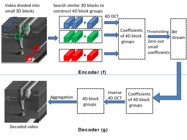
Figure 4: Encoder (upper part) and decoder (lower part) by exploiting the nonlocal similarity of videos.

The encoding operation includes performing the following steps:

• Divide the 3D video ${\bf X}\in{\mathbb{R}}^{n_{x}\times n_{y}\times B}$ into small overlapping blocks ${\cal X}_{q}\in{\mathbb{R}}^{p_{x}\times p_{y}\times B}$, $q=1,\dots,Q$, where $Q$ denotes the number of such small 3D blocks.

• For each reference block, ${\cal X}_{q}$, find its “similar” blocks between the remaining $Q-1$ blocks. The similarity between two blocks is measured in terms of their $\ell_{2}$-norm distance. For ${\cal X}_{q}$, the encoder picks its $G$ most similar blocks, thus forms a 4-way tensor $\tilde{\cal X}_{q}\in{\mathbb{R}}^{p_{x}\times p_{y}\times B\times G}$. These similar blocks are sorted based on their $\ell_{2}$-norm distances, from the smallest to the largest and thus the reference block is always the first one.

• Apply 4D DCT (discrete Cosine transformation) to each 4D block group, and derive the 4D coefficients for each block group. For each group of blocks, since the blocks are very similar, the coefficients will be sparse in the transform domain.

• Set the coefficients with small amplitudes to zero. More specifically, the encoder only keeps $p_{x}p_{y}B$ (out of $p_{x}p_{y}bG$) coefficients with largest amplitudes for each block group. In total, there will be $p_{x}p_{y}BQ$ non-zero coefficients for the entire video since there are $Q$ 3D blocks.

• Encode the remaining $p_{x}p_{y}BQ$ non-zero coefficients and their corresponding locations and their group indices.

Note that there are significant redundancies in this encoder since each pixel has been encoded many times, which will help the decoder to achieve videos with higher quality.

Correspondingly, the decoder includes the following steps.

• Decode the non-zero coefficients and their corresponding locations and group indices.

• Fill in the zero coefficients to get the coefficients of 4D block groups.

• Perform inverse 4D DCT to the coefficients of each 4D block group.

• Put the blocks back to the original locations and aggregate these blocks (taking average value of each pixel) to achieve the decoded video.

References

- [1] S. Jalali and X. Yuan, “Compressive imaging via one-shot measurements,” in IEEE International Symposium on Information Theory (ISIT), 2018.
- [2] E. Candès, J. Romberg, , and T. Tao, “Robust uncertainty principles: Exact signal reconstruction from highly incomplete frequency information,” IEEE Trans. Inform. Theory, vol. 52, no. 2, pp. 489–509, Feb. 2006.
- [3] D. L. Donoho, “Compressed sensing,” IEEE Trans. Inform. Theory, vol. 52, no. 4, pp. 1289–1306, April 2006.
- [4] M. F. Duarte, M. A. Davenport, D. Takhar, J. N. Laska, T. Sun, K. F. Kelly, and R. G. Baraniuk, “Single-pixel imaging via compressive sampling,” IEEE Sig. Proc. Mag., vol. 25, no. 2, pp. 83–91, 2008.
- [5] L. Gao, J. J. Liang, C. Li, and L. V. Wang, “Single-shot compressed ultrafast photography at one hundred billion frames per second,” Nature, vol. 516, pp. 49–57, 2014.
- [6] M. E. Gehm, R. John, D. J. Brady, R. M. Willett, and T. J. Schulz, “Single-shot compressive spectral imaging with a dual-disperser architecture,” Optics Exp., vol. 15, pp. 14 013–14 027, 2007.
- [7] Y. Hitomi, J. Gu, M. Gupta, T. Mitsunaga, and S. K. Nayar, “Video from a single coded exposure photograph using a learned over-complete dictionary,” in IEEE Int. Conf. on Comp. Vis. (ICCV), 2011.
- [8] P. Llull, X. Liao, X. Yuan, J. Yang, D. Kittle, L. Carin, G. Sapiro, and D. J. Brady, “Coded aperture compressive temporal imaging,” Optics Exp., vol. 21, no. 9, pp. 10 526–10 545, May 2013.
- [9] D. Reddy, A. Veeraraghavan, and R. Chellappa, “P2C2: Programmable pixel compressive camera for high speed imaging,” IEEE Comp. Vis. and Pat. Rec. (CVPR), 2011.
- [10] A. Wagadarikar, R. John, R. Willett, and D. J. Brady, “Single disperser design for coded aperture snapshot spectral imaging,” App. Optics, vol. 47, no. 10, pp. B44–B51, 2008.
- [11] A. Wagadarikar, N. Pitsianis, X. Sun, and D. Brady, “Video rate spectral imaging using a coded aperture snapshot spectral imager,” Opt. Express, vol. 17, no. 8, pp. 6368–6388, Apr. 2009.
- [12] G. Huang, H. Jiang, K. Matthews, and P. Wilford, “Lensless imaging by compressive sensing,” IEEE Int. Conf. on Image Proc., 2013.
- [13] A. C. Sankaranarayanan, L. Xu, C. Studer, Y. Li, K. F. Kelly, and R. G. Baraniuk, “Video compressive sensing for spatial multiplexing cameras using motion-flow models,” SIAM J. on Imag. Sci., vol. 8, no. 3, pp. 1489–1518, 2015.
- [14] W. U. Bajwa, J. D. Haupt, G. M. Raz, S. J. Wright, and R. D. Nowak, “Toeplitz-structured compressed sensing matrices,” in 2007 IEEE/SP 14th Workshop on Statistical Sig. Proc., Aug 2007, pp. 294–298.
- [15] J. Romberg, “Compressive sensing by random convolution,” SIAM J. on Imaging Sciences, vol. 2, no. 4, pp. 1098–1128, 2009.
- [16] E. J. Candes and Y. Plan, “A probabilistic and ripless theory of compressed sensing,” IEEE Trans. Inform. Theory, vol. 57, no. 11, pp. 7235–7254, 2011.
- [17] A. Eftekhari, H. L. Yap, C. J. Rozell, and M. B. Wakin, “The restricted isometry property for random block diagonal matrices,” Appl. Comp. Harmonic Anal. (ACHA), vol. 38, no. 1, pp. 1–31, 2015.
- [18] S. Foucart and H. Rauhut, “A mathematical introduction to compressive sensing,” Bull. Am. Math, vol. 54, pp. 151–165, 2017.
- [19] B. Adcock, A. C. Hansen, C. Poon, and B. Roman, “Breaking the coherence barrier: A new theory for compressed sensing,” in Forum of Math., Sigma, vol. 5. Cambridge University Press, 2017.
- [20] C. Boyer, J. Bigot, and P. Weiss, “Compressed sensing with structured sparsity and structured acquisition,” Appl. Comp. Harmonic Anal. (ACHA), 2017.
- [21] P. Llull, X. Yuan, L. Carin, and D. Brady, “Image translation for single-shot focal tomography,” Optica, vol. 2, no. 9, pp. 822–825, 2015.
- [22] X. Yuan, P. Llull, X. Liao, J. Yang, G. Sapiro, D. J. Brady, and L. Carin, “Low-cost compressive sensing for color video and depth,” in IEEE Conf. on Com. Vis. and Pat. Rec. (CVPR), 2014.
- [23] T.-H. Tsai, X. Yuan, and D. J. Brady, “Spatial light modulator based color polarization imaging,” Optics Express, vol. 23, no. 9, pp. 11 912–11 926, May 2015.
- [24] T.-H. Tsai, P. Llull, X. Yuan, D. J. Brady, and L. Carin, “Spectral-temporal compressive imaging,” Optics Letters, vol. 40, no. 17, pp. 4054–4057, Sep. 2015.
- [25] S. Jalali and A. Maleki, “From compression to compressed sensing,” Appl. Comp. Harmonic Anal. (ACHA), vol. 40, no. 2, pp. 352–385, 2016.
- [26] J. Yang, X. Yuan, X. Liao, P. Llull, G. Sapiro, D. J. Brady, and L. Carin, “Video compressive sensing using Gaussian mixture models,” IEEE Trans. on Image Proc., vol. 23, no. 11, pp. 4863–4878, Nov. 2014.
- [27] J. Yang, X. Liao, X. Yuan, P. Llull, D. J. Brady, G. Sapiro, and L. Carin, “Compressive sensing by learning a Gaussian mixture model from measurements,” IEEE Trans. on Image Proc., vol. 24, no. 1, pp. 106–119, Jan. 2015.
- [28] X. Yuan, T.-H. Tsai, R. Zhu, P. Llull, D. J. Brady, and L. Carin, “Compressive hyperspectral imaging with side information,” IEEE J. of Sel. Topics in Sig. Proc., vol. 9, no. 6, pp. 964–976, Sep. 2015.
- [29] E. Candes and J. Romberg, “Sparsity and incoherence in compressive sampling,” Inv. Prob., vol. 23, no. 3, pp. 969–985, 2007.
- [30] J. Huang, T. Zhang, and D. Metaxas, “Learning with structured sparsity,” in Proceedings of the 26th Annual International Conference on Machine Learning, ser. ICML ’09, 2009, pp. 417–424.
- [31] R. G. Baraniuk, V. Cevher, M. F. Duarte, and C. Hegde, “Model-based compressive sensing,” IEEE Trans. Inform. Theory, vol. 56, no. 4, pp. 1982–2001, April 2010.
- [32] W. Dong, G. Shi, X. Li, Y. Ma, and F. Huang, “Compressive sensing via nonlocal low-rank regularization,” IEEE Trans. on Image Proc., vol. 23, no. 8, pp. 3618–3632, 2014.
- [33] C. A. Metzler, A. Maleki, and R. G. Baraniuk, “From denoising to compressed sensing,” IEEE Trans. Inform. Theory, vol. 62, no. 9, pp. 5117–5144, Sep. 2016.
- [34] D. S. Taubman and M. W. Marcellin, JPEG2000: Image Compression Fundamentals, Standards and Practice. Kluwer Academic Publishers, 2002.
- [35] S. Beygi, S. Jalali, A. Maleki, and U. Mitra, “An efficient algorithm for compression-based compressed sensing,” A Journal of IMA: Inform. and Inf., 2018.
- [36] J. Holloway, A. C. Sankaranarayanan, A. Veeraraghavan, and S. Tambe, “Flutter shutter video camera for compressive sensing of videos,” in 2012 IEEE Int. Conf. on Comp. Phot. (ICCP), April 2012, pp. 1–9.
- [37] H. Arguello, H. Rueda, Y. Wu, D. W. Prather, and G. R. Arce, “Higher-order computational model for coded aperture spectral imaging,” Appl. Opt., vol. 52, no. 10, pp. D12–D21, Apr 2013.
- [38] R. G. Baraniuk, T. Goldstein, A. C. Sankaranarayanan, C. Studer, A. Veeraraghavan, and M. B. Wakin, “Compressive video sensing: Algorithms, architectures, and applications,” IEEE Sig. Proc. Magazine, vol. 34, no. 1, pp. 52–66, Jan 2017.
- [39] G. R. Arce, D. J. Brady, L. Carin, H. Arguello, and D. S. Kittle, “Compressive coded aperture spectral imaging: An introduction,” IEEE Sig. Proc. Magazine, vol. 31, no. 1, pp. 105–115, Jan 2014.
- [40] X. Cao, T. Yue, X. Lin, S. Lin, X. Yuan, Q. Dai, L. Carin, and D. J. Brady, “Computational snapshot multispectral cameras: Toward dynamic capture of the spectral world,” IEEE Sig. Proc. Magazine, vol. 33, no. 5, pp. 95–108, Sept 2016.
- [41] Y. Nesterov, Introductory lectures on convex optimization: A basic course. Springer Science & Business Media, 2013, vol. 87.
- [42] H. Attouch, J. Bolte, and B. F. Svaiter, “Convergence of descent methods for semi-algebraic and tame problems: proximal algorithms, forward–backward splitting, and regularized gauss–seidel methods,” Math. Prog., vol. 137, no. 1-2, pp. 91–129, 2013.
- [43] X. Liao, H. Li, and L. Carin, “Generalized alternating projection for weighted- minimization with applications to model-based compressive sensing,” SIAM J. on I,ag. Sci., vol. 7, no. 2, pp. 797–823, 2014.
- [44] X. Yuan, “Adaptive step-size iterative algorithm for sparse signal recovery,” Sig. Proc., vol. 152, pp. 273–285, 2018.
- [45] M. Iliadis, L. Spinoulas, and A. K. Katsaggelos, “Deep fully-connected networks for video compressive sensing,” Digital Sig. Proc., vol. 72, pp. 9 – 18, 2018.
- [46] K. Xu and F. Ren, “CSVideoNet: A real-time end-to-end learning framework for high-frame-rate video compressive sensing,” ArXiv e-prints, Dec. 2016.
- [47] X. Yuan, “Generalized alternating projection based total variation minimization for compressive sensing,” in IEEE Int. Conf. on Image Proc. (ICIP), Sep. 2016, pp. 2539–2543.
- [48] D. Le Gall, “MPEG: A video compression standard for multimedia applications,” Communications of the ACM, vol. 34, no. 4, pp. 46–58, Apr. 1991.
- [49] J. A. Nelder and R. Mead, “A simplex method for function minimization,” Computer Journal, vol. 7, pp. 308–313, 1965.
- [50] A. Buades, B. Coll, and J.-M. Morel, “A non-local algorithm for image denoising,” in Proceedings of the 2005 IEEE Computer Society Conference on Computer Vision and Pattern Recognition (CVPR’05) - Volume 2 - Volume 02, ser. CVPR ’05, 2005, pp. 60–65.
- [51] K. Dabov, A. Foi, V. Katkovnik, and K. Egiazarian, “Image denoising by sparse 3d transform-domain collaborative filtering,” IEEE Trans. on Image Proc., vol. 16, no. 8, pp. 2080–2095, August 2007.
- [52] M. Maggioni, G. Boracchi, A. Foi, and K. Egiazarian, “Video denoising, deblocking, and enhancement through separable 4-d nonlocal spatiotemporal transforms,” IEEE Trans. on Image Processing, vol. 21, no. 9, pp. 3952–3966, Sept 2012.
- [53] Y. Liu, X. Yuan, J. Suo, D. Brady, and Q. Dai, “Rank minimization for snapshot compressive imaging,” IEEE Trans. on Pattern Analysis and Machine Intelligence, pp. 1–1, 2018.
- [54] W. Dong, L. Zhang, G. Shi, and X. Li, “Nonlocally centralized sparse representation for image restoration,” IEEE Trans. on Image Processing, vol. 22, no. 4, pp. 1620–1630, April 2013.
- [55] H. Liu, R. Xiong, J. Zhang, and W. Gao, “Image denoising via adaptive soft-thresholding based on non-local samples,” in 2015 IEEE Conference on Computer Vision and Pattern Recognition (CVPR), June 2015, pp. 484–492.
- [56] “Runner data,” https://www.videvo.net/video/elite-runner-slow-motion/4541/.
- [57] R. Vershynin, “Introduction to the non-asymptotic analysis of random matrices,” arXiv preprint arXiv:1011.3027, 2010.
- [58] Y. Sun, X. Yuan, and S. Pang, “High-speed compressive range imaging based on active illumination,” Optics Express, vol. 24, no. 20, pp. 22 836–22 846, Oct 2016.
- [59] ——, “Compressive high-speed stereo imaging,” Optics Express, vol. 25, no. 15, pp. 18 182–18 190, July 2017.
- [60] D. Huang, E. Swanson, C. Lin, J. Schuman, W. Stinson, W. Chang, M. Hee, T. Flotte, K. Gregory, C. Puliafito, and a. et, “Optical coherence tomography,” Science, vol. 254, no. 5035, pp. 1178–1181, 1991.
- [61] A. Kirmani, D. Venkatraman, D. Shin, A. Colaço, F. N. C. Wong, J. H. Shapiro, and V. K. Goyal, “First-photon imaging,” Science, vol. 343, no. 6166, pp. 58–61, 2014.