Natural Groundwater Systems Can Display Chaotic Mixing at the Darcy Scale

Abstract

Although steady, isotropic Darcy flows are inherently laminar and non-mixing, it is well understood that transient forcing via engineered pumping schemes can induce rapid, chaotic mixing in groundwater. In this study we explore the propensity for such mixing to arise in natural groundwater systems subject to cyclical forcings, e.g. tidal or seasonal influences. Using a conventional linear groundwater flow model subject to tidal forcing, we show that under certain conditions these flows generate Lagrangian transport and mixing phenomena (chaotic advection) near the tidal boundary. We show that aquifer heterogeneity, storativity, and forcing magnitude cause reversals in flow direction over the forcing cycle which, in turn, generate coherent Lagrangian structures and chaos. These features significantly augment fluid mixing and transport, leading to anomalous residence time distributions, flow segregation, and the potential for profoundly altered reaction kinetics. We define the dimensionless parameter groups which govern this phenomenon and explore these groups in connection with a set of well-characterised coastal systems. The potential for Lagrangian chaos to be present near discharge boundaries must be recognized and assessed in field studies.

Key Points:

• Time-periodic Darcy flows in heterogeneous compressible aquifers can generate chaotic mixing dynamics

• Widespread occurrence of coherent Lagrangian structures is controlled by key parameter groups and results from common physical processes

• Such structures fundamentally change our view of flow, transport, mixing and reaction in groundwater discharge systems

1 Introduction

For well over a century it has been known that steady isotropic Darcy flows are inherently poor mixing flows. Seminal works by Kelvin (1884) and Arnol’d (1965) established that the streamlines of these flows are confined to two-dimensional (2D) lamellar sheets (thus termed “complex lamellar” flows), which significantly restricts their transport behaviour. This kinematic constraint is a direct consequence of the helicity-free nature of Darcy flow, in that the helicity density of these flows (defined as the dot product of vorticity and velocity (Moffatt, 1969)), which characterises helical twisting of streamlines, is identically zero, confining streamlines to coherent lamellar sheets. Confinement restricts stretching of fluid elements to be at most algebraic in time (Dentz et al., 2016), limiting growth of material interfaces and hence mixing. Steady isotropic Darcy flows may be strongly heterogeneous, but they exhibit slow (algebraic) deformation of fluid elements and poor mixing.

Conversely, transient isotropic Darcy flows break this kinematic constraint as the confining lamellae can change with time, leading to the possibility of chaotic mixing which is characterised by exponential stretching of fluid elements (Ottino, 1989). Over the last decade it has been established that such rapid mixing may be engineered at the Darcy scale (metres to kilometres) in groundwater systems through the use of programmed pumping activities (Sposito, 2006; Bagtzoglou and Oates, 2007; Metcalfe et al., 2007; Lester et al., 2009, 2010; Metcalfe et al., 2010b, a, 2011; Trefry et al., 2012; Mays and Neupauer, 2012; Piscopo et al., 2013; Rodríguez-Escales et al., 2017; Cho et al., 2017), with selectable and comprehensive consequences for contaminant migration and fate. The saturated zone may now be regarded as a reaction vessel whose mixing state may be manipulated in order to promote reactivity or segregation according to the requirements of groundwater quality management. This is a significant paradigm shift for groundwater systems which have long been thought to be governed by poor mixing and transport characteristics unamenable to external control.

Now that we can engineer chaotic mixing in groundwater systems, we may consider the supplementary question, is chaotic mixing a natural characteristic of groundwater systems? If so, the ramifications for flow, transport and reaction in groundwater systems are likely to be as profound as those demonstrated elsewhere for chaotic flows in diverse areas of science (see e.g. Tél et al. (2005) or Aref et al. (2017)). In order to answer this question we seek natural (unmodified by human intervention) and common aquifer settings that engender the basic preconditions for Lagrangian chaos, namely repeated stretching and folding of fluid elements, widely considered a hallmark of chaotic advection (Ottino, 1989). If we can demonstrate that such conditions occur in natural settings, and we can quantify how these lead to chaotic mixing, then we will have established that such kinematics are a natural phenomenon in a broad class of groundwater systems. This demonstration is the purpose of this paper.

This question has been partially answered in the context of steady anisotropic Darcy flows, which do not conform to the kinematic constraints of isotropic Darcy flow (they are not helicity-free) and have been shown both numerically (Cirpka et al., 2012) and experimentally (Ye et al., 2015) to exhibit the accelerated mixing dynamics characteristic of chaotic mixing. In this study we determine to what extent transient forcings can generate chaotic mixing in natural groundwater systems. Many natural groundwater systems are driven by discharge boundaries at rivers, lakes and coasts, which are always time-dependent to some degree through tidal action, seasonal, and barometric effects etc. In principle, transient forcings are sufficient to break the zero helicity kinematic constraint, but to generate chaotic mixing at the Darcy scale these must also lead to stretching and folding fluid motions: changes in flow orientation and reorganisation of the flow streamlines are necessary to achieve persistent stretching and folding of material elements. As such, natural groundwater systems near discharge boundaries represent likely candidates for chaotic mixing because the interaction between transient forcing at the discharge boundary combined with spatial heterogeneity of aquifer properties (intrinsic to all groundwater systems) provides a mechanism for strong flow reorientation over the forcing cycle. Indeed, these physical phenomena influence the transport and fate of groundwater contaminants at the intertidal zones, leading to complex spatio-temporal distributions of biogeochemical reactivity (Heiss et al., 2017; Liu et al., 2017; Malott et al., 2017; Kobayashi et al., 2017). Fluid mixing, dilution and residence time have been correlated with enhanced biodegradation rates for contaminants in coastal aquifers subject to tidal influences (Robinson et al., 2009; Geng et al., 2017). Since chaotic mixing can fundamentally alter reaction kinetics, leading to e.g. singularly enhanced reaction rates (Toroczkai et al., 1998), we hypothesize that chaotic processes may contribute to groundwater discharge and reaction complexity in coastal zones. Accordingly, for the remainder of this paper we focus on coastal aquifers as likely candidates for natural chaotic mixing.

In pursuing this approach we seek to reduce the complexity of the physical model in order to emphasize the source and nature of key chaotic processes. Thus, we are concerned with confined, isohaline systems (zero density differences) in two dimensions (plan view), resulting in a linear flow equation within a simple rectangular domain. Issues of capillarity and beach slope are ignored in this study, as are solute transport and dispersion. These assumptions are contrary to established theoretical approaches for studying groundwater discharge and reaction in coastal systems; however, our contention is that if conditions are right for chaotic signatures to occur in our simple model tidal flow system, then such signatures are also possible in more realistic models conditioned on field observations.

We proceed as follows. After a brief survey of chaotic fluid processes in porous media, the paper introduces a conventional model 2D Darcian system representing a heterogeneous, tidally forced confined aquifer that is used as a basis for a Lagrangian analysis of the flow regime. The tidal flow problem is solved numerically and the basic solution properties are explored, focusing on the flux and velocity distributions. In subsequent sections key dimensionless parameter groups are introduced to assist in predicting the onset of chaotic mixing, a survey of Lagrangian and chaotic phenomena arising in the model tidal system is presented, and comments are made on the potential ramifications for biogeochemical processes acting at tidal discharge boundaries.

2 Chaotic advection in porous media flows

At the pore scale, fluid advection and mixing within the pore space $\Omega$ is governed by the Stokes equation (1) subject to no-slip conditions at the fluid boundary $\partial\Omega$

$$\mu\nabla^{2}\mathbf{v}(\mathbf{x})-\nabla p(\mathbf{x})=\mathbf{0},\quad\nabla\cdot\mathbf{v}(\mathbf{x})=0,\quad\mathbf{x}\in\Omega,\quad\mathbf{v}(\mathbf{x})\big{|}_{\mathbf{x}\in\partial\Omega}=0,$$ (1)

where $\mu$ is the dynamic viscosity, $p$ is the fluid pressure, $\nabla^{2}$ is the vector Laplacian operator, and $\mathbf{v}$ is the fluid velocity vector of the pure fluid within the pore space $\Omega$. This boundary-dominated flow is controlled by the geometry and connectivity of the pore space. Three-dimensional steady Stokes flows engender chaotic mixing due to the topological complexity inherent to all porous media (Lester et al., 2013a, 2016a), and the resulting pore-scale transport signatures persist into the macroscale (Lester et al., 2016b, 2014a).

Whilst these models provide insights into dispersion and mixing at the pore scale, continuum flow models that utilise averaged microscale pore and fluid properties are more widely used. These models are employed in the analysis of macroscale systems for which observational data are often scarce and the difficulties of microscale system characterisation and upscaling are usually insurmountable. In the groundwater domain, the Darcy flow equation (Darcy, 1856; Whitaker, 1986) is a useful continuum model, relating fluid flux through a porous medium to imposed pressure gradient. Despite the ubiquity of pore-scale chaotic mixing, Darcy flows are laminar and poorly mixing due to the zero helicity kinematic constraint. It was not recognised until recently (Sposito, 2006; Bagtzoglou and Oates, 2007; Metcalfe et al., 2007; Lester et al., 2009; Metcalfe et al., 2010a; Trefry et al., 2012; Piscopo et al., 2013) that Darcian systems could display chaotic signatures which underpin mixing enhancement which may be beneficial for contaminant remediation (Rodríguez-Escales et al., 2017). The mechanism generating macroscale chaotic mixing is the “crossing” of streamlines (when viewed at different times) which can lead to stretching and folding of the flow. Repeated changes of fluid flow direction can enhance reaction in porous media (Zhang et al., 2009) and, critically, produce kinematic effects (Trefry et al., 2012) ranging from the creation of kinematic transport “barriers” to rapid, global mixing. A key hydrogeological example is the programmed rotated potential mixing (RPM) flow (Lester et al., 2009; Metcalfe et al., 2010b) which can be generated in the field by sets of injection/extraction wells operating under a synchronised dipole pumping schedule (Cho et al., 2017). Three-dimensional variants of the RPM flow have also been studied (Smith et al., 2016; Cho et al., 2017), showing controllable 3D chaotic mixing is possible in porous media flows at the Darcy scale.

For natural Darcy flows we need a quantitative, computable metric that definitively indicates whether chaos exists in the flow or not. The Lyapunov exponent is commonly used in dynamical systems to measure the sensitivity of a system to its initial conditions; it directly characterises the rate of exponential growth of (infinitesimal) material elements (see for example Allshouse and Peacock, 2015) in both volume-preserving flows and more recently, non-volume-preserving flows (Volk et al., 2014; González et al., 2016; Pérez-Muñuzuri, 2014). The time-dependent groundwater equation (5) describes a non-volume-preserving flow due to the storage term, and typically corresponds to an open flow (Tél et al., 2005) due to the in- and outflow boundaries typical of hydrogeological models. In this study we use the presence of a positive Lyapunov exponent (indicating the presence of exponential fluid stretching) as an indicator of chaotic mixing. We now turn to a formal problem definition for our tidally forced system.

3 Transient flow in tidally forced aquifers

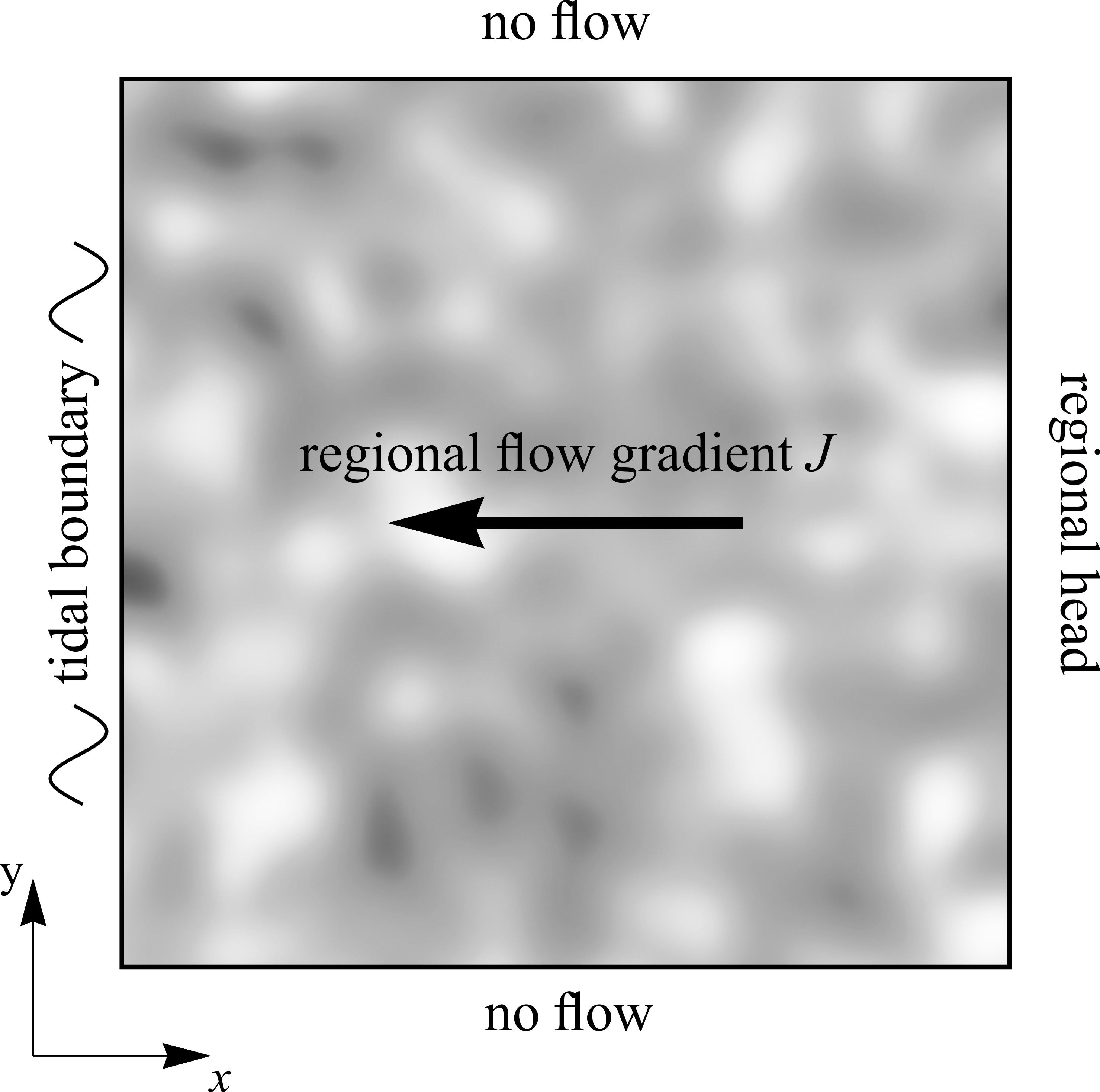
Figure 1: Schematic of the square aquifer domain $\mathcal{D}$ and boundaries, showing the regional flow gradient $J$ and spatial heterogeneity of $K$.

As a prototype of a coastal aquifer, we consider a bounded 2D domain in the $x-y$ plane representing an aquifer in plan view, that is the aquifer domain $\mathcal{D}$ is defined by the coordinate $\textbf{x}=(x,y)\in[0,L_{x}]\times[0,L_{y}]$. We assume the aquifer has unit thickness $B=1$. For numerical simplicity and without loss of generality we assume $L_{x}=L_{y}=L$, as depicted in Figure 1. Furthermore we limit our analysis to confined flow conditions in the absence of vertical recharge and internal sources and sinks. Following Bear (1972) we write the continuity equation for an incompressible fluid in a deformable porous medium of matrix porosity $\varphi$ as

$$\dfrac{\partial\varphi}{\partial t}+\nabla\cdot\mathbf{q}=0,$$ (2)

where the Darcy flux $\mathbf{q}=\varphi\mathbf{v}$ (with $\mathbf{v}$ the groundwater velocity) is given by the Darcy equation

$$\textbf{q}=-K\nabla h,$$ (3)

where the spatially heterogeneous scalar $K(\mathbf{x})$ is the isotropic saturated hydraulic conductivity and $h$ is the pressure head. For 2D systems it is usual to work in terms of the transmissivity $T=KB$; however, as $B=1$ we use $K$ throughout. Following conventional approaches (Bear, 1972; Coussy, 2004), we model changes in the local porosity $\varphi$ due to fluctuations in the local head $h$ via a linear approximation

$$\varphi(h)=\varphi_{\textrm{ref}}+S\!_{s}\;(h-h_{\textrm{ref}}),$$ (4)

where $h_{\textrm{ref}}$ is the reference head at which the reference porosity $\varphi_{\textrm{ref}}$ applies, and $S\!_{s}$ is formally the specific storage. However, noting the unit aquifer thickness assumption we henceforth replace $S\!_{s}$ by $S$ and refer to the storage term simply as storativity. As $\varphi_{\textrm{ref}}$, $h_{\textrm{ref}}$ and $S$ are assumed constant, all spatial and temporal dependence of $\varphi$ is generated by the coupling with $h$. It is important to note that whilst the solid phase in most aquifers is essentially incompressible, equation (4) models changes in local porosity with head as an effective compressibility. This conventional approximation avoids the complication of explicitly solving the solids phase displacement (Bear, 1972), but does not fully capture the migration of solids in the aquifer due to pressure gradients. Combining (2)-(4) yields the linear groundwater flow equation

$$S\dfrac{\partial h}{\partial t}=\nabla\cdot(K\nabla h),$$ (5)

subject to the no flow, inland fixed head ($J$ the inland head gradient) and tidal boundary conditions ($g(t)$), respectively,

$$\dfrac{\partial h}{\partial y}\Bigr{|}_{y=0}=\dfrac{\partial h}{\partial y}\Bigr{|}_{y=L}=0, h(L,y,t)=JL, h(0,y,t)=\textsl{g}(t).$$ (6)

Solution of the groundwater equation (5) subject to the boundary conditions (6) completely solves the system, and the Darcy flux $\mathbf{q}$ is computed via (3). The inland boundary condition $JL$ is intended to provide for mean discharge flow to the tidal boundary, i.e. $JL>\overline{\textsl{g}(t)}$, which is common in the field. Nevertheless, saline intrusion $JL<\overline{\textsl{g}(t)}$ is becoming more widespread (see, e.g. Fadili et al., 2018). Our model encompasses mean intrusion from the tidal boundary, but in this work we restrict attention solely to discharging regional flows.

3.1 Steady and periodic solutions

Following Trefry et al. (2011), we assume the tidal boundary forcing function $\textsl{g}(t)$ to be finite-valued and cyclic with period $P$, i.e. $\textsl{g}(t)=\textsl{g}(t+P)$. For simplicity of exposition we assume the tidal forcing to consist of a single Fourier mode

$$\textsl{g}(t)=\textsl{g}_{p}e^{i\omega t},$$ (7)

where $\omega$ is the forcing frequency, and note that extension to a multi-modal tidal forcing spectrum does not alter qualitative aspects of the problem (Trefry and Bekele, 2004). Under such forcing, the head $h$ can be decomposed into steady $h_{s}$ and periodic $h_{p}$ components

$$h(\textbf{x},t)=h_{s}(\textbf{x})+h_{p}(\textbf{x},t)=h_{s}(\textbf{x})+h_{p,x}(\textbf{x})e^{i\omega t}$$ (8)

that satisfy the steady and periodic Darcy equations, respectively,

$$\nabla\cdot(K\nabla h_{s}(\mathbf{x}))=0, \nabla\cdot(K\nabla h_{p,x}(\mathbf{x}))-i\omega Sh_{p,x}(\mathbf{x})=0,$$ (9)

subject to the boundary conditions

$$h_{s}(L,y)=JL, h_{s}(0,y)=0, h_{p,x}(L,y)=0, h_{p,x}(0,y) =\textsl{g}_{p}$$ (10)

with zero flux conditions for both $h_{s}$, $h_{p,x}$ at the $y=0$ and $y=L$ boundaries. All periodic quantities are complex in this formulation, and so the real part must be taken throughout as these are observable quantities. Henceforth we drop the notations $h_{p,x}$ for the spatial part of the periodic head component, replacing it by $h_{p}$. It is understood that formally $h_{p}(\mathbf{x},t)\equiv h_{p}(\mathbf{x})e^{i\omega t}$. Likewise, the porosity relation (4) can be decomposed into steady and periodic contributions as

$$\varphi(\mathbf{x},t)=\varphi_{s}(\mathbf{x})+\varphi_{p}(\mathbf{x},t)=\varphi_{\textrm{ref}}+S(h_{s}(\mathbf{x})-h_{\textrm{ref}})+Sh_{p}(\mathbf{x},t),$$ (11)

where $\varphi_{p}$ is the last term on the right hand side of (11).

3.2 Hydraulic characteristics

Early analytical results for tidal influences in one-dimensional aquifers with uniform and homogeneous $K$ fields were derived for semi-infinite domains by Jacob (1950) and were extended to finite (Townley, 1995), layered (Li and Jiao, 2002) and composite (Trefry, 1999) domains. Analytical results were also obtained in two dimensions for uniform (Li et al., 2000) and stochastic (Trefry et al., 2011) aquifer property distributions. Many other analytical results for tidal groundwater systems have been reported.

A key feature of the tidal solutions is a finite propagation speed from the tidal boundary to the interior, so that induced oscillations measured at locations inside the aquifer domain are lagged (out of phase) and attenuated (reduced in amplitude) with respect to the boundary forcing condition. For a one-dimensional, semi-infinite homogeneous aquifer, the phase lag $\Delta\tau$ and attenuation $\alpha$ are related to the forcing frequency $\omega$, aquifer diffusivity $D=K/S$ and distance $x$ from the tidal boundary as (Jacob, 1950; Ferris, 1951)

$$\Delta\tau=x/\sqrt{2\omega D}, \alpha=\textrm{exp}\left(-x\sqrt{\omega/2D}\right).$$ (12)

The dissipative nature of the periodic equation (9) provides an exponential decay of oscillation amplitude with distance from the forcing boundary and phase lag increasing linearly with distance, with the attenuation greatest for high $\omega$ and least for low $\omega$. The Electronic Supplementary Material accompanying this paper contains example animations of the solution head distribution, velocity ellipses (Section 3.3) and the vorticity (Appendix B). The animations show the finite propagation speed of head disturbances in the aquifer domain and the effect of $K$ heterogeneity.

3.3 Flux ellipses and flow reversal

As shown by Kacimov et al. (1999) and Smith et al. (2005), time-periodic groundwater forcing causes elliptical velocity orbits at each point in the aquifer domain. More precisely, the family of possible velocity orbits includes ellipses, circles, lines and points, depending on degeneracies in the semi-axes and component phases of the underlying flux ellipses. Returning to the present tidal problem, the induced Darcy flux $\mathbf{q}(\mathbf{x},t)=(q_{x},q_{y})$ at a location $\textbf{x}=(x,y)$ and time $t$ can also be decomposed into steady and periodic components as

$$\mathbf{q}(\mathbf{x},t)=\mathbf{q}_{s}(\mathbf{x})+\mathbf{q}_{p}(\mathbf{x},t)\equiv\mathbf{q}_{s}(\mathbf{x})+\mathbf{q}_{p}(\mathbf{x})e^{i\omega t},$$ (13)

where $\mathbf{q}_{s}=-K\nabla h_{s}$, $\mathbf{q}_{p}=-K\nabla h_{p}$. For any location $\mathbf{x}$ in the flow domain, the steady flux $\mathbf{q}_{s}(\mathbf{x})$ fixes the location of the flux ellipse shown in in Figure 2, whereas the periodic flux $\mathbf{q}_{p}(\mathbf{x},t)$ governs the orientation, eccentricity and magnitude of the modal flux ellipse that is swept out parametrically with $t$ over a flow period. The sign of $\mathbf{q}_{p}$ dictates whether the flux ellipse is traced out clockwise or anti-clockwise in time. For more complex multi-modal tidal forcing $\textsl{g}(t)$, the orbit traced out by $\mathbf{q}$ may be more complex than a simple ellipse but the qualitative aspects of the system are conserved.

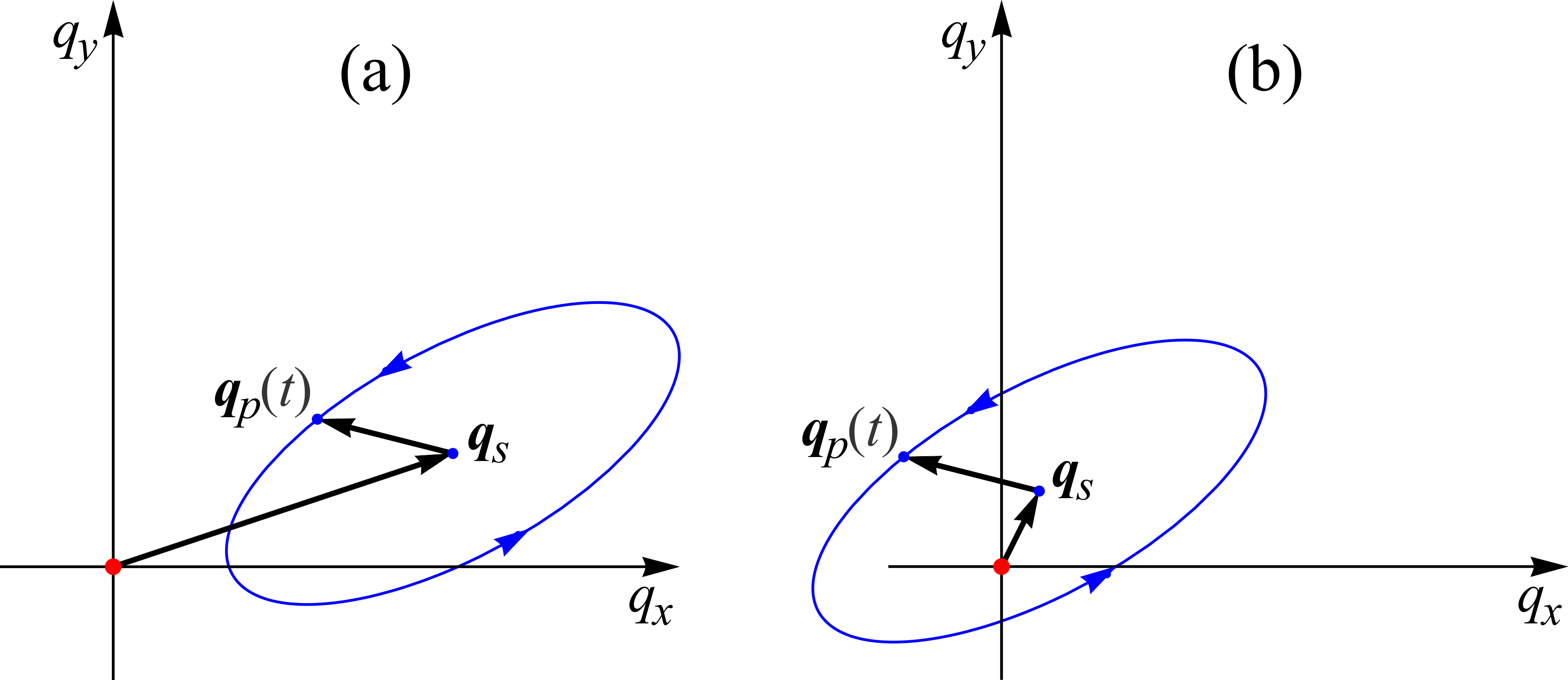
Figure 2: Schematic of flux ellipses drawn in blue - (a) regular (excluding the origin), and (b) canonical (containing the origin). Arrows on the ellipses indicate the direction of increasing time $t$. Both flux components of the canonical ellipse change sign at times during the oscillation period.

Under the condition that the magnitude of the periodic flux is greater than that of the steady flux at a given point $\mathbf{x}$, i.e. $||\mathbf{q}_{p}(\mathbf{x})||>||\mathbf{q}_{s}(\mathbf{x})||$, then flow reversal occurs at some time in the flow cycle, i.e. the total flux $\mathbf{q}$ is in the opposite direction to the steady flux $\mathbf{q}_{s}$, and the flux ellipse over the entire flow cycle contains the origin $\mathbf{q}=\mathbf{0}$. Flux ellipses that contain the origin (and hence admit flow reversal) will henceforth be referred to as canonical. In Appendix B we show that flow reversal occurs due to the interplay between conductivity variations and compressibility of the aquifer.

As shown in Appendix D, for incompressible aquifers ($S=0$) the periodic flux vector $\mathbf{q}_{p}(\mathbf{x},t)$ aligns with the steady flux vector $\mathbf{q}_{s}(\mathbf{x})$ and the sign and magnitude of $\mathbf{q}_{p}$ simply oscillates over a tidal forcing cycle. Consequently the flux ellipses in the incompressible limit have zero width (or infinite eccentricity). This leads to fluid particle trajectories that follow simple, smooth streamlines (although particles move backwards and forwards as they propagate along these streamlines), leading to regular, non-chaotic fluid motion. Accordingly, we denote any flux ellipse with an eccentricity greater than 100 as a trivial ellipse as it will not contribute significantly to complex fluid motion.

3.4 Fluid velocity and Lagrangian kinematics

As fluid particles and passive tracers are advected by the groundwater velocity $\mathbf{v}=\mathbf{q}/\varphi$, in this study we are primarily interested in the mixing and transport properties of $\mathbf{v}(\mathbf{x},t)$. For finite $S>0$, $\varphi$ varies with space and time through its dependence on $h$, and it is not possible to separate v into steady and periodic terms; rather, $\mathbf{v}$ is given by

$$\mathbf{v}(\mathbf{x},t)=\dfrac{\mathbf{q}(\mathbf{x},t)}{\varphi(\mathbf{x},t)}=\dfrac{\mathbf{q}_{s}(\mathbf{x})+\mathbf{q}_{p}(\mathbf{x},t)}{\varphi_{s}(\mathbf{x})+\varphi_{p}(\mathbf{x},t)}.$$ (14)

This velocity formulation is consistent with (5) where the compression term acts only on net storage; head-dependent alterations to the conductivity $K$ are also plausible but here are neglected in the context of confined aquifers characterized by small $S$.

Fluid mixing and transport are direct properties of the Lagrangian kinematics of the aquifer, which describe the evolution of non-diffusive, passive tracer particles advected by the velocity field as

$$\dfrac{d\textbf{x}}{dt}=\textbf{v}(\textbf{x},t).$$ (15)

Whilst the advection equation (15) appears simple, under certain conditions it can give rise to distinct regions with chaotic particle trajectories; i.e. solutions to (15) can exhibit chaotic dynamics. These chaotic regions may be interspersed with regions of regular transport (e.g. smooth, regular streamlines), defining the Lagrangian topology of the flow. Resolution and classification of these diverse regions may provide deep insights into the mixing and transport properties of aquifer flow.

We use (15) extensively to resolve the Lagrangian kinematics and topology of the aquifer flow. Whilst it appears incongruous to study mixing in the absence of particle diffusion or dispersion, we deliberately omit particle diffusion as we wish to clearly observe the Lagrangian kinematics and Lagrangian topology in the absence of diffusive noise. Throughout this study we use the term “mixing” to denote the mixing of particle trajectories (akin to the mixing of coloured balls) rather than the classical definition made in terms of a decrease in concentration variance or increase in concentration entropy (Kitanidis, 1994). This is the dynamical systems perspective of mixing (Aref et al., 2017); Lagrangian measures give an advective template for fluid transport on which diffusion may subsequently be added (Lester et al., 2014b).

3.5 Impact of flow reversal on transport and mixing

The interplay of transient flow reversal (as discussed in Section 3.2) and open flows is well-studied in fluid mechanics more broadly. Transient flows that are relatively simple in the Eulerian frame can lead to complicated kinematics in the Lagrangian frame, as observed via particle tracking experiments and computations. Complex Lagrangian kinematics can significantly impact transport, mixing, and reactions. A classical example of an open flow with transient flow reversal is the von Kármán vortex street which arises from periodic vortex shedding over a bluff body as shown in Figure 3(a), (c). Here, transient flow reversal within the vortices results in the trapping of select fluid tracer particles in the wake of the flow, even though the net open flow continually passes through the flow domain. Such trapping of particles is associated with the mixing region of the flow, a region of intense local mixing in which some fluid elements remain for arbitrarily long times (3(b)).

The von Kármán vortex street arises from the Navier-Stokes equations that describe flow in unconfined domains, and so has different origins and dynamics from those of the Darcy (3) and groundwater flow equations (5) for flow in porous media. Whilst these flows are generated by different dynamics, the transport and mixing properties of these flows depend only on the Lagrangian kinematics, i.e. the mapping from the Eulerian velocity field to Lagrangian particle trajectories as quantified by the advection equation (15). As the von Kármán and coastal aquifer flows share key structural Eulerian characteristics (namely flow reversal in an open flow), we expect that some of the characteristics of the Lagrangian kinematics of these flows are similar. Tél et al. (2005) and Károlyi et al. (2000) describe the Lagrangian dynamics that lead to such trapping and mixing in open flows, which we briefly review as follows.

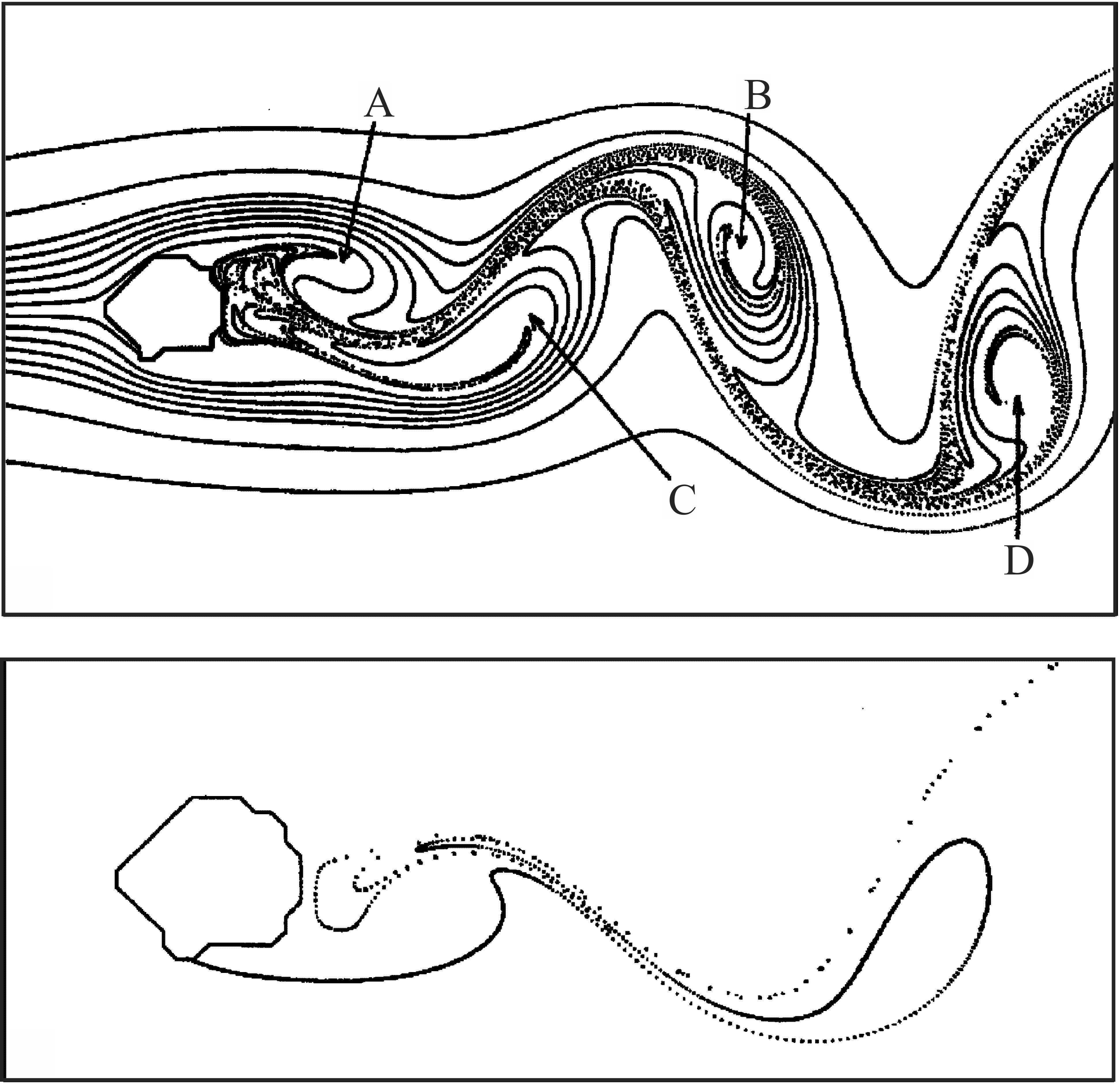
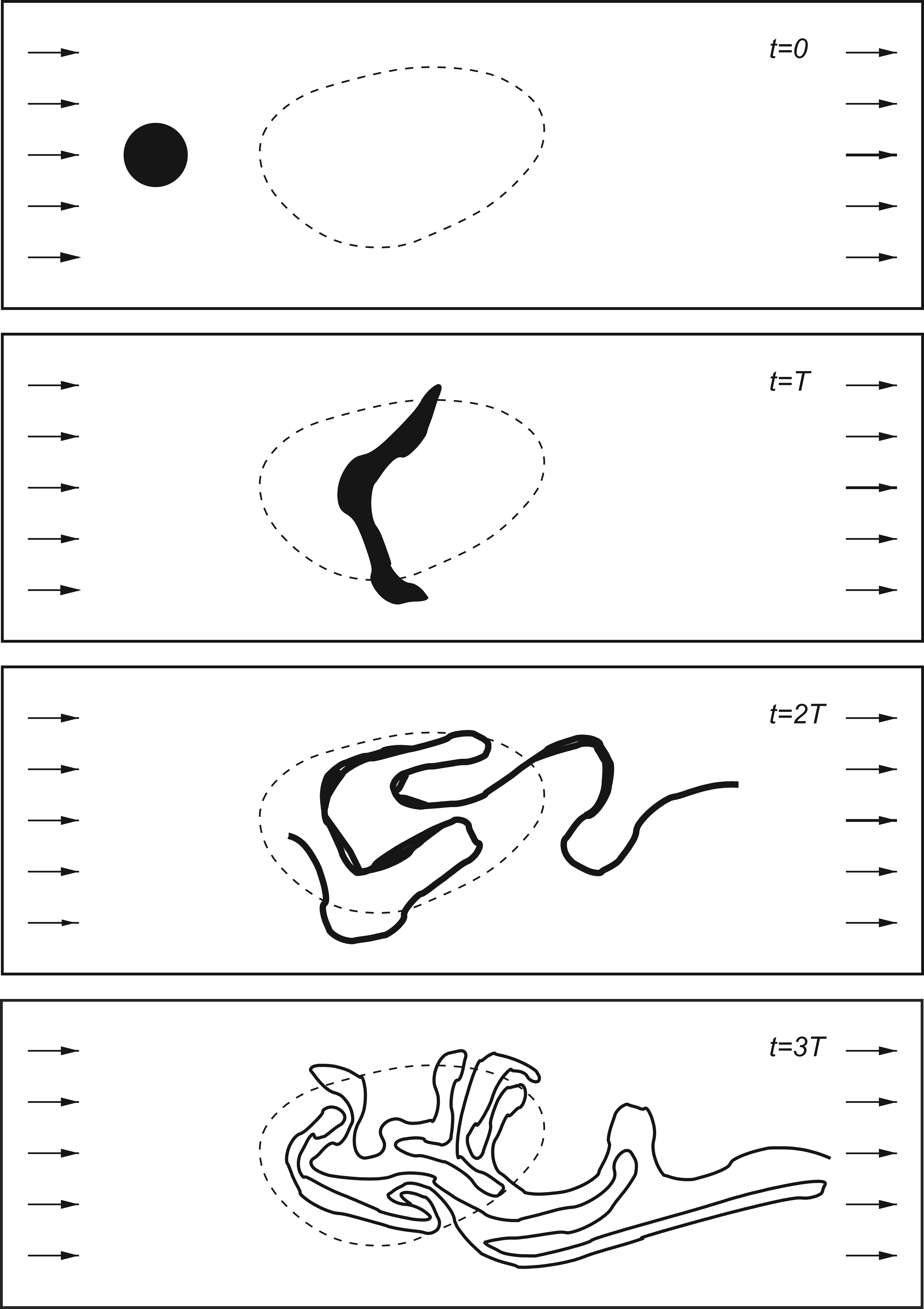
(a)	(b)
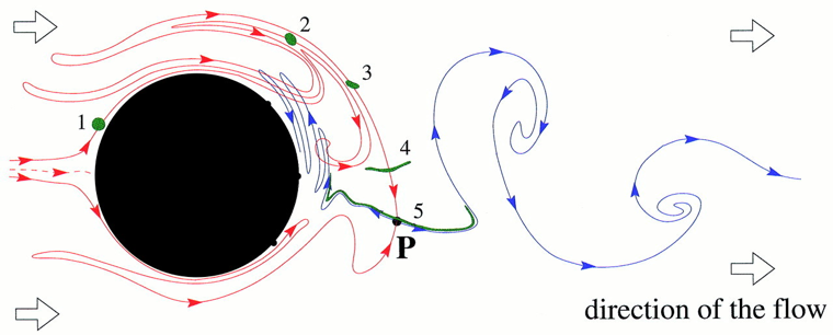
(c)

Figure 3: (a) (top) Numerical simulations of particle trajectories within a von Kármán vortex street emanating from Guadalupe Island. Flow reversal due to vortices corresponds to regions indicated by A, B, C, D. (bottom) Some particle orbits have long residence times due to flow reversal (adapted from Arístegui et al. (1997)). (b) Schematic depicting trapping of of some fluid tracer particles within a mixing region (depicted by dotted line) in an open flow with increasing number of flow periods $T$ (adapted from Tél et al. (2005)). (c) Schematic of the evolution of a blob (green) of tracer particles with number of flow periods and the associated stable (red) and unstable (blue) manifolds in the vortex-shedding wake of cylinder. Particles at the periodic point $\mathbf{P}$ remain trapped there indefinitely (adapted from Károlyi et al. (2000)).

As shown in Figure 3(b, c), the mixing region of an open flow contains the intersection of the stable and unstable manifolds of the flow. The stable manifold is a temporally periodic (due to periodicity of the flow) material line which is comprised of fluid tracer particles which approach the mixing region and get “trapped” within this region for arbitrarily long times ($t\rightarrow\infty$). Whilst this appears to violate conservation of mass, this manifold has zero area, and so particles have a zero probability of lying on it. Despite this, the stable manifold has profound impacts upon transport as the residence time of particles near the stable manifold diverges to infinity the closer a particle is to the stable manifold. Similar to the stable manifold, the unstable manifold (shown in Figure 3(c)) is a material line comprised of fluid particles which approach the mixing region as time goes backward, and so get trapped within this region in the limit $t\rightarrow-\infty$. As illustrated in Figure 3(b), fluid tracer particles close to the unstable manifold eventually leave the mixing region, and so the unstable manifold can be directly observed in open flows by placing a “blob” of fluid particles over the stable manifold. Once this blob enters the mixing region, many particles are swept downstream out of the mixing region; the remainder are trapped locally near the unstable manifold. The remaining particles continue to leak out with time, forming a locus that closely approximates the unstable manifold.

The particles which remain trapped in the mixing region lie close to the chaotic saddle, a fractal set of points which never leave the mixing region. As shown in Figure 3(c), the points which comprise the chaotic saddle are formed by the intersections of the stable and unstable manifolds. These intersections generate continual stretching and folding of fluid elements  (the hallmark of chaotic dynamics, Ottino, 1989) in the chaotic saddle, leading to chaotic advection and exponential stretching of fluid elements within the mixing region.

It is the interplay of flow reversal and open flow that generates the complex mixing and transport dynamics that cannot exist in steady or isotropic Darcy flow. Specifically, the mixing regions of such reversing flows generate chaotic advection which leads to rapid mixing and homogenisation, whilst the chaotic saddle traps neighboring fluid particles for arbitrarily long times. In addition, the mixing region can also admit non-mixing “islands” which (in contrast to the chaotic saddle) are of non-zero area, and so can trap finite amounts of fluid for infinitely long times. All of these dynamics lead to strongly anomalous transport. Conversely, steady Darcy flows are topologically simple (i.e. they have well-defined streamlines and streamsurfaces) and cannot have stagnation points, hence flow reversal in periodic discharge systems is a marked departure from mixing and transport in steady systems. In the remainder of this paper we seek to understand the prevalence of flow reversal in tidally forced aquifers and the impacts on mixing and transport. Using the numerical model described in Section 4.3 we study the Lagrangian kinematics of these flows and consider the implications for anomalous transport.

4 Non-dimensionalization of the governing equations

In order to address the study of Lagrangian kinematics we need to generate accurate solutions to tidally forced groundwater systems. In principle any groundwater flow package can be used to solve the governing equations (9)–(11), but extra care must be taken to assure that accurately cyclo-stationary solutions satisfy the periodic equation in (9). The finite-difference algorithm of Trefry et al. (2009) is second-order convergent and efficiently provides direct solutions (i.e. without time stepping) for both steady and periodic equations. Input parameters to the solution algorithm are the $K$ distribution, the imposed regional flux gradient $J$, the tidal amplitude $\textsl{g}_{p}$, the modal frequency $\omega$, the storativity $S$, and the reference porosity $\varphi_{\textrm{ref}}$. It is useful to non-dimensionalize the governing equations and identify the key dimensionless parameters, which are summarised as follows.

4.1 Dimensionless parameters

4.1.1 Heterogeneity model

The choice of $K$ distribution deserves some discussion. Characterization and representation of physically realistic conductivity fields is a non-trivial task and since the early work of Delhomme (1979) a variety of geostatistical inversion techniques have been developed to make best use of the often sparse field measurements (see for example Deutsch and Journel, 1992; Ezzedine et al., 1999; Fienen et al., 2009). In contrast, in the present work we seek to identify transferable attributes of tidally forced flows, so our emphasis is on understanding how simple models of spatial heterogeneity may potentially contribute to enhanced mixing processes. Our expectation is that if enhanced mixing is detected in simple fields, then similar mixing dynamics will likely also appear in more sophisticated, better-conditioned (and more representative) geostatistical fields. Thus we restrict attention to random spatial processes governed by Gaussian autocorrelation functions, where the mean ($K_{\textrm{eff}}$), log-variance ($\sigma^{2}_{\textrm{log}K}$) and integral scale ($\lambda$) are sufficient to describe the statistics.

4.1.2 Townley number $\mathcal{T}$

Townley (1995) shows that the dimensionless Townley number $\mathcal{T}$ captures the relative timescales of diffusion $\tau_{D}=L^{2}/D_{\textrm{eff}}$ and tidal forcing $\tau_{T}=1/\omega$ in a finite tidal aquifer as

$$\mathcal{T}\equiv\frac{\tau_{D}}{\tau_{T}}=\dfrac{L^{2}S\omega}{K_{\textrm{eff}}}=\dfrac{2\pi L^{2}}{D_{\textrm{eff}}P}$$ (16)

where $D_{\textrm{eff}}\equiv K_{\textrm{eff}}/S$ is the effective aquifer diffusivity. As is well understood for homogeneous aquifers (see following sections), low values of $\mathcal{T}$ provide conditions conducive to propagation of tidal signals far into the aquifer with low phase lags, while high $\mathcal{T}$ values ensure rapid attenuation (damping) of tidal amplitudes and phase lags growing rapidly with increasing penetration distance. Here, for convenience, we are interested in systems where $\mathcal{T}$ is large enough to ensure that finite-aquifer effects are negligible in the tidal forcing zone.

4.1.3 Tidal strength $\mathcal{G}$

We also characterise the relative strength of the tidal forcing amplitude $\textsl{g}_{p}$ to the inland regional gradient $J$, thereby defining the tidal strength

$$\mathcal{G}\equiv\frac{\textsl{g}_{p}}{JL},$$ (17)

such that $\mathcal{G}=0$ corresponds to conventional steady discharge to a constant fixed head boundary. From (9), (10) $\mathcal{G}=\langle||\mathbf{q}_{p}||\rangle/\langle||\mathbf{q}_{s}||\rangle$ in the limit of slow forcing $\omega\rightarrow\infty$, where the angle brackets denote a spatial average over the flow domain. Hence the tidal strength $\mathcal{G}$ controls the propensity for flow reversal over a forcing cycle. Indeed, it can be shown numerically that the product of tidal strength and aquifer log-conductivity variance

$$\mathcal{G}\,\sigma^{2}_{\log K}=\frac{g_{\text{p}}}{JL}\,\sigma^{2}_{\log K},$$ (18)

is strongly correlated with the density of canonical flux ellipses in the tidally active zone, where $\mathcal{G}\,\sigma^{2}_{\log K}=0$ corresponds to flow in aquifers with homogeneous hydraulic conductivity or zero tidal forcing.

4.1.4 Tidal compression ratio $\mathcal{C}$

The final main dimensionless parameter is the tidal compression ratio which characterises the relative change in porosity of the aquifer from its reference state ($\varphi_{\textrm{ref}}$, $h_{\textrm{ref}}$) under a pressure fluctuation of the same magnitude as the tidal forcing amplitude ($\Delta h=\textsl{g}_{p}$), i.e.

$$\mathcal{C}\equiv\frac{\varphi-\varphi_{\textrm{ref}}}{\varphi_{\textrm{ref}}}=\frac{S\textsl{g}_{p}}{\varphi_{\textrm{ref}}},$$ (19)

such that $\mathcal{C}=0$ corresponds to an incompressible aquifer and $\mathcal{C}\ll 1$ corresponds to a weakly compressible aquifer. These limits shall prove useful in understanding how chaotic mixing arises in strongly compressible aquifers, i.e. $\mathcal{C}\lesssim 1$.

The dimensionless parameter set $\mathcal{Q}\equiv(\mathcal{T},\mathcal{G},\mathcal{C})$ controls the dynamics of a periodically forced tidal aquifer. In combination with the set of statistical parameters $\chi$ which define the dimensionless hydraulic conductivity field (where for the log-Gaussian conductivity field in this study $\chi=(\sigma^{2}_{\ln K},\lambda)$), this parameter set completely defines the dimensionless transient tidal forcing problem and so these parameters serve as model inputs. In this way, the set of dynamical parameters $\mathcal{Q}$ can then be translated between aquifer models with different conductivity structures (as defined by $\chi$).

4.2 Heterogeneity characters $\mathcal{H}_{t}$ and $\mathcal{H}_{x}$

In addition to the input parameters sets $\mathcal{Q}$ and $\chi$ there also exist two characteristic dimensionless parameters, $\mathcal{H}_{t}$ and $\mathcal{H}_{x}$, that are functions of the input parameters. These heterogeneity characters are completely defined by $\mathcal{Q}$ and $\chi$ and aid understanding of how the aquifer transport dynamics relate to the heterogeneous structure of the conductivity field.

The heterogeneous flow is governed by the interaction of two physical processes with independent time scales. First, through the imposed regional gradient the inland part of the domain displays a mean drift velocity $v_{\textrm{drift}}\equiv-K_{\textrm{eff}}J/\varphi_{\textrm{ref}}$ toward the tidal boundary where the fluid ultimately discharges. Fluid parcels advecting within this mean drift sample successive $K$ heterogeneities on a time scale of $t_{\textrm{drift}}=\lambda/|v_{\textrm{drift}}|=\lambda\varphi_{\textrm{ref}}/K_{\textrm{eff}}|J|$. Second, the tidal boundary oscillates with period $P$. We define the temporal character of the heterogeneous flow, $\mathcal{H}_{t}$, as the ratio of the drift time scale to the tidal period, i.e. $\mathcal{H}_{t}\equiv t_{\textrm{drift}}/P=t_{\textrm{drift}}\omega/2\pi$. When $\mathcal{H}_{t}\ll 1$ the system is said to be discharge dominated and the groundwater flow displays minimal lateral (longshore) deflections and residence time variances scale with $\sigma^{2}_{\textrm{log}K}$. For $\mathcal{H}_{t}\gg 1$ the system is tidally dominated with low drift velocity: although fluid parcels experience many tidal periods during the journey to the discharge boundary, lateral deflections of the flow paths are suppressed due to the low velocity. Where $\mathcal{H}_{t}\approx\mathcal{O}(1)$ the system is in temporal resonance and there is maximum potential for local elliptical velocity orbits to induce folding of flow paths and the development of chaotic structures.

We also introduce the spatial character of the heterogeneous flow, $\mathcal{H}_{x}$, as a measure of the density of heterogeneities in the tidally affected zone. We define the tidally affected zone as the zone from the tidal boundary to the interior point, $x_{taz}$, where the amplitude of the tidal oscillation ($g_{p}$) matches the mean local steady head, i.e. $|h_{p}(x_{\textrm{taz}},t)|=h_{s}(x_{\textrm{taz}})$. $h_{p}$ can conveniently be estimated using a one-dimensional homogeneous model (Townley, 1995), fixing $x_{\textrm{taz}}$ independently of the heterogeneous numerical solution. The relevant analytical solutions are

$$h_{s}(x)=xJL\>;\>h_{p}(x,t)=\textsl{g}_{p}\>\textrm{cosh}\left[(x-1)\sqrt{i\>\mathcal{T}}\right]\>\textrm{sech}\left[\sqrt{i\>\mathcal{T}}\right]e^{i\omega t},$$ (20)

which are easily established by integration (Trefry et al., 2011). It is straightforward to show that $x_{\textrm{taz}}$ is the root of

$$\mathcal{G}\sqrt{\frac{\cos\left((x_{\textrm{taz}}-1)b\right)+\cosh\left((x_{\textrm{taz}}-1)b\right)}{\cos\left(b\right)+\cosh\left(b\right)}}-x_{\textrm{taz}}=0,$$ (21)

where $b=\sqrt{2\mathcal{T}}$. We define the spatial character by $\mathcal{H}_{x}\equiv x_{taz}/\lambda$, which expresses the number of spatial correlation scales of $K$ that fit within the width of the tidally affected zone (perpendicular to the boundary). The higher $\mathcal{H}_{x}$, the greater the number of conductivity contrasts encountered by the discharging flow while subject to strong elliptical motions.

4.3 Scaled equations and solution approach

4.3.1 Dimensionless model

Based on these physical parameters, we write the governing equations (9)-(10) in dimensionless form via the rescalings $\mathbf{x}^{\prime}=(x^{\prime},y^{\prime})=\mathbf{x}/L=(x/L,y/L)$, $h^{\prime}=h/(JL)$, $t^{\prime}=t\omega$, $\kappa=K/K_{\textrm{eff}}$ yielding the non-dimensional governing equations (where primes are henceforth dropped)

$$\nabla\cdot(\kappa\nabla h_{s}(\mathbf{x}))=0, \nabla\cdot(\kappa\nabla h_{p}(\mathbf{x}))-i\mathcal{T}h_{p}(\mathbf{x})=0,$$ (22)

and non-dimensional boundary conditions on $\mathcal{D}$ (now the unit square)

$$h_{s}(1,y)=1, h_{s}(0,y)=0, h_{p}(1,y)=0, h_{p}(0,y) =\mathcal{G}.$$ (23)

The parameter set $(\mathcal{T},\mathcal{G})$ governs the dimensionless Darcy flux $\mathbf{q}^{\prime}=\mathbf{q}/(JK_{\textrm{eff}})$. Conversely, the tidal compression ratio $\mathcal{C}$ governs scaling of the dimensionless velocity as

$$\mathbf{v}^{\prime}=\mathbf{v}\frac{\varphi_{\textrm{ref}}}{JK_{\textrm{eff}}}=\mathcal{C}\mathbf{q}^{\prime}.$$ (24)

The Lagrangian kinematics are governed by the dynamical parameter set $\mathcal{Q}\equiv(\mathcal{T},\mathcal{G},\mathcal{C})$.

4.3.2 Lagrangian particle tracking

Given solution of (22), (23) via the finite difference (FD) method described in Trefry et al. (2011), the Darcy flux $\mathbf{q}$ and fluid velocity $\mathbf{v}$ are computed via (3) and (14), respectively. To probe the Lagrangian kinematics of these flows, we integrate the advection equation (15) for many passive fluid tracers over many millions of periods of the flow. As shall be shown, in conjunction with the tools and techniques of measure-preserving dynamical systems (chaos theory), such analysis in the Lagrangian frame allows a clear visualisation of the transport dynamics that may not be otherwise apparent.

We require interpolated values of the Darcy flux and fluid velocity for locations away from the FD grid that exactly satisfy (22), as even minor errors violate the measure-preserving nature of the system and lead to spurious results (discussed below). Whilst the FD method computes (22) to within machine precision with respect to the FD stencil (which approximates the differential operators in (22)), interpolated (off-grid) values of $\mathbf{q}_{s}(\mathbf{x},t)$ and $\mathbf{q}_{p}(\mathbf{x},t)$ do not exactly satisfy the continuous differential operators of the governing equations. From the continuity equation (2), the steady Darcy flux $\mathbf{q}_{s}(\mathbf{x})$ must be exactly divergence free, and, as described in Appendix A, we developed a spline interpolation streamfunction representation of $\mathbf{q}_{s}(\mathbf{x})$. The periodic flux $\mathbf{q}_{p}(\mathbf{x},t)$ also must individually satisfy the continuity equation (2); this is achieved by interpolating $\mathbf{q}_{p}(\mathbf{x})$ from the FD grid and then computing the periodic contribution to the porosity $\varphi_{p}$ from the divergence of $\mathbf{q}_{p}(\mathbf{x})$, also described in Appendix A. By constructing q and $\varphi$ in this manner we ensure the solution obeys the continuity equation exactly and the subsequent velocity $\mathbf{v}$ conserves mass to machine precision at all interior locations. This is absolutely critical for the long-term integration of particle trajectories (via (15)) and analysis of Lagrangian characteristics because even tiny violations of mass conservation can lead to serious errors such as spurious sources and sinks in the flow domain and violation of Lagrangian topology (Ravu et al., 2016).

5 Fundamentals of tidal flows in heterogeneous domains

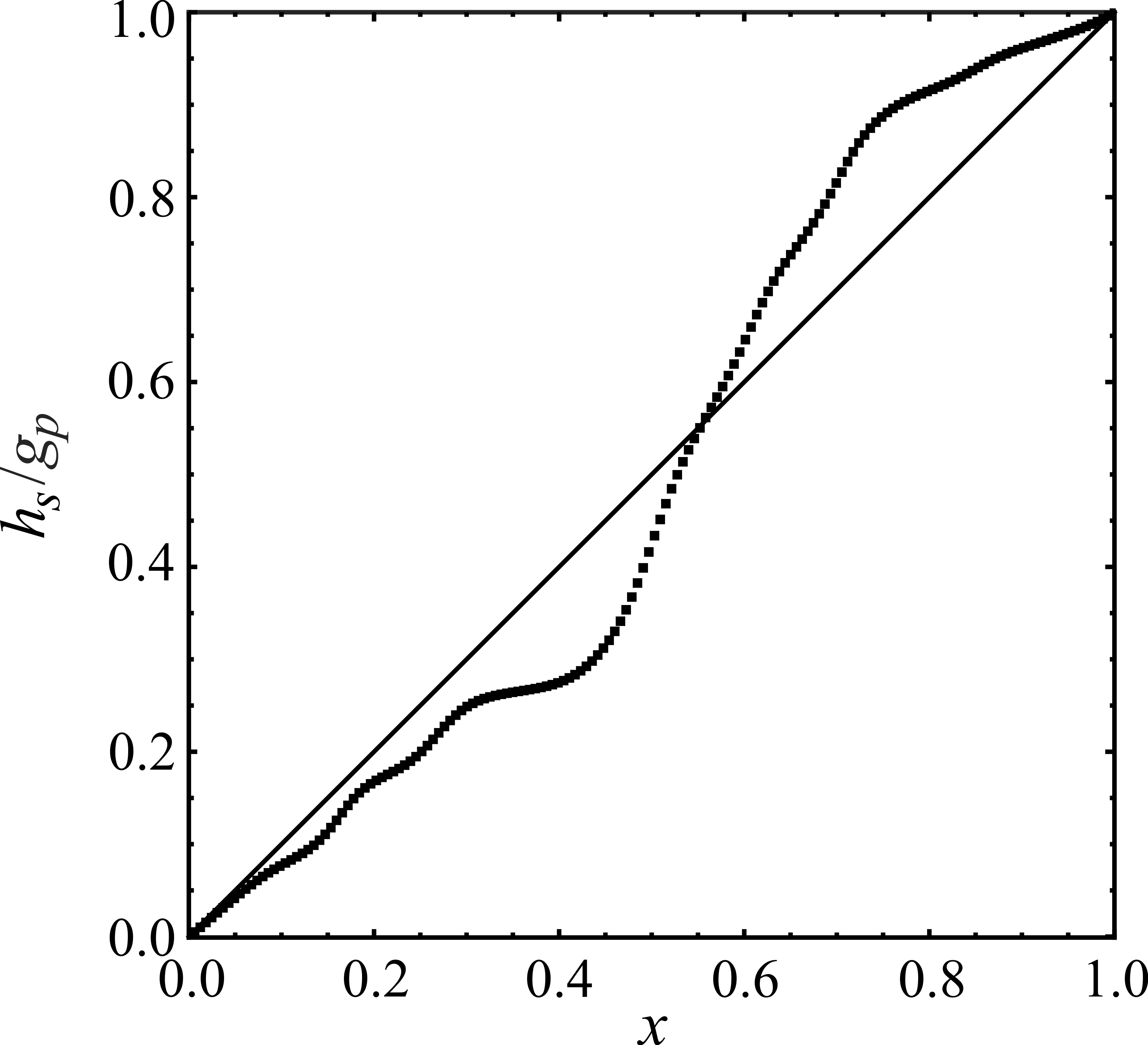
(a)	(b)
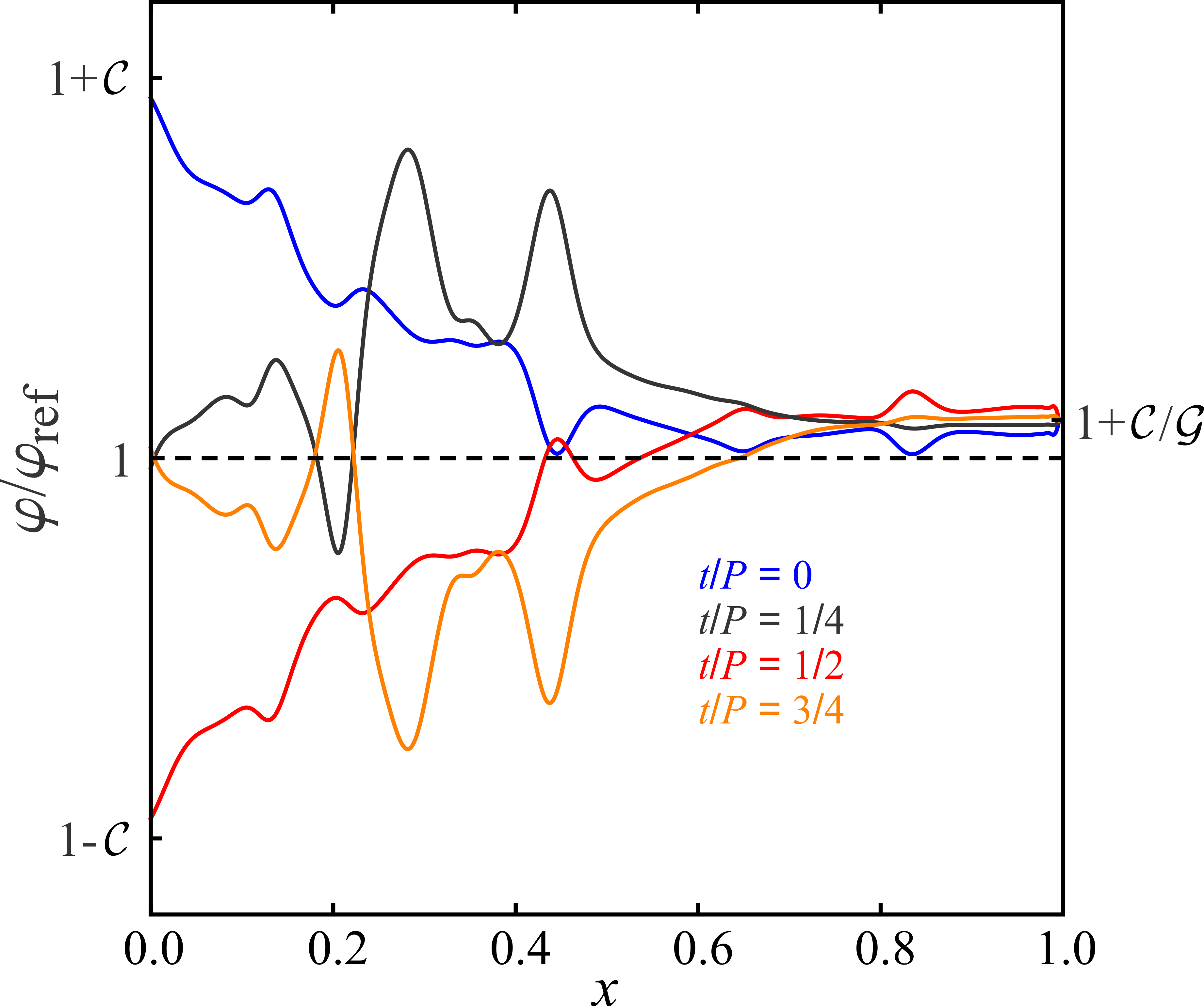
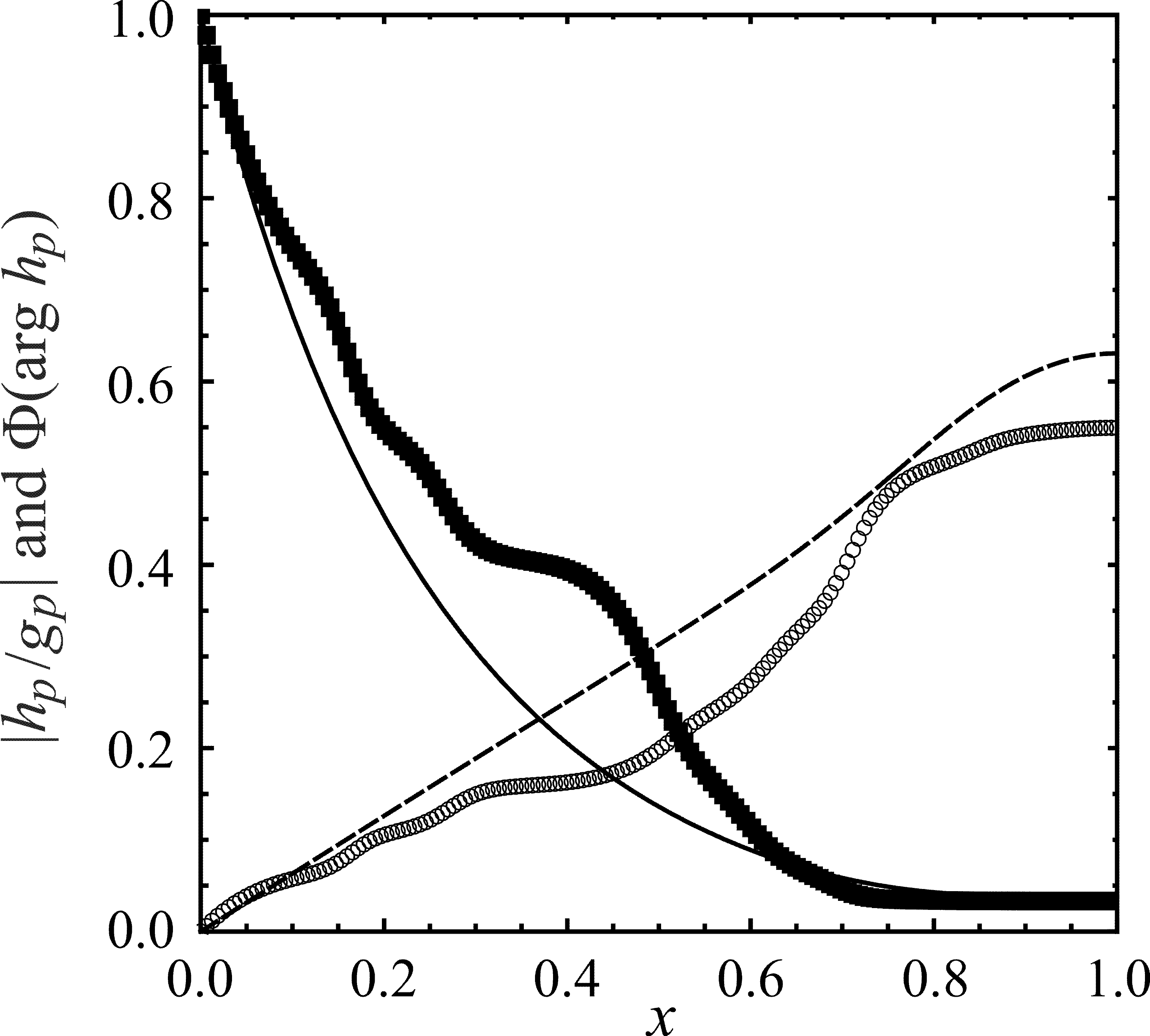
(c)	(d)

Figure 4: (a) Density map of log hydraulic conductivity $\kappa$ where lower (higher) values are darker (lighter). (b) Profile of the steady head $h_{s}$ for the heterogeneous simulation (squares) and reference homogeneous solution (line) along the green line $y$=0.5 shown in (a). (c) Variation of the normalized total porosity $\varphi/\varphi_{ref}$ along $y$=0.5 over the tidal cycle. (d) Same as for (b) but showing the periodic head solution $h_{p}$ (square) and phase lag $\arg h_{p}$ (circles) for the heterogeneous simulation with the reference homogeneous solutions shown as curves.

In this study we focus on the Lagrangian kinematics of the tidally forced groundwater system described in Section 4.3 with parameter set $(\mathcal{T},\mathcal{G},\mathcal{C})$ = (10$\pi$, 10, 0.5) which corresponds to a highly compressible and diffusive aquifer system subject to a diurnal tidal signal. In Section 7.2 we place this parameter set in context with field studies. In subsequent studies we shall explore the distribution of Lagrangian kinematics over the coastal aquifer parameter space $\mathcal{Q}=\mathcal{T}\times\mathcal{G}\times\mathcal{C}$. The hydraulic conductivity field $\kappa$ used is a single $(164\times 164)$ realization generated according to the algorithm of Ruan and McLaughlin (1998) corresponding to an aquifer of moderate heterogeneity ($\lambda=0.049,\sigma^{2}_{\textrm{log}\kappa}=2$). This field yields reversal number $\mathcal{G}\,\sigma^{2}_{\log K}=20$ and heterogeneity characters $(\mathcal{H}_{t},\mathcal{H}_{x})=(4.9,13.6)$, i.e. the system is near temporal resonance and has $\mathcal{O}(10)$ correlation scales within the tidally active zone. The $\kappa$ field is shown in Figure 4, along with the associated steady and periodic head components and evolution of the porosity profile over a forcing cycle. These plots clearly show an exponential decay oscillation amplitude with distance from the tidal boundary for both heterogeneous and homogeneous aquifers, along with a phase lag that increases with distance. Fluctuations in the heterogeneous head solutions away from the homogeneous state have spatial scales that are somewhat larger than $\lambda$ (Trefry et al., 2011). As shown in Figure 4d, the normalized porosity ($\varphi/\varphi_{\textrm{ref}}$) oscillates around unity (with amplitude $\mathcal{C}$) synchronously with the tidal condition at the left boundary, and tends to a value determined by the upstream boundary head $\varphi/\varphi_{\textrm{ref}}\rightarrow 1+JLS/\varphi_{\textrm{ref}}=1+\mathcal{C}/\mathcal{G}$ as $x\rightarrow 1$.

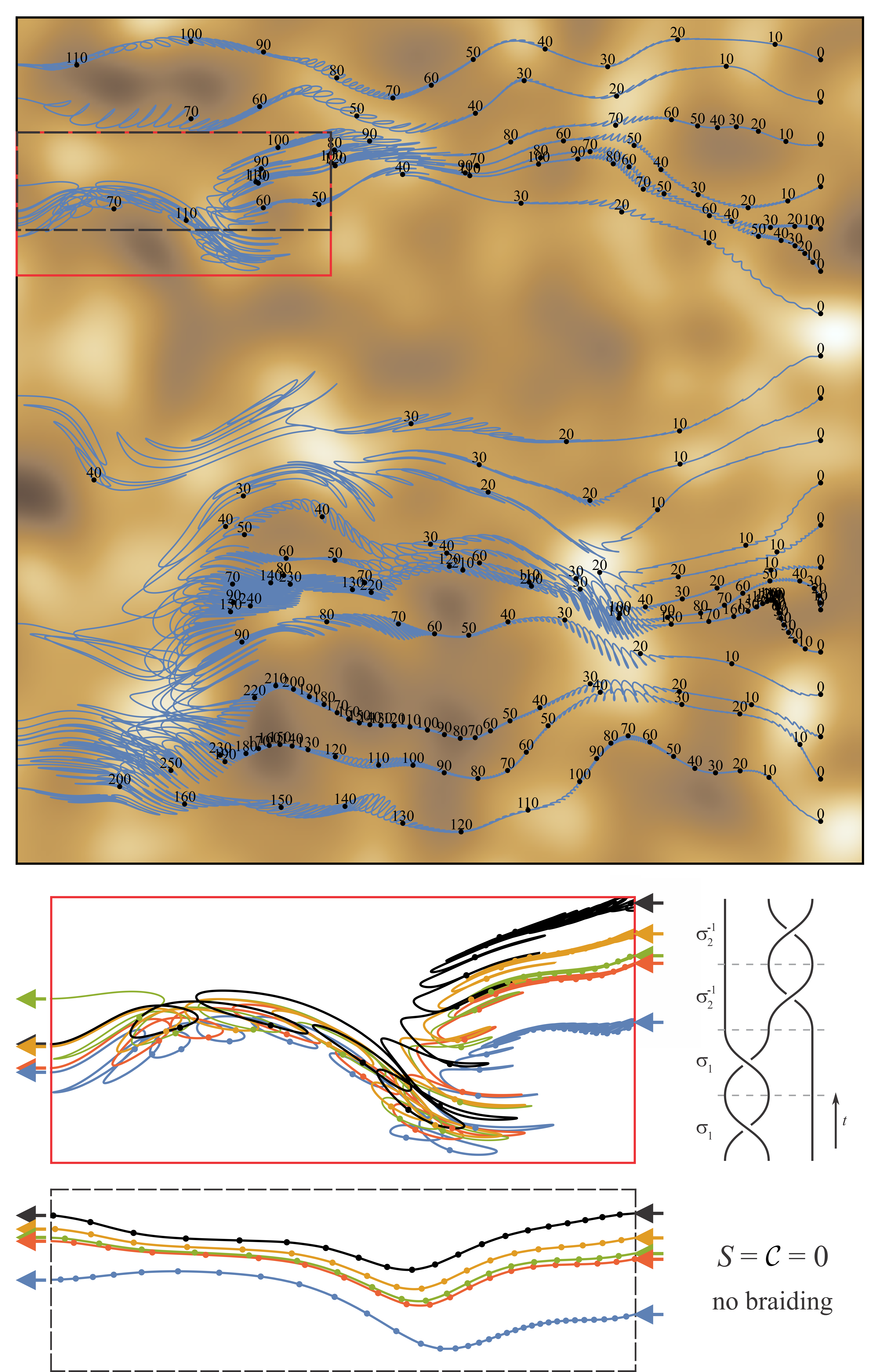
Figure 5: (top) Flow paths, with the number of flow periods shown along each trajectory. (middle left) Detail of the red box with flow paths coloured and dotted every period. Note the change in vertical order of the flow paths from entry to exit (braiding). (middle right) Schematic of generic braiding of fluid trajectories with time $t$ (adapted from Finn and Thiffeault (2011)). (bottom) Corresponding flow paths for the zero-compression case – no braiding is possible (see Appendix D).

Of primary interest are the flow paths shown in Figure 5 which are calculated from a set of equally spaced starting locations near the inland boundary $x=1$; the elapsed number of flow periods is annotated along each flow path. As expected, the spatial heterogeneity of $\kappa$ causes significant deflections of flow paths around low conductivity zones, and travel speeds also vary greatly along and between flow paths. In addition, as the paths move closer to the tidal boundary they encounter flow reversal cells, causing some paths to undergo many sweeps back and forth (flow reversals) with relatively slow net progress toward the tidal boundary. Such flow reversal can result in braiding of particle trajectories, as clearly evidenced by the different vertical ordering of the trajectories at the left and right boundaries in Figure 5 (bottom left). Note that such braiding and transient “crossing” of streamlines can be a signature of chaotic mixing, but this is not possible in steady 2D or in incompressible Darcy flows.

Recent studies (Finn and Thiffeault, 2011; Thiffeault, 2010) have shown that symbolic representation of the braiding motions shown in Figure 5 (lower right) allow the complexity of the braiding motions to be calculated (in terms of the so-called topological entropy), which provides an accurate lower bound for the Lyapunov exponent that characterises chaotic mixing. Trivial braids, such as two sequential crossings that cancel each other out have zero complexity, indicating non-chaotic kinematics. Although not evaluated here, the orbits shown in Figure 5 (bottom left) indicate non-trivial braids with positive complexity and hence chaotic dynamics.

6 Mechanisms and measures of complexity

As seen in the previous section, flow paths for the heterogeneous tidal problem can become entwined and generally present a complicated picture that may obscure the underlying dynamical structures. In this section we seek methods to elucidate and quantify the structure of the tidal discharge map.

6.1 Flow reversal ellipses

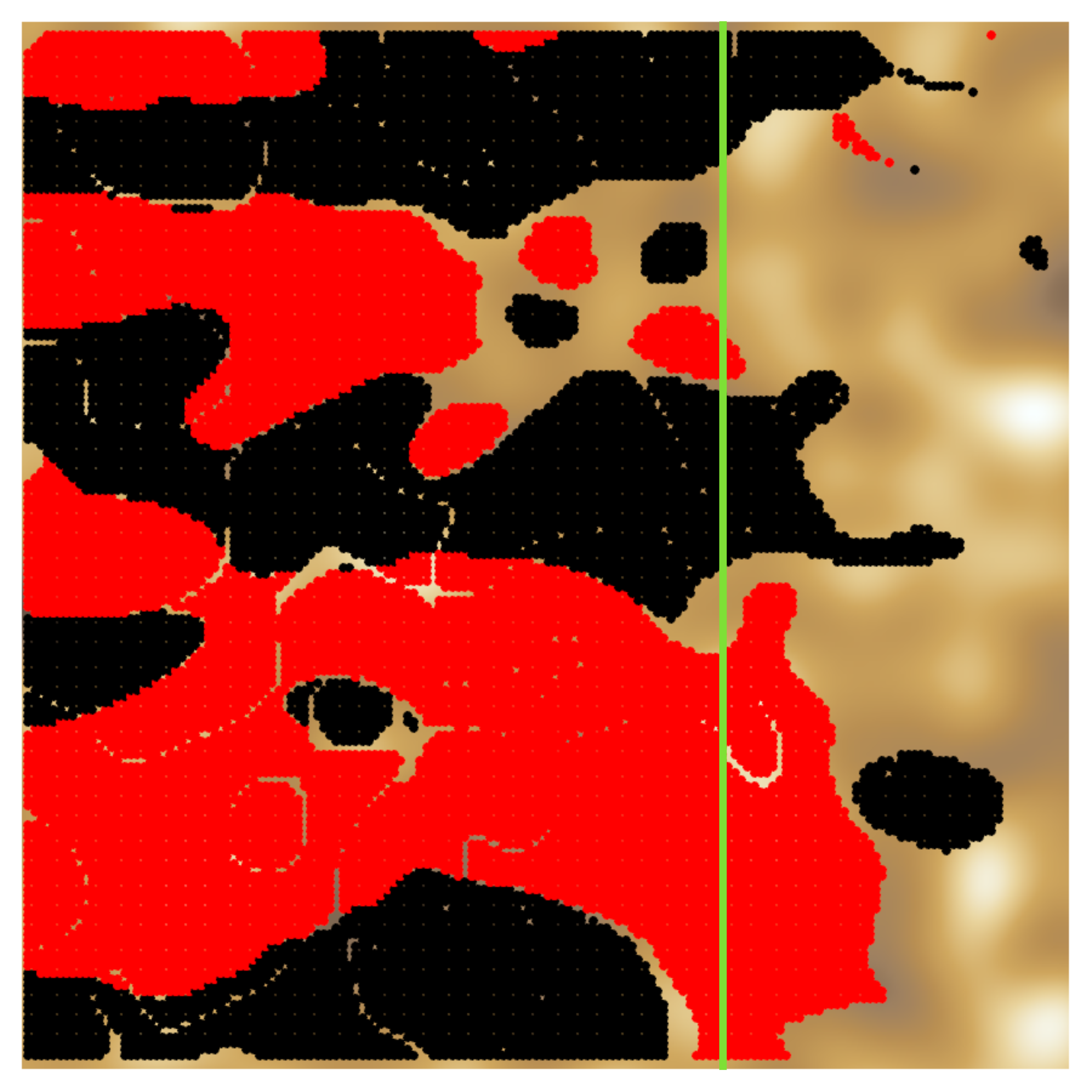
Figure 6: Location of clockwise (black) and anticlockwise (red) canonical flux ellipses (red/black points) evaluated over the aquifer domain. The edge of the canonical flux ellipse distribution approximates the extent of the tidally active zone shown by the green line drawn at $x=x_{\textrm{taz}}$.

Figure 6 shows that almost all of the tidally active zone undergoes flow reversal, where the distribution of flow reversal ellipses in the model aquifer domain is dense near the tidal boundary, and these ellipses appear to extend into the aquifer domain with mean distance similar to $x_{\textrm{taz}}$. The distribution of ellipse rotation (clockwise/anti-clockwise) is also heterogeneous, and is spatially correlated with a somewhat larger integral scale than the underlying hydraulic conductivity field. Whilst flow reversal is directly involved in the generation of complex Lagrangian kinematics (as discussed in Section 6.4.3), we find little correlation between the distribution of flow reversal ellipses and their orientation and the Lagrangian topology of the flow which is discussed throughout this section. Lack of correlation between Eulerian flow measures (e.g. flow reversal) and Lagrangian kinematics and topology is characteristic of chaotic flows and highlights the necessity of visualising transport in the Lagrangian frame.

6.2 Residence time distributions

Transport characteristics of coastal aquifers are primarily quantified in terms of the residence time distribution (RTD) associated with transport of fluid particles through the aquifer. Figure 7(a) shows the RTD ($\tau$) for $10^{4}$ fluid particles seeded in a flux-weighted distribution along the inland boundary ($x=1$) for a steady discharge flow (blue curve), $\mathcal{G}=0$, and for the transient tidal flow (black dots and grey lines), $\mathcal{G}>0$. Figure 7(b) shows a map of the RTD for the transient tidal flow plotted as a function of initial position for a $1000\times 1000$ grid of fluid particles seeded across (center) the aquifer domain $\mathcal{D}$ and (right) a square region covering the largest mixing region of the flow.

The steady regional flow RTD shown in Figure 7(a, blue curve) is continuous and consists of well-defined peaks and troughs that are controlled solely by the heterogeneity of the conductivity field. Conversely, the tidal RTD displays some regions with well-defined, smooth, continuous peaks and troughs, but also other zones of apparently stochastic nature where residence times vary abruptly. Highly resolved plots (not shown) of these residence times indicate they are indeed smooth, but at very small scales. These stochastic zones are interpreted as intervals where neighbouring flow paths are braided (entwined), as demonstrated in Figure 5(a), so that adjacent discharges at the tidal boundary may originate from widely separated flow paths with very different travel times.

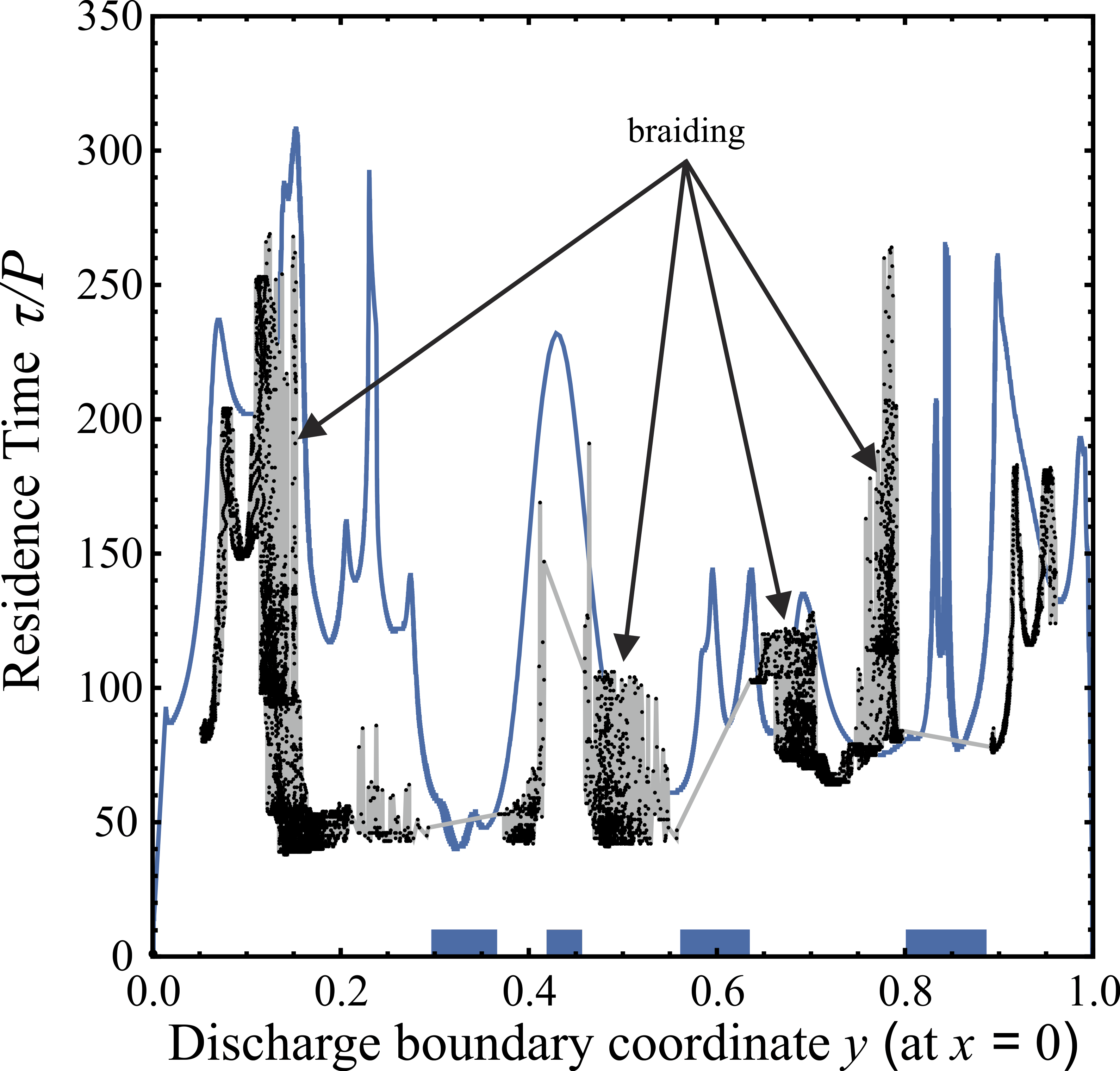
(a)

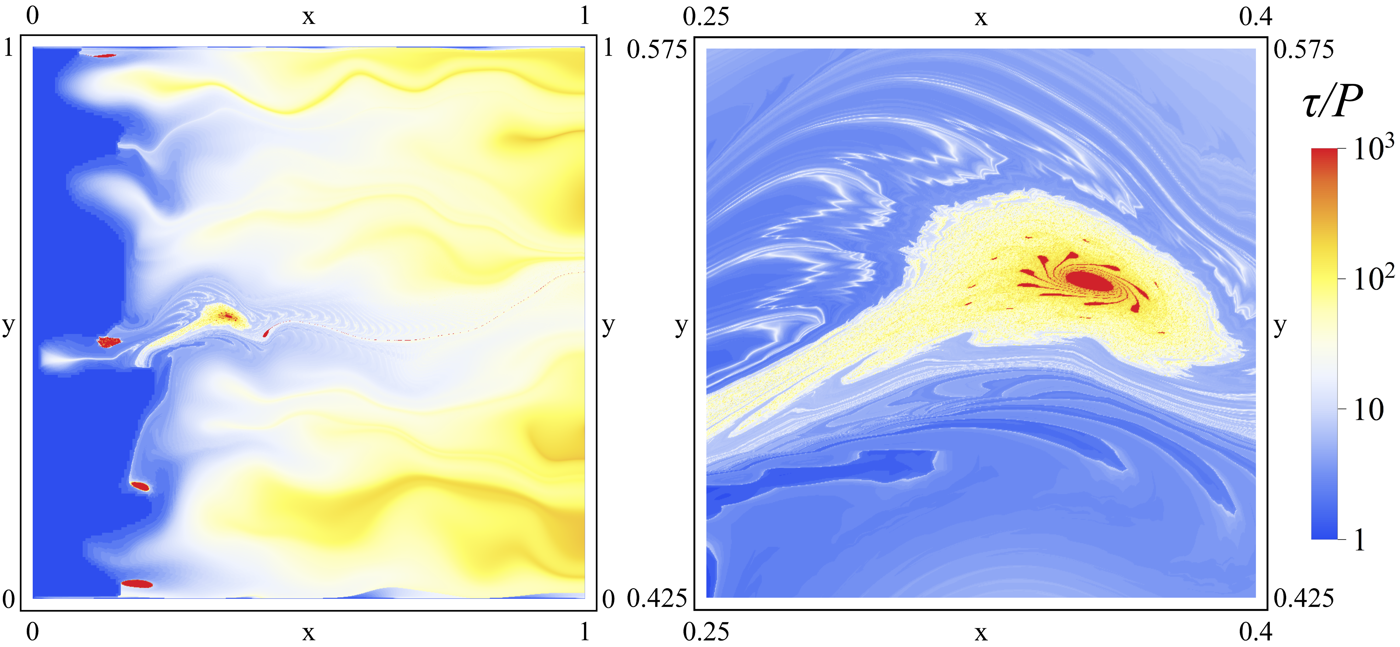
(b)

Figure 7: (a) The blue curve shows the RTD for the steady regional discharge flow, and the black dots indicate residence times for the tidally forced flow. Blue bars indicate zones excluded to regional discharge. Several zones of braided tidal discharge are noted. (b) Maps of RTD for the transient tidal flow plotted in terms of initial position for a $1000\times 1000$ grid of particles seeded over (left) the entire tidal domain and (right) a square region covering the structure centered at $(x,y)\approx(0.35,0.51)$. Particle tracking is performed up to $t/P=10^{3}$, hence red points have residence time $\tau>10^{3}P$.

The tidal RTD appears to be discontinuous at the macroscale in that there are large gaps in the discharge boundary position shown in in Figure 7(a). These are indicated by straight grey lines between black points in the RTD trace and the blue bars along the horizontal axis. The RTD gaps correspond to ”exclusion zones” along the tidal boundary ($x=0$), through which inland flow originating at the inland boundary never exits. Rather, the inland flow discharges in the gaps between these exclusion zones. This unexpected result means that the combination of tidal forcing with aquifer heterogeneity can lead to significant intervals of the tidal boundary being inaccessible to the discharge of regional flow. Below we offer a tentative explanation for the existence of exclusion zones.

Note that the RTD for particles seeded along the inland boundary ($x=1$) for the transient tidal flow (or steady regional flow) do not exhibit diverging residence times (even when much higher resolution of the RTD distribution is computed than that shown in Figure 7(a)), despite observations of such for flow reversal described in Subsection 3.5. This is due to the fact that particles which are seeded at the inland boundary cannot enter these trapping regions for reasons which are explained in Subsection 6.3. Conversely, Figure 7(b) shows that when particles are seeded over the entire flow domain, there are several distinct regions with very long RTDs but which are impervious to particles seeded at the inland boundary. Detail of the largest long RTD “island” indicates a complex, fractal-like structure; the nature and origin of this structure is explained in Section 6.3. The blue region ($\tau\leqslant P$) indicates the set of trajectories that exit the domain within one flow period; we denote this region the tidal emptying region, and the rightmost boundary of this region as the tidal emptying boundary.

6.3 Poincaré sections

The RTD distributions in the previous subsection indicate the presence of complex transport and mixing dynamics within tidally forced aquifers. As indicated by Figure 5, plotting these complex flow trajectories results in a tangle from which it is difficult to discern any coherent structures or Lagrangian topology. A useful tool to aid such visualisation for periodic flows is the Poincaré section, which allows direct visualisation of the Lagrangian topology of the flow field and interpretation of the Lagrangian kinematics within each topologically distinct region. A Poincaré section is formed by tracking a number of fluid particles via the advection equation (15), and recording all particle positions at every time period $\mathcal{P}$ of the flow. The computation does not re-inject particles; once a particle exits the domain it is removed from the simulation. This stroboscopic map essentially “filters out” all of the rapid particle motions between tidal forcing periods, leaving only the slow mean particle motion over each forcing period. Henceforth we shall refer to the flow averaged over a forcing period as the slow flow of the aquifer. It can be shown that fluid transport in periodic flows can almost be completely understood solely in terms of this slow flow, hence Poincaré sections unveil the hitherto hidden transport structure of the aquifer. This approach resolves the Lagrangian topology of the flow into “regular” (i.e. non-chaotic) regions of the flow (with smooth, ordered particle paths) and chaotic mixing regions (with seemingly random particle locations).

(a) Steady flow solution

(b) Full tidal solution

Figure 8: Poincaré sections of regional discharge flux calculated with $\mathcal{P}$=P for steady and for tidal flow cases. The tidal section also shows discharging points in green, calculated with $\mathcal{P}$=P/10 from the particle locations at the last completed tidal period before discharge.

Figure 8 shows two Poincaré sections generated by releasing over 3,000 particles along a vertical line near the inland boundary $(x=1)$ for (a) the steady regional flow and (b) the transient tidal flow. The structure of the Poincaré section for the steady flow arises solely from heterogeneity of the aquifer, where focusing of particles into (away from) high (low) permeability regions is apparent (see, e.g. Trefry et al., 2003), along with differences in advective speed through these high/low permeability regions. Whilst the Poincaré section of the tidal flow is almost identical to that of the steady flow in the vicinity of the inland boundary, significant deviations occur near the tidal boundary. Most apparent is a large region (the tidal emptying region, where $\tau<P$) near the tidal boundary which is devoid of fluid tracer particles seeded from the inland boundary. Within this tidal emptying region there may be subregions where tracer particles may be (i) discharged in times less than a flow period (a discharge region), (ii) enter from outside the aquifer domain ($x<0$) (an entry region), or (iii) are trapped within a subregion indefinitely (a trapped region).

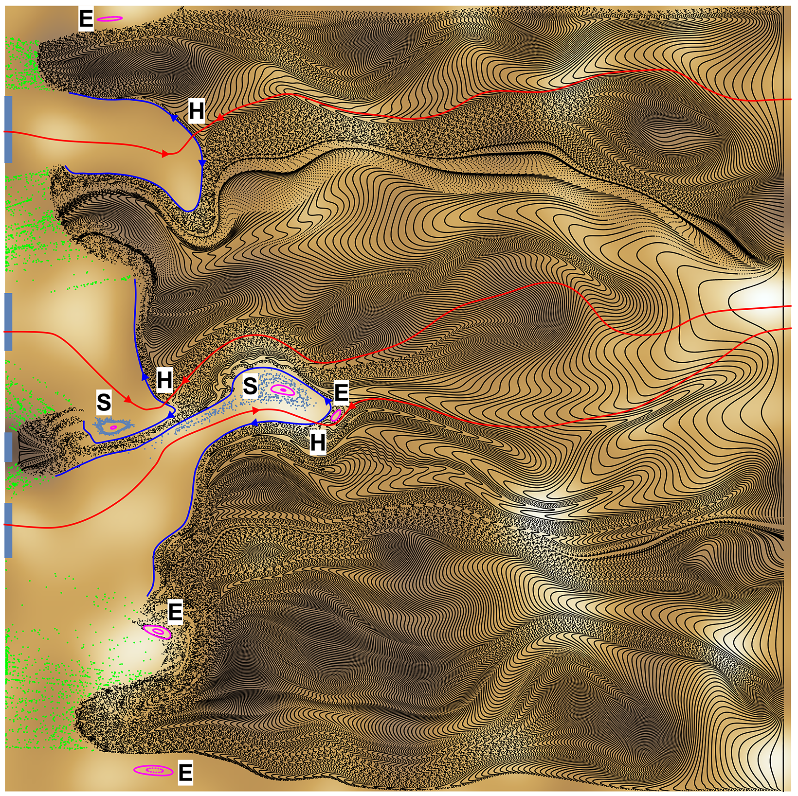
Figure 9: Poincaré section of tidally forced aquifer showing hyperbolic (H) and elliptic (E) points, stochastic layers (S), stable (red lines) and unstable (blue lines) manifolds, KAM islands (magenta orbits), discharge points (green points) and exclusion zones (blue bars).

Discharge regions are clearly illustrated by the green points in Figure 8(b), which indicate the locations of particles that originated from the inland boundary ($x=1$) within the tidal region at temporal increments of $t=P/10$. As shown, discharge along the tidal boundary ($x=0$) coincides with gaps in the exclusion zones shown in the RTD plot in Figure 7(a). This indicates that the exclusion zones along the tidal boundary are associated with the inflow of particles from the oceanic side of the tidal boundary ($x<0$, not modeled). Although the dynamics in these discharge regions appear to be rich (as indicated by the green points in Figure 9), we do not consider them further in this study. Exclusion zones correspond to the blue bars and gaps in the outflow RTD shown in Figure 7(a), and which themselves correspond to inflow regions into the tidal emptying region.

When compared with the residence time distribution plot in Figure 7(b), the tidal region appears to be mainly (but not completely) comprised of particle initial positions with residence times that are either less than one period ($\tau<P$) or have diverging residence time ($\tau\rightarrow\infty$). The short residence time regions indicate discharge or entry regions, whilst the diverging residence times indicate trapped regions within the tidal flow system.

6.4 Elucidation of Lagrangian kinematics and Lagrangian topology

Whilst these observations give a qualitative picture of the complex transport and mixing dynamics in the tidal region, many features are hidden due to selectivity from seeding particles only at the inland boundary $(x=1)$. To resolve the Lagrangian kinematics of the flow fully, in Figure 9 we perform a closer inspection of the Poincaré section by seeding fluid particles throughout the tidal region and resolving Lagrangian coherent structures such as periodic points and invariant manifolds. Here we see, to our knowledge for the first time, how fluid transport due to tidal flows in heterogeneous aquifers is organized and the associated Lagrangian transport structure. These are described in detail as follows.

6.4.1 Periodic points

To clearly elucidate the mixing and transport properties of the aquifer, it is useful to find and classify the structures which control the Lagrangian topology of the flow. To understand these structures it is necessary to introduce key concepts and nomenclature from dynamical systems theory. For periodic flows, key points that organise the Lagrangian kinematics are the periodic points (Ottino, 1989) of the flow, i.e. points that return to the same position after one or more periods of the flow. Points that return after $p$ flow periods are denoted as period-$p$ points, and typically lower-order (e.g. period-1, period-2) points play a greater role in organising transport and mixing. Such periodic points are inadmissible in steady Darcy flow (see Figure 8a), and the presence of periodic points in the tidally forced flow (see Figure 9) is accompanied by a change in the flow topology from open, locally parallel streamlines (Bear, 1972) everywhere to the admission of closed particle orbits and separatrices. Such topological changes bring about vast changes to transport.

Periodic points may be classified in terms of the net local fluid deformation that occurs after $p$-periods; it can be shown in two dimensions that this consists only of either local fluid rotation or local fluid stretching. Periodic points associated with such deformation are termed respectively elliptic (E) and hyperbolic (H) points; the former are associated with non-mixing, regular transport, whereas the latter may be associated with chaotic mixing. As shown in Figure 9, elliptic points are associated with non-mixing “islands” (formally known as KAM islands).

The exclusion zones penetrate far into the aquifer, each terminating at a hyperbolic point (H) at the four-way intersection of associated stable (two) and unstable (two) manifolds. Unstable manifolds (departing blue curves) define the exclusion zone boundaries, while stable manifolds (arriving red curves) act as separatrices for slow fluid trajectories. It is important to remember that whilst structures in the Poincaré section govern the slow flow of particles, complete trajectories of fluid particles include the fast oscillatory motion (as shown in Figure 5) between periods.

The inland stable manifolds divide the regional discharge flow, deflecting to either side of the hyperbolic point. The stable manifolds that intersect the tidal boundary likewise divide the slow flow circulating within the exclusion zone into clockwise or anticlockwise slow motions. The nature of the exclusion zones is now apparent – at high tides water enters the aquifer at the boundary and a fraction of this water performs long excursions into the aquifer, over many tidal periods, moving slowly towards the hyperbolic point before eventually returning to the boundary guided by the nearest unstable manifold. Three separate hyperbolic points are identified in the section, each with their own stable and unstable manifolds. In this way the aquifer contains significant volumes of fluid sourced from the tidal boundary and from the inland boundary; fluids within these two volumes are segregated by the unstable manifolds and do not intermingle until encountering the discharge region (indicated by green points). Note that stable/unstable manifolds cannot terminate in the fluid interior; the unstable manifolds which appear to terminate at the discharge regions in Figure 9 do so as they have not been fully resolved.

6.4.2 Elliptic points

A number of elliptic points (E, enclosed by magenta ellipses) are also identified in the Poincaré section. These occur both within the regional discharge flow and within the exclusion zones. The important dynamical characteristic of elliptic points is that they are surrounded by closed orbits of the slow motion, i.e. the orbits are fixed structures within which fluid circulates perpetually, with infinite residence time. These effects are not reflected in the residence time distributions initiated from the regional flow boundary (Figure 7a) since fluid in the elliptic orbits is never released to the discharge boundary (Figure 7b). The presence of elliptic points also indicates the potential for strong flow segregation in the natural tidal system. Figure 9 shows the presence of elliptic points within the aquifer domain (four labeled E and two associated with stochastic layers), indicating the presence of trapping regions (KAM islands) which hold diffusionless fluid particles perpetually. Even in the presence of diffusion and hydrodynamic dispersion, these finite-sized regions can have a significant impact on solute transport (Lester et al., 2014a).

6.4.3 Chaotic saddles, stochastic layers and cantori

(a)

(b)

Figure 10: (a) Zoomed view of Poincaré section shown in Figure 9, illustrating the stochastic layers (pink dots) and elliptic orbits (red dots) in the mixing regions and regular orbits (blue dots) in the regular regions of the tidal domain. Points are coloured according to residence time, from the least (cyan) to the greatest (red). Roman letters, black and green dots indicate initial positions for FTLE calculations discussed in Subsection 6.5. (b) Detail of Poincaré sections for the mixing regions and surrounding non-chaotic structures in (a) as (black dots), showing points associated with stable (red) and unstable (blue) manifolds, respectively, entering and leaving the aquifer domain via the tidal boundary (green line). The chaotic saddle is the intersection of these manifolds, which surround the elliptic orbits (KAM islands), cantori and stochastic layers.

Two stochastic layers are also identified, labeled by S and indicated by blue points. Each stochastic layer surrounds a set of (magenta) elliptic orbits around an elliptic point (unlabeled). Even though the inner elliptic orbits are perfectly closed, the stochastic layers consist of assemblages of finite orbits where fluid is trapped to circulate the elliptic point for long (e.g. hundreds or thousands of tidal periods) but apparently random circulation times, before being released back into the influence of the nearby unstable manifold for eventual discharge to the tidal boundary. Formally, stochastic layers arise from cantori which are fractal distributions of elliptic points. Figure 10 shows a high resolution Poincaré section focused on the two stochastic layers in Figure 9. This high resolution section provides a much clearer (though still imperfect) picture of the rich dynamical nature of the stochastic layer and associated cantori.

All of the stable and unstable manifolds shown in Figure 9 that organise the basic Lagrangian topology form smooth connections and so do not generate chaotic mixing. However, there also exist transverse intersections between stable and unstable manifolds (such as those shown in Figure 3(c)) that give rise to the chaotic saddles and mixing regions discussed in Section 3.5. Figure 10 show high resolution Poincaré sections focused on the two largest mixing regions shown in Figure 9.

Figure 10(a) shows the stochastic layer (pink points) that surrounds the series of nested elliptic orbits (KAM islands) (red points), and the non-chaotic (regular) regions are denoted by cyan and blue points. These points are coloured with respect to the logarithm of residence time, where cyan/blue points leave the domain after $\mathcal{O}(10)$ periods, pink points $\mathcal{O}(10^{2})$ periods and red points stay within the domain indefinitely. These transport kinematics correspond to the residence time distributions shown in Figure 7(c), where indefinitely-trapped particles in the KAM islands and cantori are surrounded by long-lived (but finite-time) orbits in the stochastic layer.

Figure 10(b) illustrates the stable (red) and unstable (blue) manifolds (shown as discrete points rather than the continuous lines shown in Figure 3(c)). For the aquifer model under consideration, the stable and unstable manifolds respectively enter and leave the aquifer domain via the tidal boundary ($x=0$) rather than having the stable manifold enter from upstream as shown in Figure 3(c). It is presently unknown whether this behaviour is universal to all chaotic saddles in tidally forced aquifers. The chaotic saddle is formed by the transverse intersection of the stable and unstable manifolds which both enter from the tidal boundary $(x=0)$: the stochastic layer is formed by the chaotic mixing dynamics associated with the heteroclinic tangle between the stable and unstable manifolds, which leads to a fractal (spatial) distribution of residence times in the stochastic layer, as described in Section 6.4.3.

The interplay of transient forcing, compressibility and heterogeneity in coastal aquifers leads to complex transport dynamics and a rich Lagrangian topology. Partitioning the Lagrangian topology into distinct regions (which include particle trapping, mixing, particle inflow and outflow) and analysis of the transport within these regions gives an overview of the complex Lagrangian kinematics within tidally forced heterogeneous aquifers. In Section 7.2, we discuss the practical implications of these complex transport dynamics upon solute mixing, transport and chemical reactions.

6.5 Finite-time Lyapunov exponents

Chaotic advection is characterised by the exponential stretching of fluid material elements, where the stretching rate is characterised by the (infinite-time) Lyapunov exponent, defined as

$$\Lambda_{\infty}\equiv\lim_{t\rightarrow\infty}\frac{1}{t}\ln\frac{\delta l(t)}{\delta l(0)},$$ (25)

where $\delta l(t)$ is the length of an infinitesimal fluid line element advected by the flow. A positive Lyapunov exponent $\Lambda_{\infty}>0$ indicates the presence of chaotic advection, and the magnitude of $\Lambda_{\infty}$ indicates the rate of exponential stretching. For closed flows (whether steady or unsteady), the Lagrangian flow domain can be divided into topologically distinct regions which are either regular (non-chaotic, $\Lambda_{\infty}=0$) or chaotic ($\Lambda_{\infty}>0$).

As fluid elements can flow into and out of mixing regions in open flows, it is more useful to characterise deformation of fluid particles in terms of the finite-time Lyapunov exponent (FTLE, $\Lambda$) which quantifies the maximum (i.e. maximum over all possible initial orientations) deformation of an infinitesimal fluid line element (see Appendix C for details). In the limit of infinite residence time the FTLE of an orbit converges to the infinite-time Lyapunov exponent of the chaotic saddle (which does not flow out of the mixing region), which is also equivalent to the ensemble average of the FTLE over many orbits over finite time.

Figure 11: Finite-time Lyapunov exponents calculated from five arbitrarily chosen starting locations in the stochastic layer (see Figure 10). All traces eventually exit at the tidal boundary, except trace F (KAM orbit) which does not terminate and was truncated for display. The ensemble mean and standard error bounds are indicated.

Figure 11 provides FTLE traces calculated from arbitrarily chosen starting locations in the large stochastic layer of Figure 10. The FTLE traces are noisy at short times but become smoother after several hundred $P$ elapsed time. The stochastic layers circulate fluids entering the domain at the tidal boundary before releasing them for subsequent discharge. The recirculation times form a random process depending on particle starting location. Particles at locations A–E all eventually discharge, whereas particles at F circulate indefinitely ($>10^{3}P$). The finite natures of trajectories A–E cause short-term shifts of the FTLE traces as the escaping particles encounter a finite sequence of different Lagrangian regions on their way to the boundary. Thus the FTLE traces in Figure 11 are not monotonically convergent to limiting values, as is common for evaluations of infinite-time Lyapunov exponents ($\Lambda_{\infty}$). To overcome this estimation problem we calculated FTLE values for a random ensemble of 42 starting locations (green and black dots in Figure 11), gaining an ensemble mean FTLE $\approx 0.149$ with low standard error. For comparison, Lester et al. (2013b) show that pore-scale branching networks lead to an infinite-time Lyapunov exponent of $\Lambda_{\infty}\approx 0.12$. Thus our ensemble of (finite) open flow trajectories in the stochastic layer displays a positive mean FTLE indicative of chaos, while the infinite KAM orbit (F) displays only algebraic $(\Lambda=0)$ deformation.

7 Discussion and physical relevance

Results from the previous sections have clearly established the presence of complex transport phenomena and rich Lagrangian topology in tidally forced aquifers. In this section we consider the impacts of these transport dynamics on transport, mixing and reactions, and we place the example problem in the context of a selection of relevant field studies.

7.1 Implications for transport and reaction

Groundwater discharge is a prime vector for contaminant migration and environmental impact. However it is beyond the scope of this paper to extend our Lagrangian analysis to dispersive/diffusive systems, although this is clearly an important direction for future research. Here we limit our comments to observations of Lagrangian phenomena in our simulations that impinge upon the utility of conventional groundwater quality characterization activities.

7.1.1 Residence time distributions - segregation and singularity

In our example problem we saw that the residence time distribution of fluid in the aquifer domain was singular (infinite) at several locations controlled by periodic points. Furthermore, regional flux was diverted into several discrete discharge zones along the tidal boundary, and the fluids discharging in these zones had undergone complicated braiding dynamics which may mix and mask geochemical signatures. At other locations along the boundary there were intervals of recirculation (with widths of the order of the log-conductivity correlation length $\lambda$) where tidal fluids embarked on long incursions into the aquifer domain, lasting many tidal periods, before eventually returning and discharging at the boundary. Thus, taken as a whole, fluids discharging along the tidal boundary may have vastly different (and possibly indeterminate) geochemical and chronological origins. This behaviour is fundamentally different to the familiar steady discharge dynamics in heterogeneous domains (see the blue curve in Figure 7). Conventional groundwater sampling techniques near discharge boundaries, e.g. multilevel samplers and spear probes, may variously source fluids from an ensemble of histories and qualities. High sampling density, in space and time, may be the best practical defense against these unpredictable effects in poorly characterized aquifers.

7.1.2 Flow reversal and traceability

The origin of these complicated transport dynamics can be traced back to reversal of the Darcy flux vector during the tidal forcing period over a significant proportion of the aquifer domain (see Figure 6), leading to a fundamental change in the Lagrangian topology from open, parallel streamlines to the formation of periodic points, separatices, non-mixing islands and chaotic saddles (see Figures 8, 9). Moreover, our observations of punctuated inflow/outflow regions along the tidal boundary ($x=0$) significantly alter understanding of transport in these regions, especially from the perspective of, for example, salt water intrusion. Such complex transport dynamics are incompatible with many solute transport and biogeochemical reaction modeling studies which tend to rely on the identification of simple mean flow paths along which complicated mass balance and reaction kinetic calculations can be made. Conceptually, our results suggest that determination of the fate (provenance) of reacting fluids simply by (back-) tracking along an approximate steady streamline may well be a source of significant model error in coastal discharge environments. That is, determination of mean fluid flow paths for geochemical reaction modeling and transport may not be appropriate or even possible in some coastal settings. In addition, it has been shown (Tél et al., 2005) that the complex mixing dynamics that arise within chaotic regions can profoundly alter a wide range of chemical and biological reaction rates.

The highly oscillatory nature of particle motion near the tidal boundary (see Figure 5) can also significantly skew estimates of tracer migration speed. Although the net displacement of a particle over a tidal period $P$ may be small, the mid-cycle particle displacement can be much larger. Noting that most tidal spectra are multi-modal and that the Townley number $\mathcal{T}$ is frequency-dependent, the appropriate sampling frequency may be a function of sampling location in the aquifer. It is clear from our results that tracer test analysis in strongly tidally influenced aquifers is potentially fraught.

7.2 Potential for chaos in field settings

Figure 12: Location of the present example system (star) in $\mathcal{T}$ – $\mathcal{G}\,\sigma^{2}_{\textrm{log}K}$ parameter space. Locations of some field studies reported in the literature are provided for reference (see text for details).

It is important to consider how the dimensionless parameter set $\mathcal{Q}$=($\mathcal{T}$, $\mathcal{G}$, $\mathcal{C}$)=(10$\pi$,10,0.5) and conductivity parameters ($\sigma^{2}_{\log K}=2$, $\lambda=0.05$) of our example problem relates to those of typical coastal aquifers. Noting that the product $\mathcal{G}\,\sigma^{2}_{\log K}$ correlates well with the density of canonical flux ellipses in the tidally active zone, in order to assess the relevance of these parameter values to field studies we estimate $\mathcal{T}$ and $\mathcal{G}\,\sigma^{2}_{\log K}$ values from a set of published coastal aquifer studies. The study locations are the Dridrate Aquifer, Morocco (D, sand and limestone) (Fakir and Razack, 2003), Garden Island (GI, sand and limestone) (Trefry and Bekele, 2004), Jervoise Bay (J, sand and limestone) (Smith and Hick, 2001) and Swan River (SR, sand and clay) (Smith, 1999), all in Western Australia, Largs North, South Australia (LN, sand and clay) (Trefry and Johnston, 1998), and Pico Island, Azores (P, basalts) (Cruz and Silva, 2001). Figure 12 plots these studies in $\mathcal{T}$–$\mathcal{G}\,\sigma^{2}_{\log K}$ space with error bars indicating uncertainty in hydrogeological parameter estimates. The GI, SR and J studies include multiple data points due to the use of frequency-resolved techniques. Estimates of $\sigma_{\textrm{log}\kappa}^{2}$ are rare in tidal analyses although suitable estimation techniques exist (see e.g. Trefry et al., 2011). The following ranges of $\sigma_{\textrm{log}\kappa}^{2}$ were assumed: 0.5–2.5 (sand and limestone, sand and clay), 2.0–6.0 (basalts). Figure 12 shows that the example problem (star) lies well within the range of $\mathcal{T}$ values of the field studies but at the upper end of the estimated flow reversal $(\mathcal{G}\,\sigma^{2}_{\log K})$ values.

The tidal compression ratio $\mathcal{C}=S\!_{s}\,g_{\text{p}}/\varphi_{\text{ref}}$ is also a key parameter. As porosity $\varphi_{\textrm{ref}}$ is not always well characterized in tidal aquifer studies, we resort to literature values for soil physical parameters (Domenico and Mifflin, 1965; Morris and Johnson, 1967). For sand and limestone soils, $\varphi_{\textrm{ref}}$ ranges from 0.2–0.5, while for sand and clay soils the range is 0.15–0.4. Basalts, often with significant fracture porosity, may show $\varphi_{\textrm{ref}}$ in the range 0.03–0.35. Specific storages $S_{s}$ typically range up to $10^{-2}\,\textrm{m}^{-1}$ (sand and limestone, sand and clay) and $10^{-4}\,\textrm{m}^{-1}$ (fractured rock), while tidal amplitudes can be as large as 10 m. With these ranges the maximum $\mathcal{C}$ values that can be anticipated are approximately 0.05 (sand and limestone), 0.4 (sand and clay) and 0.02 (basalts), but lower tidal amplitudes will reduce these proportionately. Thus we see that the example problem, with $\mathcal{C}=0.5$, is at the high end of likely values in field settings, closest to a clay and sand matrix influenced by high tidal amplitude. It is beyond the scope of this paper to identify specific instances of Lagrangian chaos in coastal aquifers, but the preceding analysis shows that the parameter choices in the example problem are not far removed from reality and there is good prospect of coherent Lagrangian structures being present near discharge boundaries in many field settings.

However, whether such structures may be detected in field investigations is another matter altogether. Submarine groundwater discharge (SGD) mapping techniques are directly relevant to the detection of Lagrangian structures in coastal systems, but the uncertainties involved in SGD are significant. Firstly, coastal discharge zones often display complex geomorphology, topography and fully three-dimensional heterogeneity at a range of spatial scales. This complexity is sufficient to render the SGD measurement task onerous, even at relatively poor spatial resolution. Once gathered, the measurements show significant spatial and temporal variability due to geological structure, temporal variations in flow regime, and measurement uncertainty. The measurement variability is often rationalized in terms of (unresolved) preferential flow paths (see, for example Hosono et al., 2012; Smith et al., 2003) although other mechanisms including density effects, wave action (Smith et al., 2009) and tidal and weather system influences are also reported to be important (Kobayashi et al., 2017). Our results indicate that tidal forcing introduces a new dynamical mechanism for generating preferential flow paths via the establishment of interior hyperbolic points, resulting in segregation of regional flow into discrete discharge zones. It remains to be seen whether techniques can be developed to isolate the presence and quantify the effects (on flow, mixing and reaction) of Lagrangian structures in coastal systems. Nevertheless, the potential for Lagrangian chaos must be recognized and assessed.

8 Conclusions

In this paper, motivated by earlier studies in coastal groundwater hydraulics and biogeochemical transport, we have considered the dynamics and kinematics of (dispersion-free) flow in a simple 2D time-periodic groundwater discharge system, which represents a broad class of natural (unpumped) hydrogeological environments. Using standard linear poroelastic theory, spectral solutions to the linear Darcy flow equations were obtained using a finite-difference scheme coupled with a self-consistent streamfunction method which resulted in a highly accurate, time-periodic velocity field. Spatial heterogeneity of aquifer conductivity was accounted for explicitly, yielding complex and coupled spatio-temporal variations in head, porosity, flux and velocity.

We have, for the first time, uncovered the underlying transport structure of tidally forced aquifers. Rather than study the advection-diffusion of a passive scalar, we advect diffusionless tracer particles to uncover this non-trivial transport structure. Resolution of the Poincaré section of the example groundwater flow reveals a rich Lagrangian topology, with features that include:

1. Elliptic islands - isolated regions of the flow which trap fluid particles indefinitely

2. Chaotic saddles - isolated regions of the flow which involve rapid mixing and augmented reaction kinetics

3. Flow segregation - division of the flow domain into distinct subdomains

4. Tidal inflow/outflow - division of the tidal boundary into distinct inflow or outflow regions

This complex transport structure has profound ramifications for flow, transport and reaction in time-periodic groundwater discharge systems, and changes our understanding of transport and mixing processes (such as saltwater intrusion) in these systems at a fundamental level. The interplay of this diffusionless transport structure and dispersive processes represents a pressing direction for future research.

We show that the interplay of tidal forcing and aquifer heterogeneity is responsible for these complex Lagrangian kinematics. Specifically it is the presence of flow reversal points in the aquifer that are directly responsible for the change in flow topology from everywhere parallel streamlines (associated with steady Darcy flow) to the presence of closed flow path lines, periodic points and separatrices. This change in flow topology fundamentally alters the transport characteristics of the aquifer, leading to indefinite trapping of fluid elements in circulation regions and segregation of the flow domain into distinct regions.

We also show that non-zero aquifer compressibility can lead to a further topological bifurcation to form chaotic saddles: localised regions of chaotic advection that involve rapid mixing and augmented reaction kinetics. These chaotic regions augment transport and mixing dynamics of the aquifer. Our example problem used a relatively high compressibility value (compared to typical field values) and we are presently scanning the lower compressibility values to determine the parametric extent of this chaotic behaviour.

The results presented in this paper demonstrate that a conventional Darcian groundwater flow system has the potential to admit complex and possibly chaotic flows as long as two preconditions are met: a heterogeneous aquifer domain and at least one time-periodic discharge boundary.

Appendix A Method for self-consistent, physically constrained flows

When considering the dynamical aspects of flow fields, evaluations of velocity vectors for particle tracking purposes require greater accuracy than is commonly provided in many groundwater modeling investigations. This is because the identification of Lagrangian structures can require a combination of long particle travel times and fine spatial resolution. Numerical calculations of the Darcy flux vector at arbitrary locations in the problem domain can be problematic since calculations require both differentiation and interpolation of discretised variables ($\kappa$ and $h$). Here we describe a numerical method to solve for the tidal heads via a finite difference approach, and then generate heads, fluxes and porosities in continuous forms consistent with the relevant physical constraints (2) and (4). These continuous variables allow the fluid velocity field to be evaluated to an accuracy sufficient to support the required analyses of Lagrangian flow characteristics. A Mathematica version 11 notebook containing the full numerical implementation is available from the authors on request.

The steady and periodic head solutions of (22) and (23) calculated according to the numerical scheme in Trefry et al. (2009) are presented as head distributions $h_{s}$ and $h_{p}$ evaluated on a regular (square) finite difference grid with spatial increment $\Delta$. The corresponding flux distributions $\textbf{q}_{s}$ and $\textbf{q}_{p}$ are constructed by finite differences according to

$$\textbf{q}_{s}(\textbf{x}_{m,n}) = \left(-\bm{\kappa}^{+}_{x}\,\left[h_{s}(\textbf{x}_{m+1,n})-h_{s}(\textbf{x}_{m,n})\right],-\bm{\kappa}^{+}_{y}\,\left[h_{s}(\textbf{x}_{m,n+1})-h_{s}(\textbf{x}_{m,n})\right]\right)/\Delta$$

$$\textbf{q}_{p}(\textbf{x}_{m,n},t) = \dfrac{e^{i\omega t}}{\Delta}\left(-\bm{\kappa}^{+}_{x}\,\left[h_{p}(\textbf{x}_{m+1,n})-h_{p}(\textbf{x}_{m,n})\right],-\bm{\kappa}^{+}_{y}\,\left[h_{p}(\textbf{x}_{m,n+1})-h_{p}(\textbf{x}_{m,n})\right]\right)$$

where $m$ and $n$ index the finite difference nodes in the $x$ and $y$ directions, respectively, and $\textbf{x}_{m,n}=(x_{m},y_{n})$. For the present 2D problem the mid-nodal conductivity values may be estimated either by harmonic averages:

$$\bm{\kappa}^{+}_{x} = 2\,\bm{\kappa}_{m+1,n}\,\bm{\kappa}_{m,n}/(\bm{\kappa}_{m+1,n}+\bm{\kappa}_{m,n})$$

$$\bm{\kappa}^{+}_{y} = 2\,\bm{\kappa}_{m,n+1}\,\bm{\kappa}_{m,n}/(\bm{\kappa}_{m,n+1}+\bm{\kappa}_{m,n})$$ (27)

or geometric averages:

$$\bm{\kappa}^{+}_{x} = \sqrt{\bm{\kappa}_{m+1,n}\,\bm{\kappa}_{m,n}}$$

$$\bm{\kappa}^{+}_{y} = \sqrt{\bm{\kappa}_{m,n+1}\,\bm{\kappa}_{m,n}}.$$ (28)

In this work geometric averaging is used exclusively. The flux estimation scheme (A) provides error residuals identical to those of the head solution. The nodal porosity is expressed as

$$\varphi(\textbf{x}_{m,n},t) = \varphi_{\textrm{ref}}+S\left(h_{s}(\textbf{x}_{m,n})-h_{\textrm{ref}}+h_{p}(\textbf{x}_{m,n})e^{i\omega t}\right)$$ (29)

$$= \varphi_{s}(\textbf{x}_{m,n})+\varphi_{p}(\textbf{x}_{m,n},t)$$

Consider the continuity equation (2). This must be satisfied at all locations (not just at the finite-difference nodes) and times in the model system in order for fluid mass to be conserved. Noting that, formally, the Darcy flux q and porosity $\varphi$ satisfy (13) and (11), respectively, we see that the continuity equation can be expressed as (involving continuous quantities):

$$\nabla\cdot(\textbf{q}_{s}+\textbf{q}_{p}e^{i\omega t})+\dfrac{\partial(\varphi_{s}+\varphi_{p}e^{i\omega t})}{\partial t}=0$$ (30)

Expanding this equation and noting the time-independence of the results yields the following two identities for exactly mass-conserving flow in our model periodic system:

$$\nabla\cdot\textbf{q}_{s}=0$$

$$\nabla\cdot\textbf{q}_{p}+i\omega\,\varphi_{p}=0.$$ (31)

This result shows that the periodic component of the Darcy flux induces a bounded oscillation in the local porosity which, in turn, modulates the advective velocity via (11). It is usual to generate continuous Darcy flux distributions by interpolating between the finite-difference nodal fluxes. If, however, our interpolated estimate of the steady Darcy flux component is not precisely divergence-free, i.e. $\nabla\cdot\textbf{q}_{s}=\epsilon\neq 0$, where $\epsilon$ is independent of time, then the continuity equation becomes

$$\dfrac{\partial\varphi}{\partial t}=-\nabla\cdot(\textbf{q}_{p}\,e^{i\omega t})-\epsilon$$ (32)

which provides for unbounded growth of $\varphi$ as $t\rightarrow\infty$, resulting in unphysical flow paths. To remedy this situation we impose equations (A) as exact constraints on the interpolated numerical solutions for q and $\varphi$ via the following three-step process.

Step 1: Enforcing zero divergence for $\textbf{q}_{s}$ via a streamfunction approach

Consider the steady component of the Darcy flux, $\textbf{q}_{s}$, with nodal values $\textbf{q}_{s;m,n}=(\textbf{q}^{x}_{s;m,n},\textbf{q}^{y}_{s;m,n})$ and continuous vector interpolation $\textbf{q}^{\text{int}}_{s}(x,y)=(w_{x}(x,y),w_{y}(x,y))$. Even if $\textbf{q}^{\text{int}}_{s}$ exactly reproduces the numerical fluxes at the finite-difference node points it does not follow that the interpolation necessarily provides zero divergence at all locations $(x,y)$. We address this by constructing an effective streamfunction, $\Psi$, for $\textbf{q}_{s}$ based on $\textbf{q}^{\text{int}}_{s}$ and then differentiating $\Psi$ to generate modified flux components $\textbf{q}^{\ast}_{s,x}$ and $\textbf{q}^{\ast}_{s,y}$ according to

$$\textbf{q}^{\ast}_{s,x}\equiv\dfrac{\partial\Psi}{\partial y}\enskip,\quad\textbf{q}^{\ast}_{s,y}\equiv-\dfrac{\partial\Psi}{\partial x}.$$ (33)

This results in an explicitly divergence-free flux distribution since

$$\nabla\cdot(\textbf{q}^{\ast}_{s,x},\textbf{q}^{\ast}_{s,y})\equiv\dfrac{\partial^{2}\Psi}{\partial x\,\partial y}-\dfrac{\partial^{2}\Psi}{\partial y\,\partial x}=0.$$ (34)

The effective streamfunction is calculated by integrating the interpolation $\textbf{q}^{\text{int}}_{s}$ according to (33) over the finite difference grid, yielding the two datasets:

$$\Psi^{(x)}_{m,n} = \int_{y_{0}}^{y_{n}}q^{\text{int}}_{s,x}(x_{0}+m\Delta,y^{\prime})dy^{\prime},$$

$$\Psi^{(y)}_{m,n} = -\int_{x_{0}}^{x_{m}}q^{\text{int}}_{s,y}(x^{\prime},y_{0}+n\Delta)dx^{\prime}.$$ (35)

where each integral is performed by quadrature over $N_{knots}$ points. These datasets are combined to provide two independent estimates of the streamfunction $\Psi$ over the finite difference grid as

$$\Psi^{(1)}_{m,n} = \Psi^{(x)}_{m,n}+\Psi^{(y)}_{m,0},$$

$$\Psi^{(2)}_{m,n} = \Psi^{(y)}_{m,n}+\Psi^{(x)}_{0,n}.$$ (36)

Rather than choose between these estimates, we assemble the streamfunction in discrete form by the simple average $\Psi_{m,n}=(\Psi^{(1)}_{m,n}+\Psi^{(2)}_{m,n})/2$. The discrete streamfunction $\Psi_{m,n}$ is then converted to final continuous form ($\Psi(x,y)$) via interpolation and the modified flux components calculated via (33).

Step 2: Enforcing the continuity equation on $\textbf{q}_{p}$ and $\varphi_{p}$

In order to ensure that the transient form of the continuity equation (A) is also satisfied, we fix the modified transient porosity component $\varphi_{p}^{\ast}$ by setting $\varphi^{\ast}_{p}(x,y)=-(i\omega)^{-1}\nabla\cdot\textbf{q}^{\text{int}}_{p}(x,y)$, where $\textbf{q}^{\text{int}}_{p}$ is the interpolated transient flux solution based on the finite-difference nodal values for $\textbf{q}_{p}$. The total modified Darcy flux is constructed as $\textbf{q}^{\ast}(x,y,t)=\textbf{q}^{\ast}_{s}(x,y)+\textbf{q}^{\text{int}}_{p}(x,y)\,e^{i\omega t}$ and the total modified porosity as $\varphi^{\ast}(x,y,t)=\varphi^{\text{int}}_{s}(x,y)+\varphi^{\ast}_{p}(x,y)\,e^{i\omega t}$. In turn, the periodic head $h^{\ast}_{p}$ is fixed by (11,13), yielding $h^{\ast}(x,y,t)=h^{\text{int}}_{s}(x,y)+h^{\ast}_{p}(x,y)\,e^{i\omega t}$. Thus, identically, we satisfy the continuity equation and compressibility relation over the problem domain and obtain an exactly mass-conserving velocity field $\textbf{v}^{\ast}=\textbf{q}^{\ast}/\varphi^{\ast}$ that incorporates the underlying tidal groundwater hydraulics.

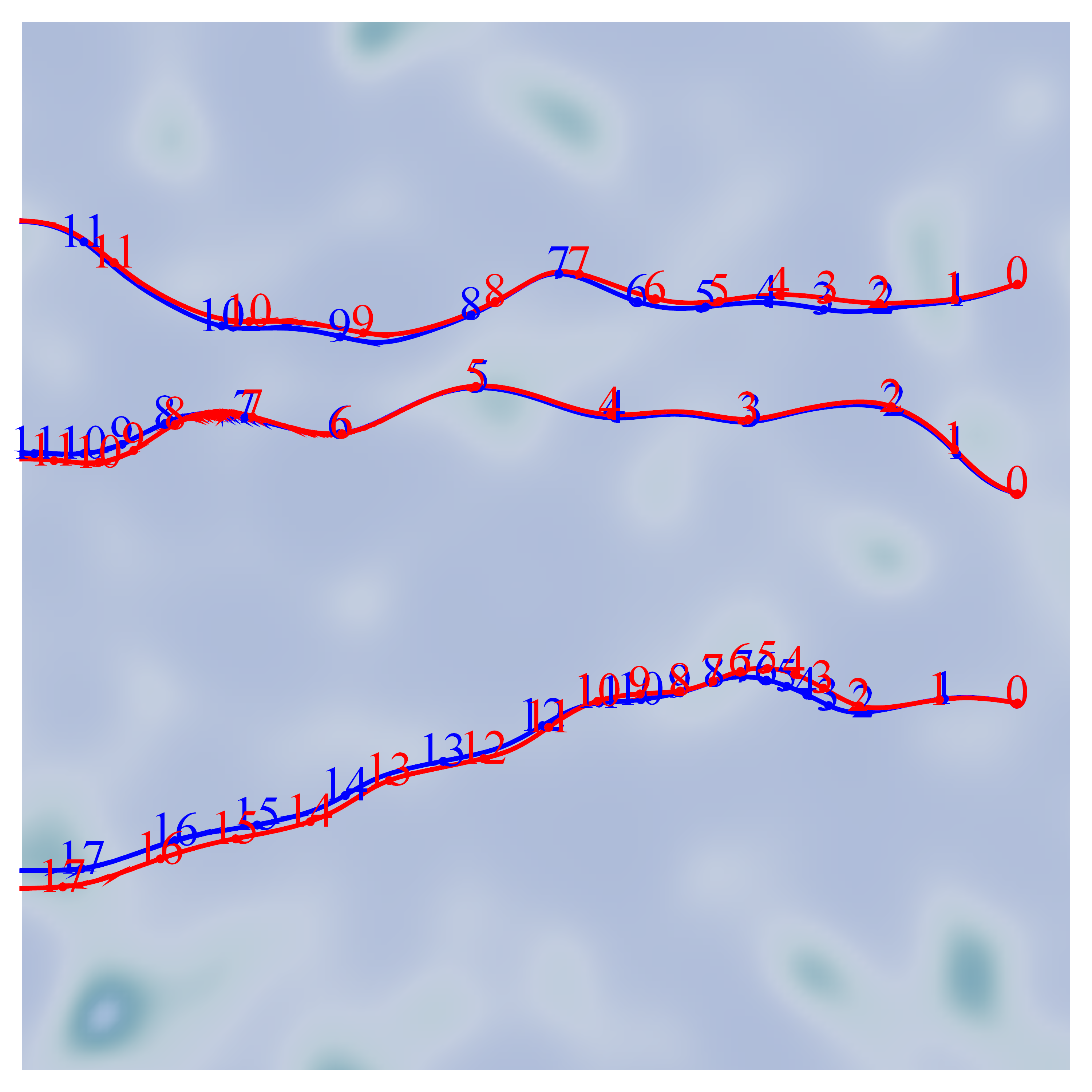
Figure 13: Comparison of flow paths integrated forward in time using simple interpolation of finite-difference solutions (red) and full CE-corrected solutions (blue) superimposed on the associated $\kappa$ field (shaded). Numbering refers to the number of elapsed periods P ($\times 100$) along each path, starting at $t=0$ at the points to the right.

In general the updated variables differ from those interpolated directly from the finite-difference flux solution but retain the character of the underlying numerical solution. Figure 13 compares three arbitrary flow paths calculated using $\textbf{v}^{\text{int}}$ with the counterpart path calculated using $\textbf{v}^{\ast}$ with $N_{knots}=501$.

Step 3: Checking self-consistency of the adjusted dependent variables

The previous two steps have ensured that the updated dependent variables ($h^{\ast},\textbf{q}^{\ast},\varphi^{\ast}$) satisfy the continuity equation and the compressibility relation, but at the cost of perturbing the variables from the finite-difference values. We assess the nature and magnitude of the perturbations using the Darcy equation (3) as a reference. The updated heads and fluxes will be consistent with a Darcian process if the updated flux vector $\textbf{q}^{\ast}$ and the gradient of the updated head $\nabla h^{\ast}$ are aligned. This alignment is tested by calculating azimuths $\theta_{\nabla h^{\ast}}=\textrm{ArcTan}(\nabla h^{\ast}_{y}/\nabla h^{\ast}_{x})$ and $\theta_{q^{\ast}}=\textrm{ArcTan}(q^{\ast}_{y}/q^{\ast}_{x})$ of the updated steady flux and steady head gradient vectors, with zero azimuth chosen to lie in the mean flow direction (negative $x$ direction). Azimuth plots were compiled by sampling the updated head and flux distributions at the finite difference node locations and plotting the sample values against each other, and comparing this with the discrete solution counterpart.

Figure 14: Self-consistency checks of azimuths from steady fluxes and head gradients for the finite-difference solution (left column), interpolated solution (center column) and the updated flux (right column) evaluated for two different correlation lengths (upper and lower rows). The numerical scheme gives better results at larger correlation lengths.

Results of this assessment are shown in Figure 14 for two different spatial correlation lengths $\lambda/\Delta$ and $(N_{x},N_{y})=(64,64)$. In each case the finite-difference solution provides an azimuth plot with non-zero mean discrepancy between the head gradient and flux vectors, which is a consequence of the discrete heads being evaluated at grid nodes (with specified conductivity values) and the discrete fluxes at mid-nodal locations (with spatially averaged conductivity values). The finite-difference azimuth plots provide a lower bound to the error of the updated azimuth distributions. For $\lambda/\Delta=2$ the updated azimuth plot shows wide dispersion, including many samples with opposed azimuths (approximately 15% of the flux and head gradient vectors have opposite flow directions); however, for $\lambda/\Delta=12$ the updated azimuths are more tightly aligned ($<1.4\%$ opposed flows). Figure 15 displays the $\lambda$-dependence of the mean azimuthal discrepancy, showing that the mean azimuth error drops to less than $1^{\circ}$ for $\lambda/\Delta\geq 8$ for $\sigma^{2}_{\textrm{log}\kappa}=1$. The results also depend on the conductivity variance $\sigma^{2}_{\textrm{log}\kappa}$: increasing variances worsen the azimuthal discrepancy.

Figure 15: Dependence of mean azimuthal difference $\overline{\Delta\theta}$ for the updated fluxes on the correlation length $\lambda/\Delta$ of a set of realizations of the input conductivity field with variances $\sigma^{2}_{\textrm{log}\kappa}$ = 1/2 (squares), 1 (dots), 2 (triangles) and 4 (circles). Curves are fitted to each set of points to aid the eye, and the acceptability cutoff is set at $1^{\circ}$ (dashed line).

Fundamentally, the results presented in this Appendix give confidence that our numerical scheme generates Darcian solutions that strictly obey the necessary continuity and compressibility constraints so long as the spatial conductivity variations are sufficiently well sampled (resolved) by the discrete set of input $\kappa$ values. In order to guarantee acceptable quantitative performance of the physical constraints and laws in our simulations it is useful to adopt a maximum permissible mean azimuthal discrepancy, e.g. $1^{\circ}$. In this case, for unit variance $\sigma^{2}_{\textrm{log}\kappa}=1$ attention would be confined to cases where $\lambda/\Delta\geq 8$ as indicated in Figure 15 (see dashed line).

Appendix B Connection of flow reversal to matrix conductivity and poroelasticity

It is clear from Figure 8 that the effect of the tidal boundary is to generate significant flow reversals that stimulate the Lagrangian phenomena of interest. Vorticity provides a measure of flow reversal and can be related to key physical processes in the poroelastic system. Consider the vorticity $\bm{\nu}$ of our 2D groundwater flow, defined by $\bm{\nu}\equiv\mathbf{\nabla}\times\mathbf{v}=\mathbf{\nabla}\times(\mathbf{q}/\varphi)$. By a standard vector identity the curl of a product of a scalar and a vector is, in the notation of our system,

$$\bm{\nabla}\times\left(\frac{\mathbf{q}}{\varphi}\right)=\nabla\left(\frac{1}{\varphi}\right)\times\mathbf{q}+\left(\frac{1}{\varphi}\right)\bm{\nabla}\times\mathbf{q}=\varphi^{-2}\left(\nabla\varphi\times\mathbf{q}\right)+\varphi^{-1}\left(\bm{\nabla}\times\mathbf{q}\right).$$ (37)

Noting that $\nabla\varphi=S\nabla h$ (see equation (4)) and that the curl of the gradient of a scalar is zero results in the vorticity relation

$$\bm{\nu}=\frac{\nabla h\times\nabla\kappa}{\varphi}$$ (38)

expressed in terms of the conductivity and porosity of the matrix. Using the expression for the linear poroelasticity (4) and defining $\hat{h}(\mathbf{x},t)\equiv(h(\mathbf{x},t)-h_{\textrm{ref}})/\textsl{g}_{p}$ as the non-dimensional local forcing, equation (38) becomes

$$\bm{\nu}=\frac{\bm{\nu}_{\kappa}}{1+\mathcal{C}\hat{h}}$$ (39)

with

$$\bm{\nu}_{\kappa}=\frac{\nabla h\times\nabla\kappa}{\varphi_{\textrm{ref}}}$$ (40)

the vorticity from shear flows generated solely by conductivity variations.

Equation (39) implies that flow reversal occurs due to conductivity variations and poroelasticity (if the storativity varies in space, (38) includes an additional term $\kappa h(\nabla h\times\nabla S)$ that could separately generate vorticity due to non-trivial variation of the storage field). The magnitude of $\bm{\nu}_{\kappa}$ is controlled by the conductivity variance $\sigma_{\textrm{log}\kappa}^{2}$. However, as discussed in Appendix D, it is the trajectory symmetry breaking due to poroelasticity that produces interesting Lagrangian transport structure. Flow reversal from non-trivial conductivity variation and symmetry breaking from poroelasticity are the two crucial physical ingredients in the creation of the transport dynamics we observe.

Appendix C Fluid deformation gradient tensor and finite time Lyapunov exponent

Chaotic advection in any fluid flow is characterised by the exponential stretching of fluid material elements, which gives rise to rapid growth of material interfaces, and hence accelerated mixing and transport. This phenomenon is typically characterised by the (infinite-time) Lyapunov exponent (25), but for particle orbits in open flows with finite residence time in the flow domain, it is more useful to characterize deformation in terms of the finite-time Lyapunov exponent (FTLE). To formally define and derive the FTLE $\Lambda$ and the associated fluid deformation gradient tensor $\mathbf{F}$, we first introduce the Lagrangian spatial coordinate system $\mathbf{X}$, which may be defined in terms of the Eulerian trajectory $\mathbf{x}(t,t_{0};\mathbf{X})$ of a fluid particle at position $\mathbf{X}$ at time $t_{0}$. The Eulerian trajectory $\mathbf{x}(t,t_{0};\mathbf{X})$ is a solution of the advection equation

$$\frac{\partial\mathbf{x}}{\partial t}=\mathbf{v}(\mathbf{x},t),\qquad\mathbf{x}(t=t_{0},t;\mathbf{X})=\mathbf{X},$$ (41)

and so represents a transformation from Lagrangian ($\mathbf{X}$) to Eulerian ($\mathbf{x}$) spatial coordinates. The FTLE is computed from the fluid deformation gradient tensor $\mathbf{F}(t,t_{0};\mathbf{X})$ which quantifies how the infinitesimal vector $d\mathbf{x}(t,t_{0};\mathbf{X})$ deforms from its reference state $d\mathbf{x}(t=t_{0},t_{0};\mathbf{X})=d\mathbf{X}$, and so represents the Jacobian tensor associated with a transformation from Lagrangian to Eulerian coordinates:

$$d\mathbf{x}=\mathbf{F}\cdot d\mathbf{X},$$ (42)

and, equivalently,

$$F_{ij}\equiv\frac{\partial x_{i}}{\partial X_{j}}\qquad\textrm{where}\qquad\mathbf{F}\equiv[F_{ij}].$$ (43)

Following this definition, the deformation gradient tensor $\mathbf{F}(t,t_{0};\mathbf{X})$ evolves with travel time $t$ along a Lagrangian trajectory (streamline) as

$$\frac{\partial\mathbf{F}}{\partial t}=\nabla\mathbf{v}\left[\mathbf{x}(t,t_{0};\mathbf{X}),t\right]^{\top}\cdot\mathbf{F}(t,t_{0};\mathbf{X}),\quad\mathbf{F}(t=t_{0},t_{0};\mathbf{X})=\mathbf{1},$$ (44)

where the superscript $\top$ denotes the transpose. We refer to (44) as the evolution equation for $\mathbf{F}$. Given computation of the deformation gradient tensor via, the FTLE is then defined as

$$\Lambda(t,t_{0};\mathbf{X})\equiv\frac{1}{2(t-t_{0})}\ln\nu_{d},$$ (45)

where $\nu_{d}$ is the largest eigenvalue of the right Cauchy-Green deformation tensor $\mathbf{C}$

$$\mathbf{C}=\mathbf{F}(t,t_{0};\mathbf{X})^{\top}\cdot\mathbf{F}(t,t_{0};\mathbf{X}).$$ (46)

Note that in the limit $t-t_{0}\rightarrow\infty$, the FTLE converges to the (infinite-time) Lyapunov exponent $\Lambda_{\infty}$, and due to ergodicity in chaotic regions, the ensemble average $\langle\Lambda(t,t_{0};\mathbf{X})\rangle$ (where the average is performed over many starting positions $\mathbf{X}$) also converges to $\Lambda_{\infty}$. In this way, the infinite-time Lyapunov exponent in for chaotic regions in open flows may be accurately estimated even if the typical orbit residence time is short.

For incompressible flows, $\nabla\cdot\mathbf{v}=0$, (44) yields the result $\det(\mathbf{F})=1$, i.e. the volumes of fluid elements are preserved under the flow. However the groundwater velocity $\mathbf{v}=\mathbf{q}/\varphi$ is not divergence-free, so care needs to be taken in computing the fluid deformation gradient tensor $\mathbf{F}(t,t_{0};\mathbf{X})$ and the associated FTLEs $\Lambda(t,t_{0};\mathbf{X})$ in the linear groundwater flow (5) due to spatio-temporal variability of the porosity $\varphi(\mathbf{x},t)$. Conservation of fluid mass under the linear groundwater flow is captured explicitly by the continuity equation (2) and tracking of fluid “particles” must be performed with respect to the groundwater velocity. Note that whilst the variable nature of $\varphi$ renders neither $\mathbf{v}$ nor $\mathbf{q}$ divergence-free, it is important that constraints imposed by (2) on particle advection kinematics and fluid deformation are enforced so to eliminate spurious transport and mixing behaviours (see Appendix A).

From the evolution equation (44), we find

$$\det\mathbf{F}(t,t_{0};\mathbf{X})=\exp\left[\int_{t_{0}}^{t}\nabla\cdot\mathbf{v}(\mathbf{x}(t^{\prime},t_{0};\mathbf{X}),t^{\prime})\,dt^{\prime}\right],$$ (47)

where the integral is also applied in fixed Lagrangian position $\mathbf{X}$. We derive an explicit expression for the divergence $\nabla\cdot\mathbf{v}$ as follows. We define the fluid material derivative as

$$\frac{D_{f}}{Dt}\equiv\frac{\partial}{\partial t}+\mathbf{v}\cdot\nabla,$$ (48)

and so from (2),

$$\nabla\cdot\mathbf{v}=-\frac{D_{f}}{Dt}\ln\varphi,$$ (49)

hence

$$\det\mathbf{F}(t,t_{0};\mathbf{X})=\exp\left[\int_{t_{0}}^{t}-\frac{D_{f}}{Dt^{\prime}}\ln\varphi\,\,dt^{\prime}\right]=\frac{\varphi(\mathbf{X},t_{0})}{\varphi(\mathbf{x}(t,t_{0};\mathbf{X}),t)}.$$ (50)

The impact of mass conservation (2) is that the volume of a moving fluid element scales inversely with the local porosity $\varphi$. Whilst this imposes temporal fluctuations in $\det\mathbf{F}$, these are transient and bounded, hence mass is conserved over arbitrarily long times. As such (50) serves as a consistency check during particle tracking and computation of FTLEs.

Appendix D Integrability of particle trajectories for incompressible media

To show that fluid particle trajectories are integrable for incompressible media (i.e. they cannot exhibit chaotic dynamics), we consider the linear groundwater equation (5) in the limit $S=0$ in terms of the steady $h_{s}(\mathbf{x})$ and periodic $h_{p}(\mathbf{x},t)$ head solutions

$$\nabla\cdot\left(K(\mathbf{x})\nabla[h_{s}(\mathbf{x})+h_{p}(\mathbf{x},t)]\right)=0,$$ (51)

subject to the fixed head boundary conditions $h|_{x=L}=\textsl{g}_{L}$, $h|_{x=0}=\textsl{g}(t)$, the latter of which may be decomposed into steady and zero-mean fluctuating components as $\textsl{g}(t)=\bar{\textsl{g}}+\textsl{g}^{\prime}(t)$. Due to linearity (51) is satisfied individually by the steady and periodic solutions, which may be expressed as

$$h_{s}(\mathbf{x}) = \textsl{g}_{L}+(\bar{\textsl{g}}-\textsl{g}_{L})f(\mathbf{x}),$$ (52)

$$h_{p}(\mathbf{x},t) = \textsl{g}^{\prime}(t)f(\mathbf{x}),$$ (53)

where $f(\mathbf{x})$ is the solution to (51) subject to the fixed head boundary conditions $h|_{x=L}=1$, $h|_{x=0}=0$. As the porosity $\varphi=\varphi_{\textrm{ref}}$ is constant in the limit $S=0$, from (14) both the fluid velocity and Darcy flux are separable in space and time as

$$\mathbf{v}(\mathbf{x},t) = \frac{1}{\varphi_{\textrm{ref}}}\mathbf{q}(\mathbf{x},t)=\frac{1}{\varphi_{\textrm{ref}}}K(\mathbf{x})\nabla h(\mathbf{x},t),$$ (54)

$$= \mathbf{v}_{0}(\mathbf{x})G(t),$$ (55)

where $\mathbf{v}_{0}(\mathbf{x})=K(\mathbf{x})\nabla f(\mathbf{x})$, $G(t)=\bar{\textsl{g}}-\textsl{g}_{L}+\textsl{g}^{\prime}(t)$. The evolution of position of fluid particles is then given by the steady 2D advection equation

$$\frac{d\mathbf{x}}{d\tau}=\mathbf{v}_{0}(\mathbf{x}),$$ (56)

where $d\tau=G(t)dt$. Because (56) is a steady 2D vector field, it does not admit chaos Aref et al. (2017). Note that as the porosity $\varphi_{\textrm{ref}}$ is constant, the fluid velocity may be described in terms of the streamfunction $\psi_{0}$ as $\mathbf{v}_{0}=\nabla\times\psi_{0}(\mathbf{x})\mathbf{e}_{z}$. Hence for incompressible media ($S=0$), fluid particle trajectories are confined to fixed one-dimensional “streamlines” which correspond to level sets of the streamfunction $\psi_{0}$, even though the flow is unsteady. Evolution along these “streamlines” is not monotone, but may oscillate according to the forcing $G(t)$. This is evident in Figure 5 where flow paths calculated from a compressible flow solution ($S>0$) are compared with flow paths calculated for incompressible flow ($S$ = 0). The former paths display flow reversal loops and braiding dynamics, while the latter resemble laminar streamlines, inherently excluding chaos. Compressibility of the porous medium ($S>0$) is a necessary condition for the attainment of chaotic dynamics.

References

- Allshouse and Peacock (2015) M. R. Allshouse and T. Peacock. Refining finite-time Lyapunov exponent ridges and the challenges of classifying them. Chaos, 25, 2015. ISSN 1944-7973. doi: 10.1063/1.4928210. 087410.
- Aref et al. (2017) Hassan Aref, John R. Blake, Marko Budišić, Julyan H. E. Cartwright, Herman J. H. Clercx, Ulrike Feudel, Ramin Golestanian, Emmanuelle Gouillart, Yves Le Guer, GertJan F. van Heijst, Tatyana S. Krasnopolskaya, Robert S. MacKay, Vyacheslav V. Meleshko, Guy Metcalfe, Igor Mezić, Alessandro P. S. de Moura, Kamal El Omari, Oreste Piro, Michel F. M. Speetjens, Rob Sturman, Jean-Luc Thiffeault, and Idan Tuval. Frontiers of chaotic advection. Reviews of Modern Physics, 89:025007 (66 pages), 2017. doi: 10.1103/RevModPhys.89.025007.
- Arístegui et al. (1997) J. Arístegui, P. Tett, A. Hernández-Guerra, G. Basterretxea, M. F. Montero, K. Wild, P. Sangrá, S. Hernández-Leon, M. Canton, J. A. García-Braun, M. Pacheco, and E. D. Barton. The influence of island-generated eddies on chlorophyll distribution: a study of mesoscale variation around Gran Canaria. Deep Sea Research Part I: Oceanographic Research, 44:71–96, January 1997. doi: 10.1016/S0967-0637(96)00093-3.
- Arnol’d (1965) V. I. Arnol’d. Sur la topologie des écoulments stationnaires des fluids parfaits. Comptes Rendus Acad. Sci. Paris, 261:312–314, 1965.
- Bagtzoglou and Oates (2007) A. Bagtzoglou and P. M. Oates. Chaotic advection and enhanced groundwater remediation. Journal of Materials in Civil Engineering, 19(1), 2007.
- Bear (1972) J. Bear. Dynamics of Fluids in Porous Media. Number 1 in Dover Classics of Science and Mathematics. Dover, 1972. ISBN 9780486656755.
- Cho et al. (2017) M. S. Cho, F. Solano, and N. R. Thomson. Field trials of subsurface chaotic advection for enhanced reagent delivery. Proc. 70th Canadian Geotechnical Conference and the 12th Joint CGS/IAH-CNC Groundwater Conference (GeoOttawa 2017), Oct 2017.
- Cirpka et al. (2012) Olaf Cirpka, Gabriele Chiogna, Massimo Rolle, and Alberto Bellin. Transverse mixing in three‐dimensional nonstationary anisotropic heterogeneous porous media. Water Resources Research, 51(1):241–260, 2012. doi: 10.1002/2014WR015331.
- Coussy (2004) O. Coussy. Poromechanics. John Wiley & Sons, Ltd, 2004. ISBN 9780470849200. doi: 10.1002/0470092718.
- Cruz and Silva (2001) Virgílio J. Cruz and Oliveira M. Silva. Hydrogeologic framework of Pico Island, Azores, Portugal. Hydrogeology Journal, 9(2):177–189, Apr 2001. ISSN 1435-0157. doi: 10.1007/s100400000106.
- Darcy (1856) H. Darcy. Les fontaines publiques de la ville de Dijon. Dalmont, Paris, 1856.
- Delhomme (1979) J. P. Delhomme. Spatial variability and uncertainty in groundwater flow parameters: A geostatistical approach. Water Resources Research, 15(2):269–280, 1979. ISSN 1944-7973. doi: 10.1029/WR015i002p00269.
- Dentz et al. (2016) Marco Dentz, Daniel R. Lester, Tanguy Le Borgne, and Felipe P. J. de Barros. Coupled continous time random walks for fluid stretching in two-dimensional heterogeneous media. Physical Review E, 2016.
- Deutsch and Journel (1992) C. V. Deutsch and A. G. Journel. GSLIB: Geostatistical software library and user’s guide. Oxford University Press, 1992. doi: 10.1016/0098-3004(94)90041-8.
- Domenico and Mifflin (1965) P. A. Domenico and M. D. Mifflin. Water from low-permeability sediments and land subsidence. Water Resources Research, 1(4):563–576, 1965. doi: 10.1029/WR001i004p00563.
- Ezzedine et al. (1999) S. Ezzedine, Y. Rubin, and J. Chen. Bayesian method for hydrogeological site characterization using borehole and geophysical survey data: Theory and application to the lawrence livermore national laboratory superfund site. Water Resources Research, 35(9):2671–2683, 1999. ISSN 1944-7973. doi: 10.1029/1999WR900131.
- Fadili et al. (2018) Ahmed Fadili, Philippe Malaurent, Saliha Najib, Khalid Mehdi, Joëlle Riss, and Abdelhadi Makan. Groundwater hydrodynamics and salinity response to oceanic tide in coastal aquifers: case study of Sahel Doukkala, Morocco. Hydrogeology Journal, Jun 2018. ISSN 1435-0157. doi: 10.1007/s10040-018-1812-4.
- Fakir and Razack (2003) Y. Fakir and M. Razack. Hydrodynamic characterization of a sahelian coastal aquifer using the ocean tide effect (Dridrate Aquifer, Morocco). Hydrological Sciences Journal, 48(3):441–454, 2003. doi: 10.1623/hysj.48.3.441.45281.
- Ferris (1951) J. G. Ferris. Cyclic fluctuations of water level as a basis for determining aquifer transmissibility. IAHS Publications, 33:148–155, 1951.
- Fienen et al. (2009) M. Fienen, R. Hunt, D. Krabbenhoft, and T. Clemo. Obtaining parsimonious hydraulic conductivity fields using head and transport observations: A Bayesian geostatistical parameter estimation approach. Water Resources Research, 45(8):2671–2683, 2009. ISSN 1944-7973. doi: 10.1029/2008WR007431.
- Finn and Thiffeault (2011) Matthew D. Finn and Jean-Luc Thiffeault. Topological optimization of rod-stirring devices. SIAM Review, 53(4):723–743, 2011. ISSN 00361445.
- Geng et al. (2017) X. Geng, M. C. Boufadel, and F. Cui. Numerical modeling of subsurface release and fate of benzene and toluene in coastal aquifers subjected to tides. Journal of Hydrology, 551(Supplement C):793–803, 2017. ISSN 0022-1694. doi: https://doi.org/10.1016/j.jhydrol.2016.10.039. Investigation of Coastal Aquifers.
- González et al. (2016) D. R. González, R. L. Speth, D. V. Gaitonde, and M. J. Lewis. Finite-time Lyapunov exponent-based analysis for compressible flows. Chaos: An Interdisciplinary Journal of Nonlinear Science, 26(8):083112, 2016. doi: 10.1063/1.4961066.
- Heiss et al. (2017) J. W. Heiss, V. E. A. Post, T. Laattoe, C. J. Russoniello, and H. A. Michael. Physical controls on biogeochemical processes in intertidal zones of beach aquifers. Water Resources Research, 2017. ISSN 1944-7973. doi: 10.1002/2017WR021110.
- Hosono et al. (2012) T. Hosono, M. Ono, W. C. Burnett, T. Tokunaga, M. Taniguchi, and T. Akimichi. Spatial distribution of submarine groundwater discharge and associated nutrients within a local coastal area. Environmental Science & Technology, 46(10):5319–5326, 2012. doi: 10.1021/es2043867.
- Jacob (1950) C. E. Jacob. Flow of ground water. In H. Rouse, editor, Engineering Hydraulics, pages 321–386. John Wiley, 1950.
- Kacimov et al. (1999) A. R. Kacimov, Yu. V. Obnosov, and N. D. Yakimov. Groundwater flow in a medium with a parquet-type conductivity distribution. Journal of Hydrology, 226(3):242–249, 1999. ISSN 0022-1694. doi: http://dx.doi.org/10.1016/S0022-1694(99)00151-1.
- Károlyi et al. (2000) G. Károlyi, A. Péntek, I. Scheuring, T. Tél, and Z. Toroczkai. Chaotic flow: The physics of species coexistence. Proceedings of the National Academy of Sciences, 97(25):13661–13665, 2000.
- Kelvin (1884) W.T. Kelvin. Reprint of Papers on Electrostatics and Magnetism. Macmillan & Company, 1884.
- Kitanidis (1994) P. K. Kitanidis. The concept of the dilution index. Water Resources Research, 30:2011–2026, 1994.
- Kobayashi et al. (2017) S. Kobayashi, R. Sugimoto, H. Honda, Y. Miyata, D. Tahara, O. Tominaga, J. Shoji, M. Yamada, S. Nakada, and M. Taniguchi. High-resolution mapping and time-series measurements of 222Rn concentrations and biogeochemical properties related to submarine groundwater discharge along the coast of Obama Bay, a semi-enclosed sea in Japan. Progress in Earth and Planetary Science, 4(1):6, Mar 2017. ISSN 2197-4284. doi: 10.1186/s40645-017-0124-y.
- Lester et al. (2009) D. R. Lester, G. Metcalfe, M. G. Trefry, A. Ord, B. Hobbs, and M. Rudman. Lagrangian topology of a periodically reoriented potential flow: Symmetry, optimization, and mixing. Physical Review E, 80:036208, Sep 2009. doi: 10.1103/PhysRevE.80.036208.
- Lester et al. (2010) D. R. Lester, M. Rudman, G. Metcalfe, M. G. Trefry, A. Ord, and B. Hobbs. Scalar dispersion in a periodically reoriented potential flow: Acceleration via Lagrangian chaos. Physical Review E, 81:046319, Apr 2010. doi: http://dx.doi.org/10.1103/PhysRevE.81.046319.
- Lester et al. (2013a) D. R. Lester, G. Metcalfe, and M. G. Trefry. Is chaotic advection inherent to porous media flow? Physical Review Letters, 111:174101, Oct 2013a. doi: http://dx.doi.org/10.1103/PhysRevLett.111.174101.
- Lester et al. (2014a) D. R. Lester, G. Metcalfe, and M. G. Trefry. Anomalous transport and chaotic advection in homogeneous porous media. Physical Review E, 90(6):3012–3012, 2014a. ISSN 1539-3755. doi: http://dx.doi.org/10.1103/PhysRevE.90.063012.
- Lester et al. (2016a) D. R. Lester, M. Dentz, and T. Le Borgne. Chaotic mixing in three dimensional porous media. Journal of Fluid Mechanics, 803:144–174, 2016a.
- Lester et al. (2016b) D. R. Lester, M. G. Trefry, and G. Metcalfe. Chaotic advection at the pore scale: Mechanisms, upscaling and implications for macroscopic transport. Advances in Water Resources, 97:175–192, 2016b. ISSN 0309-1708. doi: https://doi.org/10.1016/j.advwatres.2016.09.007.
- Lester et al. (2013b) Daniel Lester, Guy Metcalfe, and Mike Trefry. Is chaotic advection inherent to porous media flow? American Physical Society Division of Fluid Dynamics annual meeting, November 2013b.
- Lester et al. (2014b) Daniel Lester, Guy Metcalfe, and Murray Rudman. Control mechanisms for the global structure of scalar dispersion in chaotic flows. Phys. Rev. E, 90:022908, Aug 2014b. doi: 10.1103/PhysRevE.90.022908. URL https://link.aps.org/doi/10.1103/PhysRevE.90.022908.
- Li and Jiao (2002) H. Li and J. J. Jiao. Analytical solution of tidal groundwater flow in a coastal two-aquifer system. Advances in Water Resources, 25:417–426, 2002. ISSN 0309-1708.
- Li et al. (2000) L. Li, D. A. Barry, C. Cunningham, F. Stagnitti, and J.-Y. Parlange. A two-dimensional analytical solution of groundwater responses to tidal loading in an estuary and ocean. Advances in Water Resources, 23:825–833, 2000. ISSN 0309-1708.
- Liu et al. (2017) Y. Liu, J. J. Jiao, and W. Liang. Tidal fluctuation influenced physicochemical parameter dynamics in coastal groundwater mixing zone. Estuaries and Coasts, Oct 2017. ISSN 1559-2731. doi: 10.1007/s12237-017-0335-x.
- Malott et al. (2017) S. Malott, D. M. O’Carroll, and C. E. Robinson. Influence of instantaneous and time-averaged groundwater flows induced by waves on the fate of contaminants in a beach aquifer. Water Resources Research, 53(9):7987–8002, 2017. ISSN 1944-7973. doi: 10.1002/2017WR020948.
- Mays and Neupauer (2012) D. C. Mays and R. M. Neupauer. Plume spreading in groundwater by stretching and folding. Water Resources Research, 48, 2012. ISSN 0043-1397. doi: http://dx.doi.org/10.1029/2011wr011567.
- Metcalfe et al. (2010a) G. Metcalfe, D. Lester, A. Ord, P. Kulkarni, M. Rudman, M. Trefry, B. Hobbs, K. Regenaur-Lieb, and J. Morris. An experimental and theoretical study of the mixing characteristics of a periodically reoriented irrotational flow. Philosophical Transactions of the Royal Society of London A: Mathematical, Physical and Engineering Sciences, 368(1918):2147–2162, 2010a. ISSN 1364-503X. doi: 10.1098/rsta.2010.0037.
- Metcalfe et al. (2010b) G. Metcalfe, D. Lester, A. Ord, P. Kulkarni, M. Trefry, B. E. Hobbs, K. Regenauer-Lieb, and J. Morris. A partially open porous media flow with chaotic advection: towards a model of coupled fields. Philosophical Transactions of the Royal Society A: Mathematical, Physical and Engineering Sciences, 368(1910):217–230, 2010b. doi: http://dx.doi.org/10.1098/rsta.2009.0198.
- Metcalfe et al. (2007) Guy Metcalfe, D. Lester, M. Trefry, and A. Ord. Transport in a partially open porous media flow. In Proceedings of SPIE, Microelectronics, MEMS, and Nanotechnology, Complex Systems II, volume 6802, 2007.
- Metcalfe et al. (2011) Guy Metcalfe, D. Lester, M. Trefry, and K. Regenauer-Lieb. Method, system and apparatus for subsurface flow manipulation. Patent Numbers WO2011017771-A1; PCT/AU2010/001040; Australia 2009903821, 2011. Derwent Primary Accession Number: 2011-B76151 [15].
- Moffatt (1969) H.K. Moffatt. The degree of knottedness of tangled vortex lines. Journal of Fluid Mechanics, null:117–129, 1 1969. ISSN 1469-7645. doi: http://dx.doi.org/10.1017/S0022112069000991.
- Morris and Johnson (1967) D. A. Morris and A. I. Johnson. Summary of hydrologic and physical properties of rock and soil materials, as analyzed by the hydrologic laboratory of the U.S. Geological Survey, 1948-60. Technical Report Water Supply Paper 1839-D, US Geological Survey, 1967.
- Ottino (1989) J. M. Ottino. The Kinematics of Mixing: Stretching, Chaos, and Transport. Cambridge University Press, Cambridge, United Kingdom, 1989.
- Pérez-Muñuzuri (2014) V. Pérez-Muñuzuri. Mixing and clustering in compressible chaotic stirred flows. Physical Review. E, Statistical, nonlinear, and soft matter physics, 89(2):022917, 2014. doi: 10.1103/PhysRevE.89.022917.
- Piscopo et al. (2013) A. N. Piscopo, R. M. Neupauer, and D. C. Mays. Engineered injection and extraction to enhance reaction for improved in situ remediation. Water Resources Research, 49(6):3618–3625, 2013. ISSN 1944-7973. doi: 10.1002/wrcr.20209.
- Ravu et al. (2016) B. Ravu, M. Rudman, G. Metcalfe, D. R. Lester, and D. V. Khakhar. Creating analytically divergence-free velocity fields from grid-based data. Journal of Computational Physics, 323(Supplement C):75–94, 2016. ISSN 0021-9991. doi: https://doi.org/10.1016/j.jcp.2016.07.018.
- Robinson et al. (2009) C. Robinson, A. Brovelli, D. A. Barry, and L. Li. Tidal influence on BTEX biodegradation in sandy coastal aquifers. Advances in Water Resources, 32(1):16–28, 2009. ISSN 0309-1708. doi: https://doi.org/10.1016/j.advwatres.2008.09.008.
- Rodríguez-Escales et al. (2017) P. Rodríguez-Escales, D. Fernàndez-Garcia, J. Drechsel, A. Folch, and X. Sanchez-Vila. Improving degradation of emerging organic compounds by applying chaotic advection in managed aquifer recharge in randomly heterogeneous porous media. Water Resources Research, 53(5):4376–4392, 2017. ISSN 1944-7973. doi: 10.1002/2016WR020333.
- Ruan and McLaughlin (1998) F. Ruan and D. McLaughlin. An efficient multivariate random field generator using the fast Fourier transform. Advances in Water Resources, 21:385–399, 1998. doi: 10.1016/S0309-1708(96)00064-4.
- Smith (1999) A. J. Smith. Application of a tidal method for estimating aquifer diffusivity: Swan River, Western Australia. Technical Report 13/99, CSIRO Land and Water, Floreat, Western Australia, 03 1999.
- Smith and Hick (2001) A. J. Smith and W. P. Hick. Hydrogeology and aquifer tidal propagation in Cockburn Sound, Western Australia. Technical Report 6/01, CSIRO Land and Water, Floreat, Western Australia, 02 2001.
- Smith et al. (2003) A. J. Smith, J. V. Turner, D. E. Herne, and W. P. Hick. Quantifying submarine groundwater discharge and nutrient discharge into Cockburn Sound, Western Australia. Technical Report 1/03, CSIRO Land and Water, Floreat, Western Australia, 06 2003.
- Smith et al. (2005) A. J. Smith, L. R. Townley, and M. G. Trefry. Visualization of aquifer response to periodic forcing. Advances in Water Resources, 28(8):819–834, 2005. ISSN 0309-1708. doi: doi:10.1016/j.advwatres.2005.02.001.
- Smith et al. (2009) A. J. Smith, D. E. Herne, and J. V. Turner. Wave effects on submarine groundwater seepage measurement. Advances in Water Resources, 32(6):820–833, 2009. ISSN 0309-1708. doi: https://doi.org/10.1016/j.advwatres.2009.02.003.
- Smith et al. (2016) Lachlan D. Smith, Murray Rudman, Daniel R. Lester, and Guy Metcalfe. Bifurcations and degenerate periodic points in a 3d chaotic fluid flow. Chaos, 26:053106, 2016. doi: 10.1063/1.4950763.
- Sposito (2006) Garrison Sposito. Chaotic solute advection by unsteady groundwater flow. Water Resources Research, 42(6), 2006. doi: 10.1029/2005WR004518.
- Tél et al. (2005) T. Tél, A. de Moura, C. Grebogi, and G. Károlyi. Chemical and biological activity in open flows: A dynamical system approach. Physics Reports, 413(2–3):91 – 196, 2005.
- Thiffeault (2010) Jean-Luc Thiffeault. Braids of entangled particle trajectories. Chaos: An Interdisciplinary Journal of Nonlinear Science, 20(1):017516, 2010. doi: 10.1063/1.3262494.
- Toroczkai et al. (1998) Zoltán Toroczkai, György Károlyi, Áron Péntek, Tamás Tél, and Celso Grebogi. Advection of active particles in open chaotic flows. Phys. Rev. Lett., 80:500–503, Jan 1998. doi: 10.1103/PhysRevLett.80.500.
- Townley (1995) L. R. Townley. The response of aquifers to periodic forcing. Advances in Water Resources, 18:125–146, 1995. ISSN 0309-1708.
- Trefry (1999) M. G. Trefry. Periodic forcing in composite aquifers. Advances in Water Resources, 22(6):645–656, 1999. ISSN 0309-1708. doi: 10.1016/S0309-1708(98)00037-2.
- Trefry and Bekele (2004) M. G. Trefry and E. Bekele. Structural characterization of an island aquifer via tidal methods. Water Resources Research, 40(1), 2004. ISSN 1944-7973. doi: 10.1029/2003WR002003. W01505.
- Trefry and Johnston (1998) M. G. Trefry and C. D. Johnston. Pumping test analysis for a tidally forced aquifer. Groundwater, 36(3):427–433, 1998. doi: 10.1111/j.1745-6584.1998.tb02813.x.
- Trefry et al. (2003) M. G. Trefry, F. P. Ruan, and D. McLaughlin. Numerical simulations of preasymptotic transport in heterogeneous porous media: Departures from the Gaussian limit. Water Resources Research, 39(3), 2003. ISSN 1944-7973. doi: 10.1029/2001WR001101. W01063.
- Trefry et al. (2009) M. G. Trefry, D. McLaughlin, G. Metcalfe, D. Lester, A. Ord, K. Regenauer-Lieb, and B. E. Hobbs. On oscillating flows in randomly heterogeneous porous media. Philosophical Transactions of the Royal Society of London A: Mathematical, Physical and Engineering Sciences, 368(1910):197–216, 2009. ISSN 1364-503X. doi: 10.1098/rsta.2009.0186.
- Trefry et al. (2011) M. G. Trefry, D. McLaughlin, D. R. Lester, G. Metcalfe, C. D. Johnston, and A. Ord. Stochastic relationships for periodic responses in randomly heterogeneous aquifers. Water Resources Research, 47(8), 2011. ISSN 1944-7973. doi: 10.1029/2011WR010444. W08527.
- Trefry et al. (2012) M. G. Trefry, D. R. Lester, G. Metcalfe, A. Ord, and K. Regenauer-Lieb. Toward enhanced subsurface intervention methods using chaotic advection. Journal of Contaminant Hydrology, 127(1-4):15–29, 2012. ISSN 0169-7722. doi: http://dx.doi.org/10.1016/j.jconhyd.2011.04.006.
- Volk et al. (2014) R. Volk, C. Mauger, M. Bourgoin, C. Cottin-Bizonne, C. Ybert, and F. Raynal. Chaotic mixing in effective compressible flows. Phys. Rev. E, 90:013027, Jul 2014. doi: 10.1103/PhysRevE.90.013027.
- Whitaker (1986) S. Whitaker. Flow in porous media I: A theoretical derivation of Darcy’s law. Transport in Porous Media, 1(1):3–25, Mar 1986. ISSN 1573-1634. doi: 10.1007/BF01036523.
- Ye et al. (2015) Yu Ye, Gabriele Chiogna, Olaf A. Cirpka, Peter Grathwohl, and Massimo Rolle. Experimental evidence of helical flow in porous media. Phys. Rev. Lett., 115:194502, Nov 2015. doi: 10.1103/PhysRevLett.115.194502.
- Zhang et al. (2009) P. Zhang, S. L. DeVries, A. Dathe, and A. C. Bagtzoglou. Enhanced mixing and plume containment under time-dependent oscillatory flow. Environmental Science & Technology, 43:6283–6288, 2009. doi: 10.1021/es900854r.