A remark concerning divergence accuracy order for $\mathbf{H}(\mbox{div})$-conforming finite element flux approximations

Abstract

The construction of finite element approximations in $\mathbf{H}(\mbox{div},\Omega)$ usually requires the Piola transformation to map vector polynomials from a master element to vector fields in the elements of a partition of the region $\Omega$. It is known that degradation may occur in convergence order if non affine geometric mappings are used. On this point, we revisit a general procedure for the improvement of two-dimensional flux approximations discussed in a recent paper of this journal (Comput. Math. Appl. 74 (2017) 3283–3295). The starting point is an approximation scheme, which is known to provide $L^{2}$-errors with accuracy of order $k+1$ for sufficiently smooth flux functions, and of order $r+1$ for flux divergence. An example is $RT_{k}$ spaces on quadrilateral meshes, where $r=k$ or $k-1$ if linear or bilinear geometric isomorphisms are applied. Furthermore, the original space is required to be expressed by a factorization in terms of edge and internal shape flux functions. The goal is to define a hierarchy of enriched flux approximations to reach arbitrary higher orders of divergence accuracy $r+n+1$ as desired, for any $n\geq 1$. The enriched versions are defined by adding higher degree internal shape functions of the original family of spaces at level $k+n$, while keeping the original border fluxes at level $k$. The case $n=1$ has been discussed in the mentioned publication for two particular examples. General stronger enrichment $n>1$ shall be analyzed and applied to Darcy’s flow simulations, the global condensed systems to be solved having same dimension and structure of the original scheme.

1 Introduction

The paper is concerned with the construction of finite element approximation spaces in $\mathbf{H}(\mbox{div},\Omega)$ and their applications to flux approximations in mixed finite element methods for Darcy’s flow problems [5]. Usually, the Piola transformation is used to map vector polynomials defined in master element to vector fields in the elements of a partition of the region $\Omega$.

It is known that degradation may occur in convergence order if non affine geometric mappings are used, as emphasized in [2], a publication devoted to the determination of optimal conditions required by the vector polynomials spaces on the master element in order to obtain optimal orders of accuracy on the flux and flux divergence on the mapped elements. Based on these findings, $ABF_{k}$ spaces were derived as enriched version of the classic Raviart-Thomas spaces $RT_{k}$ for general quadrilateral meshes [12]. For rectangular meshes, both space configurations give $L^{2}$-errors of order $k+1$ for flux and flux divergence. Using bi-linear mappings, divergence are reduced to order $k$ for $RT_{k}$ spaces, but the convergence order $k+1$ is restored when $ABF_{k}$ spaces are applied.

In this contribution, we revisit a procedure for the construction of improved two-dimensional flux approximations discussed in a recent paper of this journal [10], where enriched spaces $RT_{k}^{+}$, for quadrilaterals, and $BDM_{k}^{+}$ (i.e., $BDFM_{k+1}$) and $BDM_{k}^{++}$, for triangles, have been discussed. The goal is to extend the methodology to any given original approximation scheme providing $L^{2}$-errors with accuracy of order $k+1$ for sufficiently smooth flux functions, and of order $r+1$ for flux divergence. A hierarchy of enriched flux approximations is then defined in order to reach arbitrary higher orders of divergence accuracy $r+n+1$ as desired, for any $n\geq 1$.

The original space is required to be expressed by a factorization in terms of edge and internal shape functions. Then the enriched versions are constructed by adding higher degree internal shape functions of the original space at level $k+n$, while keeping the original border fluxes at level $k$. Thus, for sufficiently smooth vector functions, approximations based on these enriched spaces maintain the original order $k+1$, and their divergence can reach accuracy of higher order $r+n+1$, as $n$ increases.

Consequently, when applied to Darcy’s flow simulations, stable convergent approximations are obtained with order of accuracy $k+1$ for the flux variable, and accuracy of order $q+1$ for the potential variable, where $q=\min\{k+1,r+n,t+n\}$, where $t$ is determined by the total degree of polynomials included in the potential scalar space. Typically, $q=k+1$ and the best order of accuracy for the potential is $k+2$. However, divergence errors can get arbitrary higher orders $r+n+1$ as $n$ increases. It should be observed that the computational effort for matrix assembly is higher for the enriched frameworks, however their global condensed systems to be solved have same dimension (and structure) of the original scheme, which is proportional to the space dimension of the border fluxes for each element geometry.

From the implementation point of view, the main requirement is the possibility to establish the order of the edge flux functions independently. Once a higher order scheme has been implemented, the enriched spaces are simply obtained by pruning the shape functions at level $k+n$ whose edge functions are of degree $>k$. As in the previous paper [10], taking $BDM_{k}$ [4] for triangles and $RT_{k}$ [12] for quadrilaterals as original spaces, the implementation of their higher order enriched versions is implemented in the object-oriented scientific computational environment NeoPZ [11]. In this implementation vector shape functions are classified by edge or internal types (see [13, 6]). In the NeoPZ coding structure, it is possible to choose the order of approximation of the edge flux functions independently from the order of internal functions, a required capability for the implementation of the enriched flux spaces documented in this paper

The text is organized as follows. After setting the notation and general aspects concerning divergence conforming approximation spaces in Section 2, the general space enrichment procedure is described in Section 3, and a projection error analysis is performed in order to demonstrate the enhancement of divergence accuracy given by the new spaces. Section 4 is dedicated to the application of the proposed enriched approximations to the discretization of a mixed finite element formulation, and the results of numerical simulations confirm the theoretical error estimations derived in previous sections. Section 5 gives the final conclusions of the article.

2 Notation and general aspects

Let $\Omega\subset\mathbb{R}^{2}$, be a computational region covered by a regular partition $\mathcal{T}_{h}=\{K\}$. For each geometric element $K\in\mathcal{T}_{h}$, there is an associated master element $\hat{K}$ and an invertible geometric diffeomorfism $F_{K}:\hat{K}\rightarrow K$ transforming $\hat{K}$ onto $K$. For the present study, the master element is the triangle $\hat{K}={\cal T}=\{(\hat{x},\hat{y});\hat{x}\geq 0,\hat{y}\geq 0,\hat{x}+\hat{y}\leq 1\}$, or the square $\hat{K}={\cal R}=[-1,1]\times[-1,1]$, and $F_{K}$ is linear $F_{K}(\hat{x},\hat{y})=\mathbf{A}_{0}+\mathbf{A}_{1}\hat{x}+\mathbf{A}_{2}\hat{y}$, or bi-linear $F_{K}(\hat{x},\hat{y})=\mathbf{A}_{0}+\mathbf{A}_{1}\hat{x}+\mathbf{A}_{2}\hat{y}+\mathbf{A}_{3}\hat{x}\hat{y}$, where $\mathbf{A}_{i}$ are constant vectors in $\mathbb{R}^{2}$.

For the examples considered in the present study, the spaces defined on the master elements are defined in terms of polynomial of the following types: $\mathbb{P}_{k}$, scalar polynomial space of total degree $k$ (used for triangular elements); $\mathbb{Q}_{l,m}$ scalar polynomial space of maximum degree $l$ in $x$, and $m$ in $y$ (used for quadrilateral elements).

2.1 Approximation spaces

Based on the partitions $\mathcal{T}_{h}$, finite dimensional approximation spaces $\mathbf{V}_{h}\subset\mathbf{H}(\mbox{div},\Omega)$ and $U_{h}\subset L^{2}(\Omega)$ are piecewise defined over the elements $K$. Different contexts shall be considered for the two types of element geometry, all sharing the following basic characteristics.

1. A vector polynomial space $\mathbf{\hat{V}}$ and a scalar polynomial space $\hat{U}$ are considered on the master element $\hat{K}$.

2. In all the cases, the divergence operator maps $\mathbf{\hat{V}}$ onto $\hat{U}$:

   $$\nabla\cdot\hat{\mathbf{V}}=\hat{U}.$$ (1)

3. The spaces $\hat{\mathbf{V}}$ are spanned by a hierarchy of vector shape functions, which are organized into two classes: the shape functions of interior type, with vanishing normal components over all element edges, and the shape functions associated to the element edges, otherwise. Thus, a direct factorization $\hat{\mathbf{V}}=\hat{\mathbf{V}}^{\partial}\oplus\mathring{\hat{\mathbf{V}}}$, in terms of face and internal flux functions, naturally holds.

4. The functions $\mathbf{q}\in\mathbf{V}_{h}$ and $\varphi\in U_{h}$ are piecewise defined: $\mathbf{q}|_{K}\in\mathbf{V}(K)$ and $\varphi|_{K}\in U(K)$, by locally backtracking the polynomial spaces $\hat{\mathbf{V}}$ and $\hat{U}$. More precisely, the usual mappings $\mathbb{F}_{K}$, induced by the geometric diffeomorfisms $F_{K}$, give

   $$U(K)=\mathbb{F}_{K}\hat{U}=\left\{\varphi|\;\varphi\circ F_{K}\in\hat{U}\right\}.$$

   The Piola transformation $\mathbb{F}^{\text{div}}_{K}$ is used to form vector functions in $K$:

   $$\mathbf{V}(K)=\mathbb{F}_{K}^{div}\hat{\mathbf{V}}=\left\{\mathbf{q}|\;{J}_{K}\;DF_{K}^{-1}\mathbf{q}\circ F_{K}\in\hat{\mathbf{V}}\right\},$$

   where $DF_{K}$ is the Jacobian matrix of $F_{K}$, and ${J}_{K}=det(DF_{K})$. It is asssumed that ${J}_{K}>0$. It can be verified that for $\hat{\mathbf{q}}\in\hat{\mathbf{V}}$, and $\hat{\mathbf{x}}\in\hat{K}$, $\nabla\cdot\hat{\mathbf{q}}={J}_{K}(\hat{\mathbf{x}})\nabla\cdot\mathbf{q}$.

Remarks

• The construction of hierarchic shape functions $\hat{\boldsymbol{\Phi}}$ is described in [13, 6] for some classic vector spaces $\hat{\mathbf{V}}$ based on triangle ($BDM_{k}$ and $BDFM_{k}$) and quadrilateral ($RT_{k}$) master elements. It is based on appropriate choice of constant vector fields $\hat{\mathbf{v}}$, based on the geometry of each master element, which are multiplied by an available set of $H^{1}$ hierarchical scalar basis functions $\hat{\varphi}$ to get $\hat{\boldsymbol{\Phi}}=\hat{\mathbf{v}}\hat{\varphi}$. There are shape functions of interior type, with vanishing normal components over all element faces. Otherwise, the shape functions are classified of edge type. The normal component of an edge function coincides on the corresponding edge with the associated scalar shape function, and vanishes over the other edges. Particularly, the flux spaces $\hat{\mathbf{V}}$ are spanned by bases $\hat{\mathbf{B}}$ of the form

  $$\footnotesize\begin{array}[t]{ccccc}\hat{\mathbf{B}}&=&\underbrace{\left\{\boldsymbol{\Phi}^{\hat{l}_{m},\hat{a}_{s}},\;\boldsymbol{\Phi}^{\hat{l}_{m},n}\right\}}&\cup&\underbrace{\left\{\boldsymbol{\Phi}^{\hat{K},\hat{l}_{m},n},\boldsymbol{\Phi}_{(1)}^{\hat{K},n_{1},n_{2}},\;\boldsymbol{\Phi}_{(2)}^{\hat{K},n_{1},n_{2}}\right\}},\\ &&\mbox{edge functions}&&\mbox{internal functions}\end{array}$$

  where $\hat{l}_{m}$ are edges of $\hat{K}$, $\hat{a}_{s}$ are vertices of $\hat{l}_{m}$, $n$, $n_{1}$ and $n_{2}$ determine the degree of the shape functions, and the subscripts $(i),i=1,2$, indicate two linearly independent vector fields $\hat{\bf{v}}_{(i)}$ used in the definition of internal functions. This construction has been extended in [7] for tetrahedral, affine hexahedral and prismatic elements. See also [6] for a detailed explanation and application to curvilinear two dimensional meshes on manifolds.

• Therefore, the direct factorization $\hat{\mathbf{V}}=\hat{\mathbf{V}}^{\partial}\oplus\mathring{\hat{\mathbf{V}}}$ is naturally identified for these vector spaces, where $\mathring{\hat{\mathbf{V}}}$ is the space spanned by the internal shape functions, and $\hat{\mathbf{V}}^{\partial}$ being its complement, spanned by the edge shape functions.

• Usually, the divergence space $\nabla\cdot\hat{\mathbf{V}}=\hat{U}=\hat{U}_{0}\oplus\hat{U}^{\perp}$, where $\hat{U}_{0}$ are the constant functions, and $\hat{U}^{\perp}$ are the functions with zero mean, the image of the internal functions by the divergence operator, $\hat{U}^{\perp}=\nabla\cdot\mathring{\hat{\mathbf{V}}}$.

2.2 General approximation theory

Classic error analyses for finite element methods are usually based on estimations in terms of certain projection errors of the exact solution onto the approximation spaces.

The projections

For the applications of the present study, bounded projections $\hat{\boldsymbol{\pi}}:\mathbf{H}^{\alpha}(\hat{K})\rightarrow\hat{\mathbf{V}}$ are considered for sufficiently smooth vector functions $\hat{\mathbf{q}}\in\mathbf{H}^{\alpha}(\hat{K})$, $\alpha\geq 1$, defined on the master element, and they corresponding versions $\boldsymbol{\pi}_{K}:\mathbf{H}^{\alpha}(K)\rightarrow\mathbf{V}(K)$ on the computational elements are given by $\boldsymbol{\pi}_{K}=\mathbb{F}_{K}^{div}\circ\hat{\boldsymbol{\pi}}\circ[\mathbb{F}^{div}_{K}]^{-1}$. Global projections $\boldsymbol{\Pi}_{h}:\mathbf{H}^{\alpha}(\Omega)\rightarrow\mathbf{V}_{h}$ are then piecewise defined: $(\boldsymbol{\Pi}_{h}\mathbf{q})|_{K}=\boldsymbol{\pi}_{K}(\mathbf{q}|_{K})$. Analogously, if $\hat{\lambda}$ denotes the $L^{2}$-projection on $\hat{U}$, a global projection $\Lambda:L^{2}(\Omega)\rightarrow U$ is piecewise defined: $(\Lambda\varphi|_{K}={\lambda}_{K}(\varphi|_{K})$, where $\lambda_{K}=\mathbb{F}_{K}\circ\hat{\lambda}\circ\mathbb{F}_{K}^{-1}$.

The projections $\hat{\boldsymbol{\pi}}$ and $\hat{\lambda}$ are required to verify the commutative De Rham property illustrated in the next diagram

$$\begin{array}[t]{ccc}\mbox{$\mathbf{H}^{\alpha}(\hat{K})$}&\overset{\nabla\cdot}{\longrightarrow}&L^{2}(\hat{K})\\ \downarrow\hat{\boldsymbol{\pi}}&&\downarrow\hat{\lambda}\\ \hat{\mathbf{V}}&\overset{\nabla\cdot}{\longrightarrow}&\hat{U}\end{array},$$ (2)

meaning that

$$\int_{\hat{K}}\nabla\cdot[\hat{\boldsymbol{\pi}}\mathbf{q}-\mathbf{q}]\varphi\;d\hat{K}=0,\;\;\forall\varphi\in\hat{U}.$$ (3)

Remarks

As suggested in [9] and applied in [8], there is a general form to define bounded projections $\hat{\boldsymbol{\pi}}$ of smooth functions $\mathbf{q}\in\mathbf{H}(div,\hat{K})$ onto $\hat{\mathbf{V}}$, verifying the local de Rham property (3), without requiring any specific geometric aspect, which is valid by the usual vector approximation spaces, making use of their factorizations in terms of internal and edge components. They are defined by the requirements

$$\int_{\partial\hat{K}}\hat{\boldsymbol{\pi}}\mathbf{q\cdot\boldsymbol{\eta}}\phi\;ds = \int_{\partial\hat{K}}\mathbf{q\cdot\boldsymbol{\eta}}\phi\;ds,\;\;\forall\phi\in P(\partial\hat{K}),$$ (4)

$$\int_{\hat{K}}\nabla\cdot\hat{\boldsymbol{\pi}}\mathbf{q}\;\nabla\cdot\boldsymbol{\sigma}\;d\hat{K} = \int_{\hat{K}}\nabla\cdot\mathbf{q}\;\nabla\cdot\boldsymbol{\sigma}\;d\hat{K},\;\;\forall\boldsymbol{\sigma}\in\mathring{\hat{\mathbf{V}}},$$ (5)

$$\int_{\hat{K}}\hat{\boldsymbol{\pi}}\mathbf{q}\cdot\boldsymbol{\sigma}\;d\hat{K} = \int_{\hat{K}}\mathbf{q}\cdot\boldsymbol{\sigma}\;d\hat{K},\;\;\forall\boldsymbol{\sigma}\in\mathring{\hat{\mathbf{V}}},\;\nabla\cdot\boldsymbol{\sigma}=0,$$ (6)

where $P(\partial\hat{K})$ represents the space of normal traces of vector functions in $\hat{\mathbf{V}}$. Note that equation (5) is trivially verified by divergence free functions $\boldsymbol{\sigma}\in\mathring{\hat{\mathbf{V}}}$. Therefore, it needs to be tested only for functions $\boldsymbol{\sigma}\in\mathring{\mathbf{V}}$ with $\nabla\cdot\boldsymbol{\sigma}=\varphi\neq 0$.

As such, the projections $\hat{\boldsymbol{\pi}}$ admit a factorization $\hat{\boldsymbol{\pi}}{\mathbf{q}}=\hat{\boldsymbol{\pi}}^{\partial}{\mathbf{q}}+\mathring{\hat{\boldsymbol{\pi}}}{\mathbf{q}}$, in terms of edge and internal contributions, the first term $\hat{\boldsymbol{\pi}}^{\partial}{\mathbf{q}}$ being determined by the requirement (4), the constraints (5)-(6) determining the complementary component $\mathring{\hat{\boldsymbol{\pi}}}{\mathbf{q}}$. The uniqueness of $\hat{\boldsymbol{\pi}}$ can be deduced from the conditions (4)-(6) by assuming zero right hand sides

$$\int_{\partial\hat{K}}\hat{\boldsymbol{\pi}}\mathbf{q\cdot\boldsymbol{\eta}}\phi\;ds = 0,\;\;\forall\phi\in P(\partial\hat{K}),$$ (7)

$$\int_{\hat{K}}\;\nabla\cdot\hat{\boldsymbol{\pi}}\mathbf{q}\;\nabla\cdot\boldsymbol{\sigma}\;d\hat{K} = 0,\;\;\forall\boldsymbol{\sigma}\in\mathring{\hat{\mathbf{V}}}(\hat{K}),$$ (8)

$$\int_{\hat{K}}\hat{\boldsymbol{\pi}}\mathbf{q}\cdot\boldsymbol{\sigma}\;d\hat{K} = 0,\;\;\forall\boldsymbol{\sigma}\in\mathring{\hat{\mathbf{V}}}(K),\nabla\cdot\boldsymbol{\sigma}=0.$$ (9)

Equation (7) implies that $\hat{\boldsymbol{\pi}}\mathbf{q}\cdot\boldsymbol{\boldsymbol{\eta}}|_{\partial K}=0$, meaning that $\hat{\boldsymbol{\pi}}\mathbf{q}\in\mathring{\hat{\mathbf{V}}}(K)$. By taking $\boldsymbol{\sigma}=\hat{\boldsymbol{\pi}}\mathbf{q}$ in equations (8), it follows that $\nabla\cdot\hat{\boldsymbol{\pi}}\mathbf{q}=0$. Therefore, $\boldsymbol{\sigma}=\hat{\boldsymbol{\pi}}\mathbf{q}$ can be applied in equation (9) to conclude that $\hat{\boldsymbol{\pi}}\mathbf{q}=0$.

In order to verify the commutative relation (3), first note that it is valid for constant $\varphi=1$ as a consequence of (4),

$$\int_{\hat{K}}\nabla\cdot[\hat{\boldsymbol{\pi}}\mathbf{q}-\mathbf{q}]\;d\hat{K} = \int_{\partial\hat{K}}[\hat{\boldsymbol{\pi}}\mathbf{q}-\mathbf{q}]\cdot\hat{\boldsymbol{\eta}}\;ds$$

$$= \int_{\partial\hat{K}}[\hat{\boldsymbol{\pi}}^{\partial}{\mathbf{q}}-\mathbf{q}]\cdot\hat{\boldsymbol{\eta}}\;ds=0.$$

Therefore, it remains to prove (3) for $\varphi\in\hat{U}$ with zero mean, $\varphi\neq 0$. Let $\boldsymbol{\sigma}\in\mathring{\hat{\mathbf{V}}}$ be such that $\nabla\cdot\boldsymbol{\sigma}=\varphi$. Thus, by (5), the desired result holds

$$\int_{\hat{K}}\nabla\cdot[\hat{\boldsymbol{\pi}}\mathbf{q}-\mathbf{q}]\varphi\;d\hat{K} = \int_{\hat{K}}\nabla\cdot[\hat{\boldsymbol{\pi}}\mathbf{q}-\mathbf{q}]\nabla\cdot\boldsymbol{\sigma}\;d\hat{K}=0.$$

Projection errors

The following projection error estimates hold for spaces based on shape-regular meshes ${\cal T}_{h}$, and for sufficiently smooth vector functions $\mathbf{q}$ and scalar functions $u$ (see Theorem 4.1 and Theorem 4.2 in [2], and Theorem 1 in [1])

$$||\mathbf{q}-\boldsymbol{\Pi}_{h}\mathbf{q}||_{\mathbf{L}^{2}(\Omega)} \lesssim \;h^{k+1}||\mathbf{q}||_{\mathbf{H}^{k+1}(\Omega)},$$ (10)

$$||\nabla\cdot(\mathbf{q}-\boldsymbol{\Pi}_{h}\mathbf{q})||_{L^{2}(\Omega)} \lesssim \;h^{r+1}||\nabla\cdot\mathbf{q}||_{H^{r+1}(\Omega)},$$ (11)

$$||u-\Lambda_{h}u||_{L^{2}(\Omega)} \lesssim \;h^{t+1}||u||_{H^{t+1}},$$ (12)

where $k$ and $r$ are determined by the total degree of polynomials such that $[\mathbb{P}_{k}]^{2}\subset\mathbf{V}(K)$, and $\mathbb{P}_{r}\subset\nabla\cdot\mathbf{V}(K)$, and $t$ is such that $\mathbb{P}_{t}\subset U(K)$. Here and in what follows we write $a\lesssim b$ whenever $a\leq C\,b$ for a constant $C$ not depending on essential quantities. The leading constants on (10) and (11) depends only on the bound for corresponding projection $\hat{\boldsymbol{\pi}}$ on the master element, and on the shape regularity constant of ${\cal T}_{h}$.

Optimal conditions

The parameters $k$ and $r$ determining the convergence rates in (10) and (11) can be easily obtained when affine transformations $F_{K}$ are used, since for them the action of the Piola transformation preserves the polynomial vector fields of the reference space $\hat{\mathbf{V}}$. For instance, in the case of $BDM_{k}$ spaces for triangles, $\hat{\mathbf{V}}_{BDM_{k}}=[\mathbb{P}_{k}]^{2}$, and $\nabla\cdot\hat{\mathbf{V}}_{BDM_{k}}=\mathbb{P}_{k-1}$. Similarly, for Raviart-Thomas spaces on affine quadrilaterals, $\hat{\mathbf{V}}_{RT_{k}}=\mathbb{Q}_{k+1,k}\times\mathbb{Q}_{k,k+1}\supset[\mathbb{P}_{k}]^{2}$, and $\nabla\cdot\hat{\mathbf{V}}_{RT_{k}}=\mathbb{Q}_{k,k}\supset\mathbb{P}_{k}$. However, for general quadrilateral elements, with non-constant Jacobian determinants, this is a more subtle task, as discussed in [2]. For that, the following optimal concepts are helpful, depending on the geometric mapping $F_{K}$:

• Definition A: $\hat{\mathbf{S}}_{k}^{K},\;k\geq 1$, is the vector polynomial space on $\hat{K}$ of minimal dimension such that the following property holds

  $$\hat{\mathbf{S}}_{k}^{K}\subset\hat{\mathbf{V}}\Longleftrightarrow\mathbf{V}(K)=\mathbb{F}_{K}^{div}\hat{\mathbf{V}}\supset[\mathbb{P}_{k}]^{2}.$$ (13)

• Definition B: $\hat{R}_{r}^{K},\;r\geq 1$, is the scalar polynomial space on $\hat{K}$ of minimal dimension such that the following property holds

  $$\hat{{R}}_{r}^{K}\subset\nabla\cdot\hat{\mathbf{V}}\Longleftrightarrow\nabla\cdot\mathbf{V}(K)=\nabla\cdot\mathbb{F}_{K}^{div}\hat{\mathbf{V}}\supset\mathbb{P}_{r}.$$ (14)

The characterization of the optimal spaces $\hat{\mathbf{S}}_{k}^{K}$ and $\hat{R}_{r}^{K}$ has been established in [2] for bilinearly mapped quadrilateral elements $K$. Precisely,

• $\hat{\mathbf{S}}_{k}^{K},\;k\geq 1$, is the subspace of codimension one in $\hat{\mathbf{V}}_{RT_{k}}=\mathbb{Q}_{k+1,k}\times\mathbb{Q}_{k,k+1}$, spanned by its vector fields, except $(\hat{x}^{k+1}\hat{y}^{k},0)$ and $(0,\hat{x}^{k}\hat{y}^{k+1})$, which are replaced by the single vector $(\hat{x}^{k+1}\hat{y}^{k},-\hat{x}^{k}\hat{y}^{k+1})$ (see [2], Theorem 3.1).

• $\hat{R}_{r}^{K},\;r\geq 1$, is the subspace of codimension one of $\mathbb{Q}_{r+1,r+1}$, spanned by all the monomials, except $\hat{x}^{r+1}\hat{y}^{r+1}$ (see [2], Theorem 3.2).

The $ABF_{k}$ spaces are then defined as enrichment of the $RT_{k}$ spaces, by taking $\hat{\mathbf{V}}_{ABF_{k}}=\mathbb{Q}_{k+2,k}\times\mathbb{Q}_{k,k+2}\supset\hat{\mathbf{V}}_{RT_{k}}\supset\hat{\mathbf{S}}_{k}^{K}$, whose divergence space is $\nabla\cdot\hat{\mathbf{V}}_{ABF_{k}}=\hat{R}_{r}^{K}$, ensuring convergence rates of order $k+1$ for flux and flux divergence for approximations based on general bilinearly mapped quadrilaterals, enhancing the divergence accuracy of $RT_{k}$ approximations based on such non-affine meshes (of order $k$).

3 Enriched approximation space configurations

Suppose that vector polynomial spaces $\hat{\mathbf{V}}_{k}$ are defined on the master element $\hat{K}$, for which the following properties hold:

1. A direct factorization $\hat{\mathbf{V}}_{k}=\hat{\mathbf{V}}^{\partial}_{k}\oplus\mathring{\hat{\mathbf{V}}}_{k}$ is defined in terms of edge and internal flux functions, the edge functions having normal components of degree $k$ over $\partial\hat{K}$.

2. $\hat{\mathbf{V}}_{k}$ contains the optimal vector polynomial space $\hat{\mathbf{S}}_{k}^{K}$.

3. The associated divergence space $\hat{U}_{k}=\nabla\cdot\hat{\mathbf{V}}_{k}$ contains the optimal scalar polynomial space $\hat{R}_{r}^{K}$, and $\mathbb{F}_{K}(\hat{U}_{k})$ contains $\mathbb{P}_{t}$.

4. Bounded projections $\hat{\boldsymbol{\pi}}_{k}:\mathbf{H}^{\alpha}(\hat{K})\rightarrow\hat{\mathbf{V}}_{k}$ and $\hat{\lambda}_{k}:L^{2}(\hat{K})\rightarrow\hat{U}_{k}$ verifying the commutative De Rham property are available.

5. The projections $\hat{\boldsymbol{\pi}}_{k}$ can be factorized as $\hat{\boldsymbol{\pi}}_{k}\hat{\mathbf{q}}=\hat{\boldsymbol{\pi}}_{k}^{\partial}\hat{\mathbf{q}}+\mathring{\hat{\boldsymbol{\pi}}}_{k}\hat{\mathbf{q}}$, in terms of edge and internal contributions, which are determined by constraints, as described in (4)-(6).

Under these conditions, the desired enriched versions $\hat{\mathbf{V}}^{n+}_{k}$, $n\geq 1$, are defined by adding to $\hat{\mathbf{V}}_{k}$ higher degree internal shape functions of the original space at level $k+n$, while keeping the original border fluxes at level $k$.

$$\hat{\mathbf{V}}_{k}^{n+}=\hat{\mathbf{V}}^{\partial}_{k}\oplus\mathring{\hat{\mathbf{V}}}_{k+n}.$$

As the edge components $\hat{\mathbf{V}}^{\partial}_{k}$ are kept fixed, the optimal space contained in $\hat{\mathbf{V}}_{k}^{n+}$ is not improved, remaining as $\hat{\mathbf{S}}_{k}^{K}$. But, the corresponding enriched divergence spaces are now

$$\hat{U}_{k}^{n+}=\nabla\cdot\hat{\mathbf{V}}_{k}^{n+}=\hat{U}_{k+n},$$

containing the optimal space $\hat{R}_{r+n}^{K}$, and such that $\mathbb{P}_{t+n}\subset\mathbb{F}_{K}(\hat{U}_{k}^{n+})$, a guarantee for higher divergence accuracy and enhanced potential approximations for schemes based on these frameworks.

3.1 Projections

Projections $\hat{\boldsymbol{\pi}}^{n+}_{k}:\mathbf{H}^{\alpha}(\hat{K})\rightarrow\hat{\mathbf{V}}_{k}^{n+}$ are defined as $\hat{\boldsymbol{\pi}}^{n+}_{k}{\mathbf{q}}=\hat{\boldsymbol{\pi}}_{k}^{n+,\partial}\hat{\mathbf{q}}+\mathring{\hat{\boldsymbol{\pi}}}_{k}^{n+}\hat{\mathbf{q}}$, where

1. The edge component $\hat{\boldsymbol{\pi}}_{k}^{n+,\partial}\hat{\mathbf{q}}=\hat{\mathbf{q}}^{\partial}\in\hat{\mathbf{V}}^{\partial}$ is determined by

   $$\int_{\partial\hat{K}}[{\mathbf{q}}-\hat{\mathbf{q}}^{\partial}]\cdot\hat{\boldsymbol{\eta}}\;\phi ds=0,\;\forall\phi\in P_{k}(\partial\hat{K}),$$ (15)

   $P_{k}(\partial\hat{K})$ representing the normal traces of functions in $\hat{\mathbf{V}}_{k}$.

2. The internal term $\mathring{\hat{\boldsymbol{\pi}}}_{k}^{n+}\hat{\mathbf{q}}=\mathring{\hat{\mathbf{q}}}\in\mathring{\hat{\mathbf{V}}}_{k}^{n+}=\mathring{\hat{\mathbf{V}}}_{k+n}$ is taken as $\mathring{\hat{\mathbf{q}}}=\mathring{\hat{\boldsymbol{\pi}}}_{k+n}({\mathbf{q}}-\mathbf{q}_{\partial})$, where $\mathring{\hat{\boldsymbol{\pi}}}_{k+n}$ is the internal projection component of the original scheme at level $k+n$. Precisely, it is determined by the following constraints, valid for $\boldsymbol{\sigma}\in\mathring{\hat{\mathbf{V}}}_{k+n}$,

   $$\int_{\hat{K}}\nabla\cdot\mathring{\hat{\mathbf{q}}}\;\nabla\cdot\boldsymbol{\sigma}d\hat{K} =\int_{\hat{K}}\nabla\cdot(\mathbf{q}-\hat{\mathbf{q}}^{\partial})\;\nabla\cdot\boldsymbol{\sigma}\;d\hat{K},$$ (16)

   $$\int_{\hat{K}}\mathring{\hat{\mathbf{q}}}\cdot\boldsymbol{\sigma}d\hat{K} =\int_{\hat{K}}(\mathbf{q}-\hat{\mathbf{q}}^{\partial})\cdot\boldsymbol{\sigma}d\hat{K},\mbox{with}\;\nabla\cdot\boldsymbol{\sigma}=0.$$ (17)

For the verification of uniqueness and the the corresponding De Rham commutative relation

$$\int_{\hat{K}}\nabla\cdot[\hat{\boldsymbol{\pi}}_{k}^{n+}\mathbf{q}-\mathbf{q}]\varphi\;d\hat{K}=0,\;\;\forall\varphi\in\hat{U}_{k+n},$$ (18)

the same arguments can be used, as done for the original scheme.

Projection errors

Recall that the basic hypotheses on the original space imply that, on the mapped elements $K\in\mathcal{T}_{h}$, the enriched scalar spaces verify $\mathbb{P}_{t+n}\subset\mathbb{F}_{K}(\hat{U}_{k}^{n+})$ and, the local vector spaces are such that

$$[\mathbb{P}_{k}]^{2} \subset \mathbf{V}^{n+}_{k}(K)$$

$$\mathbb{P}_{r+n} \subset \nabla\cdot\mathbf{V}_{k}^{n+}(K).$$

Therefore, for the globally extended projections $\boldsymbol{\Pi}_{h,k}^{n+}:\mathbf{H}^{\alpha}(\Omega)\rightarrow\mathbf{V}_{h,k}^{n+}$, and $\Lambda_{h,k}^{n+}:L^{2}\Omega)\rightarrow U_{h,k}^{n+}=U_{h,k+n}$, the error estimations (10)-(12) are translated into

$$||\mathbf{q}-\boldsymbol{\Pi}_{h,k}^{n+}\mathbf{q}||_{\mathbf{L}^{2}(\Omega)} \lesssim \;h^{k+1}||\mathbf{q}||_{\mathbf{H}^{k+1}(\Omega)},$$ (19)

$$||\nabla\cdot(\mathbf{q}-\boldsymbol{\Pi}_{h,k}^{n+}\mathbf{q})||_{L^{2}(\Omega)} \lesssim \;h^{r+n+1}||\nabla\cdot\mathbf{q}||_{H^{r+n+1}(\Omega)},$$ (20)

$$||u-\Lambda_{h,k}^{n+}u||_{L^{2}(\Omega)} \lesssim \;h^{t+n+1}||u||_{H^{t+n+1}}.$$ (21)

4 Application to mixed finite element formulations

Consider the problem of finding $\boldsymbol{\sigma}\in\mathbf{H}(\mbox{div},\Omega)$, and $u\in L^{2}(\Omega)$ satisfying $\nabla\cdot\boldsymbol{\sigma}=f$, $\boldsymbol{\sigma}=-\mathcal{K}\nabla u$, and $u|_{\partial\Omega}=u_{D}$, where $f\in L^{2}(\Omega)$, and $u_{D}\in H^{1/2}(\partial\Omega)$. The tensor $\mathcal{K}$ is assumed to be a symmetric positive-definite matrix, composed by functions in $L^{\infty}(\Omega)$. Given approximation spaces $\mathbf{V}_{h}\subset\mathbf{H}(\mbox{div},\Omega)$ for the variable $\boldsymbol{\sigma}$, and $U_{h}\subset L^{2}(\Omega)$ for the variable $u$, based on the family of meshes ${\cal T}_{h}$ of $\Omega$, consider the discrete variational mixed formulation for this problem [5]: Find $(\boldsymbol{\sigma}_{h},u_{h})\in\left(\mathbf{V}_{h}\times U_{h}\right)$, such that $\forall\mathbf{q}\in\mathbf{V}_{h}$, and $\forall\varphi\in U_{h}$

$$\int_{\Omega}\mathcal{K}^{-1}\boldsymbol{\sigma}_{h}\cdot\mathbf{q}\;d\Omega-\int_{\Omega}u_{h}\nabla\cdot\mathbf{q}\;d\Omega =-<u_{D},\mathbf{q}\cdot\boldsymbol{\eta}>,$$ (22)

$$\int_{\Omega}\varphi\nabla\cdot\boldsymbol{\sigma}_{h}\;d\Omega =\int_{\Omega}f\varphi\;d\Omega,$$ (23)

where $\boldsymbol{\eta}$ is the outward unit normal vector on $\partial\Omega$, and $<\cdot,\cdot>$ represents the duality pairing of $H^{1/2}(\partial\Omega)$ and $H^{-1/2}(\partial\Omega)$.

A priori error estimations

Consider an enriched space configuration $\mathbf{V}_{h}=\mathbf{V}_{h,k}^{n+}$ and $U_{h}=U_{h,k}^{n+}$, $n\geq 1$, based on shape regular partitions ${\cal T}_{h}$ of a convex region $\Omega$, as described in the previous sections. Using the general estimations in [2], Theorem 6.1, in terms of projection errors of the exact solutions, and assuming sufficiently regular exact solutions, the following error estimations hold

$$||\boldsymbol{\sigma}-\boldsymbol{\sigma}_{h}||_{\mathbf{L}^{2}(\Omega)} \lesssim h^{k+1}||\boldsymbol{\sigma}||_{\mathbf{H}^{s+1}(\Omega)},$$ (24)

$$||\nabla\cdot(\boldsymbol{\sigma}-\boldsymbol{\sigma}_{h})||_{L^{2}(\Omega)} \lesssim h^{r+n+1}\;||\nabla\cdot\boldsymbol{\sigma}||_{H^{r+n+1}},$$ (25)

$$||u-u_{h}||_{L^{2}(\Omega)} \lesssim h^{q+1}||u||_{H^{q+1}},$$ (26)

where $q=\min\{k+1,r+n+1,t+n\}$. The estimations for the flux in (24) and for the flux divergence in (25) are derived directly from the projection errors (10) and (11). For the potential variable $u$, the order of accuracy in (26) follows from similar arguments as in the proof of Theorem 6.2 in [2], and from the projection error (12). The convexity of $\Omega$ only plays a role for the elliptic regularity property, used to get (26). Note that, as $n$ increases, the best potential accuracy is $k+2$, one unit more than the flux accuracy. But, divergence accuracy can be enhanced as desired, with rates of order $r+n+1$.

Table 1 illustrates the convergence orders of the errors in $L^{2}$-norms for flux, potential, and flux divergence variables obtained when the enriched spaces configurations $\mathbf{V}_{h,k}^{n+}\;U_{h,k}^{n+}$ are used for the discretization of mixed finite element formulation for the Darcy’s model problem, corresponding to the particular original spaces $BDM_{k}$ based on triangles ( $t=r=k-1$, and $s=k$), and $RT_{k}$ for quadrilaterals ( $s=t=k$, and $r=k$ for affine meshes, or $r=k-1$ otherwise). Recall that the enriched space $BDM_{k}^{+}$ corresponds to the $BDFM_{k+1}$ case.

		Flux		Potential		Divergence
Element	Space	A	N-A	A	N-A	A	N-A
${\cal T}$	$BDM_{k}$	$k+1$	-	$k$	-	$k$	-
	$BDFM_{k+1}$	$k+1$	-	$k+1$	-	$k+1$	-
	$\mathbf{V}_{h,k}^{n+},\;U_{h,k}^{n+}$, $n\geq 2$	$k+1$	-	$k+2$	-	$k+n+1$	-
${\cal R}$	$RT_{k}$	$k+1$	$k+1$	$k+1$	$k+1$	$k+1$	$k$
	$\mathbf{V}_{h,k}^{n+},\;U_{h,k}^{n+}$, $n\geq 1$	$k+1$	$k+1$	$k+2$	$k+2$	$k+n+1$	$k+n$

Table 1: Convergence orders in $L^{2}$-norms of approximate solutions for the mixed formulation using space configurations $BDM_{k}$ for triangles, and $RT_{k}$ for quadrilaterals, as original spaces, and their enriched versions $\mathbf{V}_{k,h}^{n+}\;U_{k,h}^{n+}$, $n\geq 1$, using affine (A) or non-affine (N-A) meshes $\mathcal{T}_{h}$.

5 Numerical results

In this section we illustrate the approximation results for the enriched versions of type $\mathbf{V}_{k,h}^{n+}\;U_{h,k}^{n+}$ proposed in the previous sections. By taking as original spaces $RT_{k}$ based on quadrilaterals, and $BDM_{k}$ for triangles, the simplified notation $RT_{k}^{n+}$ and $BDM_{k}^{n+}$ is adopted for identifying their enriched versions. These space configurations are used for the discretization of the mixed finite element formulation for a Darcy’s model problem defined in $\Omega=(0,1)\times(0,1)$, the load function $f$ being chosen such that the exact solution is $u=\frac{\pi}{2}-\arctan\left[5\left(\sqrt{(x-1.25)^{2}+(y+0.25)^{2}}-\frac{\pi}{3}\right)\right]$.

The partitions ${\cal T}_{h}$ of $\Omega$ are the same ones used in tests shown in [10]. Namely, uniform rectangular meshes are considered with spacing $h=2^{-i},$ $i=2,\cdots,5$, and triangular meshes are constructed from them by diagonal subdivision. In the trapezoidal meshes, the elements have a basis of length $h$, and vertical parallel sides of lengths $0.75h$ and $1.25h$.

Figure 1 illustrates the cases of approximation space configurations $RT_{2}^{n+}$ based rectangular meshes and $BDM_{2}^{n+}$ for triangular ones. The expected rates of convergence shown in Table 1 are verified. It should also be observed that stronger space enrichment has practically no effect on the error values of the flux, for $n\geq 1$. Similarly, the error of the potential remains almost the same after applying the second enrichment.

The result for non-affine trapezoidal meshes are shown in Figure 2, with $k=1$ and $k=2$, and in Figure 3, for $k=3$ and $k=4$. Similar observations concerning flux and potential magnitude and accuracy orders hold as in the affine cases. For the flux divergence, the effect of using non-affine meshes can be observed, by the reduction of one unit in the accuracy order to $k+n$ for the trapezoidal meshes, instead of $k+n+1$ in the affine case.

Rectangular meshes	Triangular meshes

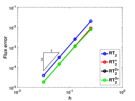
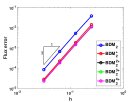
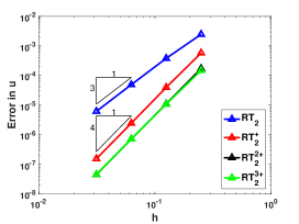
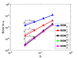
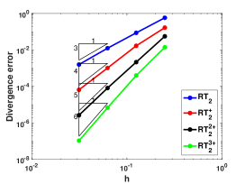
Figure 1: $L^{2}$-errors in the flux (top), in $u$ (middle) and divergence (bottom), using approximation space configurations $RT_{2}^{n+}$ based rectangular meshes (right) and $BDM_{2}^{n+}$ for triangles (left).

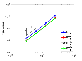
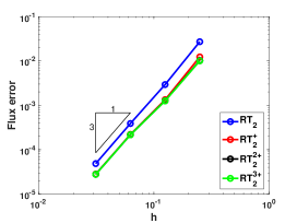
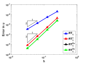
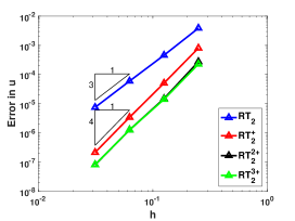
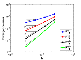
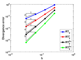
Figure 2: $L^{2}$-errors in the flux (top), in $u$ (middle) and divergence (bottom) with $k=$1 (left) and $k=2$ (right), using trapezoidal meshes and approximation space configurations $RT_{k}^{n+}$, for $n=1,\cdots,3$.

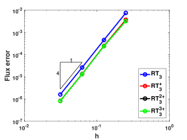
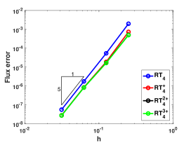
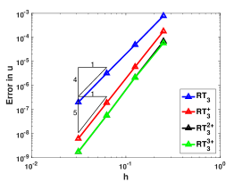
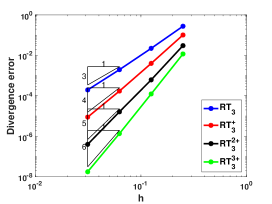
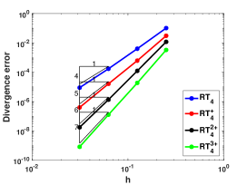
Figure 3: $L^{2}$-errors in the flux (top), in $u$ (middle) and divergence (bottom) with $k=$3 (left) and 4 (right), using trapezoidal meshes and approximation space configurations $RT_{k}^{n+}$, for $n=1,\cdots,3$.

6 Conclusions

A general methodology is developed that is applicable to any space configuration $\hat{\mathbf{V}}_{k},\hat{U}_{k}$, defined in the master element $\hat{K}$, which is supposed to be used for the construction of divergence conforming approximations for vector functions and for their divergence. New insight on approximation properties of the divergence operator in mixed finite elements is obtained by showing that it is possible to enrich the spaces and get discretizations of the divergence operator as accurate as desired, without increasing the size of the condensed linear systems to be solved.

The main requirement is that the original scheme should allow a direct factorization $\hat{\mathbf{V}}_{k}=\hat{\mathbf{V}}^{\partial}_{k}\oplus\mathring{\hat{\mathbf{V}}}_{k}$ of edge and internal flux functions, and that de Rham compatibility formula $\hat{U}_{k}=\nabla\cdot\hat{\mathbf{V}}_{k}$ holds. The enriched versions, which results in higher order convergence rates of the divergence of the flux operator, are defined as $\hat{\mathbf{V}}_{k}^{n+}=\hat{\mathbf{V}}^{\partial}_{k}\oplus\mathring{\hat{\mathbf{V}}}_{k+n}$, with corresponding scalar spaces $\hat{U}_{k}^{n+}=\hat{U}_{k+n}$. Projections allowing to demonstrate the commuting property of the de Rham diagram can be extended to the enriched context. From the coding point of view, the main requirement is that the polynomial order of the edge flux functions can be chosen independently from the polynomial order of the internal flux space. The enriched space $\hat{\mathbf{V}}_{k}^{n+}$ is simply obtained by pruning from $\hat{\mathbf{V}}_{k+n}$ the edge functions of degree $>k$. For applications to mixed formulations, the computational cost of matrix assembly increases with $n$, but the global condensed systems to be solved have same dimension and structure of the original scheme.

References

References

• [1] D.N. Arnold, D. Boffi, and R.S. Falk, Approximation by quadrilateral finite elements, Math. Comp., 71 (2002), pp. 909–922.
• [2] D.N. Arnold, D. Boffi, and R.S. Falk, Quadrilateral H(div) finite elements, SIAM J. Numer. Anal. 42 (6): 2429-2451, 2005.
• [3] F. Brezzi, J. Douglas, M. Fortin, L.D. Marini, Efficient rectangular mixed finite elements in two and three space variable, RAIRO ModΓ©l, Math. Anal. NumΓ©r. 2: 581-604, 1987.
• [4] F. Brezzi, J. Douglas and L.D. Marini, Two Families of Mixed Finite Elements for Second Order Elliptic Problems, Numer. Math. 47: 217-235, 1985.
• [5] F. Brezzi, M. Fortin. 1991. Mixed and Hybrid Finite Element Methods, Springer Series in Computational Mathematics, vol. 15, Springer-Verlag, New York.
• [6] D.A. Castro, P.R.B. Devloo, A.M. Farias, S.M. Gomes, O. DurΓ‘n, Hierarchical high order finite element bases for $\mathbf{H}(\text{div})$ spaces based on curved meshes for two-dimensional regions or manifolds, J. Comput. Appl. Math. 301: 241–258, 2016.
• [7] D. A. Castro, P. R. B. Devloo, A. M. Farias, S. M. Gomes, D. Siqueira, O. DurΓ‘n. Three dimensional hierarchical mixed finite element approximations with enhanced primal variable accuracy. Comput. Methods Appl. Mech. and Engrg. 306 (2016), 479–502.
• [8] B. Cockburn, J. Gopalakrishnan, Error analysis of variable degree mixed methods for elliptic problems via hybridization. Mathematics of Computation 74 (252) (2005), 1653-1677.
• [9] L. Demkowicz, P. Monk, L.Vardapetvan, W. Rachowicz. De Rham diagram for $hp$ finite element spaces. Comput. Math. Appl., 39 (2000), 29-38.
• [10] A.M. Farias, P.R.B. Devloo, S.M. Gomes, D. de Siqueira, D. A. Castro, Two dimensional mixed finite element approximations for elliptic problems with enhanced accuracy for the potential and flux divergence. Comput. Math. Appl. 74: 3283–3295, 2017.
• [11] http://github.com/labmec/neopz
• [12] P.A. Raviart and J.M. Thomas, A mixed finite element method for 2nd order elliptic problems. Lect. Not. Math. 606: 292-315, 1997.
• [13] D. Siqueira, P.R.B. Devloo, S.M. Gomes. A new procedure for the construction of hierarchical high order Hdiv and Hcurl finite element spaces, Journal of Computational and Applied Mathematics, 240: 204-214, 2013.