Ensemble Kalman Inversion: A Derivative-Free Technique For Machine Learning Tasks

Abstract

The standard probabilistic perspective on machine learning gives rise to empirical risk-minimization tasks that are frequently solved by stochastic gradient descent (SGD) and variants thereof. We present a formulation of these tasks as classical inverse or filtering problems and, furthermore, we propose an efficient, gradient-free algorithm for finding a solution to these problems using ensemble Kalman inversion (EKI). Applications of our approach include offline and online supervised learning with deep neural networks, as well as graph-based semi-supervised learning. The essence of the EKI procedure is an ensemble based approximate gradient descent in which derivatives are replaced by differences from within the ensemble. We suggest several modifications to the basic method, derived from empirically successful heuristics developed in the context of SGD. Numerical results demonstrate wide applicability and robustness of the proposed algorithm.

Keywords: Machine learning, Deep learning, Derivative-free optimization, Ensemble Kalman inversion, Ensemble Kalman filtering.

1 Introduction

1.1 The Setting

The field of machine learning has seen enormous advances over the last decade. These advances have been driven by two key elements: (i) the introduction of flexible architectures which have the expressive power needed to efficiently represent the input-output maps encountered in practice; (ii) the development of smart optimization tools which train the free parameters in these input-output maps to match data. The text [21] overviews the start-of-the-art.

While there is little work in the field of derivative-free, paralellizable methods for machine learning tasks, such advancements are greatly needed. Variants on the Robbins-Monro algorithm [63], such as stochastic gradient descent (SGD), have become state-of-the-art for practitioners in machine learning [21] and an attendant theory [14, 3, 70, 48, 37] is emerging. However the approach faces many challenges and limitations [20, 60, 78]. New directions are needed to overcome them, especially for parallelization, as attempts to parallelize SGD have seen limited success [87].

A step in the direction of a derivative-free, parallelizable algorithm for the training of neural networks was attempted in [11] by use of the the method of auxiliary coordinates (MAC). Another approach using the alternating direction method of multipliers (ADMM) and a Bregman iteration is attempted in [78]. Both methods seem successful but are only demonstrated on supervised learning tasks with shallow, dense neural networks that have relatively few parameters. In reinforcement learning, genetic algorithm have seen some success (see [73] and references therein), but it is not clear how to deploy them outside of that domain.

To simultaneously address the issues of parallelizable and derivative-free optimization, we demonstrate in this paper the potential for using ensemble Kalman methods to undertake machine learning tasks. Optimizing neural networks via Kalman filtering has been attempted before (see [26] and references therein), but most have been through the use of Extended or Unscented Kalman Filters. Such methods are plagued by inescapable computational and memory constraints and hence their application has been restricted to small parameter models. A contemporaneous paper by Haber et al [25] has introduced a variant on the ensemble Kalman filter, and applied it to the training of neural networks; our paper works with a more standard implementations of ensemble Kalman methods for filtering and inversion [44, 35] and demonstrates potential for these methods within a wide range of machine learning tasks.

1.2 Our Contribution

The goal of this work is two-fold:

• First we show that many of the common tasks considered in machine learning can be formulated in the unified framework of Bayesian inverse problems. The advantage of this point of view is that it allows for the transfer of theory and algorithms developed for inverse problems to the field of machine learning, in a manner accessible to the inverse problems community. To this end we give a precise, mathematical description of the most common approximation architecture in machine learning, the neural network (and its variants); we use the language of dynamical systems, and avoid references to the neurobiological language and notation more common-place in the applied machine learning literature.

• Secondly, adopting the inverse problem point of view, we show that variants of ensemble Kalman methods (EKI, EnKF) can be just as effective at solving most machine learning tasks as the plethora of gradient-based methods that are widespread in the field. We borrow some ideas from machine learning and optimization to modify these ensemble methods, to enhance their performance.

Our belief is that by formulating machine learning tasks as inverse problems, and by demonstrating the potential for methodologies to be transferred from the field of inverse problems to machine learning, we will open up new ways of thinking about machine learning which may ultimately lead to deeper understanding of the optimization tasks at the heart of the field, and to improved methodology for addressing those tasks. To substantiate the second assertion we give examples of the competitive application of ensemble methods to supervised, semi-supervised, and online learning problems with deep dense, convolutional, and recurrent neural networks. To the best of our knowledge, this is the first paper to successfully apply ensemble Kalman methods to such a range of relatively large scale machine learning tasks. Whilst we do not attempt parallelization, ensemble methods are easily parallelizable and we give references to relevant literature. Our work leaves many open questions and future research directions for the inverse problems community.

1.3 Notation and Overview

We adopt the notation $\mathbb{R}$ for the real axis, $\mathbb{R}_{+}$ the subset of non-negative reals, and $\mathbb{N}=\{0,1,2,\dots\}$ for the set of natural numbers. For any set $A$, we use $A^{n}$ to denote its $n$-fold Cartesian product for any $n\in\mathbb{N}\setminus\{0\}$. For any function $f:A\rightarrow B$, we use $\text{Im}(f)=\{y\in B:y=f(x),{\rm for}\,{\rm some}\,x\in A\}$ to denote its image. For any subset $V\subseteq\mathcal{X}$ of a linear space $\mathcal{X}$, we let $\dim V$ denote the dimension of the smallest subspace containing $V$. For any Hilbert space $\mathcal{H}$, we adopt the notation $\|\cdot\|_{\mathcal{H}}$ and $\langle\cdot,\cdot\rangle_{\mathcal{H}}$ to be its associated norm and inner-product respectively. Furthermore for any symmetric, positive-definite operator $C:\mathcal{D}(C)\subset\mathcal{H}\rightarrow\mathcal{H}$, we use the notation $\|\cdot\|_{C}=\|C^{-\frac{1}{2}}\cdot\|_{\mathcal{H}}$ and $\langle\cdot,\cdot\rangle_{C}=\langle C^{-\frac{1}{2}}\cdot,C^{-\frac{1}{2}}\cdot,\rangle_{\mathcal{H}}$. For any two topological spaces $\mathcal{X},\mathcal{Y}$, we let $C(\mathcal{X},\mathcal{Y})$ denote the set of continuous functions from $\mathcal{X}$ to $\mathcal{Y}$. We define

$$\mathbb{P}^{m}=\{y\in\mathbb{R}^{m}\;|\;\|y\|_{1}=1,y_{1},\dots,y_{m}\geq 0\}$$

the set of $m$-dimensional probability vectors, and the subset

$$\mathbb{P}^{m}_{0}=\{y\in\mathbb{R}^{m}\;|\;\|y\|_{1}=1,y_{1},\dots,y_{m}>0\}.$$

Section 2 delineates the learning problem, starting from the classical, optimization-based framework, and shows how it can be formulated as a Bayesian inverse problem. Section 3 gives a brief overview of modern neural network architectures as dynamical systems. Section 4 outlines the state-of-the-art algorithms for fitting neural network models, as well as the EKI method and our proposed modifications of it. Section 5 presents our numerical experiments, comparing and contrasting EKI methods with the state-of-the-art. Section 6 gives some concluding remarks and possible future directions for this line of work.

2 Problem Formulation

Subsection 2.1 overviews the standard formulation of machine learning problems with subsections 2.1.1, 2.1.2, and 2.1.3 presenting supervised, semi-supervised, and online learning respectively. Subsection 2.2 sets forth the Bayesian inverse problem interpretation of these tasks and gives examples for each of the previously presented problems.

2.1 Classical Framework

The problem of learning is usually formulated as minimizing an expected cost over some space of mappings relating the data [21, 81, 53]. More precisely, let $\mathcal{X}$, $\mathcal{Y}$ be separable Hilbert spaces and let $\mathbb{P}(x,y)$ be a probability measure on the product space $\mathcal{X}\times\mathcal{Y}$. Let $\mathcal{L}:\mathcal{Y}\times\mathcal{Y}\rightarrow\mathbb{R}_{+}$ be a positive-definite function and define $\mathcal{F}$ to be the set of mappings $\{\mathcal{G}:\mathcal{X}\rightarrow\mathcal{Y}\}$ on which the composition $\mathcal{L}(\mathcal{G}(\cdot),\cdot)$ is $\mathbb{P}$-measurable for all $\mathcal{G}$ in $\mathcal{F}$. Then we seek to minimize the functional

$$Q(\mathcal{G})=\int_{\mathcal{X}\times\mathcal{Y}}\mathcal{L}(\mathcal{G}(x),y)\;d\mathbb{P}(x,y).$$ (1)

across all mappings in $\mathcal{F}$. This minimization may not be well defined as there could be infimizing sequences not converging in $\mathcal{F}$. Thus further constraints (regularization) are needed to obtain an unambiguous optimization problem. These are generally introduced by working with parametric forms of $\mathcal{G}$. Additional, explicit regularization is also often added to parameterized versions of (1).

Usually $\mathcal{L}$ is called the loss or cost function and acts as a metric-like function on $\mathcal{Y}$; however it is useful in applications to relax the strict properties of a metric, and we, in particular, do not require $\mathcal{L}$ to be symmetric or subadditive. With this interpretation of $\mathcal{L}$ as a cost, we are seeking a mapping $\mathcal{G}$ with lowest cost, on average with respect to $\mathbb{P}$. There are numerous choices for $\mathcal{L}$ used in applications [21]; some of the most common include the squared-error loss $\mathcal{L}(y^{\prime},y)=\|y-y^{\prime}\|^{2}_{\mathcal{Y}}$ used for regression tasks, and the cross-entropy loss $\mathcal{L}(y^{\prime},y)=-\langle y,\log y^{\prime}\rangle_{\mathcal{Y}}$ used for classification tasks. In both these cases we often have $\mathcal{Y}=\mathbb{R}^{K}$, and, for classification, we may restrict the class of mappings to those taking values in $\mathbb{P}^{K}$.

Most of our focus will be on parametric learning where we approximate $\mathcal{F}$ by a parametric family of models $\{\mathcal{G}(u|\cdot):\mathcal{X}\rightarrow\mathcal{Y}\}$ where $u\in\mathcal{U}$ is the parameter and $\mathcal{U}$ is a separable Hilbert space. This allows us to work with a computable class of functions and perform the minimization directly over $\mathcal{U}$. Much of the early work in machine learning focuses on model classes which make the associated minimization problem convex [9, 31, 53], but the recent empirical success of neural networks has driven research away from this direction [45, 21]. In Section 3, we give a brief overview of the model space of neural networks.

While the formulation presented in (1) is very general, it is not directly transferable to practical applications as, typically, we have no direct access to $\mathbb{P}(x,y)$. How we choose to address this issue depends on the information known to us, usually in the form of a data set, and defines the type of learning. Typically information about $\mathbb{P}$ is accessible only through our sample data. The next three subsections describe particular structures of such sample data sets which arise in applications, and the minimization tasks which are constructed from them to determine the parameter $u$.

2.1.1 Supervised Learning

Suppose that we have a dataset $\{(x_{j},y_{j})\}_{j=1}^{N}$ assumed to be i.i.d. samples from $\mathbb{P}(x,y)$. We can thus replace the integral (1) with its Monte Carlo approximation, and add a regularization term, to obtain the following minimization problem:

$$\mathop{\mathrm{arg\,min}}_{u\in\mathcal{U}}\Phi_{\text{s}}(u;\mathsf{x},\mathsf{y}),$$ (2)

$$\Phi_{\text{s}}(u;\mathsf{x},\mathsf{y})=\frac{1}{N}\sum_{j=1}^{N}\mathcal{L}(\mathcal{G}(u|x_{j}),y_{j})+R(u).$$ (3)

Here $R:\mathcal{U}\rightarrow\mathbb{R}$ is a regularizer on the parameters designed to prevent overfitting or address possible ill-posedness. We use the notation $\mathsf{x}=[x_{1},\dots,x_{N}]\in\mathcal{X}^{N}$, and analogously $\mathsf{y}$, for concatenation of the data in the input and output spaces $\mathcal{X},\mathcal{Y}$ respectively.

A common choice of regularizer is $R(u)=\lambda\|u\|_{\mathcal{U}}^{2}$ where $\lambda\in\mathbb{R}$ is a tunable parameter. This choice is often called weight decay in the machine learning literature. Other choices, such as sparsity promoting norms, are also employed; carefully selected choices of the norm can induce desired behavior in the parameters [10, 82]. We note also that Monte Carlo approximation is itself a form of regularization of the minimization task (1).

This formulation is known as supervised learning. Supervised learning is perhaps the most common type of machine learning with numerous applications including image/video classification, object detection, and natural language processing [43, 50, 76].

2.1.2 Semi-Supervised Learning

Suppose now that we only observe a small portion of the data $\mathsf{y}$ in the image space; specifically we assume that we have access to data $\{x_{j}\}_{j\in Z}$, $\{y_{j}\}_{j\in Z^{\prime}}$ where $x_{j}\in\mathcal{X},y_{j}\in\mathcal{Y}$, $Z=\{1,\dots,N\}$ and where $Z^{\prime}\subset Z$ with $|Z^{\prime}|\ll|Z|$. Clearly this can be turned into supervised learning by ignoring all data indexed by $Z\setminus Z^{\prime}$, but we would like to take advantage of all the information known to us. Often the data in $\mathcal{X}$ is known as unlabeled data, and the data in $\mathcal{Y}$ as labeled data; in particular the labeled data is often in the form of categories. We use the terms labeled and unlabeled in general, regardless or whether the data in $\mathcal{Y}$ is categorical; however some of our illustrative discussion below will focus on the binary classification problem. The objective is to assign a label $y_{j}$ to every $j\in Z$. This problem is known as semi-supervised learning.

One approach to the problem is to seek to minimize

$$\mathop{\mathrm{arg\,min}}_{u\in\mathcal{U}}\Phi_{\text{ss}}(u;\mathsf{x},\mathsf{y})$$ (4)

$$\Phi_{\text{ss}}(u;\mathsf{x},\mathsf{y})=\frac{1}{|Z^{\prime}|}\sum_{j\in Z^{\prime}}\mathcal{L}(\mathcal{G}(u|x_{j}),y_{j})+R(u;\mathsf{x})$$ (5)

where the regularizer $R(u;\mathsf{x})$ may use the unlabeled data in $Z\backslash Z^{\prime}$, but the loss term involves only labeled data in $Z^{\prime}$.

There are a variety of ways in which one can construct the regularizer $R(u;\mathsf{x})$ including graph-based and low-density separation methods [7, 6]. In this work, we will study a nonparametric graph approach where we think of $Z$ as indexing the nodes on a graph. To illustrate ideas we consider the case of binary outputs, take $\mathcal{Y}=\mathbb{R}$ and restrict attention to mappings $\mathcal{G}(u|\cdot)$ which take values in $\{-1,1\}$; we sometimes abuse notation and simply take $\mathcal{Y}=\{-1,1\}$, so that $\mathcal{Y}$ is no longer a Hilbert space. We assume that $\mathcal{U}$ comprises real-valued functions on the nodes $Z$ of the graph, equivalently vectors in $\mathbb{R}^{N}$. We specify that $\mathcal{G}(u|j)=\text{sgn}(u(j))$ for all $j\in Z$, and take, for example, the probit or logistic loss function [62, 7]. Once we have found an optimal parameter value for $u:Z\rightarrow\mathbb{R}$, application of $\mathcal{G}$ to $u$ will return a labeling over all nodes $j$ in $Z$. In order to use all the unlabeled data we introduce edge weights which measure affinities between nodes of a graph with vertices $Z$, by means of a weight function on $\mathcal{X}\times\mathcal{X}$. We then compute the graph Laplacian $\mathsf{L}(\mathsf{x})$ and use it to define a regularizer in the form

$$R(u;\mathsf{x})=\langle u,(\mathsf{L}(\mathsf{x})+\tau^{2}I)^{\alpha}u\rangle_{\mathbb{R}^{N}}.$$

Here $I$ is the identity operator, and $\tau,\alpha\in\mathbb{R}$ with $\alpha>0$ are tunable parameters. Further details of this method are in the following section. Applications of semi-supervised learning can include any situation where data in the image space $\mathcal{Y}$ is hard to come by, for example because it requires expert human labeling; a specific example is medical imaging [49].

2.1.3 Online Learning

Our third and final class of learning problems concerns situations where samples of data are presented to us sequentially and we aim to refine our choice of parameters at each step. We thus have the supervised learning problem (2) and we aim to solve it sequentially as each pair of data points $\{x_{j},y_{j}\}$ is delivered. To facilitate cheap algorithms we impose a Markovian structure in which we are allowed to use only the current data sample, as well as our previous estimate of the parameters, when searching for the new estimate. We look for a sequence $\{u_{j}\}_{j=1}^{\infty}\subset\mathcal{U}$ such that $u_{j}\rightarrow u^{*}$ as $j\rightarrow\infty$ where, in the perfect scenario, $u^{*}$ will be a minimizer of the limiting learning problem (1). To make the problem Markovian, we may formulate it as the following minimization task

$$u_{j}=\mathop{\mathrm{arg\,min}}_{u\in\mathcal{U}}\Phi_{\text{o}}(u,u_{j-1};x_{j},y_{j})$$ (6)

$$\Phi_{\text{o}}(u,u_{j-1};x_{j},y_{j})=\mathcal{L}(\mathcal{G}(u|x_{j}),y_{j})+R(u;u_{j-1})$$ (7)

where $R$ is again a regularizer that could enforce a closeness condition between consecutive parameter estimates, such as

$$R(u;u_{j-1})=\lambda\|u-u_{j-1}\|^{2}_{\mathcal{U}}.$$

Furthermore this regularization need not be this explicit, but could rather be included in the method chosen to solve (6). For example if we use an iterative method for the minimization, we could simply start the iteration at $u_{j-1}$.

This formulation of supervised learning is known as online learning. It can be viewed as reducing computational cost as a cheaper, sequential way of estimating a solution to (1); or it may be necessitated by the sequential manner in which data is acquired.

2.2 Inverse Problems

The preceding discussion demonstrates that, while the goal of learning is to find a mapping which generalizes across the whole distribution of possible data, in practice, we are severely restricted by only having access to a finite data set. Namely formulations (2), (4), (6) can be stated for any input-output pair data set with no reference to $\mathbb{P}(x,y)$ by simply assuming that there exists some function in our model class that will relate the two. In fact, since $\mathcal{L}$ is positive-definite, its dependence also washes out when ones takes a function approximation point of view. To make this precise, consider the inverse problem of finding $u\in\mathcal{U}$ such that

$$\mathsf{y}=\mathsf{G}(u|\mathsf{x})+\eta;$$ (8)

here $\mathsf{G}(u|\mathsf{x})=[\mathcal{G}(u|x_{1}),\dots,\mathcal{G}(u|x_{N})]$ is a concatenation and $\eta\sim\pi$ is a $\mathcal{Y}^{N}$-valued random variable distributed according to a measure $\pi$ that models possible noise in the data, or model error. In order to facilitate a Bayesian formulation of this inverse problem we let $\mu_{0}$ denote a prior probability measure on the parameters $u$. Then supposing

$$-\log(\pi(\mathsf{y}-\mathsf{G}(u|\mathsf{x}))) \propto\sum_{j=1}^{N}\mathcal{L}(\mathcal{G}(u|x_{j}),y_{j})$$

$$-\log(\mu_{0}(u)) \propto R(u)$$

we see that (2) corresponds to the standard MAP estimator arising from a Bayesian formulation of (8). The semi-supervised learning problem (4) can also be viewed as a MAP estimator by restricting (8) to $Z^{\prime}$ and using $\mathsf{x}$ to build $\mu_{0}$. This is the perspective we take in this work and we illustrate with an example for each type of problem.

Example 2.1.

Suppose that $\mathcal{Y}$ and $\mathcal{U}$ are Euclidean spaces and let $\pi=\mathcal{N}(0,\Gamma)$ and $\mu_{0}=\mathcal{N}(0,\Sigma)$ be Gaussian with positive-definite covariances $\Gamma,\Sigma$ where $\Gamma$ is block-diagonal with $N$ identical blocks $\Gamma_{0}$. Computing the MAP estimator of (8), we obtain that $\mathcal{L}(y^{\prime},y)=\|y-y^{\prime}\|_{\Gamma_{0}}^{2}$ and $R(u)=\|u\|_{\Sigma}^{2}$.

Example 2.2.

Suppose that $\mathcal{U}=\mathbb{R}^{N}$ and $\mathcal{Y}=\mathbb{R}$ with the data $y_{j}=\pm 1$ $\forall j\in Z^{\prime}$. We will take the model class to be a single function $\mathcal{G}:\mathbb{R}^{N}\times Z\rightarrow\mathbb{R}$ depending only on the index of each data point and defined by $\mathcal{G}(u|j)=\text{sgn}(u_{j})$. As mentioned, we think of $Z$ as the nodes on a graph and construct the edge set $E=(e_{ij})=\eta(x_{i},x_{j})$ where $\eta:\mathcal{X}\times\mathcal{X}\rightarrow\mathbb{R}_{+}$ is a symmetric function. This allows construction of the associated graph Laplacian $\mathsf{L}(\mathsf{x})$. We shift it and remove its null space and consider the symmetric, positive-definite operator $C=(\mathsf{L}(\mathsf{x})+\tau^{2}I)^{-\alpha}$ from which we can define the Gaussian measure $\mu_{0}=\mathcal{N}(0,C)$. For details on why this construction defines a reasonable prior we refer to [7]. Letting $\pi=\mathcal{N}(0,\frac{1}{\gamma^{2}}I)$, we restrict (8) to the inverse problem

$$y_{j}=\mathcal{G}(u|j)+\eta_{j}\quad\forall j\in Z^{\prime}.$$

With the given definitions, letting $\gamma^{2}=|Z^{\prime}|$, the associated MAP estimator has the form of (4), namely

$$\frac{1}{|Z^{\prime}|}\sum_{j\in Z^{\prime}}|\mathcal{G}(u|j)-y_{j}|^{2}+\langle u,C^{-1}u\rangle_{\mathbb{R}^{N}}.$$

The infimum for this functional is not achieved [34], but the ensemble based methods we employ to solve the problem implicitly apply a further regularization which circumvents this issue.

Example 2.3.

Lastly we turn to the online learning problem (6). We assume that there is some unobserved, fixed in time parameter of our model that will perfectly match the observed data up to a noise term. Our goal is to estimate this parameter sequentially. Namely, we consider the stochastic dynamical system,

$$\begin{split}u_{j+1}&=u_{j}\\ y_{j+1}&=\mathcal{G}(u_{j+1}|x_{j+1})+\eta_{j+1}\end{split}$$ (9)

where the sequence $\{\eta_{j}\}$ are $\mathcal{Y}$-valued i.i.d. random variables that are also independent from the data. This is an instance of the classic filtering problem considered in data assimilation [44]. We may view this as solving an inverse problem at each fixed time with increasingly strong prior information as time unrolls. With the appropriate assumptions on the prior and the noise model, we may again view (6) as the MAP estimators of each fixed inverse problem. Thus we may consider all problems presented here in the general framework of (8).

3 Approximation Architectures

In this section, we outline the approximation architectures that we will use to solve the three machine learning tasks outlined in the preceding section. For supervised and online learning these amount to specifying the dependence of $\mathcal{G}$ on $u$; for semi-supervised learning this corresponds to determining a basis in which to seek the parameter $u$. We do not give further details for the semi-supervised case as our numerics fit in the context of Example 2.2, but we refer the reader to [7] for a detailed discussion.

Subsection 3.1 details feed-forward neural networks with subsections 3.1.1 and 3.1.2 showing the parameterizations of dense and convolutional networks respectively. Subsection 3.2 presents basic recurrent neural networks.

3.1 Feed-Forward Neural Networks

Feed-forward neural networks are a parametric model class defined as discrete time, nonautonomous, semi-dynamical systems of an unusual type. Each map in the composition takes a specific parametrization and can change the dimension of its input while the whole system is computed only up to a fixed time horizon. To make this precise, we will assume $\mathcal{X}=\mathbb{R}^{d}$, $\mathcal{Y}=\mathbb{R}^{m}$ and define a neural network with $n\in\mathbb{N}$ hidden layers as the composition

$$\mathcal{G}(u|x)=S\circ A\circ F_{n-1}\circ\dots\circ F_{0}\circ x$$

where $d_{0}=d$ and $F_{j}\in C(\mathbb{R}^{d_{j}},\mathbb{R}^{d_{j+1}}),n=0,\dots,n-1$ are nonlinear maps, referred to as layers, depending on parameters $\theta_{0},\dots,\theta_{n-1}$ respectively, $A:\mathbb{R}^{d_{n}}\rightarrow\mathbb{R}^{m}$ is an affine map with parameters $\theta_{n}$, and $u=[\theta_{0},\dots,\theta_{n}]$ is a concatenation. The map $S:\mathbb{R}^{m}\rightarrow V\subseteq\mathbb{R}^{m}$ is fixed and thought of as a projection or thresholding done to move the output to the appropriate subset of data space. The choice of $S$ is dependent on the problem at hand. If we are considering a regression task and $V=\mathbb{R}^{m}$ then $S$ can simply be taken as the identity. On the other hand, if we are considering a classification task and $V=\mathbb{P}^{m}$, the set of probability vectors in $\mathbb{R}^{m}$, then $S$ is often taken to be the softmax function defined as

$$S(w)=\frac{1}{\sum_{j=1}^{m}e^{w_{j}}}(e^{w_{1}},\dots,e^{w_{m}}).$$

From this perspective, the neural network approximates a categorical distribution of the input data and the softmax arises naturally as the canonical response function of the categorical distribution (when viewed as belonging to the exponential family of distributions) [51, 65]. If we have some specific bounds for the output data, for example $V=[-1,1]^{m}$ then $S$ can be a point-wise hyperbolic tangent.

What makes this dynamic unusual is the fact that each map can change the dimension of its input unlike a standard dynamical system which operates on a fixed metric space. However, note that the sequence of dimension changes $d_{1},\dots,d_{n}$ is simply a modeling choice that we may alter. Thus let $d_{\max}=\max\{d_{0},\dots,d_{n}\}$ and consider the solution map $\phi:\mathbb{N}_{0}\times\mathbb{N}_{0}\times\mathbb{R}^{d_{\max}}\rightarrow\mathbb{R}^{d_{\max}}$ generated by the nonautonomous difference equation

$$z_{k+1}=F_{k}(z_{k})$$

where each map $F_{k}\in C(\mathbb{R}^{d_{\max}},\mathbb{R}^{d_{\max}})$ is such that $\dim\text{Im}(F_{k})\leq d_{k+1}$; then $\phi(n,m,x)$ is $z_{n}$ given that $z_{m}=x$. We may then define a neural network as

$$\mathcal{G}(u|x)=S\circ A\circ\phi(n,0,\mathcal{P}x)$$

where $\mathcal{P}:\mathbb{R}^{d}\rightarrow\mathbb{R}^{d_{\max}}$ is a projection operator and $A:\mathbb{R}^{d_{\text{max}}}\rightarrow\mathbb{R}^{m}$ is again an affine map. While this definition is mathematically satisfying and potentially useful for theoretical analysis as there is a vast literature on nonautonomus semi-dynamical systems [42], in practice, it is more useful to think of each map as changing the dimension of its input. This is because it allows us to work with parameterizations that explicitly enforce the constraint on the dimension of the image. We take this point of view for the rest of this section to illustrate the practical uses of neural networks.

3.1.1 Dense Networks

A key feature of neural networks is the specific parametrization of each map $F_{k}$. In the most basic case, each $F_{k}$ is an affine map followed by a point-wise nonlinearity, in particular,

$$F_{k}(z_{k})=\sigma(W_{k}z_{k}+b_{k})$$

where $W_{k}\in\mathbb{R}^{d_{k+1}\times d_{k}}$, $b_{k}\in\mathbb{R}^{d_{k+1}}$ are the parameters i.e. $\theta_{k}=[W_{k},b_{k}]$ and $\sigma\in C(\mathbb{R},\mathbb{R})$ is non-constant, bounded, and monotonically increasing; we extend $\sigma$ to a function on $\mathbb{R}^{d}$ by defining it point-wise as $\sigma(u)_{j}=\sigma(u_{j})$ for any vector $u\in\mathbb{R}^{d}$. This layer type is referred to as dense, or fully-connected, because each entry in $W_{k}$ is a parameter with no global sparsity assumptions and hence we can end up with a dense matrix. A neural network with only this type of layer is called dense or fully-connected (DNN).

The nonlinearity $\sigma$, called the activation function, is a design choice and usually does not vary from layer to layer. Some popular choices include the sigmoid, the hyperbolic tangent, or the rectified linear unit (ReLU) defined by $\sigma(q)=\max\{0,q\}$. Note that ReLU is unbounded and hence does not satisfy the assumptions for the classical universal approximation theorem [32], but it has shown tremendous numerical success when the associated inverse problem is solved via backpropagation (method of adjoints) [55].

3.1.2 Convolutional Networks

Instead of seeking the full representation of a linear operator at each time step, we may consider looking only for the parameters associated to a pre-specified type of operator. Namely we consider

$$F_{k}(z_{k})=\sigma(W(s_{k})z_{k}+b_{k})$$

where $W$ can be fully specified by the parameter $s_{k}$. The most commonly considered operator is the one arising from a discrete convolution [46]. We consider the input $z_{k}$ as a function on the integers with period $d_{k}$ then we may define $W(s_{k})$ as the circulant matrix arising as the kernel of the discrete circular convolution with convolution operator $s_{k}$. Exact construction of the operator $W$ is a modeling choice as one can pick exactly which blocks of $z_{k}$ to compute the convolution over. Usually, even with maximally overlapping blocks, the operation is dimension reducing, but can be made dimension preserving, or even expanding, by appending zero entries to $z_{k}$. This is called padding. For brevity, we omit exact descriptions of such details and refer the reader to [21]. The parameter $s_{k}$ is known as the stencil. Neural networks following this construction are called convolutional (CNN).

In practice, a CNN computes a linear combination of many convolutions at each time step, namely

$$F_{k}^{(j)}(z_{k})=\sigma\left(\sum_{m=1}^{M_{k}}W(s_{k}^{(j,m)})z_{k}^{(m)}+b_{k}^{(j)}\right)$$

for $j=1,2,\dots,M_{k+1}$ where $z_{k}=[z_{k}^{(1)},\dots,z_{k}^{(M_{k})}]$ with each entry known as a channel and $M_{k}=1$ if no convolutions were computed at the previous iteration. Finally we define $F_{k}(z_{k})=[F_{k}^{(1)}(z_{k}),\dots,F_{k}^{(M_{k+1})}(z_{k})]$. The number of channels at each time step, the integer $M_{k+1}$, is a design choice which, along with the choice for the size of the stencils $s_{k}^{(j,m)}$, the dimension of the input, and the design of $W$ determine the dimension of the image space $d_{k+1}$ for the map $F_{k}$.

When employing convolutions, it is standard practice to sometimes place maps which compute certain statistics from the convolution. These operations are commonly referred to as pooling [54]. Perhaps the most common such operation is known as max-pooling. To illustrate suppose $[F^{(1)}_{k},\dots,F^{(M_{k+1})}_{k}]$ are the $M_{k+1}$ channels computed as the output of a convolution (dropping the $z_{k}$ dependence for notational convenience). In this context, it is helpful to change perspective slightly and view each $F^{(j)}_{k}$ as a matrix whose concatenation gives the vector $F_{k}$. Each of these matrices is a two-dimensional grid whose value at each point represents a linear combination of convolutions each computed at that spatial location. We define a maximum-based, block-subsampling operation

$$(p^{(j)}_{k})_{il}=\max_{q\in\{1,\dots,H_{1}\}}\max_{v\in\{1,\dots,H_{2}\}}(F^{(j)}_{k})_{\alpha(i-1)+q,\beta(l-1)+v}$$

where the tuple $(H_{1},H_{2})\in\mathbb{N}^{2}$ is called the pooling kernel and the tuple $(\alpha,\beta)\in\mathbb{N}^{2}$ is called the stride, each a design choice for the operation. It is common practice to take $H_{1}=H_{2}=\alpha=\beta$. We then define the full layer as $F_{k}(z_{k})=[p^{(1)}_{k}(z_{k}),\dots,p^{(M_{k+1})}_{k}(z_{k})]$. There are other standard choices for pooling operations including average pooling, $\ell_{p}$-pooling, fractional max-pooling, and adaptive max-pooling where each of the respective names are suggestive of the operation being performed; details may be found in [79, 23, 24, 27]. Note that pooling operations are dimension reducing and are usually thought of as a way of extracting the most important information from a convolution. When one chooses the kernel $(H_{1},H_{2})$ such that $F^{(j)}_{k}\in\mathbb{R}^{H_{1}\times H_{2}}$, the per channel output of the pooling is a scalar and the operation is called global pooling.

Convolutional Neural Network
Map	Type	Notation
$F_{0}:\mathbb{R}^{28\times 28}\rightarrow\mathbb{R}^{32\times 24\times 24}$	Conv 32x5x5	$M_{0}=1,M_{1}=32,s_{0}^{(j,m)}\in\mathbb{R}^{5\times 5}$
		$j\in\{1,\dots,32\},m=\{1\}$
$F_{1}:\mathbb{R}^{32\times 24\times 24}\rightarrow\mathbb{R}^{32\times 10\times 10}$	Conv 32x5x5	$M_{2}=32,s_{1}^{(j,m)}\in\mathbb{R}^{5\times 5}$
	MaxPool 2x2	$j\in\{1,\dots,32\},m\in\{1,\dots,32\}$
		$H_{1}=H_{2}=2$ ($\alpha=\beta=2$)
$F_{2}::\mathbb{R}^{32\times 10\times 10}\rightarrow\mathbb{R}^{64\times 6\times 6}$	Conv 64x5x5	$M_{3}=64,s_{2}^{(j,m)}\in\mathbb{R}^{5\times 5}$
		$j\in\{1,\dots,64\},m\in\{1,\dots,32\}$
$F_{3}:\mathbb{R}^{64\times 6\times 6}\rightarrow\mathbb{R}^{64}$	Conv 64x5x5	$M_{4}=64,s_{3}^{(j,m)}\in\mathbb{R}^{5\times 5}$
	MaxPool 2x2	$j\in\{1,\dots,64\},m\in\{1,\dots,64\}$
	(global)	$H_{1}=H_{2}=2$
$F_{4}:\mathbb{R}^{64}\rightarrow\mathbb{R}^{500}$	FC-500	$W_{4}\in\mathbb{R}^{500\times 64},b_{4}\in\mathbb{R}^{500}$
$A:\mathbb{R}^{500}\rightarrow\mathbb{R}^{10}$	FC-10	$W_{5}\in\mathbb{R}^{10\times 500},b_{5}\in\mathbb{R}^{10}$
$S:\mathbb{R}^{10}\rightarrow\mathbb{R}^{10}$	Softmax	$S(w)=\frac{1}{\sum_{j=1}^{10}e^{w_{j}}}(e^{w_{1}},\dots,e^{w_{10}})$

Figure 1: A four layer convolutional neural network for classifying images in the MNIST data set. The middle column shows a description typical of the machine learning literature. The other two columns connect this jargon to the notation presented here. No padding is added and the convolutions are computed over maximally overlapping blocks (stride of one). The nonlinearity $\sigma$ is the ReLU and is the same for every layer.

Figure 2: Output of each map from left to right of the convolutinal neural network shown in Figure 1. The left most image is the input and the next three images show a single randomly selected channel from the outputs of $F_{0},F_{1},F_{2}$ respectively. The outputs of $F_{3},F_{4},A,S$ are vectors shown respectively in the four subsequent plots. We see that with high probability the network determines that the image belongs to the first class (0) which is correct.

Designs of feed-forward neural networks usually employ both convolutional (with and without pooling) and dense layers. While the success of convolutional networks has mostly come from image classification or object detection tasks [43], they can be useful for any data with spatial correlations [8, 21]. To connect the complex notation presented in this section with the standard in machine learning literature, we will give an example of a deep convolutional neural network. We consider the task of classifying images of hand-written digits given in the MNIST dataset [47]. These are $28\times 28$ grayscale images of which there are $N=60,000$ and 10 overall classes $\{0,\dots,9\}$ hence we consider $\mathcal{X}=\mathbb{R}^{28\times 28}\cong\mathbb{R}^{784}$ and $\mathcal{Y}$ the space of probability vectors over $\mathbb{R}^{10}$. Figure 1 show a typical construction of a deep convolutional neural network for this task. The word deep is generally reserved for models with $n>3$. Once the model has been fit, Figure 2 shows the output of each map on an example image. Starting with the digitized digit $0$, the model computes its important features, through a sequence of operations involving convolutional layers, culminating in the second to last plot, the output of the affine map $A$. This plot shows model determining that the most likely digit is $0$, but also giving substantial probability weight on the digit $6$. This makes sense, as the digits $0$ and $6$ can look quite similar, especially when hand-written. Once the softmax is taken (because it exponentiates), the probability of the image being a $6$ is essentially washed out, as shown in the last plot. This is a short-coming of the softmax as it may not accurately retain the confidence of the model’s prediction. We stipulate that this may be a reason for the emergence of highly-confident adversarial examples [77, 22], but do not pursue suitable modifications in this work.

3.2 Recurrent Neural Networks

Recurrent neural networks are models for time-series data defined as discrete time, nonautonomous, semi-dynamical systems that are parametrized by feed-forward neural networks. To make this precise, we first define a layer of two-inputs simply as the sum of two affine maps followed by a point-wise nonlinearity, namely for $j=1,\dots,n$ define $F_{\theta_{j}}:\mathbb{R}^{d_{h}}\times\mathbb{R}^{d}\rightarrow\mathbb{R}^{d_{h}}$ by

$$F_{\theta_{j}}(z,q)=\sigma(W^{(j)}_{h}z+b^{(j)}_{h}+W^{(j)}_{x}q+b^{(j)}_{x})$$

where $W^{(j)}_{h}\in\mathbb{R}^{d_{h}\times d_{h}}$, $W^{(j)}_{x}\in\mathbb{R}^{d_{h}\times d}$ and $b^{(j)}_{h},b^{(j)}_{x}\in\mathbb{R}^{d_{h}}$; the parameters are then given by the concatenation $\theta_{j}=[W^{(j)}_{h},W^{(j)}_{x},b^{(j)}_{h},b^{(j)}_{x}]$. The dimension $d_{h}$ is a design choice that we can pick on a per-problem basis. Now define the map $F_{\theta}:\mathbb{R}^{d_{h}}\times\mathbb{R}^{d}\rightarrow\mathbb{R}^{d_{h}}$ by composing along the first component

$$F_{\theta}(z,q)=F_{\theta_{n}}(F_{\theta_{n-1}}(\dots F_{\theta_{1}}(z,q),\dots q),q),q)$$

where $\theta=[\theta_{1},\dots,\theta_{n}]$ is a concatenation. Now suppose $x_{0},\dots,x_{T-1}\in\mathbb{R}^{d}$ is an observed time series and define the dynamic

$$h_{t+1}=F_{\theta}(h_{t},x_{t})$$

up to time $t=T$. We can think of this as a nonautonomous, semi-dynamical system on $\mathbb{R}^{d_{h}}$ with parameter $x=[x_{0},\dots,x_{T-1}]$. Let $\phi:\{0,\dots,T\}\times\mathbb{R}^{T\times d}\times\mathbb{R}^{d_{h}}\rightarrow\mathbb{R}^{d_{h}}$ be the solution map generated by this difference equation. We can finally define a recurrent neural network $\mathcal{G}(u|\cdot):\mathbb{R}^{T\times d}\rightarrow V\subseteq\mathbb{R}^{T\times d}$ by

$$\mathcal{G}(u|x)=\begin{bmatrix}S(A_{1}\circ\phi(1,x,h_{0}))\\ S(A_{2}\circ\phi(2,x,h_{0}))\\ \vdots\\ S(A_{T}\circ\phi(T,x,h_{0}))\end{bmatrix}$$

where $A_{1},\dots,A_{T}$ are affine maps, $S$ is a thresholding (such as softmax) as previously discussed, and $u$ a concatenation of the parameters $\theta$ as well as the parameters for all of the affine maps. Usually ones takes $h_{0}=0$, but randomly generated initial conditions are also used in practice.

The construction presented here is the most basic recurrent neural network. Many others architectures such as Long Short-Term Memory (LSTM), recursive, and bi-recurrent networks have been proposed in the literature [69, 30, 29, 21], but they are all slight modifications to the above dynamic. These architectures can be used as sequence to sequence maps, or, if we only consider the output at the last time that is $S(A_{T}\circ\phi(T,x,h_{0}))$, as predicting $x_{T}$ or classifying the sequence $x_{0},\dots,x_{T-1}$. We refer the reader to [74] for an overview of the applications of recurrent neural networks.

4 Algorithms

Subsection 4.1 describes the choice of loss function. Subsection 4.2 outlines the state-of-the-art derivative based optimization, with subsection 4.2.1 presenting the algorithms and subsection 4.2.2 presenting tricks for better convergence. Subsection 4.3 defines the EKI method, with subsequent subsections presenting our various modifications.

4.1 Loss Function

Before delving into the specifics of optimization methods used, we discuss the general choice of loss function $\mathcal{L}$. While the machine learning literature contains a wide variety of loss functions that are designed for specific problems, there are two which are most commonly used and considered first when tackling any regression and classification problems respectively, and on which we focus our work in this paper. For regression tasks, the squared-error loss

$$\mathcal{L}(y^{\prime},y)=\|y-y^{\prime}\|_{\mathcal{Y}}^{2}$$

is standard and is well known to the inverse problems community; it arises from an additive Gaussian noise model. When the task at hand is classification, the standard choice of loss is the cross-entropy

$$\mathcal{L}(y^{\prime},y)=-\langle y,\log y^{\prime}\rangle_{\mathcal{Y}},$$

with the $\log$ computed point-wise and where we consider $\mathcal{Y}=\mathbb{R}^{m}$. This loss is well-defined on the space $\mathbb{P}^{m}_{0}\times\mathbb{P}^{m}$. It is consistent with the the projection map $S$ of the neural network model being the softmax as $\text{Im}(S)=\mathbb{P}^{m}_{0}$. A simple Lagrange multiplier argument shows that $\mathcal{L}$ is indeed infimized over $\mathbb{P}^{m}_{0}$ by sequence $y^{\prime}\rightarrow y$ and hence the loss is consistent with what we want our model output to be. From a modeling perspective, the choice of softmax as the output layer has some drawbacks as it only allows us to asymptotically match the data. However it is a good choice if the cross-entropy loss is used to solve the problem; indeed, in practice, the softmax along with the cross-entropy loss has seen the best numerical results when compared to other choices of thresholding/loss pairs [21].

The interpretation of the cross-entropy loss is to think of our model as approximating a categorical distribution over the input data and, to get this approximation, we want to minimize its Shannon cross-entropy with respect to the data. Note, however, that there is no additive noise model for which this loss appears in the associated MAP estimator simply because $\mathcal{L}$ cannot be written purely as a function of the residual $y-y^{\prime}$.

4.2 Gradient Based Optimization

4.2.1 The Iterative Technique

The current state of the art for solving optimization problems of the form (2), (4), (6) is based around the use of stochastic gradient descent (SGD) [63, 39, 66]. We will describe these methods starting from a continuous time viewpoint, for pedagogical clarity. In particular, we think of the unknown parameter $u\in\mathcal{U}$ as the large time limit of a smooth function of time $u:[0,\infty)\rightarrow\mathcal{U}$. Let $\Phi(u;\mathsf{x},\mathsf{y})=\Phi_{\text{s}}(u;\mathsf{x},\mathsf{y})\text{ or }\Phi_{\text{ss}}(u;\mathsf{x},\mathsf{y})$ then gradient descent imposes the dynamic

$$\dot{u}=-\nabla\Phi(u;\mathsf{x},\mathsf{y}),\quad u(0)=u_{0}$$ (10)

which moves the parameter in the steepest descent direction with respect to the regularized loss function, and hence will converge to a local minimum for Lebesgue almost all initial data, leading to bounded trajectories [48, 71].

For the practical implementations of this approach in machine learning, a number of adaptations are made. First the ODE is discretized in time, typically by a forward Euler scheme; the time-step is referred to as the learning rate. The time-step is often, but not always, chosen to be a decreasing function of the iteration step [14, 63]. Secondly, at each step of the iteration, only a subset of the data is used to approximate the full gradient. In the supervised case, for example,

$$\Phi_{\text{s}}(u;\mathsf{x},\mathsf{y})\approx\frac{1}{N^{\prime}}\sum_{j\in B_{N^{\prime}}}\mathcal{L}(\mathcal{G}(u|x_{j}),y_{j})+R(u)$$

where $B_{N^{\prime}}\subset\{1,\dots,N\}$ is a random subset of cardinality $N^{\prime}$ usually with $N^{\prime}\ll N$. A new $B_{N^{\prime}}$ is drawn at each step of the Euler scheme without replacement until the full dataset has been exhausted. One such cycle through all of the data is called an epoch. The number of epochs it takes to train a model varies significantly based on the model and data at hand but is usually within the range 10 to 500. This idea, called mini-batching, leads to the terminology stochastic gradient descent (SGD). Recent work has suggested that adding this type of noise helps preferentially guide the gradient descent towards places in parameter space which generalize better than standard descent methods [12, 13].

A third variant on basic gradient descent is the use of momentum-augmented methods utilized to accelerate convergence [56]. The continuous time dynamic associated with the Nesterov momentum method is [72]

$$\begin{split}&\ddot{u}+\frac{3}{t}\dot{u}=-\nabla\Phi(u;\mathsf{x},\mathsf{y}),\\ &u(0)=u_{0},\quad\dot{u}(0)=0.\end{split}$$ (11)

We note, however, that, while still calling it Nesterov momentum, this is not the dynamic machine learning practitioners discretize. In fact, what has come to be called Nesterov momentum in the machine learning literature is nothing more than a strange discretization of a rescaled version the standard gradient flow (10). To see this, we note that via the approximation $k/(k+3)\approx 1-3/(k+1)$ one may discretize (11), as is done in [72], to obtain

$$u_{k+1} =v_{k}-h_{k}\nabla\Phi(v_{k};\mathsf{x},\mathsf{y})$$

$$v_{k+1} =u_{k+1}+\frac{k}{k+3}(u_{k+1}-u_{k})$$

with $v_{0}=u_{0}$ and where the sequence $\{\sqrt{h_{k}}\}$ gives the step sizes. However, what machine learning practitioners use is the algorithm

$$u_{k+1} =v_{k}-h_{k}\nabla\Phi(v_{k};\mathsf{x},\mathsf{y})$$

$$v_{k+1} =u_{k+1}+\lambda(u_{k+1}-u_{k})$$

for some fixed $\lambda\in(0,1)$. This may be written as

$$u_{k+1}=(1+\lambda)u_{k}-\lambda u_{k-1}-h_{k}\nabla\Phi((1+\lambda)u_{k}-\lambda u_{k-1};\mathsf{x},\mathsf{y}).$$

If we rearrange and divide by $h_{k}$, we can obtain

$$\frac{u_{k+1}-u_{k}}{h_{k}}=\lambda\left(\frac{u_{k}-u_{k_{1}}}{h_{k}}\right)-\nabla\Phi((1+\lambda)u_{k}-\lambda u_{k-1};\mathsf{x},\mathsf{y})$$

which is easily seen as a discretization of a rescaled version of the gradient flow (10), namely

$$\dot{u}=-(1-\lambda)^{-1}\nabla\Phi(u;\mathsf{x},\mathsf{y}).$$

However, there is a sense in which this discretization introduces momentum, but only to order $\mathcal{O}(h_{k})$ whereas classically the momentum term would be on the order $\mathcal{O}(1)$. To see this, we can again rewrite the discretization as

$$u_{k+1}=2u_{k}-u_{k-1}-(1-\lambda)(u_{k}-u_{k-1})-h_{k}\nabla\Phi((1+\lambda)u_{k}-\lambda u_{k-1};\mathsf{x},\mathsf{y}).$$

Rearranging this and dividing through by $h_{k}$ we can obtain

$$h_{k}\left(\frac{u_{k+1}-2u_{k}+u_{k-1}}{h_{k}^{2}}\right)+(1-\lambda)\left(\frac{u_{k}-u_{k-1}}{h_{k}}\right)=-\nabla\Phi((1+\lambda)u_{k}-\lambda u_{k-1};\mathsf{x},\mathsf{y})$$

which may be seen as a discretization of the equation

$$h_{t}\ddot{u}+(1-\lambda)\dot{u}=-\nabla\Phi(u;\mathsf{x},\mathsf{y}),$$

where $h_{t}$ is a continuous time version of the sequence $\{h_{k}\}$; in particular, if $h_{t}=h\ll 1$ we see that whilst momentum is approximately present, it is only a small effect.

From these variants on continuous time gradient descent have come a plethora of adaptive first-order optimization methods that attempt to solve the learning problem. Some of the more popular include Adam, RMSProp, and Adagrad [40, 15]. There is no consensus on which methods performs best although some recent work has argued in favor of SGD and momentum SGD [85].

Lastly, the online learning problem (6) is also commonly solved via a gradient descent method dubbed online gradient descent (OGD). The dynamic is

$$\dot{u}_{j}=-\nabla\Phi_{\text{o}}(u_{j},u_{j-1};x_{j},y_{j})$$

$$u_{j}(0)=u_{j-1}$$

which can be extended to the momentum case in the obvious way. It is common that only a single step of the Euler scheme is computed. The process of letting all these ODE(s) evolve in time is called training.

4.2.2 Initialization and Normalization

Two major challenges for the iterative methods presented here are: 1) finding a good starting point $u_{0}$ for the dynamic, and 2) constraining the distribution of the outputs of each map $F_{k}$ in the neural network. The first is usually called initialization, while the second is termed normalization; the two, as we will see, are related.

Historically, initialization was first dealt with using a technique called layer-wise pretraining [28]. In this approach the parameters are initialized randomly. Then the parameters of all but first layer are held fixed and SGD is used to find the parameters of the first layer. Then all but the parameters of the second layer are held fixed and SGD is used to find the parameters of the second layer. Repeating this for all layers yields an estimate $u_{0}$ for all the parameters, and this is then used as an initialization for SGD in a final step called fine-tuning. Development of new activation functions, namely the ReLU, has allowed simple random initialization (from a carefully designed prior measure) to work just as well, making layer-wise pretraining essentially obsolete. There are many proposed strategies in the literature for how one should design this prior [20, 52]. The main idea behind all of them is to somehow normalize the output mean and variance of each map $F_{k}$. One constructs the product probability measure

$$\mu_{0}=\mu_{0}^{(0)}\otimes\mu_{0}^{(1)}\otimes\cdots\otimes\mu_{0}^{(n-1)}\otimes\mu_{0}^{(n)}$$

where each $\mu_{0}^{(k)}$ is usually a centered, isotropic probability measure with covariance scaling $\gamma_{k}$. Each such measure corresponds to the distribution of the parameters of each respective layer with $\mu_{0}^{(n)}$ attached to the parameters of the map $A$. A common strategy called Xavier initialization [20] proposes that the inverse covariance (precision) is determined by the average of the input and output dimensions of each layer:

$$\gamma_{k}^{-1}=\frac{1}{2}\bigl{(}d_{k}+d_{k+1}\bigr{)}$$

thus

$$\gamma_{k}=\frac{2}{d_{k}+d_{k+1}}.$$

When the layer is convolutional, $d_{k}$ and $d_{k+1}$ are instead taken to be the number of input and output channels respectively. Usually each $\mu_{0}^{(k)}$ is then taken to be a centered Gaussian or uniform probability measure. Once this prior is constructed one initializes SGD by a single draw.

As we have seen, initialization strategies aim to normalize the output distribution of each layer. However, once SGD starts and the parameters change, this normalization is no longer in place. This issue has been called the internal covariate shift. To address it, normalizing parameters are introduced after the output of each layer. The most common strategy for finding these parameters is called batch-normalization [36], which, as the name implies, relies on computing a mini-batch of the data. To illustrate the idea, suppose $z_{m}(x_{k_{1}}),\dots,z_{m}(x_{k_{B}})$ are the outputs of the map $F_{m-1}$ at inputs $x_{k_{1}},\dots,x_{k_{B}}$. We compute the mean and variance

$$\nu_{m}=\frac{1}{B}\sum_{j=1}^{B}z_{m}(x_{k_{j}});\quad\sigma^{2}_{m}=\frac{1}{B}\sum_{j=1}^{B}\|z_{m}(x_{k_{j}})-\nu_{m}\|_{2}^{2}$$

and normalize these outputs so that the inputs to the map $F_{m}$ are

$$\frac{z_{m}(x_{k_{j}})-\nu_{m}}{\sqrt{\sigma^{2}_{m}+\epsilon}}\gamma+\beta$$

where $\epsilon>0$ is used for numerical stability while $\gamma,\beta$ are new parameters to be estimated, and are termed the scale and shift respectively; they are found by means of the SGD optimization process. It is not necessary to introduce the new parameters $\gamma,\beta$ but is common in practice and, with them, the operation is called affine batch-normalization. When an output has multiple channels, separate normalization is done per channel. During training a running mean of each $\nu_{m},\sigma^{2}_{m}$ is kept and the resulting values are used for the final model. A clear drawback to batch normalization is that it relies on batches of the data to be computed and hence cannot be used in the online setting. Many similar strategies have been proposed [80, 2] with no clear consensus on which works best. Recently a new activation function called SeLU [41] has been claimed to perform the required normalization automatically.

4.3 Ensemble Kalman Inversion

The Ensemble Kalman Filter (EnKF) is a method for estimating the state of a stochastic dynamical system from noisy observations [17]. Over the last decade the method has been systematically developed as an iterative method for solving general inverse problems; in this context, it is sometimes referred to as Ensemble Kalman Inversion (EKI) [35]. Viewed as a sequential Monte Carlo method [68], it works on an ensemble of parameter estimates (particles) transforming them from the prior into the posterior. Recent work has established, however, that unless the forward operator is linear and the additive noise is Gaussian [68], the correct posterior is not obtained [18]. Nevertheless there is ample numerical evidence that shows EKI works very well as a derivative-free optimization method for nonlinear least-squares problems [38, 5]. In this paper, we view it purely through the lens of optimization and propose several modifications to the method that follow from adopting this perspective within the context of machine learning problems.

Consider the general inverse problem

$$\mathsf{y}=\mathsf{G}(u)+\eta$$

where $\eta\sim\pi=N(0,\Gamma)$ represent noise, and let $\mu_{0}$ be a prior measure on the parameter $u$. Note that the supervised, semi-supervised, and online learning problems (8), (9) can be put into this general framework by adjusting the number of data points in the concatenations $\mathsf{y}$, $\mathsf{x}$ and letting $\mathsf{x}$ be absorbed into the definition of $\mathsf{G}$. Let $\{u^{(j)}\}_{j=1}^{J}\subset\mathcal{U}$ be an ensemble of parameter estimates which we will allow to evolve in time through interaction with one another and with the data; this ensemble may be initialized by drawing independent samples from $\mu_{0}$, for example. The evolution of $u^{(j)}:[0,\infty)\rightarrow\mathcal{U}$ is described by the EKI dynamic [68]

$$\begin{split}&\dot{u}^{(j)}=-C^{\text{uw}}(u)\Gamma^{-1}(\mathsf{G}(u^{(j)})-\mathsf{y}),\\ &u^{(j)}(0)=u^{(j)}_{0}.\end{split}$$

Here

$$\bar{\mathsf{G}}=\frac{1}{J}\sum_{l=1}^{J}\mathsf{G}(u^{(l)}),\quad\bar{u}=\frac{1}{J}\sum_{l=1}^{J}u^{(l)}$$

and $C^{\text{uw}}(u)$ is the empirical cross-covariance operator

$$C^{\text{uw}}(u)=\frac{1}{J}\sum_{j=1}^{J}(u^{(j)}-\bar{u})\otimes(\mathsf{G}(u^{(j)})-\bar{\mathsf{G}}).$$

Thus

$$\begin{split}&\dot{u}^{(j)}=-\frac{1}{J}\sum_{k=1}^{J}\langle\mathsf{G}(u^{(k)})-\bar{\mathsf{G}},\mathsf{G}(u^{(j)})-\mathsf{y}\rangle_{\Gamma}\>u^{(k)},\\ &u^{(j)}(0)=u^{(j)}_{0}.\end{split}$$ (12)

Viewing the difference of $\mathsf{G}(u^{(k)})$ from its mean, appearing in the left entry of the inner-product, as a projected approximate derivative of $\mathsf{G}$, it is possible to understand (12) as an approximate gradient descent.

Rigorous analysis of the long-term properties of this dynamic for a finite $J$ are poorly understood except in the case where $\mathsf{G}(\cdot)=A\cdot$ is linear [68]. In the linear case, we obtain that $u^{(j)}\rightarrow u^{*}$ as $t\rightarrow\infty$ where $u^{*}$ minimizes the functional

$$\Phi(u;\mathsf{y})=\frac{1}{2}\|\mathsf{y}-Au\|_{\Gamma}^{2}$$

in the subspace $\mathcal{A}=\text{span}\{u^{(j)}_{0}-\bar{u}\}_{j=1}^{J}$, and where $\bar{u}$ is the mean of the initial ensemble $\{u^{(j)}_{0}\}$. This follows from the fact that, in the linear case, we may re-write (12) as

$$\dot{u}^{(j)}=-C(u)\nabla_{u}\Phi(u^{(j)};\mathsf{y})$$

where $C(u)$ is an empirical covariance operator

$$C(u)=\frac{1}{J}\sum_{j=1}^{J}(u^{(j)}-\bar{u})\otimes(u^{(j)}-\bar{u}).$$

Hence each particle performs a gradient descent with respect to $\Phi$ and $C(u)$ projects into the subspace $\mathcal{A}$.

To understand the nonlinear setting we use linearization. Note from (12) that

$$\dot{u}^{(j)} =-\frac{1}{J}\sum_{k=1}^{J}\langle\mathsf{G}(u^{(k)})-\frac{1}{J}\sum_{l=1}^{J}\mathsf{G}(u^{(l)}),\mathsf{G}(u^{(j)})-\mathsf{y}\rangle_{\Gamma}\>u^{(k)}$$

$$=-\frac{1}{J}\sum_{k=1}^{J}\langle\mathsf{G}(u^{(k)})-\frac{1}{J}\sum_{l=1}^{J}\mathsf{G}(u^{(l)}),\mathsf{G}(u^{(j)})-\mathsf{y}\rangle_{\Gamma}\>(u^{(k)}-\bar{u})$$

$$=-\frac{1}{J^{2}}\sum_{k=1}^{J}\sum_{l=1}^{J}\langle\mathsf{G}(u^{(k)})-\mathsf{G}(u^{(l)}),\mathsf{G}(u^{(j)})-\mathsf{y}\rangle_{\Gamma}\>(u^{(k)}-\bar{u}).$$

Now we linearize on the assumption that the particles are close to one another, so that

$$\mathsf{G}(u^{(k)})=\mathsf{G}(u^{(j)}+u^{(k)}-u^{(j)}) \approx\mathsf{G}(u^{(j)})+D\mathsf{G}(u^{(j)})(u^{(k)}-u^{(j)})$$

$$\mathsf{G}(u^{(l)})=\mathsf{G}(u^{(j)}+u^{(l)}-u^{(j)}) \approx\mathsf{G}(u^{(j)})+D\mathsf{G}(u^{(j)})(u^{(l)}-u^{(j)}).$$

Here $D\mathsf{G}$ is the Fréchet derivative of $\mathsf{G}$. With this approximation, we obtain

$$\dot{u}^{(j)} \approx-\frac{1}{J^{2}}\sum_{k=1}^{J}\sum_{l=1}^{J}\langle D\mathsf{G}^{*}(u^{(j)})(\mathsf{G}(u^{(j)})-\mathsf{y}),u^{(k)}-u^{(l)}\rangle_{\Gamma}(u^{(k)}-\bar{u})$$

$$=-\frac{1}{J}\sum_{k=1}^{J}\langle D\mathsf{G}^{*}(u^{(j)})(\mathsf{G}(u^{(j)})-\mathsf{y}),u^{(k)}-\bar{u}\rangle_{\Gamma}(u^{(k)}-\bar{u})$$

$$=-C(u)\nabla_{u}\Phi(u^{(j)},\mathsf{y})$$

where

$$\Phi(u;\mathsf{y})=\frac{1}{2}\|\mathsf{y}-\mathsf{G}(u)\|_{\Gamma}^{2}.$$

This is again just gradient descent with a projection onto the subspace $\mathcal{A}$. These arguments also motivate the interesting variants on EKI proposed in [25]; indeed the paper [25] inspired the organization of the linearization calculations above.

In summary, the EKI is a methodology which behaves like gradient descent, but achieves this without computing gradients. Instead it uses an ensemble and is hence inherently parallelizable. In the context of machine learning this opens up the possibility of avoiding explicit backpropagation, and doing so in a manner which is well-adapted to emerging computer architectures.

4.3.1 Cross-Entropy Loss

The previous considerations demonstrate that EKI as typically used is closely related to minimizing an $\ell_{2}$ loss function via gradient descent. Here we propose a simple modification to the method allowing it to minimize any loss function instead of only the squared-error; our primary motivation is the case of cross-entropy loss.

Let $\mathcal{L}(\mathsf{y}^{\prime},\mathsf{y})$ be any loss function, this may, for example, be the cross entropy

$$\mathcal{L}(\mathsf{y}^{\prime},\mathsf{y})=-\frac{1}{N}\langle\mathsf{y},\log\mathsf{y}^{\prime}\rangle_{\mathcal{Y}^{N}}.$$

Now consider the dynamic

$$\begin{split}\dot{u}^{(j)}&=-C^{\text{uw}}(u)\nabla_{\mathsf{y}^{\prime}}\mathcal{L}(\mathsf{G}(u^{(j)}),\mathsf{y})\\ &=-\frac{1}{J}\sum_{k=1}^{J}\langle\mathsf{G}(u^{(k)})-\bar{\mathsf{G}},\nabla_{\mathsf{y}^{\prime}}\mathcal{L}(\mathsf{G}(u^{(j)}),\mathsf{y})\rangle\>u^{(k)}.\end{split}$$ (13)

If $\mathcal{L}(\mathsf{y}^{\prime},\mathsf{y})=\frac{1}{2}\|\mathsf{y}-\mathsf{y}^{\prime}\|_{\Gamma}^{2}$ then $\nabla_{\mathsf{y}^{\prime}}\mathcal{L}(\mathsf{G}(u^{(j)}),\mathsf{y})=\Gamma^{-1}(\mathsf{G}(u^{(j)})-\mathsf{y})$ recovering the original dynamic. Note that since we’ve defined the loss through the auxiliary variable $\mathsf{y}^{\prime}$ which is meant to stand-in for the output of our model, the method remains derivative-free with respect to the model parameter $u$, but does not allow for adding regularization directly into the loss. However regularization could be added directly into the dynamic; we leave such considerations for future work.

An interpretation of the original method is that it aims to make the norm of the residual $\mathsf{y}-\mathsf{G}(u^{(j)})$ small. Our modified version replaces this residual with $\nabla_{\mathsf{y}^{\prime}}\mathcal{L}(\mathsf{G}(u^{(j)}),\mathsf{y})$, but when $\mathcal{L}$ is the cross entropy this is in fact the same (in the $\ell_{1}$ sense). We make this precise in the following proposition.

Proposition 1.

Let $\mathsf{G}:\mathcal{U}\rightarrow(\mathbb{P}^{m}_{0})^{N}$ and suppose $\mathsf{y}=[e_{k_{1}},\dots,e_{k_{N}}]^{T}$ where $e_{k_{j}}$ is the $k_{j}$-th standard basis vector of $\mathbb{R}^{m}$. Then $u^{*}\in\mathcal{U}$ is a solution to

$$\mathop{\mathrm{arg\,min}}_{u\in\mathcal{U}}\|\mathsf{y}-\mathsf{G}(u)\|_{\ell_{1}}$$

if and only if $u^{*}$ is a solution to

$$\mathop{\mathrm{arg\,min}}_{u\in\mathcal{U}}\|\nabla_{\mathsf{y}^{\prime}}\mathcal{L}(\mathsf{G}(u),\mathsf{y})\|_{\ell_{1}}$$

where $\mathcal{L}(\mathsf{y}^{\prime},\mathsf{y})=-\langle\mathsf{y},\log\mathsf{y}^{\prime}\rangle_{\ell_{2}}$ is the cross-entropy loss.

Proof.

Without loss of generality, we may assume $N=1$ and thus let ${\mathsf{y}=e_{k}}$ be the $k$-th standard basis vector of $\mathbb{R}^{m}$. Suppose that $u^{*}$ is a solution to ${\mathop{\mathrm{arg\,min}}_{u\in\mathcal{U}}\|\mathsf{y}-\mathsf{G}(u)\|_{\ell_{1}}}$. Then for any $u\in\mathcal{U}$, we have

$$\sum_{j\neq k}\mathsf{G}(u^{*})_{j}+(1-\mathsf{G}(u^{*})_{k})\leq\sum_{j\neq k}\mathsf{G}(u)_{j}+(1-\mathsf{G}(u)_{k}).$$

Adding $0=\mathsf{G}(u^{*})_{k}-\mathsf{G}(u^{*})_{k}$ to the l.h.s. and $0=\mathsf{G}(u)_{k}-\mathsf{G}(u)_{k}$ to the r.h.s. and noting that $\|\mathsf{G}(u)\|_{\ell_{1}}=1$ for all $u\in\mathcal{U}$ since $\text{Im}(\mathsf{G})=\mathbb{P}_{0}^{m}$ we obtain

$$2(1-\mathsf{G}(u^{*})_{k})\leq 2(1-\mathsf{G}(u)_{k})$$

which implies

$$\frac{1}{\mathsf{G}(u^{*})_{k}}\leq\frac{1}{\mathsf{G}(u)_{k}}$$

as required since $\|\nabla_{\mathsf{y}^{\prime}}\mathcal{L}(\mathsf{G}(u),\mathsf{y})\|_{\ell_{1}}=1/\mathsf{G}(u)_{k}$. The other direction follows similarly. ∎

4.3.2 Momentum

Continuing in the spirit of optimization, we may also add Nesterov momentum to the EKI method. This is a simple modification to the dynamic (13),

$$\begin{split}&\ddot{u}^{(j)}+\frac{3}{t}\dot{u}^{(j)}=-C^{\text{uw}}(u)\nabla_{\mathsf{y}^{\prime}}\mathcal{L}(\mathsf{G}(u^{(j)});\mathsf{y})\\ &u^{(j)}(0)=u_{0}^{(j)},\quad\dot{u}^{(j)}(0)=0.\end{split}$$ (14)

While we present momentum EKI in this form, in practice, we follow the standard in machine learning by fixing a momentum factor $\lambda\in(0,1)$ and discretizing (13) using the method shown in subsection 4.2.1. In standard stochastic gradient decent, it has been observed that this discretization converges more quickly and possibly to a better local minima than the forward Euler discretization [75]. Numerically, we discover a similar speed up for EKI. However, the memory cost doubles as we need to keep track of an ensemble of positions and momenta. Some experiments in the next section demonstrate the speed-up effect. We leave analysis and possible applications to other inverse problems of the momentum method as presented in (LABEL:momentum_enkf) for future work.

4.3.3 Discrete Scheme

Finally we present our modified EKI method in the implementable, discrete time setting and discuss some variants on this basic scheme which are particularly useful for machine learning problems. In implementation, it is useful to consider the concatenation of particles $\mathsf{u}=[u^{(1)},\dots,u^{(J)}]$ which may be viewed as a function $\mathsf{u}:[0,\infty)\rightarrow\mathcal{U}^{J}$. Then (13) becomes

$$\dot{\mathsf{u}}=-D(\mathsf{u})\mathsf{u}$$

where for each fixed $u$ the operator $D(\mathsf{u}):\mathcal{U}^{J}\rightarrow\mathcal{U}^{J}$ is a linear operator. Suppose $\mathcal{U}=\mathbb{R}^{P}$ then we may exploit symmetry and represent $D(\mathsf{u})$ by a $J\times J$ matrix instead of a $JP\times JP$ matrix. To this end, suppose the ensemble members are stacked row-wise that is $\mathsf{u}\in\mathbb{R}^{J\times P}$ then $D(\mathsf{u})$ has the simple representation

$$(D(\mathsf{u}))_{kj}=\langle\mathsf{G}(u^{(k)})-\bar{\mathsf{G}},\nabla_{\mathsf{y}^{\prime}}\mathcal{L}(\mathsf{G}(u^{(j)}),\mathsf{y})\rangle$$

which is readily verified by (13). We then discretize via an adaptive forward Euler scheme to obtain

$$\mathsf{u}_{k+1}=\mathsf{u}_{k}-h_{k}D(\mathsf{u}_{k})\mathsf{u}_{k}.$$

Choosing the correct time-step has an immense impact on practical performance. We have found that the choice

$$h_{k}=\frac{h_{0}}{\|D(\mathsf{u}_{k})\|_{F}+\epsilon},$$

where $\|\cdot\|_{F}$ denotes the Frobenius norm, works well in practice [16]. We aim to make $h_{0}$ as large as possible without loosing stability of the dynamic. The intuition behind this choice has to do with the fact that that $D(\mathsf{u})$ measures how close the propagated particles are to each other (left part of the inner-product) and how close they are to the data (right part of the inner-product). When either or both of these are small, we may take larger steps, and still retain numerical stability, by choosing $h_{k}$ inversely proportional to $\|D(\mathsf{u})\|_{F}$; the parameter $\epsilon$ is added to avoid floating point issues when $\|D(\mathsf{u})\|_{F}$ is near machine precision. As $k\rightarrow\infty$, we typically match the data with increasing accuracy and, simultaneously, the propagated particles achieve consensus and collapse on one another; as a consequence $\|D(\mathsf{u}_{k})\|_{F}\rightarrow 0$ which means we take larger and larger steps. Note that this is in contrast to the Robbins-Monro implementation of stochastic gradient descent where the sequence of time-steps are chosen to decay monotonically to zero.

Similarly, the momentum discretization of (13) is

$$\mathsf{u}_{k+1} =\mathsf{v}_{k}-h_{k}D(\mathsf{v}_{k})\mathsf{v}_{k}$$

$$\mathsf{v}_{k+1} =\mathsf{u}_{k+1}+\lambda(\mathsf{u}_{k+1}-\mathsf{u}_{k})$$

with $\lambda\in(0,1)$ fixed, $\mathsf{u}_{0}=\mathsf{v}_{0}$ where $h_{k}=h_{0}/(\|D(\mathsf{v}_{k})\|_{F}+\epsilon)$ as before and $\mathsf{v}$ represent the particle momenta.

We now present a list of numerically successful heuristics that we employ when solving practical problems.

1. Initialization: To construct the initial ensemble, we draw an i.i.d. sequence $\{u_{0}^{(j)}\}_{j=1}^{J}$ with $u_{0}^{(1)}\sim\mu_{0}$ where $\mu_{0}$ is selected according to the construction discussed for initialization of the neural network model in the section outlining SGD.

2. Mini-batching: We borrow from SGD the idea of mini-batching where we use only a subset of the data to compute each step of the discretized scheme, picking randomly without replacement. As in the classical SGD context, we call a cycle through the full dataset an epoch.

3. Prediction: In principle, any one of the particles $u^{(j)}$ can be used as the parameters of the trained model. However, as analysis of Figure 7 below shows, the spread in their performance is quite small; furthermore even though the system is nonlinear, the mean particle $\bar{u}$ achieves an equally good performance as the individual particles. Thus, for computational simplicity, we choose to use the mean particle as our final parameter estimate. This choice further motivates one of the ways in which we randomize.

4. Randomization: The EKI property that all particles remain in the subspace spanned by the initial ensemble is not desirable when $J\ll\dim\mathcal{U}$. We break this property by introducing noise into the system. We have found two numerically successful ways of accomplishing this.

   1. At each step of the discrete scheme, add noise to each particle,

      $$u^{(j)}_{k}\mapsto u^{(j)}_{k}+\eta_{k}^{(j)}$$

      where $\{\eta_{k}^{(j)}\}_{j=1}^{J}$ is an i.i.d. sequence with $\eta_{k}^{(1)}\sim\mu_{k}$. We define $\mu_{k}$ to be a scaled version of $\mu_{0}$ by scaling its covariance operator namely $C_{k}=\sqrt{h_{k}}C_{0}$, where $h_{k}$ is the time step as previously defined. Note that as the particles start to collapse, $h_{k}$ increases, hence we add more noise to counteract this. In the momentum case, we perform the same mapping but on the particle momenta instead

      $$v^{(j)}_{k}\mapsto v^{(j)}_{k}+\eta_{k}^{(j)}.$$

   2. At the end of each epoch, randomize the particles around their mean,

      $$u^{(j)}_{kT}\mapsto\bar{u}_{kT}+\eta^{(j)}_{kT}$$

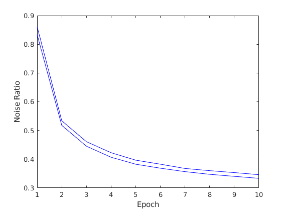
(a) DNN 1

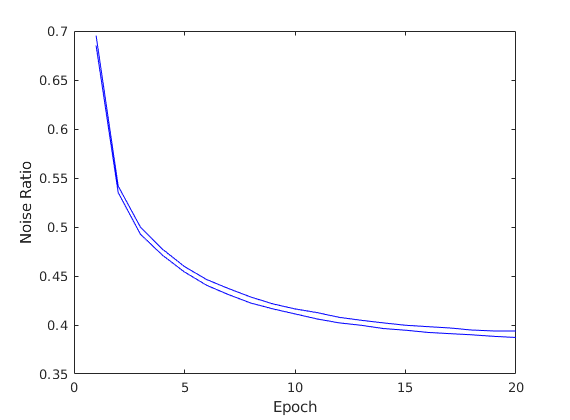
(b) DNN 2

Figure 8: Spread of the noise ratio for EKI(R) on DNN-(1,2). At the end of every epoch, when the noise is added, the upper bound is computed as $\|\bar{u}\|_{2}/\max_{j}\|\eta^{(j)}\|_{2}$. The lower bound is computed analogously.

      where $T$ is the number of steps needed to complete a cycle through the entire dataset and $\{\eta_{kT}^{(j)}\}_{j=1}^{J}$ is an i.i.d. sequence with $\eta_{kT}^{(1)}\sim\mu_{0}$. Note that because this randomization is only done after a full epoch, it is not clear how the noise should be scaled and thus we simply use the prior. This may not be the optimal thing to do, but we have found great numerical success with this strategy. Figure 8 shows the spread of the ratio of the parameters to the the noise $\|\bar{u}_{kT}\|/\|\eta^{(j)}_{kT}\|$. We see that relatively less noise is added as training continues. It may be possible to achieve better results by increasing the noise with time as to combat collapse. However, we do not perform such experiments. Furthermore we have found that this does not work well in the momentum case; hence all randomization for the momentum scheme is done according to the first point.

5. Expanding Ensemble: Numerical experiments show that using a small number of particles tends to have very good initial performance (one to two epochs) that quickly saturates. On the other hand, using a large number of particles does not do well to begin with but greatly outperforms small particle ensembles in the long run. Thus we use the idea of an expanding ensemble where we gradually add in new particles. This is done in the context of point (ii.) of the randomization section. Namely, at the end of an epoch, we compute the ensemble mean and create a new larger ensemble by randomizing around it.

Lastly we mention that, in many inverse problem applications, it is good practice to randomize the data for each particle at each step [44] namely map

$$\mathsf{y}\mapsto\mathsf{y}+\xi^{{}^{(j)}}_{k}$$

where $\{\xi^{(j)}_{k}\}_{j=1}^{J}$ is an i.i.d. sequence with $\xi^{(1)}_{k}\sim\pi$. However we have found that this does not work well for classification problems. This may be because the given classifications are correct and there is no actual noise in the data. Or it may be that we simply have not found a suitable measure from which to draw noise. We have not experimented in the case where the labels are noisy and leave this for future work.

5 Numerical Experiments

In the following set of experiments, we demonstrate the wide applicability of EKI on several machine learning tasks. All forward models we consider are some type of neural network, except for the semi-supervised learning case where we consider the construction in Example 2.2. We benchmark EKI against SGD and momentum SGD and do not consider any other first-order adaptive methods. Recent work has shown that their value is only marginal and the solutions they find may not generalize as well [85]. Furthermore we do not employ batch normalization as it is not clear how it should be incorporated with EKI methods. However, when batch normalization is necessary, we instead use the SELU nonlinearity, finding the performance to be essentially identical to batch normalization on problems where we have been able to compare.

The next five subsections are organized as follows. Subsection 5.1 contains the conclusions drawn from the experiments. In subsection 5.2, we describe the five data sets used in all of our experiments as well as the metrics used to evaluate the methods. Subsection 5.3 gives implementation details and assigns methods using different techniques their own name. In subsections 5.4, 5.5, and 5.6 we show the supervised, semi-supervised, and online learning experiments respectively. Since most of our experiments are supervised, we split subsection 5.4 based on the type of model used namely dense neural networks, convolutional neural networks, and recurrent neural networks respectively.

5.1 Conclusions From Numerical Experiments

The conclusions of our experiments are as follows:

• On supervised classification problems with a feed-forward neural network, EKI performs just as well as SGD even when the number of unknown parameters is very large (up to half a million) and the number of ensemble members is considerably smaller (by two orders of magnitude). Furthermore EKI seems more numerically stable than SGD, as seen in the smaller amount of oscillation in the test accuracy, and requires less hyper-parameter tuning. In fact, the only parameter we vary in our experiments is the number of ensemble members, and we do this simply to demonstrate its effect. However due to the large number of forward passes required at each EKI iteration, we have found the method to be significantly slower. This issue can be mitigated if each of the forward computations is parallelized across multiple processing units, as it often is in many industrial applications [33, 59, 58]. We leave such computational considerations for future work, as our current goal is simply to establish proof of concept. These experiments can be found in the first two subsections of section 5.4.

• On supervised classification problems with a recurrent neural network, EKI significantly outperforms SGD. This is likely due to the steep barriers that occur on the loss surface of recurrent networks [60, 4] which EKI may be able to avoid due to its noisy Jacobian estimates. These experiments can be found in the last subsection of section 5.4.

• On the semi-supervised learning problem we consider, EKI does not perform as well as state of the art (MCMC) [7], but performs better than the naive solution. However, even with a large number of ensemble members, EKI is much faster and computationally cheaper than MCMC, allowing applications to large scale problems. These experiments can be found in section 5.5.

• On online regression problems tackled with a recurrent neural network, EKI converges significantly faster and to a better solution than SGD with $\mathcal{O}(1)$ ensemble members. While the problems we consider are only simple, univariate time-series, the results demonstrate great promise for harder problems. It has long been known that recurrent neural networks are very hard to optimize with gradient-based techniques [60], so we are very hopeful that EKI can improve on current state of the art. Again, we leave such domain specific applications to future work. These experiments can be found in section 5.6.

5.2 Data Sets

We consider three data sets where the problem at hand is classification and two data sets where it is regression. For classification, two of the data sets are comprised of images and the third of voting histories. Our goal is to classify the image based on its content or classify the voting record based on party affiliation. For regression, both datasets are univariate time-series and our goal is to predict an unobserved part of the series. Figure 3 shows samples from each of the data sets.

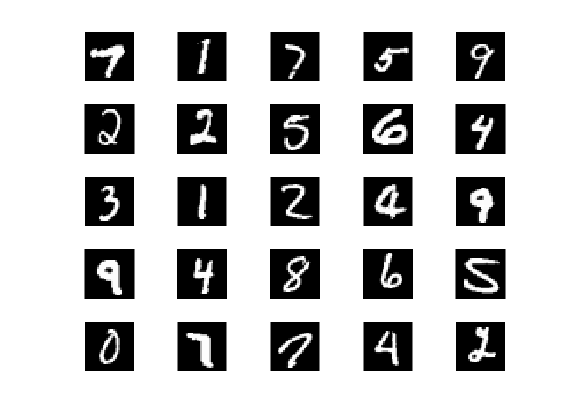
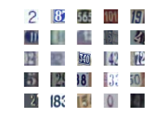
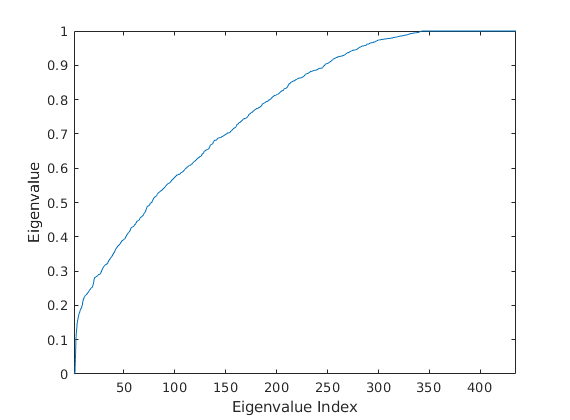
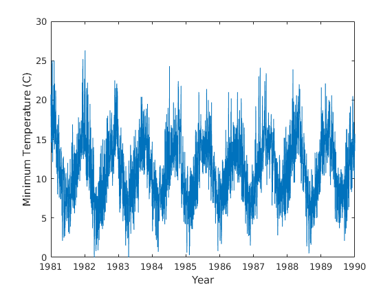
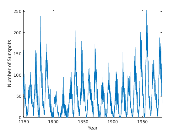
Figure 3: The five data sets used in numerical experiments. From left to right, the first are 25 samples from MNIST and SVHN respectively. The third shows the spectrum of graph Lalpacian for the Voting Records data set. The last two are the full time-series for the daily minimum temperatures in Melbourne and the monthly number of sunspots from Zürich respectively.

As outlined in section 2, the goal of learning is to find a model which generalizes well to unobserved data. Thus, to evaluate this criterion, we split all data sets into a training and a testing portion. The training portion is used when we let our ODE(s) evolve in time as described in section 4. The testing portion is used only to evaluate the model. In other contexts, the training set is further split to create a validation set, but, since we perform no hyper-parameter tuning, we omit this step. For classification, the metric we use is called test accuracy. This is the total number of correctly classified examples divided by the total number of examples in the test set. For regression, the metric we use is called test error. This is the average (across the test set) squared $\ell_{2}$-norm of the difference between the true value and our prediction.

5.2.1 Classification

The first data set we consider is MNIST [47]. It contains 70,000 images of hand-written digits. All examples are $28\times 28$ grayscale images and each is given a classification in $\{0,\dots,9\}$ depending on what digit appears in the image. Thus we consider $\mathcal{X}=\mathbb{R}^{28\times 28}\cong\mathbb{R}^{784}$ and $\mathcal{Y}=\mathbb{P}^{10}$. Each of the labels $y_{j}$ is a standard basis vector of $\mathbb{R}^{10}$ with the position of the 1 indicating the digit. We use 60,000 of the images for training and 10,000 for testing. Since grayscale values range from 0 to 255, all images are fist normalized to the range $[0,1]$ by point-wise dividing by 255. Treating all training images as a sequence of $60000\cdot 784$ numbers, their mean and standard deviation are computed. Each image (including the test set) is then again normalized via point-wise subtraction by the mean and point-wise division by the standard deviation. This data normalization technique is standard in machine learning.

The second image data set we consider is called SVHN [57]. It contains 99,289 natural images of cropped house numbers taken from Google Street View. All examples are $32\times 32$ RGB images and each is given a classification in $\{0,\dots,9\}$ depending on what digit appears in the image. Thus we consider $\mathcal{X}=\mathbb{R}^{3\times 32\times 32}\cong\mathbb{R}^{3072}$ and $\mathcal{Y}=\mathbb{P}^{10}$ with the labels again being basis vectors of $\mathbb{R}^{10}$. We use 73,257 of the images for training and 26,032 for testing. All values are first normalized to be in the range $[0,1]$. We then perform the same normalization as in MNIST, but this time per channel. That is, for all training images, we treat each color channel as a sequence of $73257\cdot 1024$ numbers, compute the mean and standard deviation then normalize each channel as before.

The last data set for classification we consider contains the voting record of the 435 U.S. House of Representatives members; see [6] and references therein. The votes were recorded in 1984 from the 98 United States Congress, 2 session. Each record is tied to a particular representative and is a vector in $\mathcal{X}=\mathbb{R}^{16}$ with each entry being $+1$, $-1$, or $0$ indicating a vote for, against, or abstain respectively. The labels live in $\mathcal{Y}=\mathbb{R}$ and are $+1$ or $-1$ indicating Democrat or Republican respectively. We use this data set only for semi-supervised learning and thus pick the amount of observed labels $|Z^{\prime}|=5$ with 2 Republicans and 3 Democrats. No normalization is performed. When computing the test accuracy, we do so over the entire data sets namely we do not remove the 5 observed records.

5.2.2 Regression

The first data set we consider for regression is a time series of the daily minimum temperatures (in Celsius) in Melbourne, Australia from January 1 1981 to December 31 1990 [19]. It contains 3650 total observations of which we use the first 3001 for training (up to March 22 1989) and the rest for testing. We consider $\mathcal{X}=\mathcal{Y}=\mathbb{R}$ by letting (in the training set) the data be the first 3000 observations and the labels be the 2 to 3001 observations i.e. a one-step-ahead split. The same is done for the testing set. The minimum and maximum values $x_{\text{min}}$, $x_{\text{max}}$ over the training set are computed and all data is transformed via

$$x_{j}\mapsto\frac{x_{j}-x_{\text{min}}}{x_{\text{max}}-x_{\text{min}}}.$$

This ensures the training set is in the range $[0,1]$ and the testing set will also be close to that range.

The second data set for regression is a time series containing the number of observed sunspots from Zürich, Switzerland during each month from January 1749 to December 1983 [1]. It contains 2820 observations of which we use the first 2301 for training (up to September 1915) and the rest for testing. The data is treated in exactly the same way as the temperatures data set.

5.3 Implementation Details

Having outlined many different strategies for performing EKI , we give methods using different techniques their own name so they are easily distinguishable. We refer to the techniques listed in section 4.3.3. All methods are initialized in the same way (with the prior constructed based on the model) and all use mini-batching. We refer to the forward Euler discretization of equation (13) as EKI and the momentum discretization, presented in section 4.2.1, of equation (13) as MEKI. When randomizing around the mean at the end of each epoch, we refer to the method as EKI(R). When randomizing the momenta at each step, we refer to the method as MEKI(R). Similarly, we call momentum SGD, MSGD. All methods use the time step described in section 4.3.3 with hyper-parameters $h_{0}=2$ and $\epsilon=0.5$ fixed. For any classification problem (except the Voting Records data set), all methods use the cross-entropy loss whose gradient is implemented with a slight correction for numerical stability. Namely, in the case of a single data point, we implement

$$(\nabla_{y^{\prime}}\mathcal{L}(\mathcal{G}(u),y))_{k}=-\frac{y_{k}}{(\mathcal{G}(u))_{k}+\delta}$$

where the constant $\delta:=0.005$ is fixed for all our numerical experiments. Otherwise the mean squared-error loss is used. All implementations are done using the PyTorch framework [61] on a single machine with an NVIDIA GTX 1080 Ti GPU.

5.4 Supervised Learning

5.4.1 Dense Neural Networks

In this section, we benchmark all of our proposed methods on the MNIST problem using four dense neural networks of increasing complexity. The four network architectures are outlined in Figure 4. This will allow us to compare the methods and pick a front runner for later experiments.

Dense Neural Networks
Name	Architecture	Parameters
DNN 1	784-10	7,850
DNN 2	784-100-10	79,510
DNN 3	784-300-100-10	266,610
DNN 4	784-500-300-100-10	573,910

Figure 4: Architectures of the four dense neural networks considered. All networks use a softmax thresholding and a ReLU nonlinearity.

We fix the ensemble size of all methods to $J=2000$ and the batch size to 600. SGD uses a learning rate of $0.1$ and all momentum methods use the constant $\lambda=0.9$. Figure 5 shows the final test accuracies for all methods while Figure 6 shows the accuracies at the end of each epoch. Due to memory constrains, we do not implement MEKI for DNN-(3,4). In general momentum SGD performs best, but EKI(R) trails closely. The momentum EKI methods have good initial performance but saturate. We make this clearer in a later experiment. Overall, we see that for networks with a relatively small number of parameters all EKI methods are comparable to SGD. However with a large number of parameters, randomization is needed. This effect is particularly dominant when the ensemble size is relatively small; as we later show, larger ensemble sizes can perform significantly better.

	DNN 1	DNN 2	DNN 3	DNN 4
SGD	0.9199	0.9735	0.9798	0.9818
MSGD	0.9257	0.9807	0.9830	0.9840
EKI	$\bar{u}$      0.9092 $u^{(j^{*})}$ 0.9114	$\bar{u}$      0.9398 $u^{(j^{*})}$ 0.9416	$\bar{u}$      0.9424 $u^{(j^{*})}$ 0.9432	$\bar{u}$      0.9404 $u^{(j^{*})}$ 0.9418
MEKI	$\bar{u}$      0.9094 $u^{(j^{*})}$ 0.9107	$\bar{u}$      0.9320 $u^{(j^{*})}$ 0.9332	n/a	n/a
EKI(R)	$\bar{u}$      0.9252 $u^{(j^{*})}$ 0.9260	$\bar{u}$      0.9721 $u^{(j^{*})}$ 0.9695	$\bar{u}$      0.9738 $u^{(j^{*})}$ 0.9716	$\bar{u}$      0.9741 $u^{(j^{*})}$ 0.9691
MEKI(R)	$\bar{u}$      0.9142 $u^{(j^{*})}$ 0.9162	$\bar{u}$      0.9509 $u^{(j^{*})}$ 0.9511	n/a	n/a

Figure 5: Final test accuracies of six training methods on four dense neural networks, solving the MNIST classification problem. Each bold number is the maximum across the column. For each EKI method we report the accuracy of the mean particle $\bar{u}$ and of the best performing particle in the ensemble $u^{(j^{*})}$.

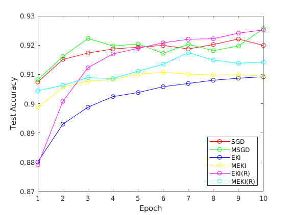
(a) DNN 1

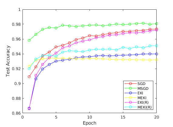
(b) DNN 2

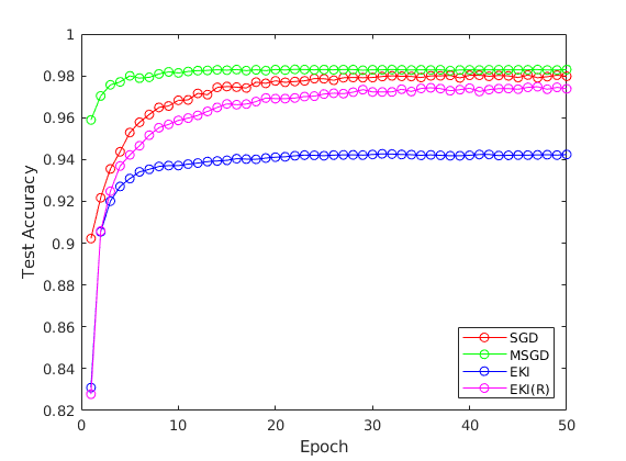
(c) DNN 3

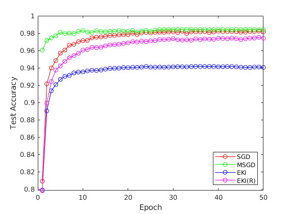
(d) DNN 4

Figure 6: Test accuracies per epoch of six training methods on four dense neural networks, solving the MNIST classification problem. For each EKI method the accuracy of the mean particle $\bar{u}$ is shown.

Figure 7 shows the test accuracies for each of the particles when using EKI on DNN-(1,2). We see that, the mean particle achieves roughly the average of the spread, as previously discussed. Our choice to use it as the final parameter estimate is simply for convenience. One may use all the particles in a carefully weighted scheme as an ensemble of networks and possibly achieve better results. Having many parameter estimates may also be advantageous when trying to avoid adversarial examples [22]. We leave these considerations to future work.

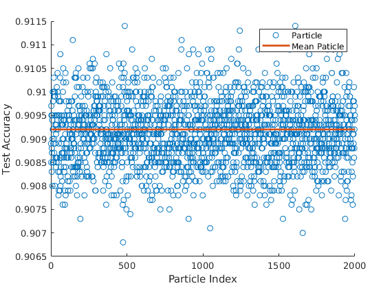
(a) DNN 1

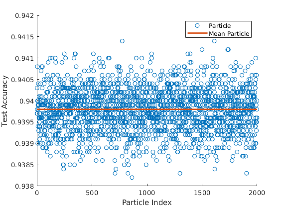
(b) DNN 2

Figure 7: Particle accuracies of EKI on DNN-(1,2) compared to the accuracy of the mean particle $\bar{u}$.

To better illustrate the effect of the ensemble size, we compare all EKI methods on DNN 2 with an ensemble size of $J=6000$. The accuracies are shown in Figure 9. We again observe that the momentum methods perform very well initially, but fall off with more training. This effect could be related to the specific time discretization method we use, but needs to be studied further theoretically and we leave this for future work. Note that with a larger ensemble, EKI is now comparable to SGD pointing out that remaining in the subspace spanned by the initial ensemble is a bottle neck for this method. On the other hand, when we randomize, the ensemble size is no longer so relevant. EKI(R) performs almost identically with 2,000 and with 6,000 ensemble members. Finding it to be the best method for these tasks, all experiments hereafter, unless stated otherwise, use EKI(R).

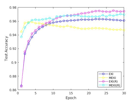
	First	Final
EKI	0.8661	0.9611
MEKI	0.9447	0.9471
EKI(R)	0.8652	0.9745
MEKI(R)	0.9373	0.9696

Figure 9: Comparison of the test accuracies of four EKI methods on DNN 2 with ensemble size $J=6000$.

5.4.2 Convolutional Neural Networks

For our experiments with CNN(s), we employ both MNIST and SVHN. Since MNIST is a fairly easy data set, we can use a simple architecture and still achieve almost perfect accuracy. We name the model CNN-MNIST and its specifics are given in the first column of Figure 10. SGD uses a learning rate of 0.05 while momentum SGD uses 0.01 and a momentum factor of 0.9. EKI(R) has a fixed ensemble size of $J=2000$. Figure 11 shows the results of training. We note that since CNN-MNIST uses ReLU and no batch normalization, SGD struggles to find a good descent direction in the first few epochs. EKI(R), on the other hand, does not have this issue and exhibits a smooth test accuracy curve that is consistent with all other experiments. In only 30 epochs, we are able to achieve almost perfect classification with EKI(R) slightly outperforming the SGD-based methods.

Recent work suggests that the effectiveness of batch normalization does not come from dealing with the internal covariate shift, but, in fact, comes from smoothing the loss surface [67]. The noisy gradient estimates in EKI can be interpreted as doing the same thing and is perhaps the reason we see smoother test accuracy curves. The contemporaneous work of Haber et al [25] further supports this point of view.

Convolutional Neural Networks
CNN-MNIST	CNN-1	CNN-2	CNN-3
Conv 16x3x3	Conv 16x3x3	Conv 16x3x3	Conv 16x3x3
Conv 16x3x3	Conv 16x3x3	Conv 16x3x3	Conv 16x3x3
		Conv 16x3x3	Conv 32x3x3
			Conv 32x3x3
			Conv 32x3x3
MaxPool 4x4 $(s=2)$	MaxPool 2x2	MaxPool 2x2	MaxPool 2x2
Conv 16x3x3	Conv 16x3x3	Conv 32x3x3	Conv 48x3x3
Conv 16x3x3	Conv 16x3x3	Conv 32x3x3	Conv 48x3x3
		Conv 32x3x3	Conv 48x3x3
			Conv 48x3x3
			Conv 48x3x3
MaxPool 4x4 $(s=2)$	MaxPool 2x2	MaxPool 2x2	MaxPool 2x2
Conv 12x3x3	Conv 32x3x3	Conv 48x3x3	Conv 64x3x3
Conv 12x3x3	Conv 32x3x3	Conv 48x3x3	Conv 64x3x3
		Conv 64x3x3	Conv 96x3x3
			Conv 96x3x3
			Conv 96x3x3
MaxPool 2x2	MaxPool 8x8	MaxPool 8x8	MaxPool 8x8
FC-10	FC-500	FC-500	FC-500
	FC-10	FC-10	FC-10

Figure 10: Architectures of 4 Convolutional Neural Networks with 6, 7, 10, 16 layers respectively from left to right. All convolutions use a padding of 1, making them dimension preserving since all kernel sizes are 3x3. CNN-MNIST is evaluated on the MNIST dataset and uses the ReLU nonlinearity. CNN-(1,2,3) are evaluated on the SVHN dataset and use the SELU nonlinearity. The convention $s=2$ refers to the stride of the max-pooling operation namely $\alpha=\beta=2$. All networks use a softmax thresholding.

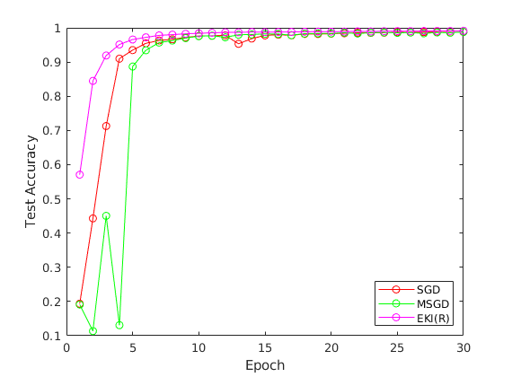
(a) CNN-MNIST

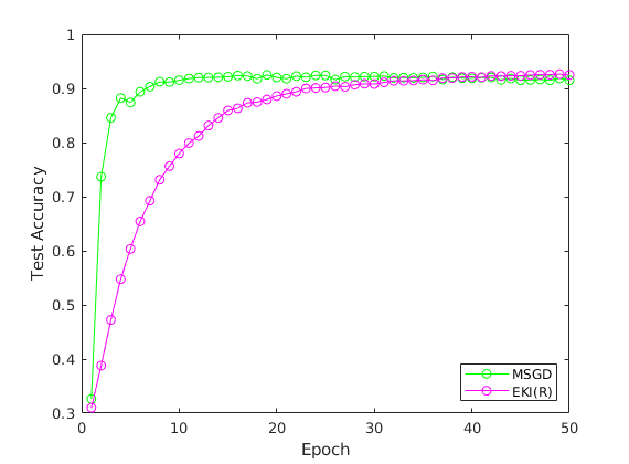
(b) CNN-1

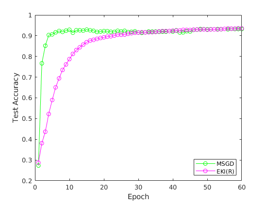
(c) CNN-2

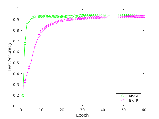
(d) CNN-3

	CNN-MNIST		CNN-1		CNN-2		CNN-3
	First	Final	First	Final	First	Final	First	Final
SGD	0.1936	0.9878	n/a	n/a	n/a	n/a	n/a	n/a
MSGD	0.1911	0.9880	0.3263	0.9150	0.2734	0.9324	0.1959	0.9414
EKI(R)	0.5708	0.9912	0.3100	0.9249	0.2874	0.9353	0.2668	0.9299

Figure 11: Comparison of the test accuracies of SGD and EKI(R) on four convolutional neural networks. SGD(M) refers to momentum SGD. CNN-MNIST is trained on the MNIST data set, while CNN-(1,2,3) are trained on the SVHN data set.

Next we experiment on the SVHN data set with three CNN(s) of increasing complexity. The architectures we use are inspired by those in [52], and are referred to as Fit-Nets because each layer is shallow (has a relatively small number of parameters), but the whole architecture is deep, reaching up to sixteen layers. The details for the models dubbed CNN-(1,2,3) are given in Figure 10. Such models are known to be difficult to train; for this reason, the papers [64, 52] present special initialization strategies to deal with the model complexities. We find that when using the SELU nonlinearity and no batch normalization, simple Xavier initialization works just as well. The results of training are presented in Figure 11. We benchmark only against momentum SGD as all previous experiments show it performs better than vanilla SGD. The method uses a learning rate of 0.01 and a momentum factor of 0.9. EKI(R) starts with $J=200$ ensemble members and expands by 200 at end the of each epoch until reaching a final ensemble of $J=5000$. For CNN-3, memory constraints allowed us to only expand up a final size of $J=2800$. All methods use a batch size of 500. We see that, in all three cases, EKI(R) and momentum SGD perform almost identically with EKI(R) slightly outperforming on CNN-(1,2), but falling off on CNN-3. This is likely due to the fact that CNN-3 has a large number of parameters and we were not able to provide a large enough ensemble size. This issue can be dealt with via parallelization by splitting the ensemble among the memory banks of separate processing units. We leave this consideration to future work.

5.4.3 Recurrent Neural Networks

For the classification task using a recurrent neural network, we return to the MNIST data set. Since recurrent networks work on time series data, we split each image along its rows, making a 28-dimensional time sequence with 28 entries, considering time going down from the top to the bottom of the image. More complex strategies have been explored in [84]. We use a two-layer recurrent network with 32 hidden units and a $\tanh$ nonlinearity, namely, in the notation of section 3.2,

$$F_{\theta}(z,q)=\sigma\left(W^{(2)}_{h}\sigma\left(W^{(1)}_{h}z+b_{h}^{(1)}+W_{x}^{(1)}q+b_{x}^{(1)}\right)+b_{h}^{(2)}+W_{x}^{(2)}q+b_{x}^{(2)}\right)$$

where $\sigma=\tanh$ and $W^{(1)}_{h},W^{(2)}_{h}\in\mathbb{R}^{32\times 32}$, $W_{x}^{(1)},W_{x}^{(2)}\in\mathbb{R}^{32\times 28}$. We look at only the last output of the network and thus only parametrize the last affine map $A_{28}$. Softmax thresholding is applied. The initial hidden state is always taken to be 0.

We train with a batch size of 600 and SGD uses a learning rate of 0.05. EKI(R) starts with an ensemble size of $J=1000$ and expands by 1,000 at the end of every epoch until $J=4000$ is reached. Figure 12 shows the result of training. EKI(R) performs significantly better than SGD and appears more reliable, overall, for this task.

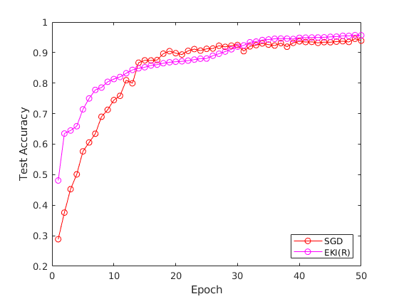
	First	Final
SGD	0.2825	0.9391
EKI(R)	0.4810	0.9566

Figure 12: Comparison of the test accuracies of EKI(R) and SGD on the MNIST data set with a two layer recurrent neural network.

5.5 Semi-supervised Learning

We proceed as in the construction of Example 2.2, using the Voting Records data set. For the affinity measure we pick [86, 7]

$$\eta(x,y)=\text{exp}\left(-\frac{\|x-y\|_{2}^{2}}{2(1.25)^{2}}\right)$$

and construct the graph Laplacian $\mathsf{L}(\mathsf{x})$. Its spectrum is shown in Figure 3. Further we let $\tau=0$ and $\alpha=1$, hence the prior covariance $C=(\mathsf{L}(\mathsf{x}))^{-1}$ is defined only on the subspace orthogonal to the first eigenvector of $\mathsf{L}(\mathsf{x})$. The most naive clustering algorithm that uses a graph Laplacian simply thresholds the eigenvector of $\mathsf{L}(\mathsf{x})$ that corresponds to the smalled non-zero eigenvalue (called the Fiedler vector) [83]. Its accuracy is shown in Figure 13. We found the best performing EKI method for this problem to simply be the vanilla version of the method i.e. no randomization or momentum. We use $J=1000$ ensemble members drawn from the prior and the mean squared-error loss. Its performance is only slightly better than the Fiedler vector as the particles quickly collapse to something close to the Fiedler vector. This is likely due to the fact that the initial ensemble is an i.i.d. sequence drawn from the prior hence EKI converges to a solution in the subspace orthogonal to the first eigenvector of $\mathsf{L}(\mathsf{x})$ which is close to the Fiedler vector, especially if the weights and other attendant hyper-parameters have been chosen so that the Fielder vector already classifies the labeled nodes correctly. On the other hand, the MCMC method detailed in [7] can explore outside of this subspace and achieve much better results. We note, however, that EKI is significantly cheaper and faster than MCMC and thus could be applied to much larger problems where MCMC is not computationally feasible.

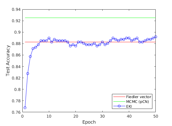
	Accuracy
Fiedler vector	0.8828
MCMC (pCN)	0.9252
EKI	0.8920

Figure 13: Comparison of the test accuracies of two semi-supervised learning algorithms to EKI on the Voting Records data set.

5.6 Online Learning

Finally we consider two online learning problems using a recurrent neural network. We employ two univariate time-series data sets: minimum daily temperatures in Melbourne, and the monthly number of sunspots observed from Zürich. For both, we use a single layer recurrent network with 32 hidden units and the $\tanh$ nonlinearity. The output is not thresholded i.e. $S=id$. At the initial time, we set the hidden state to 0 then use the hidden state computed in the previous step to initialize for the current step. This is an online problem as our algorithm only sees one data-label pair at a time. For OGD, we use a learning rate of 0.001 while, for EKI, we use $J=12$ ensemble members. Figure 14 shows the results of training as well as how well each of the trained model fits the test data. Notice that EKI converges much more quickly and to a slightly better solution than OGD in both cases. Furthermore, the model learned by EKI is able to better capture small scale oscillations. These are very promising results for the application of EKI to harder RNN problems.

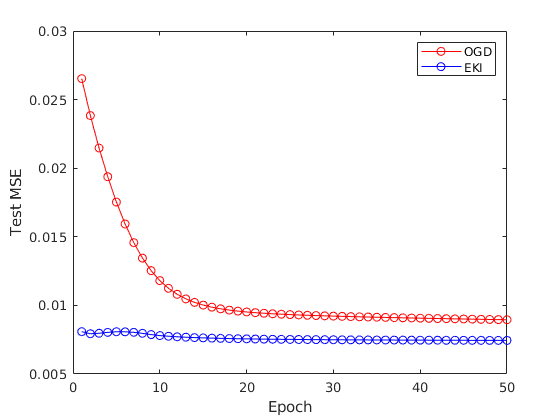
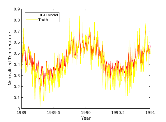
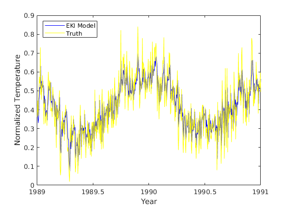
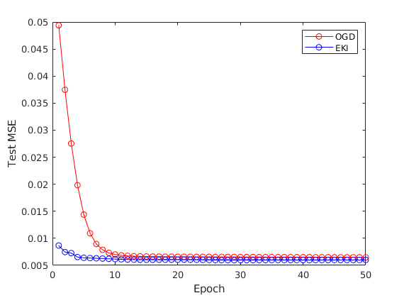
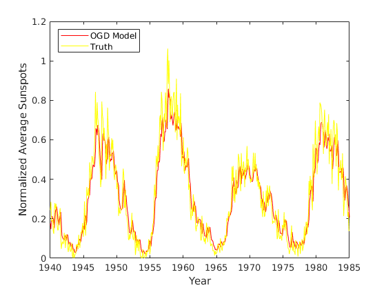
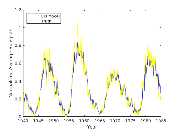
	Melbourne Temperatures		Zürich Sunspots
	First	Final	First	Final
OGD	$2.653\times 10^{-2}$	$8.954\times 10^{-3}$	$4.939\times 10^{-2}$	$6.480\times 10^{-3}$
EKI	$\mathbf{8.086\times 10^{-3}}$	$\mathbf{7.448\times 10^{-3}}$	$\mathbf{8.671\times 10^{-3}}$	$\mathbf{6.006\times 10^{-3}}$

Figure 14: Comparison of OGD and EKI on two online learning tasks with a recurrent neural network. The top row shows the minimum daily temperatures in Melbourne data set, while the bottom shows the number of sunspots observed each month from Zürich data set.

6 Conclusion and Future Directions

We have demonstrated that many machine learning problems can easily fit into the unified framework of Bayesian inverse problems. Within this framework, we apply Ensemble Kalman Inversion methods, for which we suggest suitable modifications, to tackle such tasks. Our numerical experiments suggest a wide applicability and competitiveness against the state-of-the-art for our schemes. The following directions for future search arise naturally from our work:

• Theoretical analysis of the momentum and general loss EKI methods as well as their possible application to physical inverse problems.

• GPU parallelization of EKI methods and its application to large scale machine learning tasks.

• Application of EKI methods to more difficult recurrent neural network problems as well as problems in reinforcement learning.

• Use of the entire ensemble of particle estimates to improve accuracy and possibly combat adversarial examples.

7 Acknowledgments

Both authors are supported, in part, by the US National Science Foundation (NSF) grant DMS 1818977, the US Office of Naval Research (ONR) grant N00014-17-1-2079, and the US Army Research Office (ARO) grant W911NF-12-2-0022.

References

References

- [1] D. Andrews and A. Herzberg, Data: a collection of problems from many fields for the student and research worker, Springer series in statistics, Springer, 1985.
- [2] L. J. Ba, R. Kiros, and G. E. Hinton, Layer normalization, CoRR, abs/1607.06450 (2016).
- [3] F. Bach and E. Moulines, Non-strongly-convex smooth stochastic approximation with convergence rate o (1/n), in Advances in neural information processing systems, 2013, pp. 773–781.
- [4] Y. Bengio, N. Boulanger-lew, R. Pascanu, and U. Montreal, Advances in optimizing recurrent networks, in In Acoustics, Speech and Signal Processing (ICASSP), 2013 IEEE International Conference on, 2013.
- [5] K. Bergemann and S. Reich, A mollified ensemble kalman filter, 136 (2010).
- [6] A. Bertozzi and A. Flenner, Diffuse interface models on graphs for classification of high dimensional data, Multiscale Modeling & Simulation, 10 (2012), pp. 1090–1118.
- [7] A. L. Bertozzi, X. Luo, A. M. Stuart, and K. C. Zygalakis, Uncertainty quantification in the classification of high dimensional data, CoRR, abs/1703.08816 (2017).
- [8] M. Binkowski, G. Marti, and P. Donnat, Autoregressive convolutional neural networks for asynchronous time series, CoRR, abs/1703.04122 (2017).
- [9] B. E. Boser, I. M. Guyon, and V. N. Vapnik, A training algorithm for optimal margin classifiers, in Proceedings of the Fifth Annual Workshop on Computational Learning Theory, COLT ’92, New York, NY, USA, 1992, ACM, pp. 144–152.
- [10] E. J. Candes and T. Tao, Near-optimal signal recovery from random projections: Universal encoding strategies?, IEEE Trans. Inf. Theor., 52 (2006), pp. 5406–5425.
- [11] M. Carreira-Perpinan and W. Wang, Distributed optimization of deeply nested systems, in Proceedings of the Seventeenth International Conference on Artificial Intelligence and Statistics, S. Kaski and J. Corander, eds., vol. 33 of Proceedings of Machine Learning Research, Reykjavik, Iceland, 22–25 Apr 2014, PMLR, pp. 10–19.
- [12] P. Chaudhari, A. Choromanska, S. Soatto, Y. LeCun, C. Baldassi, C. Borgs, J. T. Chayes, L. Sagun, and R. Zecchina, Entropy-sgd: Biasing gradient descent into wide valleys, CoRR, abs/1611.01838 (2016).
- [13] P. Chaudhari and S. Soatto, Stochastic gradient descent performs variational inference, converges to limit cycles for deep networks, CoRR, abs/1710.11029 (2017).
- [14] A. Dieuleveut, F. Bach, et al., Nonparametric stochastic approximation with large step-sizes, The Annals of Statistics, 44 (2016), pp. 1363–1399.
- [15] J. Duchi, E. Hazan, and Y. Singer, Adaptive subgradient methods for online learning and stochastic optimization, J. Mach. Learn. Res., 12 (2011), pp. 2121–2159.
- [16] M. Dunlop. Private Communication, 2017.
- [17] G. Evensen, The ensemble kalman filter: theoretical formulation and practical implementation, Ocean Dynamics, 53 (2003), pp. 343–367.
- [18] O. G. Ernst, B. Sprungk, and H.-J. Starkloff, Analysis of the ensemble and polynomial chaos kalman filters in bayesian inverse problems, 3 (2015).
- [19] L. Gil-Alana, Long memory behaviour in the daily maximum and minimum temperatures in melbourne, australia, Meteorologocal Applications, 11 (2006), pp. 319–328.
- [20] X. Glorot and Y. Bengio, Understanding the difficulty of training deep feedforward neural networks, in In Proceedings of the International Conference on Artificial Intelligence and Statistics (AISTATS’10). Society for Artificial Intelligence and Statistics, 2010.
- [21] I. Goodfellow, Y. Bengio, and A. Courville, Deep Learning, MIT Press, 2016. http://www.deeplearningbook.org.
- [22] I. Goodfellow, J. Shlens, and C. Szegedy, Explaining and harnessing adversarial examples, in International Conference on Learning Representations, 2015.
- [23] B. Graham, Fractional max-pooling, CoRR, abs/1412.6071 (2014).
- [24] C. Gulcehre, K. Cho, R. Pascanu, and Y. Bengio, Learned-norm pooling for deep feedforward and recurrent neural networks, in Proceedings of the European Conference on Machine Learning and Knowledge Discovery in Databases - Volume 8724, ECML PKDD 2014, Berlin, Heidelberg, 2014, Springer-Verlag, pp. 530–546.
- [25] E. Haber, F. Lucka, and L. Ruthotto, Never look back - a modified enkf method and its application to the training of neural networks without back propagation, CoRR, abs/1805.08034 (2018).
- [26] S. S. Haykin, Kalman Filtering and Neural Networks, John Wiley & Sons, Inc., New York, NY, USA, 2001.
- [27] K. He, X. Zhang, S. Ren, and J. Sun, Spatial pyramid pooling in deep convolutional networks for visual recognition, in Computer Vision – ECCV 2014, D. Fleet, T. Pajdla, B. Schiele, and T. Tuytelaars, eds., Cham, 2014, Springer International Publishing, pp. 346–361.
- [28] G. Hinton and R. Salakhutdinov, Reducing the dimensionality of data with neural networks, Science, 313 (2006), pp. 504 – 507.
- [29] S. Hochreiter, Y. Bengio, P. Frasconi, and J. Schmidhuber, Gradient flow in recurrent nets: the difficulty of learning long-term dependencies, in A Field Guide to Dynamical Recurrent Neural Networks, Kremer and Kolen, eds., IEEE Press, 2001.
- [30] S. Hochreiter and J. Schmidhuber, Long short-term memory, Neural Comput., 9 (1997), pp. 1735–1780.
- [31] A. E. Hoerl and R. W. Kennard, Ridge regression: Biased estimation for nonorthogonal problems, Technometrics, 12 (1970), pp. 55–67.
- [32] K. Hornik, Approximation capabilities of multilayer feedforward networks, Neural Netw., 4 (1991), pp. 251–257.
- [33] P. Houtekamer, B. He, and H. L. Mitchell, Parallel implementation of an ensemble kalman filter, 142 (2014).
- [34] M. Iglesias, Y. Lu, and A. Stuart, A bayesian level set method for geometric inverse problems, Interfaces and Free Boundaries, 18 (2016), pp. 181–217.
- [35] M. A. Iglesias, K. J. H. Law, and A. M. Stuart, Ensemble Kalman methods for inverse problems, Inverse Problems, 29 (2013), p. 045001.
- [36] S. Ioffe and C. Szegedy, Batch normalization: Accelerating deep network training by reducing internal covariate shift, in Proceedings of the 32Nd International Conference on International Conference on Machine Learning - Volume 37, ICML’15, JMLR.org, 2015, pp. 448–456.
- [37] M. Jordan, On gradient-based optimization: Accelerated, distributed, asynchronous and stochastic, in ACM SIGMETRICS Performance Evaluation Review, vol. 45, ACM, 2017, pp. 58–58.
- [38] B. Kay and R. Sebastian, A localization technique for ensemble kalman filters, Quarterly Journal of the Royal Meteorological Society, 136, pp. 701–707.
- [39] J. Kiefer and J. Wolfowitz, Stochastic estimation of the maximum of a regression function, Ann. Math. Statist., 23 (1952), pp. 462–466.
- [40] D. P. Kingma and J. Ba, Adam: A method for stochastic optimization, CoRR, abs/1412.6980 (2014).
- [41] G. Klambauer, T. Unterthiner, A. Mayr, and S. Hochreiter, Self-normalizing neural networks, in Advances in Neural Information Processing Systems 30, I. Guyon, U. V. Luxburg, S. Bengio, H. Wallach, R. Fergus, S. Vishwanathan, and R. Garnett, eds., Curran Associates, Inc., 2017, pp. 971–980.
- [42] P. Kloeden and M. Rasmussen, Nonautonomous Dynamical Systems, vol. 176, 08 2011.
- [43] A. Krizhevsky, I. Sutskever, and G. E. Hinton, Imagenet classification with deep convolutional neural networks, in Advances in Neural Information Processing Systems 25, F. Pereira, C. J. C. Burges, L. Bottou, and K. Q. Weinberger, eds., Curran Associates, Inc., 2012, pp. 1097–1105.
- [44] K. Law, A. Stuart, and K. Zygalakis, Data assimilation: A mathematical introduction, vol. 62 of Texts in Applied Mathematics, Springer, Cham, 2015.
- [45] Y. LeCun, Y. Bengio, and G. E. Hinton, Deep learning, Nature, 521 (2015), pp. 436–444.
- [46] Y. Lecun, L. Bottou, Y. Bengio, and P. Haffner, Gradient-based learning applied to document recognition, in Proceedings of the IEEE, 1998, pp. 2278–2324.
- [47] Y. LeCun and C. Cortes, MNIST handwritten digit database, (2010).
- [48] J. D. Lee, M. Simchowitz, M. I. Jordan, and B. Recht, Gradient descent only converges to minimizers, in Conference on Learning Theory, 2016, pp. 1246–1257.
- [49] G. J. S. Litjens, T. Kooi, B. E. Bejnordi, A. A. A. Setio, F. Ciompi, M. Ghafoorian, J. A. W. M. van der Laak, B. van Ginneken, and C. I. Sánchez, A survey on deep learning in medical image analysis, CoRR, abs/1702.05747 (2017).
- [50] C. D. Manning and H. Schütze, Foundations of Statistical Natural Language Processing, MIT Press, Cambridge, MA, USA, 1999.
- [51] P. McCullagh and J. Nelder, Generalized Linear Models, Second Edition, Chapman and Hall/CRC Monographs on Statistics and Applied Probability Series, Chapman & Hall, 1989.
- [52] D. Mishkin and J. Matas, All you need is a good init, CoRR, abs/1511.06422 (2015).
- [53] K. P. Murphy, Machine Learning: A Probabilistic Perspective, The MIT Press, 2012.
- [54] J. Nagi, F. Ducatelle, G. A. D. Caro, D. Ciresan, U. Meier, A. Giusti, F. Nagi, J. Schmidhuber, and L. M. Gambardella, Max-pooling convolutional neural networks for vision-based hand gesture recognition, 2011.
- [55] V. Nair and G. E. Hinton, Rectified linear units improve restricted boltzmann machines, in Proceedings of the 27th International Conference on International Conference on Machine Learning, ICML’10, USA, 2010, Omnipress, pp. 807–814.
- [56] Y. Nesterov, A method of solving a convex programming problem with convergence rate o(1/k2), Soviet Mathematics Doklady, 27 (1983), pp. 372–376.
- [57] Y. Netzer, T. Wang, A. Coates, A. Bissacco, B. Wu, and A. Y. Ng, Reading digits in natural images with unsupervised feature learning, (2011).
- [58] E. D. Niño, A. Sandu, and X. Deng, A parallel implementation of the ensemble kalman filter based on modified cholesky decomposition, CoRR, abs/1606.00807 (2016).
- [59] E. D. Nino-Ruiz and A. Sandu, An efficient parallel implementation of the ensemble kalman filter based on shrinkage covariance matrix estimation, in Proceedings of the 2015 IEEE 22Nd International Conference on High Performance Computing Workshops (HiPCW), HIPCW ’15, Washington, DC, USA, 2015, IEEE Computer Society, pp. 54–54.
- [60] R. Pascanu, T. Mikolov, and Y. Bengio, On the difficulty of training recurrent neural networks, in Proceedings of the 30th International Conference on International Conference on Machine Learning - Volume 28, ICML’13, JMLR.org, 2013, pp. III–1310–III–1318.
- [61] A. Paszke, S. Gross, S. Chintala, G. Chanan, E. Yang, Z. DeVito, Z. Lin, A. Desmaison, L. Antiga, and A. Lerer, Automatic differentiation in pytorch, in NIPS-W, 2017.
- [62] C. E. Rasmussen and C. K. Williams, Gaussian process for machine learning, MIT press, 2006.
- [63] H. Robbins and S. Monro, A stochastic approximation method, Ann. Math. Statist., 22 (1951), pp. 400–407.
- [64] A. Romero, N. Ballas, S. E. Kahou, A. Chassang, C. Gatta, and Y. Bengio, Fitnets: Hints for thin deep nets, in In Proceedings of ICLR, 2015.
- [65] D. W. Ruck, S. K. Rogers, M. Kabrisky, M. E. Oxley, and B. W. Suter, The multilayer perceptron as an approximation to a bayes optimal discriminant function, IEEE Transactions on Neural Networks, 1 (1990), pp. 296–298.
- [66] D. E. Rumelhart, G. E. Hinton, and R. J. Williams, Neurocomputing: Foundations of research, MIT Press, Cambridge, MA, USA, 1988, ch. Learning Representations by Back-propagating Errors, pp. 696–699.
- [67] S. Santurkar, D. Tsipras, A. Ilyas, and A. Madry, How does batch normalization help optimization? (no, it is not about internal covariate shift), CoRR, abs/1805.11604 (2018).
- [68] C. Schillings and A. M. Stuart, Analysis of the ensemble kalman filter for inverse problems, SIAM J. Numerical Analysis, 55 (2017), pp. 1264–1290.
- [69] J. Schmidhuber, Learning complex, extended sequences using the principle of history compression, Neural Comput., 4 (1992), pp. 234–242.
- [70] M. Schmidt, N. Le Roux, and F. Bach, Minimizing finite sums with the stochastic average gradient, Mathematical Programming, 162 (2017), pp. 83–112.
- [71] A. Stuart and A. R. Humphries, Dynamical systems and numerical analysis, vol. 2, Cambridge University Press, 1998.
- [72] W. Su, S. Boyd, and E. Candes, A differential equation for modeling nesterov’s accelerated gradient method: Theory and insights, in Advances in Neural Information Processing Systems 27, Z. Ghahramani, M. Welling, C. Cortes, N. D. Lawrence, and K. Q. Weinberger, eds., Curran Associates, Inc., 2014, pp. 2510–2518.
- [73] F. P. Such, V. Madhavan, E. Conti, J. Lehman, K. O. Stanley, and J. Clune, Deep neuroevolution: Genetic algorithms are a competitive alternative for training deep neural networks for reinforcement learning, CoRR, abs/1712.06567 (2017).
- [74] I. Sutskever, Training Recurrent Neural Networks, PhD thesis, Toronto, Ont., Canada, Canada, 2013. AAINS22066.
- [75] I. Sutskever, J. Martens, G. Dahl, and G. Hinton, On the importance of initialization and momentum in deep learning, in Proceedings of the 30th International Conference on International Conference on Machine Learning - Volume 28, ICML’13, JMLR.org, 2013, pp. III–1139–III–1147.
- [76] I. Sutskever, O. Vinyals, and Q. V. Le, Sequence to sequence learning with neural networks, in Proceedings of the 27th International Conference on Neural Information Processing Systems - Volume 2, NIPS’14, Cambridge, MA, USA, 2014, MIT Press, pp. 3104–3112.
- [77] C. Szegedy, W. Zaremba, I. Sutskever, J. Bruna, D. Erhan, I. Goodfellow, and R. Fergus, Intriguing properties of neural networks, in International Conference on Learning Representations, 2014.
- [78] G. Taylor, R. Burmeister, Z. Xu, B. Singh, A. Patel, and T. Goldstein, Training neural networks without gradients: A scalable admm approach, in Proceedings of the 33rd International Conference on International Conference on Machine Learning - Volume 48, ICML’16, JMLR.org, 2016, pp. 2722–2731.
- [79] Y. H. Tsai, O. C. Hamsici, and M. H. Yang, Adaptive region pooling for object detection, in 2015 IEEE Conference on Computer Vision and Pattern Recognition (CVPR), June 2015, pp. 731–739.
- [80] D. Ulyanov, A. Vedaldi, and V. S. Lempitsky, Instance normalization: The missing ingredient for fast stylization, CoRR, abs/1607.08022 (2016).
- [81] V. N. Vapnik, The Nature of Statistical Learning Theory, Springer-Verlag, Berlin, Heidelberg, 1995.
- [82] C. R. Vogel, Computational Methods for Inverse Problems, Society for Industrial and Applied Mathematics, Philadelphia, PA, USA, 2002.
- [83] U. von Luxburg, A tutorial on spectral clustering, Statistics and Computing, 17 (2007), pp. 395–416.
- [84] J. Wang, Y. Yang, J. Mao, Z. Huang, C. Huang, and W. Xu, Cnn-rnn: A unified framework for multi-label image classification, in 2016 IEEE Conference on Computer Vision and Pattern Recognition (CVPR), June 2016, pp. 2285–2294.
- [85] A. C. Wilson, R. Roelofs, M. Stern, N. Srebro, and B. Recht, The marginal value of adaptive gradient methods in machine learning, in Advances in Neural Information Processing Systems 30, I. Guyon, U. V. Luxburg, S. Bengio, H. Wallach, R. Fergus, S. Vishwanathan, and R. Garnett, eds., Curran Associates, Inc., 2017, pp. 4148–4158.
- [86] L. Zelnik-manor and P. Perona, Self-tuning spectral clustering, in Advances in Neural Information Processing Systems 17, L. K. Saul, Y. Weiss, and L. Bottou, eds., MIT Press, 2005, pp. 1601–1608.
- [87] S. Zhang, A. Choromanska, and Y. LeCun, Deep learning with elastic averaging sgd, in Proceedings of the 28th International Conference on Neural Information Processing Systems - Volume 1, NIPS’15, Cambridge, MA, USA, 2015, MIT Press, pp. 685–693.