Computation of Stability Radii for Large-Scale Dissipative Hamiltonian Systems
Abstract
A linear time-invariant dissipative Hamiltonian (DH) system ,
with a skew-Hermitian , an Hermitian positive semi-definite , and an Hermitian positive definite ,
is always Lyapunov stable and under weak further conditions even asymptotically stable.
In various applications there is uncertainty
on the system matrices , and it is desirable to know whether the system remains
asymptotically stable uniformly against all possible uncertainties within a given perturbation set. Such robust stability
considerations motivate the concept of stability radius for DH systems, i.e., what is the maximal
perturbation permissible to the coefficients , while preserving the asymptotic stability.
We consider two stability radii, the unstructured one where
are subject to unstructured perturbation, and the structured one where the perturbations preserve the DH structure.
We employ characterizations for these radii that have been
derived recently in [SIAM J. Matrix Anal. Appl., 37, pp. 1625-1654, 2016] and propose new algorithms to compute
these stability radii for large scale problems by tailoring subspace frameworks that
are interpolatory and guaranteed to converge at a super-linear rate in theory.
At every iteration, they first solve a reduced problem and then expand
the subspaces in order to attain certain Hermite interpolation properties between the full and
reduced problems. The reduced problems are solved by means of the adaptations
of existing level-set algorithms for -norm computation in the unstructured case,
while, for the structured radii, we benefit from algorithms that approximate the
objective eigenvalue function with a piece-wise quadratic global underestimator.
The performance of the new approaches is illustrated with several examples including a system
that arises from a finite-element modeling of an industrial disk brake.
Key words. Linear Time-Invariant Dissipative Hamiltonian System, Port-Hamiltonian system, Robust Stability, Stability Radius, Eigenvalue Optimization, Subspace Projection, Structure Preserving Subspace Framework,
Hermite Interpolation.
AMS subject classifications. 65F15, 93D09, 93A15, 90C26
1 Introduction
Linear time-invariant Dissipative Hamiltonian (DH) systems are dynamical systems of the form
| (1.1) |
They arise as homogeneous part of port-Hamiltonian (PH) systems of the form
| (1.2) |
when the input is and the output is not considered. Here is an Hermitian positive definite matrix (denoted as ), is a skew-Hermitian matrix associated with the energy flux of the system, is the Hermitian positive semi-definite (denoted by ) dissipation matrix of the system, are the port matrices, and describes the direct feed-through from input to output. The function (called Hamiltonian function) describes the total internal energy of the system. Here and elsewhere denotes the conjugate transpose of a complex matrix .
PH and DH systems play an essential role in most areas of science and engineering, see e.g. [12, 20], due to their very important structural properties; e.g., they allow modularized modeling and easy model reduction via Galerkin projection. An important structural property is that DH systems are automatically Lyapunov stable, i.e., all eigenvalues of are in the closed left half of the complex plane, and those on the imaginary axis are semisimple, see [15]. However, DH systems are not necessarily asymptotically stable, since may have purely imaginary eigenvalues, e.g., when the dissipation matrix vanishes, then all eigenvalues are purely imaginary. If a DH system is Lyapunov stable but not asymptotically stable, then arbitrarily small unstructured perturbations (such as rounding errors) may cause the system to become unstable.
These issues are our motivation to analyse whether a DH system is robustly asymptotically stable, i.e., whether small (structured or unstructured) perturbations keep it asymptotically stable.
Example 1.1.
Disk brake squeal is a well-known problem in mechanical engineering. It occurs due to self-excited vibrations caused by instability at the pad-rotor interface [1]. The transition from stability to instability of the brake system is generally examined by finite element (FE) analysis of the system. In [7] FE models resulting for disk brakes are derived in form of second order differential equations
| (1.3) |
with large and sparse coefficient matrixes , , and , where and depend on the rotational speed of the disk, and have the form
with representing material, friction-induced damping matrices, corresponding to elastic, geometric stiffness matrices, respectively. Here, and , whereas . (The function represents a forcing term or control, but for the stability analysis one may assume that , which we assume in the following.) The incorporation of gyroscopic effects, modeled by the term , with , and circulatory effects, modeled by an unsymmetric term gives rise to a system
| (1.4) |
or in first order representation , where
| (1.5) |
Straightforward manipulations yields a system
| (1.6) |
with , where
| (1.7) |
In the absence of the circulatory effects, i.e., when , the system in (1.6) is a DH system and as a result it is Lyapunov stable and typically even asymptotically stable. However, small circulatory effects, i.e., perturbations by a non-symmetric of small norm, may result in instability.
Asymptotic stability of a general linear dynamical system in the presence of uncertainty can only be guaranteed when the system has a reasonable distance to instability, i.e., to systems with purely imaginary eigenvalues. Hence, an estimation of the distance to instability, which is an optimization problem over admissible perturbations, is an important ingredient of a proper stability analysis.
In this paper we focus on the stability analysis of large-scale (and typically sparse) DH systems of the form (1.1) in the presence of uncertainties in the coefficients. Considering perturbations in one of the coefficient matrices , , of (1.1), in [15] characterizations for several structured distances to instability were derived under restricted perturbations of the form , with restriction matrices and of full column rank and full row rank, respectively, allowing selected parts of the matrices to be unperturbed. We will use an adaptation of the subspace framework introduced in [2], based on model order reduction techniques to compute the stability radii using the characterizations in [15].
The paper is organized as follows. Section 2 provides formal definitions of the structured and unstructured stability radii, and in Section 3 we briefly recall the characterizations of these stability radii derived in [15]. Section 4 proposes subspace frameworks for computing the unstructured stability radii problems exploiting these characterizations. The performance of the proposed frameworks for the unstructured stability radii is illustrated via the disk brake example and several synthetic examples in Section 4.3. Finally, Section 5 focuses on the structured stability radius when only is subject to Hermitian perturbations. We first discuss how small-scale problems can be solved in Section 5.1. A new structured subspace framework is discussed in Section 5.2 followed by several numerical examples in Section 5.3.
2 Unstructured and Structured Stability Radii
In [15] computable formulas for DH systems of the form (1.1) are derived using several notions of unstructured and structured stability radii. In this section we briefly recall the main definitions and results from [15] for restricted perturbations in one of the following forms.
| (2.1) |
In the following denotes the imaginary axis in the complex plane, the spectrum of a matrix , and the spectral norm.
Definition 2.1.
Consider a DH system of the form (1.1) and suppose that and are given full rank restriction matrices.
-
(i)
The unstructured restricted stability radius with respect to perturbations of under the restriction matrices , is defined by
-
(ii)
The unstructured restricted stability radius with respect to perturbations of under the restriction matrices , is defined by
-
(iii)
The unstructured restricted stability radius with respect to perturbations of under the restriction matrices , is defined by
Example 2.2.
Consider again Example 1.1. Here it is of interest to know whether (for given ) the norm of the non-symmetric matrix is tolerable to preserve the asymptotic stability of the DH system in (1.6) without the circulatory effects. The relevant stability radius for a specified is given by
| (2.2) |
where
Hence, the stability radius in (2.2) corresponds to the unstructured stability radius with the restriction matrices and with blocks.
Furthermore, in the definition of the skew-Hermitian perturbations are more influential on the imaginary parts of its eigenvalues, whereas the Hermitian perturbations are more effective in moving its eigenvalues towards the imaginary axis. This leads us to the consideration of the stability radius
| (2.3) |
with
Examples such as Example 2.2 motivate the following definition of the structured stability radius in [15].
Definition 2.3.
Consider a DH system of the form (1.1) and suppose that is a given restriction matrix. The structured restricted stability radius with respect to Hermitian perturbations of under the restriction is defined by
| (2.4) |
3 Characterizations for Stability Radii
The numerical techniques that we will derive for the computation of the unstructured and structured stability radii exploit eigenvalue or singular value optimization characterizations derived in [15].
Theorem 3.1.
For an asymptotically stable DH system of the form (1.1) and restriction matrices , the following assertions hold:
-
(i)
The unstructured stability radius is finite if and only if is not identically zero if and only if is finite. If is finite, then we have
(3.1) -
(ii)
The unstructured stability radius is finite if and only if is not identically zero for all . If is finite, then we have
(3.2)
For the structured stability radius and Hermitian perturbations of the following result is obtained in [15].
Theorem 3.2.
For an asymptotically stable DH system of the form (1.1), and a restriction matrix of full column rank, let
-
1.
for a given such that is invertible,
-
2.
be a lower triangular Cholesky factor of
,
i.e., is a lower triangular matrix satisfying ,
-
3.
,
-
4.
, where .
Then is finite, and given by
where denotes the smallest eigenvalue of its Hermitian matrix argument, and the inner supremum is attained if and only if is indefinite.
The characterization in [15] is presented in a slightly different form. In particular, it is stated in terms of an orthonormal basis for the kernel of . It turns out that does not have to be orthonormal, rather the theorem can be stated in terms of any basis for the kernel of . In Theorem 3.2, we have employed a particular basis that simplifies the formulas and facilitates the computation.
4 Computation of the Unstructured Stability Radii for Large-Scale Problems
In this section we study the computation of unstructured stability radii for large-scale DH systems using the characterizations of , , given in Theorem 3.1. One easily observes that
can be viewed as restrictions of transfer functions of control systems to the imaginary axis. To be precise, setting , and , the matrix-valued function becomes
| (4.1) |
which can be considered as the transfer function of the system
| (4.2) |
on the imaginary axis. Theorem 3.1 suggests that if is not identically zero, then and are finite, and characterized by
| (4.3) |
where denotes the -norm of , and denotes the maximal singular value.
For the stability radius , consideration of , by setting , and , leads us to a similar characterization.
4.1 A Subspace Framework
Recently, in [2], a subspace framework for the computation of the -norm of a large-scale system has been proposed, which is inspired from model order reduction techniques, and has made the computation of -norms feasible for very large control systems. We will now discuss how to use these techniques for the computation of the unstructured stability radii , , in the large-scale setting.
To briefly summarize the iterative procedure in the subspace framework of [2], let us assume that in iteration , two subspaces and of equal dimension have been determined, as well as matrices and whose columns span orthonormal bases for these subspaces. Applying a Petrov-Galerkin projection to system (4.2), restricts the state to , i.e., in (4.2) we replace by , and imposes that the residual after this restriction is orthogonal to . This projection gives rise to a reduced order system
| (4.4) |
with
| (4.5) |
Then the -norm of a transfer function in (4.2) can be approximated by computing the -norm of
for instance by employing the method in [4] or [5], in particular, by computing . This is computationally cheap if the dimensions of are small. Once has been computed, then the subspaces and are expanded into larger subspaces and in such a way that the corresponding reduced transfer function satisfies the Hermite interpolation conditions
| (4.6) |
where denotes the derivative of with respect to . Denoting the image space of a matrix by by , it is shown in [2] that
more specifically the inclusions
ensure that the Hermite interpolation conditions (4.6) are satisfied. The procedure is then repeated with the expanded subspaces , . In [2], it is shown that the sequence converges at a super-linear rate and satisfies
for .
A disadvantage of this general approach is that even if has DH structure, this is not necessarily true for , so it cannot be guaranteed from the structure that the reduced system is stable. In the next section we modify the procedure of [2] to preserve the DH structure.
4.2 A Structure Preserving Subspace Framework
In this subsection we derive an interpolating, DH structure preserving version of the robust subspace projection framework. Structure preserving subspace projection methods in the context of model order reduction of large-scale PH and DH systems have been proposed in [10, 11, 17, 18, 21, 22]. Our approach is inspired by [10] and uses a general interpolation result from [6].
Theorem 4.1.
Let be the transfer function for a full order system as in (4.2), and let be the transfer function for the reduced system defined by (4.4), (4.5).
-
(i)
(Right Tangential Interpolation) For given and , if
(4.7) and is such that , then we have
(4.8) provided that both and are invertible.
-
(ii)
(Left Tangential Interpolation) For a given and , if
(4.9) and is such that , then we have
(4.10) provided that both and are invertible.
4.2.1 Computation of and
The computation of involves the maximization of the largest singular value of the transfer function associated with the system
| (4.11) |
on the imaginary axis. We make use of Theorem 4.1 to obtain a reduced order system satisfying the interpolation conditions (4.8) while retaining the structure in (4.11). We, in particular, employ right tangential interpolation for a given and , and choose as any subspace satisfying (4.7). Let us also define , , so that
i.e., is an oblique projector onto .
The matrices of the reduced system (4.4), (4.5) for these choices of and then satisfy
| (4.12) |
where , , and . Additionally, , where , and .
This construction leads to the following result of [10].
Theorem 4.2.
Consider a linear system of the form (4.11) with transfer function . Furthermore, for a given point and a given tangent direction , suppose that is a matrix with orthonormal columns such that
Define and set
| (4.13) |
Then the resulting reduced order model
| (4.14) |
is a DH system with transfer function
| (4.15) |
that satisfies
| (4.16) |
where denotes the -th derivative of at the point .
According to Theorem 4.2, for a given , setting
where
| (4.17) |
we obtain and and thus the Hermite interpolation conditions
| (4.18) |
are satisfied, which suggest the use of the reduced system in the greedy subspace framework outlined in Algorithm 1.
In line 5 of every iteration, the subspace framework computes the -norm of a reduced system, in particular it computes the point on the imaginary axis where this -norm is attained. Then the current left and right subspaces are expanded in a way so that the resulting reduced system still has DH structure and its transfer function Hermite interpolates the original transfer function at . Since the Hermite interpolation conditions (4.18) are satisfied at at the end of iteration , the rate-of-convergence analysis in [2] applies to deduce a superlinear rate-of-convergence for the sequence .
The computationally most expensive part of Algorithm 1 is in lines 2 and 6, where many linear systems with possibly many right hand sides have to be solved. If this is done with a direct solver, then for each value one factorization of the matrix has to be performed. For large values of , the computation time is usually dominated by these factorizations. In contrast to this, the solution of the reduced problem in line 5 can be achieved (for small systems) by means of the efficient algorithm in [4, 5].
4.2.2 Computation of
To compute the stability radius in the large-scale setting, we employ left tangential interpolations (i.e., part (ii) of Theorem 4.1).
In this case is the reciprocal of the -norm of the transfer function corresponding to the system
| (4.19) |
To obtain a reduced system which has the same structure as (4.19) and has a transfer function that satisfies for a given point and a direction , let us choose so as to satisfy the condition in (4.9) for , and . Furthermore, we set
as well as , . The matrix is chosen to satisfy
so that is an oblique projector onto .
In (4.19), setting , , , let us investigate the matrices of the corresponding reduced system defined by (4.4), (4.5). Specifically, we have that
where, in the third equality, we employ , or equivalently . Hence, defining , , , we obtain a DH system with . We also have
with , and . These constructions lead to the following analogue of Theorem 4.2.
Theorem 4.3.
Consider a linear system of the form (4.19) with the transfer function . For a given point and a direction , suppose that is a matrix with orthonormal columns such that
for . Letting , and
| (4.20) |
the resulting reduced order system
| (4.21) |
is such that is dissipative Hamiltonian. Furthermore, the transfer function
| (4.22) |
of (4.21) satisfies
| (4.23) |
Theorem 4.3 shows that at a given , the Hermite interpolation properties and and, in particular, and ) can be achieved, while preserving the structure, with the choices
where is as in (4.17). This in turn gives rise to Algorithm 2.
At every iteration of this algorithm, the -norm is computed for a reduced problem of the form , in particular, the optimal frequency where this -norm is attained is retrieved. Then the subspaces are updated so that the Hermite interpolation properties hold also at this optimal frequency at the largest singular values of the full and reduced problem, respectively. Once again the sequence by Algorithm 2 is guaranteed to converge at a super-linear rate, which can be attributed to the Hermite interpolation properties holding between the largest singular values of the full and reduced transfer functions.
4.3 Numerical Experiments
In this subsection we illustrate the performance of MATLAB implementations of Algorithms 1 and 2 via some numerical examples. We first discuss some implementation details and then present numerical results on two sets of random synthetic examples in Section 4.3.2, and data from a FE model of a brake disk in Section 4.3.3.
4.3.1 Implementation Details and Test Setup
Algorithms 1 and 2 are terminated when at least one of the following three conditions is fulfilled:
-
1.
The relative distance between and is less than a prescribed tolerance for some , i.e.,
-
2.
Letting , two consecutive iterates are close enough in a relative sense, i.e.,
-
3.
The number of iterations exceeds a specified integer, i.e., .
In all numerical examples that we present, we set and .
In general, Algorithms 1 and 2 converge only locally. The choice of the initial interpolation points affects the maximizers that the subspace frameworks converge to, in particular, whether convergence to a global maximizer occurs. The initial interpolation points are chosen based on the following procedure.
First, we discretize the interval into equally spaced points, say , including the end-points , where is specified by the user and denote the imaginary parts of the eigenvalues of with the smallest and largest imaginary part, respectively. Then we approximate the eigenvalues of closest to , and permute them into where so that . The interpolation points employed initially are then chosen as the imaginary parts of , where again is specified by the user.
4.3.2 Results on Synthetic Examples
We now present results for two families of linear DH systems with random coefficient matrices; the first family consists of dense systems of order , whereas the second family consists of sparse systems of order .
Dense Random examples. In the dense family the coefficient matrices , , are formed by the MATLAB commands
Ψ>> J = randn(800);ΨJ = (J - J’)/2;
Ψ>> Q = randn(800);ΨQ = (Q + Q’)/2;Ψmineig = min(eig(Q));
Ψ>> if (mineig < 10^-4) Q = Q + (-mineig + 5*rand)*eye(n); end
Ψ>> p = round(80*rand);
Ψ>> Rp = randn(p); Rp = (Rp + Rp’)/2; mineig = min(eig(Rp));
Ψ>> if (mineig < 10^-4) Rp = Rp + (-mineig + 5*rand)*eye(p); end
Ψ>> R = [Rp zeros(p,800-p); zeros(800-p,p) zeros(800-p,800-p)];
Ψ>> X = randn(800); [U,~] = qr(X); R = U’*R*U;
The restriction matrices and are chosen as and random matrices created by the MATLAB command randn. To compute , as well as , we ran
-
(1)
the Boyd-Balakrishnan (BB) algorithm [4],
- (2)
- (3)
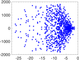
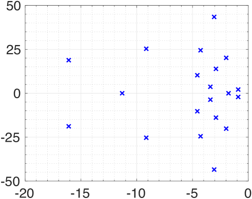
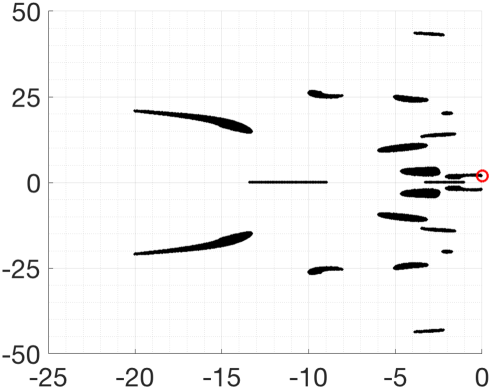
on such random examples. The spectrum of a typical of size generated in this way is depicted in Figure 1 on the left.
 |
 |
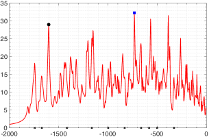
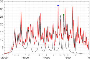
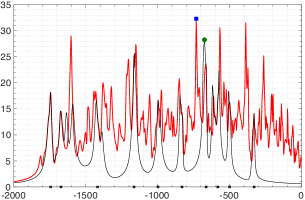
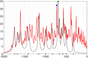
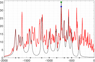
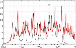
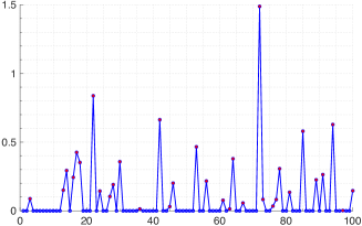
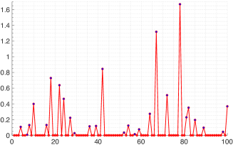
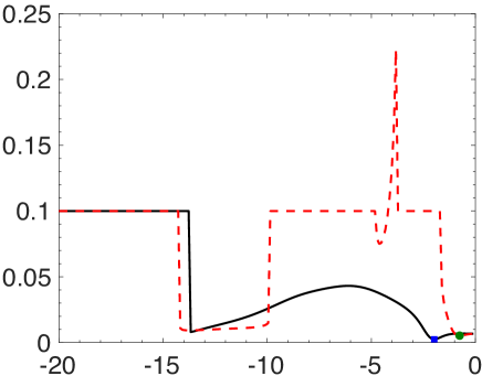
The progress of Algorithm 2, as well as Algorithm 1 in [2], to compute for this example is presented in Figure 2, which includes on the top left a plot of for along with the converged maximizers by the respective Algorithms. Algorithm 2 converges to the global maximizer with , while Algorithm 1 in [2] converges to the local maximizer with . The globally optimal peak and the locally optimal peak are marked in the plot with a square and a circle, respectively.
The remaining five plots in Figure 2 illustrate the progress of Algorithm 2. In each one of these plots, the black curve is a plot of the reduced function with respect to , and the circle marks the global maximizer of this reduced function. The top right shows the initial reduced function in black interpolating the full function at ten points, and the other four show the reduced function after iterations - from middle-left to bottom-right. Observe that, at every iteration, the refined reduced function interpolates the full function at the maximizer of the previous reduced function in addition to the earlier interpolation points. We also list the iterates of Algorithm 2 in Table 1 indicating a quick converge. The algorithm terminates after performing six subspace iterations.
The results of Algorithms 1 and 2 for the first random examples are presented in Tables 2 and 3, respectively. Results from [2, Algorithm 1] and the BB Algorithm [4] are also included in these tables for comparison purposes. For the computation of , the new structure-preserving Algorithm 1 and [2, Algorithm 1] perform equally well on these first examples. They both return the globally optimal solutions in out of examples, perform similar number of subspace iterations and require similar amount of cpu-time.
 |
 |
 |
 |
 |
 |
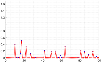
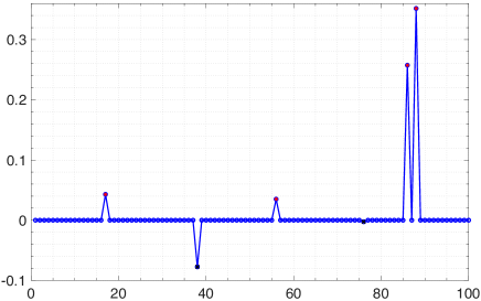
A more decisive conclusion can be drawn when we consider all of the random examples. The left-hand columns in Figure 3 depict the ratios , where are the globally maximal values of over returned by the BB algorithm and are the values returned by the subspace frameworks, specifically by Algorithm 1 on the top and by [2, Algorithm 1] at the bottom. The results by Algorithm 1 match with the ones by the BB algorithm times out of , while the results by Algorithm [2, Algorithm 1] match with the ones by the BB algorithm times out of . (In the examples where the results by the subspace frameworks differ from those by the BB algorithm, the subspace frameworks converge to local maximizers that are not global maximizers.)
On these random examples Algorithm 1 performs slightly fewer iterations, on average , whereas [2, Algorithm 1] on average performs iterations. On the other hand, the total run-time on average is better for [2, Algorithm 1] compared with Algorithm 1 here, vs . We observe this behavior on various other DH systems; Algorithm 1 seems to be more robust for the computation of in converging to the globally maximal value of compared with [2, Algorithm 1], however, this is at the expense of slightly more computation time.
On the other hand, for the computation of , Table 3 indicates that Algorithm 2 returns exactly the same globally maximal values (up to tolerances) as the BB algorithm for all of the first examples except one, whereas application of [2, Algorithm 1] results in locally maximal solutions that are not globally maximal times. Fewer number of subspace iterations in favor of Algorithm 2 are also apparent from the table. Once again, the plots of the ratios are shown in Figure 3 on the right-hand column for all examples with now representing the values returned by Algorithm 2 on the top and by [2, Algorithm 1] at the bottom. Algorithm 2 and [2, Algorithm 1] return locally optimal solutions that are not globally optimal and times, respectively. In this case the difference between the number of subspace iterations for these examples is more pronounced in favor of Algorithm 2; indeed the number of subspace iterations is on average for Algorithm 2 and and for [2, Algorithm 1]. This difference in the number of iterations is also reflected in the average run-times which are and for Algorithm 2 and [2, Algorithm 1], respectively.
| 10 | -600.705819 | 26.182525 |
|---|---|---|
| 11 | -674.769938 | 28.262865 |
| 12 | -697.139310 | 34.834307 |
| 13 | -731.573363 | 35.133647 |
| 14 | -731.942586 | 32.309246 |
| 15 | -731.977386 | 32.321399 |
| 16 | -731.977385 | 32.321399 |
| iterations | run-time | ||||||
|---|---|---|---|---|---|---|---|
| Ex. | Alg. 1 | [2, Alg. 1] | BB Alg. [4] | Alg. 1 | [2] | Alg. 1 | [2] |
| 1 | 32.559659 | 32.559659 | 32.559659 | 9 | 9 | 14 | 13 |
| 2 | 46.703932 | 46.703932 | 46.703932 | 15 | 12 | 16 | 12.4 |
| 3 | 26.227029 | 24.023572 | 26.227029 | 7 | 12 | 12.9 | 15.1 |
| 4 | 62.748090 | 108.030409 | 108.030409 | 17 | 41 | 17.8 | 27.2 |
| 5 | 35.974956 | 35.974957 | 35.974956 | 9 | 14 | 13.4 | 13.9 |
| 6 | 53.522033 | 53.522033 | 53.522033 | 6 | 3 | 11.4 | 10.2 |
| 7 | 31.739000 | 31.739000 | 31.739000 | 4 | 12 | 11.6 | 13.8 |
| 8 | 76.958658 | 76.958658 | 76.958658 | 35 | 8 | 43.2 | 11 |
| 9 | 37.007241 | 37.007241 | 37.007241 | 6 | 2 | 13 | 11.5 |
| 10 | 155.642871 | 155.642871 | 155.642871 | 2 | 2 | 8.6 | 8.5 |
| iterations | run-time | ||||||
|---|---|---|---|---|---|---|---|
| Alg. 1 | [2, Alg. 1] | BB Alg. [4] | Alg. 1 | [2] | Alg. 1 | [2] | |
| 1 | 9.809182 | 9.809182 | 9.809182 | 3 | 26 | 11.1 | 19.5 |
| 2 | 22.386670 | 22.386670 | 22.386670 | 5 | 26 | 10.2 | 18.1 |
| 3 | 8.364927 | 8.364927 | 8.364927 | 3 | 8 | 11 | 13.3 |
| 4 | 32.321399 | 29.028197 | 32.321399 | 6 | 37 | 10.5 | 25.2 |
| 5 | 15.071678 | 15.071678 | 15.071678 | 7 | 15 | 12.7 | 14 |
| 6 | 21.641484 | 21.641484 | 21.641484 | 4 | 8 | 10.2 | 11.6 |
| 7 | 12.858494 | 12.763161 | 12.858494 | 6 | 4 | 11.8 | 11.2 |
| 8 | 31.901305 | 27.996873 | 31.901305 | 8 | 12 | 11.5 | 12.5 |
| 9 | 9.228945 | 9.228945 | 9.228945 | 3 | 8 | 11.3 | 13 |
| 10 | 47.697528 | 47.697528 | 71.534252 | 10 | 8 | 11.8 | 10.2 |
 |
 |
 |
 |
Sparse Random Examples. The sparse matrices are constrained to be banded with bandwidth . The matrix is generated as in the dense family randomly using the randn command, but the entries that fall outside of the bandwidth are set equal to zero. The matrix is created using the commands
>> A = sprandn(n,n,1/n); >> Q = (A + A’)/2,
followed by setting the entries outside the bandwidth again to zero. Finally, the following commands ensure that .
>> mineig = eigs(Q,1,’smallestreal’);
>> if (mineig<10^-4) Q=Q+(-mineig+5*rand)*speye(n); end
To form , first a diagonal matrix of random rank not exceeding is generated by the commands
>> p = round(500*rand);   D = sparse(5000,5000);   h = n/p;
>> for j=1:p  k = floor(j*h); D(k,k) = 5*rand;  end
Then we set R = sparse(X’*D*X) for a square random matrix with bandwidth . The matrices , are random, and of size , , respectively. The spectrum of a typical such sparse matrix is displayed in Figure 1 on the right-hand side.
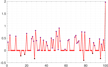
We again apply Algorithms 1 and 2 to such random sparse examples. Since the matrices are too large to apply the BB algorithm, we compare the structure-preserving algorithms directly with the unstructured algorithm [2, Algorithm 1]. The retrieved estimates of for and are compared on the top and at the bottom, respectively, in Figure 4. Specifically, the ratio is plotted for each random example with denoting the estimate by the unstructured algorithm [2, Algorithm 1], and denoting the estimate by the structured algorithm, i.e., Algorithm 1 for the top plot, Algorithm 2 for the bottom plot. According to the top plot, which concerns the computation of , the two algorithms return exactly the same results (up to tolerances) for all but examples; the structured algorithm returns better estimates for of these examples, while the unstructured algorithm returns better estimates for the other two. The structured algorithm appears to be even more robust for the computation of in terms of avoiding locally optimal solutions away from global solutions; as displayed at the bottom, the structured algorithm returns a better estimate for of the examples, the unstructured algorithm returns the better estimate for examples, and the results match exactly up to the tolerances for the remaining examples.
The structured algorithms perform typically fewer iterations as compared to the unstructured algorithm. Indeed the average value of the number of subspace iterations performed on these examples is for the structured and for the unstructured algorithm for the computation of , while these average values are and for the computation of . On the other hand, the unstructured algorithm is slightly superior when run-times are taken into account. The average run-times are for the structured and for the unstructured algorithm for the computation of , whereas these figures are and for the computation of .
We also list the computed maximal values of and over for the first of these sparse examples in Tables 4 and 5. Included in these tables are also the number of subspace iterations, as well as the run-time required by the structured and the unstructured algorithm.
 |
 |
| iterations | run-time | |||||
|---|---|---|---|---|---|---|
| Alg. 1 | [2, Alg. 1] | Alg. 1 | [2] | Alg. 1 | [2] | |
| 1 | 2 | 3 | 10.7 | 10.1 | ||
| 2 | 6 | 11 | 12.3 | 11.9 | ||
| 3 | 4 | 3 | 11.2 | 10.6 | ||
| 4 | 5 | 16 | 13.2 | 14 | ||
| 5 | 26 | 46 | 30.3 | 31.4 | ||
| 6 | 1 | 1 | 6.6 | 6.1 | ||
| 7 | 1 | 1 | 9.7 | 9.6 | ||
| 8 | 1 | 2 | 9.1 | 9 | ||
| 9 | 2 | 3 | 12.3 | 12.1 | ||
| 10 | 2 | 10 | 10.9 | 11.3 | ||
| iterations | run-time | |||||
|---|---|---|---|---|---|---|
| Alg. 2 | [2, Alg. 1] | Alg. 2 | [2] | Alg. 2 | [2] | |
| 1 | 15 | 39 | 18.3 | 26.7 | ||
| 2 | 2 | 13 | 11.1 | 12.7 | ||
| 3 | 31 | 11 | 46.1 | 11.8 | ||
| 4 | 5 | 17 | 13.1 | 14.6 | ||
| 5 | 3 | 9 | 11.3 | 11.4 | ||
| 6 | 1 | 1 | 6.4 | 6.1 | ||
| 7 | 4 | 12 | 10.6 | 11.1 | ||
| 8 | 8 | 9 | 11.8 | 10 | ||
| 9 | 13 | 4 | 17.9 | 12.1 | ||
| 10 | 3 | 7 | 10.8 | 10.6 | ||
4.3.3 The FE model of a Disk Brake
The only large-scale computation required by Algorithm 1 is the solution of the linear systems
| (4.25) |
at a given in lines 2 and 6, where . For the DH system resulting from a FE model of a disk brake in (1.6) and (1.7), the mass matrix and the stiffness matrix are available from the FE modeling. In other words, we have the sparse matrix , but not , which turns out to be dense. Trying to invert and/or solve a linear system with the coefficient matrix is computationally very expensive and would require full matrix storage.
This difficulty can be avoided by exploiting that
Hence, to compute as in (4.25), we proceed as follows.
-
(1)
We first solve for , and set .
-
(2)
Then we solve for , and set .
A second observation that further speeds up the computation is the particular structure of the coefficient matrix with . Setting , we have
Hence, to solve , for a given and the unknown with having all equal number of rows, we perform a column block permutation and then eliminate the lower left block to obtain
which in turn yields
At every subspace iteration, the highest costs arise from the computation of the factorizations of the sparse matrices and .
The main cost for Algorithm 2 is the solution of the linear systems
at a given . This can be treated similarly by exploiting that
We have applied Algorithm 1 to compute the unstructured stability radius for the DH system of the form (1.6), (1.7) resulting from the FE brake model with , where so that .
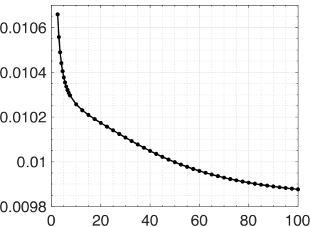
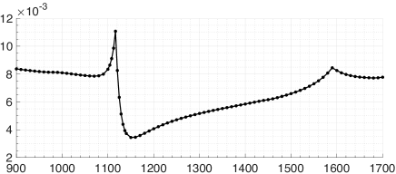
The plot of the computed vs the rotation speed is presented in Figure 5 at lower frequencies (i.e., ) on the top, and at higher frequencies (i.e., ) at the bottom. For smaller frequencies, the stability radius initially decreases with respect to , but around the stability radius suddenly increases. The non-smooth nature of the stability radius with respect to is apparent from the figure. One should note, in particular, the sharp turns near and ; this non-smoothness is due to the fact that has multiple global maximizers. This means that two distinct points on the imaginary axis can be attained with perturbations of minimal norm.
The computed values of are listed in Table 6 for some values of . In this table, for each , the value , where the singular value function is maximized globally is displayed, the number of subspace iterations, the run-time (in ) and the subspace dimension at termination are included as well. In all cases, or subspace iterations are sufficient to achieve the prescribed accuracy tolerance. This leads to considerably smaller reduced systems of size or compared with the original problem of size . The value maximizing differs substantially, depending on whether the frequency is small or large.
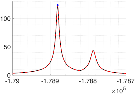
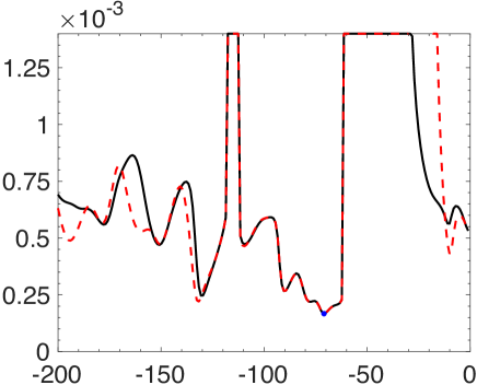
The resulting reduced problems at termination capture the full problem remarkably well around the global maximizer. This is depicted in Figure 6, where, for , the singular value function for the full problem (solid curve) and for the reduced problem at termination (dashed curve) are plotted near the global maximizer . It is fairly difficult to distinguish these two curves from each other.
| iterations | run-time | dimension | |||
|---|---|---|---|---|---|
| 2.5 | 0.01066 | 2 | 22.0 | 72 | |
| 5 | 0.01038 | 2 | 21.7 | 72 | |
| 10 | 0.01026 | 3 | 24.9 | 78 | |
| 50 | 0.00999 | 2 | 22.0 | 72 | |
| 100 | 0.00988 | 2 | 22.1 | 72 | |
| 1000 | 0.00809 | 2 | 21.4 | 72 | |
| 1050 | 0.00789 | 2 | 21.8 | 72 | |
| 1100 | 0.00834 | 3 | 24.8 | 78 | |
| 1116 | 0.01091 | 3 | 25.6 | 78 | |
| 1150 | 0.00344 | 2 | 21.5 | 72 | |
| 1200 | 0.00407 | 2 | 21.8 | 72 | |
| 1250 | 0.00471 | 2 | 21.8 | 72 | |
| 1300 | 0.00516 | 2 | 21.2 | 72 |
 |
 |
 |
5 Computation of the Structured Stability Radius
In the last section we have studied stability radii for dissipative Hamiltonian systems where the restriction matrices, however, allowed unstructured perturbations in the system coefficients. In this section we put additional constraints on the perturbations, in particular we require that the perturbations are structured themselves. We discuss only perturbations in the dissipation matrix, since this is usually the most uncertain part of the system, due to the fact that modeling damping or friction very exactly is usually extremely difficult. We deal with the computation of defined as in (2.4). We first describe a numerical technique for small-scale problems in Section 5.1 and then develop a subspace framework that converges superlinearly with respect to the subspace dimension in Section 5.2. Both techniques use the eigenvalue optimization characterization of in Theorem 3.2.
5.1 Small-Scale Problems
5.1.1 Inner Maximization Problems
The eigenvalue optimization characterization of is a min-max problem, where the inner maximization problem is concave, indeed it can alternatively be expressed as a semi-definite program (SDP). Formally, for a given , and representing the Hermitian matrices defined in Theorem 3.2, we have
| (5.1) |
where the characterization in the second line is a linear convex SDP. Here is related to a structured backward error for the eigenvalue , specifically it corresponds to the square of the distance (see [15, Definition 3.2 and Theorem 4.9])
| (5.2) |
We have that is finite if and only if the suprema in (5.1) are attained, which happens if and only if is indefinite, i.e., has both negative and positive eigenvalues.
The most widely used techniques to solve a linear convex SDP are different forms of interior-point methods. Implementations of some of these interior-point methods are made available through the package cvx [8, 9]. Hence, one option is to use cvx to compute directly. An alternative, and also theoretically well understood approach, is to employ the software package eigopt [16] for the eigenvalue optimization problem in the first characterization in (5.1). This second approach forms piece-wise quadratic functions that lie globally above the eigenvalue function, and maximizes these piece-wise quadratic functions instead of the eigenvalue function. Each piece-wise quadratic function is defined as the minimum of several other quadratic functions, all of which have the same curvature (which must be a global upper bound on the second derivative of the eigenvalue function at all points where the eigenvalue function is differentiable). Any slightly positive real number for the curvature serves the purpose (e.g., ), since the smallest eigenvalue function in (5.1) is a concave function of .
In our experience, eigopt performs the computation of significantly faster than cvx. The only downside is that an interval containing the optimal for (5.1) must be supplied to eigopt, whereas such an interval is not needed by cvx.
5.1.2 Outer Minimization Problems
The minimum of with respect to yields the distance , and the minimizing yields the point that first becomes an eigenvalue on the imaginary axis under the smallest perturbation possible. This is a non-convex optimization problem, indeed the objective may even blow up at some .
We again resort to eigopt for the minimization of . For the sake of completeness, a formal description is provided in Algorithm 3 below, where we use the abbreviations
Introducing , the algorithm approximates the smallest eigenvalue function
with the piece-wise quadratic function
at iteration . It computes the global minimizer of , and refines the piece-wise quadratic function with the addition of one more quadratic piece, namely . Here, is supposed to be a lower bound for the second derivative for all sufficiently close to the global minimizer of . In theory, it can be shown that for all small enough, every convergent subsequence of the sequence converges to a global minimizer of .
At step of the algorithm and its derivative need to be computed at . We rely on one of the two approaches (cvx or eigopt) described in Section 5.1.1 for the computation of , and employ a finite difference formula to approximate its derivative.
5.2 Large-Scale Problems
The characterization via eigenvalue optimization in Theorem 3.2 is in terms of the matrix-valued functions , which are of small size provided that has few columns. The large-scale nature of this characterization is hidden in the matrix-valued function defined in Theorem 3.2. Note that, in particular, both and are defined in terms of . This is also reflected in Algorithm 3 when are large; at iteration of the algorithm, the matrices , need to be formed for the computation of , which in turn requires the solution of the linear system .
To cope with the large-scale setting, we benefit from structure preserving two-sided projections similar to those described in Section 4.2. In particular, for a given subspace and a matrix whose columns form an orthonormal basis for , we set
| (5.3) |
Furthermore, we define the projected matrices
| (5.4) |
Recall also the identities
| (5.5) |
the latter of which means that is an oblique projector onto .
Although these identities are still available, however, we no longer have a tool such as Theorem 4.1 that we could depend on to establish interpolation results. This is because there is no apparent transfer function, as there is indeed no apparent linear port-Hamiltonian system that can be tied to the eigenvalue optimization characterization. But the following simple observation turns out to be very useful.
Lemma 5.1.
Our reduced problems are expressed in terms of the reduced versions of , , and defined via
with denoting a lower triangular Cholesky factor of
and with
Note that to ensure the uniqueness of and , we define them as the Cholesky factors of and with real and positive entries along the diagonal. Our goal is to come up with reduced counterparts of , that Hermite-interpolate the full functions at prescribed points. For a given subspace , a matrix whose columns form an orthonormal basis for , and for as in (5.3), we introduce
Recall that , and a similar relation holds for the reduced problems, i.e., .
We start our analysis by establishing that the quantities , are independent of the choice of basis for the subspace . For this proof we introduce the notation , to emphasize the particular choices of basis for the subspaces used in the definitions of . Similarly, we indicate the spaces and the bases with the help of the notations , , , and .
Lemma 5.2.
Let the columns of and form orthonormal bases for the subspace , and let , . Then
for all .
Proof.
It suffices to prove , the other equality follows from this equality immediately. Since the columns of and form bases for the same space, there exists a unitary matrix such that . Furthermore, by definition,
The assertion then follows from the following set of equivalences:
∎
In the following we will develop a subspace framework including an Hermite interpolation property for DH systems. For this we first show an auxiliary interpolation result for , the matrix through which are defined.
Theorem 5.3.
Consider a DH model (1.1) and a reduced model with coefficients as in (5.4), and let and . For a given such that and are invertible, the following assertions hold:
-
(i)
If , then .
-
(ii)
Additionally, if and the orthonormal basis for is such that where the columns of form an orthonormal basis for , then .
Proof.
(i) If then, since is a projector onto , we obtain
To show that , let , and be such that . (There exists a unique with this property, because .) Then implies that , and thus . Hence, by Lemma 5.1 we see that , implying that
as asserted.
(ii) Following the steps at the beginning of the proof of part (i), we have
To show that , we exploit that
| (5.6) |
Now define and such that (once again such a exists uniquely, because ) so that . Then and hence , where is the matrix consisting of the first columns of the identity matrix with . This implies that , so the following can be deduced about the term inside the first parenthesis on the right-hand side of (5.6):
As for the term inside the second parenthesis on the right-hand side of (5.6), we make use of the following observation:
| (5.7) |
where the last equality follows, since the columns of form an orthonormal basis for . Putting these observations together in (5.6), we obtain
where in the third equality we exploit (5.7), and in the fourth equality we employ that which is proven in part (i). ∎
After these preparations we can prove our main interpolation result.
Theorem 5.4.
Consider a DH model (1.1) and a reduced model with coefficients as in (5.4), and let and . Suppose that the subspace is such that
| (5.8) |
and is defined as in (5.3) in terms of a matrix whose columns form an orthonormal basis for .
-
(i)
The quantity is finite if and only if is finite. If is finite, then
(5.9) -
(ii)
Moreover, if and are differentiable at , then we have
(5.10)
Proof.
Without loss of generality, we may assume that the matrix is such that with the columns of forming an orthonormal basis for . It suffices to prove the claims for this particular choice of orthonormal basis, because it is established in Lemma 5.2 that the function , hence its derivative, are independent of the choice of as long as its columns form an orthonormal basis for .
(i) By the definitions of , and part (i) of Theorem 5.3, we have
This also implies that due to the uniqueness of the Cholesky factors of , . Therefore,
Furthermore,
and
Since , it follows that is finite if and only if is finite. Additionally, if is finite, then
completing the proof of (5.9).
(ii) Now let us suppose that and are differentiable at . To prove the interpolation property in the derivatives, we benefit from the analytical expressions [14]
| (5.11) |
where
and is a unit eigenvector corresponding to . Thus, it suffices to prove that and in order to show (5.10). It follows from parts (i) and (ii) of Theorem 5.3 that
Now let us determine the derivatives of the Cholesky factors, which at a given satisfy
Differentiating these two equations, and setting the derivatives equal to each other at yield
where we have used that as established in part (i). Thus, both and are lower triangular solutions of the matrix equation
This linear matrix equation has a unique lower triangular solution, so . Now, by the definitions of , we have
Differentiating this equation at yields
Using that , , and , we deduce that . Next we focus on the derivatives . In particular, we use that
Differentiating both sides of the last equation at gives rise to
which in turn implies that
Once again exploiting that , , as well as in the last equation, we obtain which implies that
and the proof of (5.10) is complete. ∎
-
Remark
The function is differentiable at whenever is finite (equivalently is indefinite), is simple where , and the global minimum of over is attained at a unique . These conditions guarantee also the differentiability of at provided the subspace inclusion in (5.8) holds. This latter differentiability property is due to and from part (i) of Theorem 5.4.
Additionally, when the concave function attains its maximum, the maximizer is nearly always unique. The function is the minimum of real analytic functions [13, 19] each corresponding to an eigenvalue of . If does not have a unique maximizer, then at least one of these real analytic functions must be constant and equal to everywhere. Thus, a simple sufficient condition that ensures the uniqueness of the maximizer is that has full rank, in which case all eigenvalues of blow up (either to or ) as implying that each of the real analytic functions is non-constant.
5.2.1 The Subspace Framework for
The Hermite interpolation result of Theorem 5.4 immediately suggests the subspace framework in Algorithm 4 for the computation of . This resembles the structure preserving subspace framework to compute the unstructured stability radii , in particular, in the way the subspaces are built. At every iteration, a reduced problem is solved using the ideas in Section 5.1 and employing Algorithm 3. Letting be the global minimizer of the reduced problem, the subspaces are expanded so that the original function is Hermite interpolated by its reduced counter-part at .
Assuming that the sequence converges to a minimizer of the function such that is indefinite with full rank and is simple where , it can be shown that the sequence converges at a super-linear rate. Here the analysis in [3] applies. The conditions that is indefinite with full rank, is simple, and the interpolation properties , ensure that the full function , as well as the reduced function for all large are differentiable at all in a ball centered at and of radius . This differentiability property is essential for the applicability of the rate-of-convergence analysis in [3].
5.3 Numerical Experiments
In this section we present several numerical tests for Algorithms 3 and 4, on synthetic examples and the FE model of the disk brake. The test set-up is similar to the one for the unstructured case in Section 4.3. In particular, for Algorithm 4, we use the same stopping criteria with the same parameters, but now in terms of , so we terminate when holds, or when one of the other two conditions stated in Section 4.3.1 holds. The initial subspaces are also chosen as described in that section.
5.3.1 Synthetic Examples
Small Scale Examples. We first present numerical results for a small dense random example, where and . These matrices are generated by means of the MATLAB commands employed for the generation of the dense family in Section 4.3.2; only here the matrices are instead of and is of rank .
The spectrum of is depicted on the top in Figure 7. Application of Algorithm 3 to this example yields , and the point that is first reached on the imaginary axis under the smallest perturbation is , i.e., is minimized at . At the bottom of Figure 7, the spectra of matrices of the form are plotted for randomly chosen Hermitian such that . One can notice that some of the eigenvalues (nearly) touch the imaginary axis at marked with a circle.
 |
 |
The subspace framework for this example is illustrated in Figure 8, where the solid, dashed curves correspond to the plots of the full function , the reduced function , respectively, and the circle represents the minimizer of . On the top row, the framework is initiated with two interpolation points at 0 and near -20; the dashed curve interpolates the solid curve at these points. Then the subspaces are expanded so that the Hermite interpolation property is also satisfied at the minimizer of the dashed curve on the top, leading to the dashed curve at the bottom, which has nearly the same global minimizer as the solid curve. Note that starting from near -14 and for smaller values, the matrix turns out to be definite for this example, meaning for such values the point is not attainable as an eigenvalue with Hermitian perturbations. In practice, we set the objective to be minimized at such a value considerably larger than the minimal value of the objective, which in this example is 0.1.
Large Examples. The remaining synthetic examples are with larger random matrices. We created three sets of matrices using the commands at the beginning of Section 4.3.2 for the generation of the dense family. Each of the three sets consists of four quadruples , with the same , specifically for the first, second, third set. The results obtained by applications of Algorithm 4 to compute are reported in Tables 7, 8, 9 for these sets, respectively.
For the first family with , the subspace framework, i.e., Algorithm 4 already needs less computing time than Algorithm 3 except for the last example where quite a few additional subspace iterations have been performed. On this family, the direct application of Algorithm 3 and the subspace framework return exactly the same values for .
For bigger systems Algorithm 3 becomes too computationally expensive, so we do not report results here for the larger dimensions. A remarkable fact we have observed is that the number of subspace iterations to reach the prescribed accuracy is usually small and seems independent of . By the definitions of the structured and unstructured radii, we must have , and the presented radii in the tables are in harmony with this.
All of these examples involve optimization of highly non-convex and non-smooth functions. Figure 9 depicts as a function of with the solid curve for the first example in the first family with . The same figure also depicts the reduced function with the dashed curve for the same example at termination after 7 subspace iterations. Even though the reduced function represented by the dashed curve in this plot is defined for projected matrices onto dimensional subspaces, it captures the original function remarkably well near the global minimizer .
 |
 |
 |
| iterations | run-time | |||||
|---|---|---|---|---|---|---|
| Alg. 3 | Alg. 4 | Alg. 1 | Alg. 4 | Alg. 3 | Alg. 4 | |
| 1 | 0.0129 | 0.0129 | 0.0113 | 7 | 99.2 | 66.2 |
| 2 | 0.0101 | 0.0101 | 0.0101 | 1 | 66.5 | 7.1 |
| 3 | 0.0141 | 0.0141 | 0.0128 | 5 | 128.5 | 72.5 |
| 4 | 0.0096 | 0.0096 | 0.0072 | 20 | 121.2 | 247.2 |
| iterations | run-time | |||
|---|---|---|---|---|
| Alg. 4 | Alg. 1 | Alg. 4 | Alg. 4 | |
| 1 | 0.0102 | 0.0061 | 6 | 149.1 |
| 2 | 0.0040 | 0.0012 | 1 | 17.1 |
| 3 | 0.0125 | 0.0109 | 6 | 175.9 |
| 4 | 0.0101 | 0.0100 | 3 | 126.7 |
| iterations | run-time | |||
|---|---|---|---|---|
| Alg. 4 | Alg. 1 | Alg. 4 | Alg. 4 | |
| 1 | 0.0090 | 0.0087 | 2 | 282.6 |
| 2 | 0.0084 | 0.0068 | 3 | 319.3 |
| 3 | 0.0104 | 0.0086 | 2 | 333.1 |
| 4 | 0.0040 | 0.0007 | 46 | 786.5 |
5.3.2 FE Model of a Disk Brake
We also applied our implementation of Algorithm 4 to the FE model of the disk brake described in Section 4.3.3 which is of the form (1.6), (1.7) with , and .
The computed value of the structured radius along with the computed global minimizer of , as well as the number of subspace iterations, run-time (in ) and the subspace dimension at termination are listed in Table 10 for various values of . It is worth comparing the computed values of in this table with those for the unstructured stability radius listed in Table 6. The computed structured and the unstructured stability radii are close, though the structured stability radii are slightly larger as expected in theory.
| iterations | run-time | dimension | |||
|---|---|---|---|---|---|
| 2.5 | 0.01067 | 2 | 145.8 | 72 | |
| 5 | 0.01038 | 2 | 133.5 | 72 | |
| 10 | 0.01026 | 2 | 132.0 | 72 | |
| 50 | 0.01000 | 2 | 132.5 | 72 | |
| 100 | 0.00988 | 1 | 94.4 | 66 | |
| 1000 | 0.00810 | 2 | 127.7 | 72 | |
| 1050 | 0.00794 | 2 | 126.4 | 72 | |
| 1100 | 0.00835 | 3 | 171.2 | 78 | |
| 1116 | 0.01092 | 2 | 127.4 | 72 | |
| 1150 | 0.00346 | 2 | 124.3 | 72 | |
| 1200 | 0.00408 | 2 | 121.2 | 72 | |
| 1250 | 0.00472 | 2 | 119.1 | 72 | |
| 1300 | 0.00517 | 2 | 117.1 | 72 |
6 Concluding Remarks
We have proposed subspace frameworks to compute the stability radii for large scale dissipative Hamiltonian systems. The frameworks operate on the eigenvalue optimization characterizations of the stability radii derived in [15]. At every iteration, we apply DH structure preserving Petrov-Galerkin projections to small subspaces. This leads to the computation of the corresponding stability radii for the reduced system. We expand the subspaces used in the Petrov-Galerkin projections so that Hermite-interpolation properties between the objective eigenvalue function of the full and the reduced problems are attained at the optimizer of the reduced problem. This strategy results in super-linear convergence with respect to the subspace dimensions. We have illustrated that the frameworks work well in practice on several synthetic examples, and a FE model of a disk brake.
Matlab implementations of the proposed algorithms and subspace frameworks are made publicly available on the web***http://home.ku.edu.tr/~emengi/software/DH-stabradii.html. Some of the data (including the one associated with the disk brake example) used in the numerical experiments are also available on the same website.
One difficulty is that the proposed frameworks converge only locally. As a remedy for this, we have initiated the subspaces to attain Hermite interpolation at several points on the imaginary axis between the full and initial reduced problems. One potential strategy that is currently investigated is to employ equally spaced interpolation points. Another potential strategy finds the poles closest to these equally spaced points, then employs the imaginary parts of the poles as the initial interpolation points.
Another research direction that is currently investigated is the maximization of the stability radii, when depend on parameters in a given parameter set. As an example, for the dissipative Hamiltonian system arising from the FE model of a disk brake, even in the simple setting considered here, depend on the rotation speed .
References
- [1] A. Akay. Acoustics of friction. J. Acoust. Soc. Am., 111(4):1525–1548, 2002.
- [2] A. Aliyev, P. Benner, E. Mengi, P. Schwerdtner, and M. Voigt. Large-scale computation of -norms by a greedy subspace method. SIAM J. Matrix Anal. Appl., 38(4):1496–1516, 2017.
- [3] A. Aliyev, P. Benner, E. Mengi, and M. Voigt. A subspace framework for -norm minimization. Technical report, 2018. In Preparation.
- [4] S. Boyd and V. Balakrishnan. A regularity result for the singular values of a transfer matrix and a quadratically convergent algorithm for computing its -norm. Systems Control Lett., 15(1):1–7, 1990.
- [5] N. A. Bruinsma and M. Steinbuch. A fast algorithm to compute the -norm of a transfer function matrix. Systems Control Lett., 14(4):287–293, 1990.
- [6] K. Gallivan, A. Vandendorpe, and P. Van Dooren. Model reduction of MIMO systems via tangential interpolation. SIAM J. Matrix Anal. Appl., 26(2):328–349, 2005.
- [7] N. Gräbner, V. Mehrmann, S. Quraishi, C. Schröder, and U. von Wagner. Numerical methods for parametric model reduction in the simulation of disc brake squeal. Z. Angew. Math. Mech., 96:1388–1405, 2016.
- [8] M. Grant and S. Boyd. Graph implementations for nonsmooth convex programs. In V. Blondel, S. Boyd, and H. Kimura, editors, Recent Advances in Learning and Control, Lecture Notes in Control and Information Sciences, pages 95–110. Springer-Verlag Limited, 2008. http://stanford.edu/~boyd/graph_dcp.html.
- [9] M. Grant and S. Boyd. CVX: Matlab software for disciplined convex programming, version 2.1. http://cvxr.com/cvx, March 2014.
- [10] S. Gugercin, R. V. Polyuga, C. Beattie, and A. J. van der Schaft. Structure-preserving tangential interpolation for model reduction of port-Hamiltonian systems. Automatica, 48(9):1963–1974, 2012.
- [11] S. Gugercin, R. V. Polyuga, C. A. Beattie, and A. J. van der Schaft. Interpolation-based model reduction for port-Hamiltonian systems. In Decision and Control, 2009 held jointly with the 2009 28th Chinese Control Conference. CDC/CCC 2009. Proceedings of the 48th IEEE Conference on, pages 5362–5369, Dec 2009.
- [12] B. Jacob and H. Zwart. Linear port-Hamiltonian systems on infinite-dimensional spaces. Operator Theory: Advances and Applications, 223. Birkhäuser/Springer Basel AG, Basel CH, 2012.
- [13] T. Kato. Perturbation Theory for Linear Operators. Springer-Verlag, Berlin Heidelberg, 1995.
- [14] P. Lancaster. On eigenvalues of matrices dependent on a parameter. Numer. Math., 6:377–387, 1964.
- [15] C. Mehl, V. Mehrmann, and P. Sharma. Stability radii for linear Hamiltonian systems with dissipation under structure-preserving perturbations. SIAM J. Matrix Anal. Appl., 37(4):1625–1654, 2016.
- [16] E. Mengi, E. A. Yildirim, and M. Kiliç. Numerical optimization of eigenvalues of Hermitian matrix functions. SIAM J. Matrix Anal. Appl., 35(2):699–724, 2014.
- [17] R. V. Polyuga and A. J. van der Schaft. Moment matching for linear port-Hamiltonian systems. In Control Conference (ECC), 2009 European, pages 4715–4720, Aug 2009.
- [18] R. V. Polyuga and A. J. van der Schaft. Structure preserving moment matching for port-Hamiltonian systems: Arnoldi and Lanczos. IEEE Trans. Autom. Cont., 56(6):1458–1462, June 2011.
- [19] F. Rellich. Perturbation Theory of Eigenvalue Problems. Notes on Mathematics and its Applications. Gordon and Breach, New York, NY, USA, 1969.
- [20] A. J. van der Schaft and D. Jeltsema. Port-Hamiltonian systems theory: An introductory overview. Foundations and Trends in Systems and Control, 1(2-3):173–378, 2014.
- [21] A. J. van der Schaft and R. V. Polyuga. Structure-preserving model reduction of complex physical systems. In Decision and Control, 2009 held jointly with the 2009 28th Chinese Control Conference. CDC/CCC 2009. Proceedings of the 48th IEEE Conference on, pages 4322–4327, Dec 2009.
- [22] Y. Wu, B. Hamroun, Y. Le Gorrec, and B. Maschke. Structure preserving reduction of port Hamiltonian system using a modified lqg method. In Control Conference (CCC), 2014 33rd Chinese, pages 3528–3533, July 2014.