The Missing Satellite Problem Outside of the Local Group
I – Pilot Observation

Abstract

We present results from a pilot observation of nearby ($\sim 20$ Mpc) galaxies with mass similar to that of the Milky Way (MW) to address the missing satellite problem. This is the first paper from an on-going project to address the problem with a statistical sample of galaxies outside of the Local Group (LG) without employing an assumption that the LG is a typical halo in the Universe. Thanks to the close distances of our targets, dwarf galaxies around them can be identified as extended, diffuse galaxies. By applying a surface brightness cut together with a careful visual screening to remove artifacts and background contamination, we construct a sample of dwarf galaxies. The luminosity function (LF) of one of the targets is broadly consistent with that of the MW, but the other has a more abundant dwarf population. Numerical simulations by Okamoto (2013) seem to overpredict the number of dwarfs on average, while more recent predictions from Copernicus Complexio are in a better agreement. In both observations and simulations, there is a large diversity in the LFs, demonstrating the importance of addressing the missing satellite problem with a statistically representative sample. We also characterize the projected spatial distributions of the satellites and do not observe strong evidence for alignments around the central galaxies. Based on this successful pilot observation, we are carrying out further observations to increase the sample of nearby galaxies, which we plan to report in our future paper.

1. Introduction

The $\Lambda$-dominated cold dark matter model ($\Lambda$CDM) is widely accepted as the standard cosmological model. It has passed many stringent observational tests on the large-scale matter distribution in the Universe, but it has a few possible flaws on small scales such as the cusp-core problem (McGaugh et al., 2001; Gilmore et al., 2007; Kuzio de Naray et al., 2008), too-big-to-fail problem (Boylan-Kolchin et al., 2011; Parry et al., 2012), missing satellite problem (Kauffmann et al., 1993; Klypin et al., 1999; Moore et al., 1999), and satellite alignment problem (Ibata et al., 2013; Pawlowski & Kroupa, 2013; Pawlowski et al., 2015). We do not have a satisfactory solution to these problems and they may urge us to adopt other models such as warm dark matter and self-interacting dark matter.

This is a pilot of a project that aims to address the missing satellite problem: more than an order of magnitude shortage of observed dwarf galaxies around the Milky Way (MW) and M31 compared to the number expected if every subhalo hosts a galaxy. The problem was first pointed out in 1999 based on (dark matter only) N-body simulations. Since then, there has been tremendous progress in hydro-dynamical simulations of galaxy formation in a cosmological context, and recent simulations show that, once baryonic effects such as star formation, SNe feedback, UV background due to cosmic reionization are incorporated, many subhalos do not actually host galaxies and the tension between the observed and expected numbers of dwarf galaxies is significantly reduced (e.g., Okamoto et al. 2010; Sawala et al. 2016a,b). While it is clear that baryonic astrophysics is a natural solution to the problem, all models are calibrated to reproduce the Local Group (LG). This is obviously not a fair test of the problem. Furthermore, different models that currently claim to solve the missing satellite problem use different assumptions about baryon physics. In order to distinguish between these solutions and see if any one of them can actually solve the problem, we need to test model predictions against a sample that has not been used in the calibration. Constraining the physics that governs the abundance of satellites is a necessary first step to addressing higher order problems like their density profiles (’cusp-core’), which in turn break degeneracies between baryonic astrophysics and alternate forms of dark matter.

There is some recent work in this direction. Geha et al. (2017) presented the first results from their spectroscopic campaign around galaxies at $20-40$ Mpc. They targeted galaxies from shallow SDSS data and constructed a luminosity function (LF) of the confirmed dwarf galaxies. We also have initiated a project to observationally test the missing satellite problem beyond the LG. This project is made possible with Hyper Suprime-Cam (HSC) mounted on the Subaru Telescope (Miyazaki et al., 2012). With its large light-collecting aperture over a wide area, we can now search for faint dwarf galaxies outside of the LG. This paper presents first results from our pilot observation. Unless otherwise stated, magnitudes are given in the AB system.

2. Data

2.1. Sample Selection

In order to achieve our goal, we target galaxies with MW-like mass. We assume that the halo mass of the MW is $1-2\times 10^{12}\rm M_{\odot}$ (see Bland-Hawthorn & Gerhard 2016 for a compilation). We construct a sample of galaxies with MW-like mass by first estimating stellar mass of nearby galaxies using photometry and distance measurements, translating it into halo mass using the abundance matching method, and then selecting galaxies with a halo mass similar to that of the MW. We detail each of these steps below.

It is not trivial to perform photometry of nearby galaxies because of their large extent on the sky. The Sloan Digital Sky Survey (SDSS; York et al. 2000) performed optical photometry of a large number of objects. But, even with the short exposure of SDSS, the cores of very nearby galaxies are often saturated, resulting in inaccurate photometry. We choose to use photometry from the Two-Micron All-Sky Survey (2MASS; Skrutskie et al. 2006). Because our first step is to estimate stellar mass, the near-IR photometry is good for its weaker sensitivities to star formation activities and dust than optical photometry. To be specific, we use the 2MASS Large Galaxy Atlas (Jarrett et al., 2003) as our primary source of photometry, supplemented with 2MASS extended source catalog (Jarrett et al., 2000). We correct for the (small) Galactic extinction in the near-IR photometry using the dust map from Schlegel et al. (1998). We then search for distance measurements of the objects in the 2MASS catalogs in the HyperLEDA database (Makarov et al., 2014), and objects with no reliable distance measurements are removed at this point.

We use the Bruzual & Charlot stellar population synthesis code (Bruzual & Charlot, 2003) in order to infer stellar mass from the photometry. We generate model templates and make a mapping between the $K$-band magnitude, $J-K$ color, and stellar mass assuming the exponentially decaying star formation histories, solar metallicity, and Chabrier IMF (Chabrier, 2003). We introduce the $J-K$ color here to correct for a small effect of the ongoing star-formation activities. To validate our stellar mass estimates, we compare our estimates with those from Spitzer Survey of Stellar Structure in Galaxies (S4G; Sheth et al. 2010), which performed a very careful analysis of stellar mass of nearby galaxies. We find that, for MW-like galaxies with a few – several $\times 10^{10}\rm M_{\odot}$, our stellar mass agrees well with S4G; the scatter between the two estimates is 0.15 dex with a small mean bias of $-0.1$ dex.

We then use the abundance matching result from Moster et al. (2010) to translate the stellar mass into halo mass. Given the scatter in the abundance matching and also uncertainty in our stellar mass estimates, we select objects with halo mass $0.5-4\times 10^{12}\rm M_{\odot}$. This is the primary constraint in our target selection. The corresponding stellar mass range is $1.2-8.0\times 10^{10}\rm M_{\odot}$. The stellar mass of the MW is estimated as $\sim 6\times 10^{10}\rm M_{\odot}$ (Licquia & Newman, 2015), which is indeed within the range of our selection. We note that the distances to the targets typically have a 10-15% uncertainty and it propagates to the mass and virial radius of the central galaxies. A change in the virial radius is the most concerning effect because it changes the radius within which we search for satellites. However, an angular scale change and a physical change in $r_{200}$ largely compensate each other, and the typical uncertainty in $r_{200}$ on the sky (i.e., apparent size of $r_{200}$) is only $\sim 5\%$ and is unlikely to significantly alter our conclusions.

In addition to mass, we apply the following conditions:

• Small ($<0.1$ mag) Galactic extinction in the $r$-band

• No bright ($\lesssim 6$ mag) stars within the field of view of HSC

• Virial radius ($r_{200}$) can be covered by a single HSC pointing

• Located at $\sim 20$ Mpc

• Declination above $-20$ deg

The first constraint is to stay away from the Galactic disk, where there are numerous stars, which make it difficult to look for diffuse extended sources. The 2nd is to avoid significant optical ghosts in the data. The 3rd constraint is simply for observing efficiency and is in fact coupled with the 4th constraint; galaxies too close to us have very large virial radii on the sky, which are difficult to cover even with HSC. On the other hand, targets should not be too far from us; as we discuss later, we apply a cut on surface brightness in order to select dwarf galaxies and this method becomes less effective at larger distances. Simulations performed in Section 3.4 suggests that a distance of $\sim 20$ Mpc is about the right distance for this work. The last constraint is simply a visibility constraint from Hawaii.

The MW has a massive companion galaxy (the Andromeda galaxy). We do not explicitly impose a constraint on the presence of a bright neighbor, but we do exclude galaxies in massive groups and clusters for the purpose of the paper. We compute a distance to the 2nd nearest neighbor within $\pm 1000\rm km\ s^{-1}$ in recession velocity for each object using the catalog constructed above. We exclude all galaxies that have the 2nd nearest neighbor within 1.5 deg. We visually inspect the remainder using images from the Digitized Sky Survey and exclude obvious groups. Our final targets are thus a mixture of isolated galaxies and galaxies in pairs. We do not apply any cut on colors of the targets. As a result, our targets include both early-type and late-type galaxies. Once we build a statistically large sample, we will be able to address the dependence of the abundance of dwarf galaxies on color and morphology of the central galaxies.

2.2. Observation and Data Processing

A pilot observation of this program was carried out in November 2014 with HSC in the $g$ and $i$-bands for $\sim 25$ minutes as summarized in Table 1. The observing conditions were photometric and the $g$-band data were taken under excellent seeing conditions, $\sim 0.5$ arcsec. The $i$-band data were obtained under less optimal conditions with seeing $\sim 1$ arcsec. Individual exposures were 4 and 2.5 min long in the $g$ and $i$-bands, respectively, and we applied a circular dither of 200 arcsec in between the exposures. In the pilot run, we observed 5 galaxies but some of them turned out to be problematic. We will elaborate on these problematic cases below. In this paper, we focus on two of the observed targets, N2950 and N3245. Their physical properties are summarized in Table 2.

The data was processed with hscPipe v5.4, a branch of Large Synoptic Survey Telescope pipeline (Ivezic et al., 2008; Axelrod et al., 2010; Jurić et al., 2015). The pipeline follows a standard procedure of CCD processing and the astrometric and photometric calibration was performed against data from the PanSTARRS1 (Schlafly et al., 2012; Tonry et al., 2012; Magnier et al., 2013) for each CCD separately. Because we are interested in extended objects, we used a relatively large grid of 512 pixel to estimate the sky background. The grid size is too small for the central galaxies, but they are not the main interest of this paper. Then, a joint calibration using multiple exposures of the same sources observed at different locations on the focal plane was performed to improve the relative astrometry and photometry. The fully calibrated CCD images were coadded to generate deep stacks. Our photometric zero-points are accurate to a few percent and astrometry to a few tens of milli-arcsec on the coadds (Aihara et al., 2018a).

Table 1Observational Data

Object	Filter	Seeing (arcsec)	Exposure
N2950	$g$	$0.48$	4 min $\times$ 6 shots
N2950	$i$	$1.18$	2.5 min $\times$ 10 shots
N3245	$g$	$0.51$	4 min $\times$ 6 shots
N3245	$i$	$0.89$	2.5 min $\times$ 7 shots

Table 2Physical Properties of the Targets

Object	Distance [Mpc]	stellar mass [$\rm M_{\odot}$]	halo mass [$\rm M_{\odot}$]	$r_{200}$ [kpc]	$r_{200}$ [arcmin]
N2950	$14.9^{a}$	$1.7\times 10^{10}$	$6.6\times 10^{11}$	176	40.5
N3245	$20.9^{a}$	$4.0\times 10^{10}$	$1.4\times 10^{12}$	227	37.3

3. Identification of Dwarf Satellite Galaxies

In this section, we describe how we identify the dwarf satellites. Because this work is based primarily on the photometric data, we do not have confirmation of membership from spectroscopy in most cases, aside from a few of the brighter dwarf galaxies, which have been observed in the SDSS. We make an attempt to construct a sample of dwarf galaxies as clean as possible by selecting dwarf galaxies by their low surface brightness, eliminating contamination by careful visual inspections, and then subtracting field contamination statistically using a control sample. This section describes each step of this procedure.

3.1. Object Detection and Masks Around Bright Stars

We detect objects using Source Extractor (Bertin & Arnouts, 1996). Due to the superb seeing, we use the $g$-band for the object detection. Detection parameters are tuned to detect diffuse sources and we adopt detect_minarea=100 and detect_thres=1$\sigma$. Obviously, these parameters are for extended sources and we intentionally miss a large number of faint compact sources. At a distance of 20 Mpc, 200pc ($\sim r_{eff}$ of $M_{V}=-10$ dwarfs) subtends 2 arcsec on the sky, and that is 12 pixel radius ($\sim 450$ pixels in area). We should be able to detect such faint dwarf galaxies with these parameters. One could explore a more sophisticated detection scheme such as the one adopted by Next Generation Virgo Cluster Survey (Ferrarese et al. 2012; MacArthur et al. in prep), but we choose to apply a simple object detection in this current paper and leave a more sophisticated detection algorithm for future work.

One of the major sources of false detections is outskirts of bright stars. A small statistical fluctuation at the outskirts causes Source Extractor to deblend that portion of the star from the main body, resulting in diffuse, faint objects. The easiest way to eliminate such artifacts is to aggressively mask regions around bright stars by identifying bright stars from their saturated cores in an automated way. The bleeding trails of saturated stars are also masked in the same way. Due to the large field of view of HSC, bright stars often cause optical ghosts, which are also detected as diffuse extended sources. We manually generate masks around optical ghosts. We further generate masks around bright, extended background galaxies as we detail in Section 3.3. All the objects within the masked area are removed from the catalog at this point. Due to the masks, we miss a fraction of the area inside the virial radius of a central galaxy. We statistically account for it when we construct the luminosity function in Section 4 using effective detection completeness estimates measured in Section 3.4.

3.2. Surface Brightness Cut

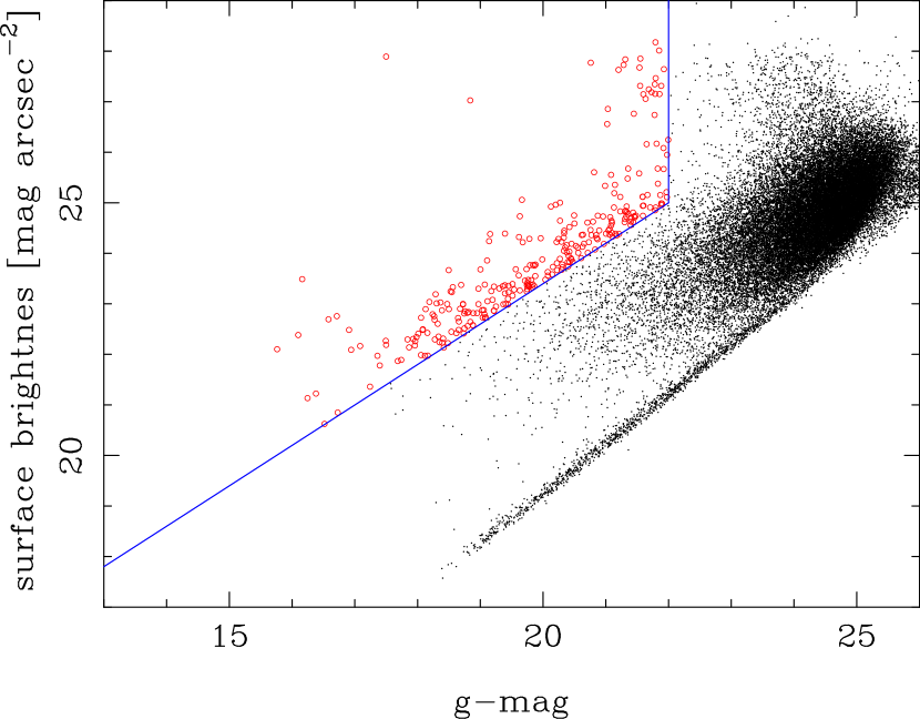
Figure 1.— Surface brightness plotted against magnitude. The dots are detected sources and the sources lined up in the bottom-right edge of the distribution are compact sources (stars). The solid lines indicate the surface brightness and magnitude cuts we apply and all objects that satisfy the cuts are indicated by the red circles. The surface brightness cut is tuned to select most of the MW dwarf galaxies when placed at the distance of $\sim 20$ Mpc, while keeping the contamination minimal (see Section 3.4 for details). This plot is for N2950, but N3245 looks identical. To improve the clarity, every 5 objects are plotted in the bottom-right, while all objects that satisfy the cut are plotted in the top-left.

In order to select dwarf galaxy candidates, we use the fact that the galaxies that we have observed are very nearby and hence dwarf galaxies around them are spatially extended, even though their physical sizes are as small as 200 pc. Most of the detected sources are located at much larger distances and they appear compact. This allows an efficient selection of dwarf galaxies with a surface brightness cut. We show in Fig. 1 our surface brightness cut. Note that the surface brightness is computed as the mean brightness within the effective radius. This cut is carefully set to include the majority of dwarf galaxies around the MW and Andromeda galaxies when placed at the distance of $\sim 20$ Mpc (see Section 3.4). In addition to the surface brightness cut, we also apply an apparent magnitude cut at $m_{g}<22$, which roughly corresponds to $M_{g}\sim-9.5$. We apply this conservative magnitude cut because spurious sources increase significantly at fainter magnitudes. We emphasize that this is not a limitation set by the data. We can probe fainter dwarfs with more sophisticated detection and contamination rejection techniques. We defer such a technical development to our future work and we instead focus on demonstrating the effectiveness of the surface brightness cut for identifying dwarf galaxies in this work as a first result from the pilot observation.

3.3. Visual Classification

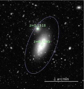
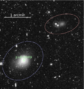
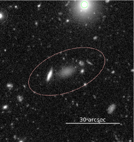
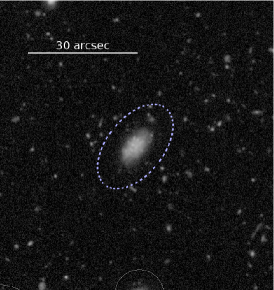
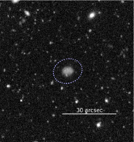
Figure 2.— Examples of dwarf galaxies from our sample in the $g$-band. The gray circles show the masked areas due to bright stars (Section 3.1). The ellipses around the galaxies at the center indicate the identified dwarf galaxies. The top row is for secure dwarfs (solid ellipses), while the bottom row is for possible dwarfs (dashed ellipses). The red and blue ellipses are for red and blue dwarfs (see Section 4.4), respectively. Galaxies with spec-$z$’s are indicated as such.

Although the surface brightness cut leaves only $\sim 0.2$ % of the objects in the original catalog, there is still a lot of contamination. The final stage of the dwarf galaxy selection is to remove the remaining contamination. For a small number of bright galaxies, secure spectroscopic redshifts from SDSS ($\rm zWarning=0$) are available. Spectroscopic objects in the background of the central galaxies are all removed at this point, although there are only a few such galaxies due to the surface brightness cut. A major source of the remaining contamination here is background (bulge-less) face-on spiral galaxies, which have low surface brightness.

We have experimented a few methods to distinguish dwarf galaxies from background face-on spirals, but it turned out that visual inspection is an efficient way to distinguish them because eye can easily tell whether a galaxy has spiral arms or not. A major downside is that a visual inspection is subjective and we ultimately require spectroscopic confirmations of all the dwarf galaxies. As we will discuss later, Prime Focus Spectrograph (PFS), which has a similar field of view to that of HSC, is the most efficient follow-up facility. For the purpose of the paper, we need conservative classifications and we introduce two classes of dwarfs: secure dwarf and possible dwarf. The former comprises galaxies that we judge highly likely to be real dwarf galaxies. This class includes confirmed dwarf galaxies with spectroscopic redshifts from SDSS ($\lesssim 100\ \rm km\ s^{-1}$ from the centrals). Also, galaxies with very smooth morphology are in this class. Possible dwarfs are less likely, but some of them may be real dwarfs and we keep them in the catalog. These possible dwarfs are typically small and have weak structure such as knots, which could possibly be a part of spiral arms or tidal features. Fig. 2 shows some of the secure and possible dwarf galaxies after this visual screening. All this is done in the $g$-band to fully utilize the superb seeing.

During this screening phase, we found that some of the dwarf galaxies are likely associated to a few extended background galaxies (their spatial distribution is clearly clustered around the background galaxies). We cannot distinguish dwarf galaxies around the targets from those around the background galaxies using surface brightness alone. As this is a major source of contamination, we choose to apply an additional mask around these background galaxies. We find that the virial radii of our target galaxies are about $100-200$ times the Kron radii, thus we use circular masks of radius $200r_{kron}$ around the background galaxies. We apply masks to all bright ($g<18$) galaxies that do not pass the surface brightness cut (i.e., dwarf galaxy candidates are not masked). This magnitude cut is conservative because we do not observe a clear clustering of dwarf galaxies around $g>17$ galaxies with the surface brightness cut we apply. This contamination of extended background galaxies is a lesson we learned from our pilot run. As described earlier, we have observed the virial regions of 5 central galaxies; 3 galaxies that we do not discuss in this paper happen to have a larger number of bright background galaxies, which makes it difficult to construct a clean sample of dwarf galaxies. In our on-going HSC observations, the number of bright background galaxies is included as an additional constraint.

In total, we identify 9 secure dwarfs and 4 possible dwarfs around N2950. N3245 has 13 secure and 2 possible dwarfs. These are raw counts from the observation and we apply the completeness correction described below when we discuss LFs in Section 4.1.

3.4. Detection Completeness

Having carefully screened the list of dwarf galaxy candidates, we now describe simulations to estimate the detection completeness of our method. We put artificial objects in the images with a wide range of sizes and luminosities, apply the same object detection, the same surface brightness cut, and the same masks. We repeat this procedure to estimate the fraction of objects with a given size and luminosity that can be detected with our procedure. For simplicity, we assume that all the dwarf galaxies have exponential radial profiles (effective radius and magnitudes are free parameters).

Fig. 3 shows our detection completeness as a function of size and luminosity. As can be seen, we detect most of the dwarf galaxies in the LG. The surface brightness cut is carefully chosen to include the majority of the LG dwarf galaxies, while keeping the contamination of background sources minimal. In other words, Fig. 3 motivated the surface brightness cut in Fig. 1. We do miss 3-4 % of the known LG dwarfs and they are very compact galaxies such as M32. However, M32 is unlike any other galaxy in the LG and we consider that such compact dwarfs are too rare to significantly affect our conclusion.

In addition to the completeness, we can also estimate biases in the total magnitude measurements from Source Extractor by comparing input photometry to the simulation and output photometry from Source Extractor. We find that the bias can be as large as $+0.15$ mag (output is fainter than input) for very diffuse sources. We correct for the photometry bias for all the detected dwarf candidates. In the same way, we correct for biases in the measurements of effective radius, which we will discuss later in the paper.

3.5. Statistical Field Subtraction

Finally, we consider contamination of field dwarf galaxies (i.e., isolated dwarf galaxies that are not satellites of any other galaxies). It is not clear how abundant such galaxies are, but we can eliminate them statistically using a control field sample, which does not contain any nearby large galaxies. For this control sample, we reduce public data in ELIAS-N1 from Hyper Suprime-Cam Subaru Strategic Program (HSC-SSP; Aihara et al. 2018a, 2018b) with the same configuration used in the processing of the target galaxies and stacked to similar depths. These data have identical seeing to ours, making it a good control sample. We apply the same object detection, masks, surface brightness cut, and visual inspections. We find that the surface density of field dwarfs is small ($\sim 1.4$ per square degree), and is not a major source of contamination. Nonetheless, we multiply the surface density with the effective surface areas of our target fields and the contamination of field dwarf galaxies is statistically subtracted when we discuss LFs.

4. Results

We now present the LFs of the dwarf galaxies we have detected around N2950 and N3245 and compare them with that of the MW and also with predictions from numerical simulations. We further discuss the size-luminosity relation, color-magnitude diagram, and the spatial distribution of the dwarf galaxies.

4.1. Luminosity Function

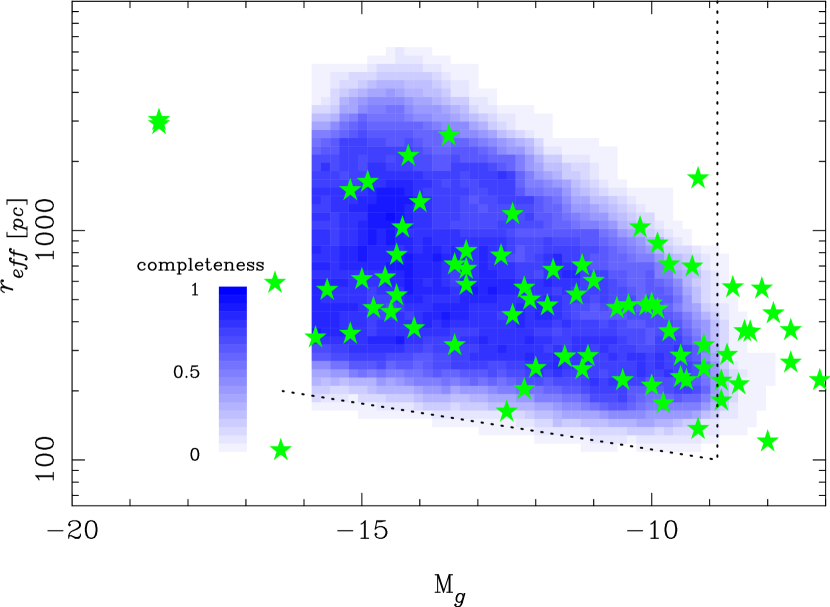
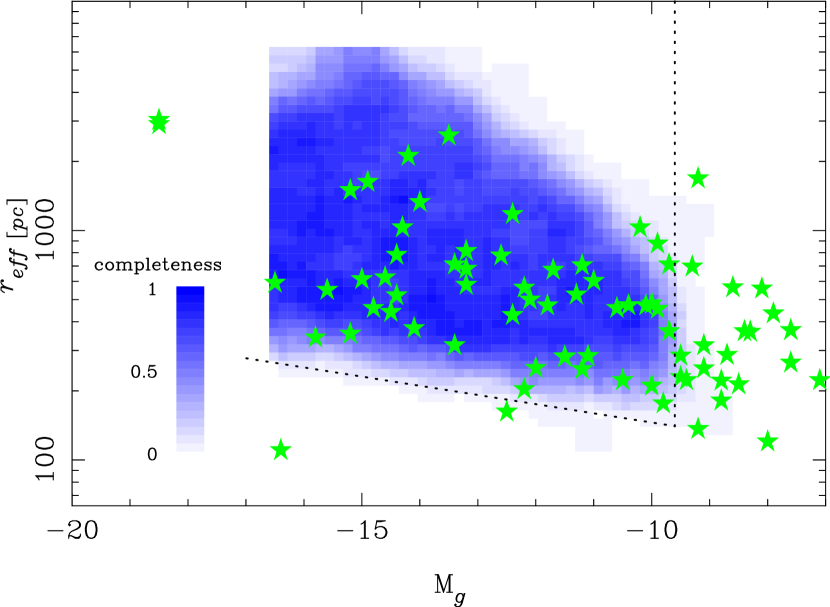
Figure 3.— Selection completeness as a function of absolute magnitude and effective radius. The left panel is for N2950 and the right for N3245. The bluescale shows the completeness and the stars are the dwarf galaxies in the LG. The dashed line shows the imposed magnitude and surface brightness cut in Fig. 1. The hard edges correspond to the parameter range we explore in the simulation ($100\rm\ pc$ $<r_{eff}<6000\rm\ pc$ and $15<g<23$). Note that the bright and very compact galaxy with $M\sim-16$ and $r_{eff}\sim 100$ pc is M32 and we are missing such very bright but compact dwarfs.

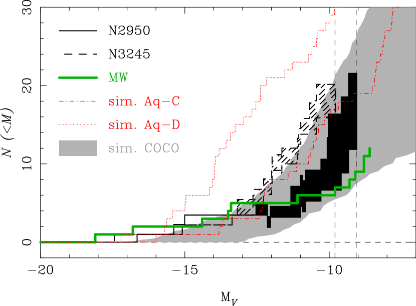
Figure 4.— Cumulative LFs of the observed dwarf galaxies (black solid and dashed lines) and MW (green solid). The black filled/hatched area in the observed LFs show the range of cumulative numbers of dwarf galaxies with secure dwarfs (lower boundary) and both secure and possible dwarfs (upper boundary). Note that the completeness correction has been applied to these LFs. The observed LFs go down at a few places due to the statistical field subtraction. The vertical lines indicate our magnitude cut ($g<22$). Tables 3 and 4 summarize the observed LFs of N2950 and N3245, respectively. The LFs from the simulations by Okamoto (2013) are shown as the red dotted and dot-dashed lines and the 68% range of the LFs from the COCO simulations is indicated as the gray shade. Note the large diversity of the LFs both in observation and simulation.

4.1.1 Comparison with the MW

We first compare the cumulative LFs of dwarf galaxies around our two target galaxies with that of the MW from McConnachie (2012). The MW LF is not complete at faint magnitudes, but for the brighter satellites we focus on here, the incompleteness correction is negligible (Tollerud et al., 2008; Newton et al., 2017). The virial radius ($r_{200}$) of the MW is not known very accurately, but we adopt 250 kpc (Bland-Hawthorn & Gerhard, 2016). We assume the MW halo mass of $1-2\times 10^{12}\rm M_{\odot}$ as described earlier and this virial radius is on the massive end of this halo mass range.

In order to compare with these literature results, we translate the $g$-band magnitudes into the $V$-band using

$$V=g-0.07-0.32\times(g-i),$$ (1)

which is derived from the Pickles (1998) stellar library. This may not be a very precise translation because it is based on stars, not galaxies. But, we do not need it to be very precise for the purpose of this pilot study.

Fig. 4 shows our primary result from the pilot observation. Although we have applied a fairly conservative magnitude cut to reduce contamination of artifacts and background sources, our LFs reach $V\sim-9.5$ mag. The shaded region of the observed dwarf LFs indicate the contribution of the possible dwarfs. We find that the MW LF is broadly consistent with N2950, although N2950 hosts a larger number of satellites at the faintest magnitudes probed. On the other hand, N3245 has more dwarfs than the MW by more than a factor of two. All these central galaxies have similar halo masses, but the satellite LFs seem to show a large diversity. This diversity is an important implication, but we first compare with numerical simulations before we discuss the diversity further.

4.1.2 Comparison with simulations

We compare the observed LFs with those from the numerical simulations of Okamoto (2013), who present high-resolution simulations of two MW-mass halos taken from the Aquarius project (Springel et al. 2008: ’Aq-C’ and ’Aq-D’ in their labeling system). Both halos have mass of $\rm M_{200}\sim 1.8\times 10^{12}M_{\odot}$. They are essentially higher resolution versions of the simulations of the Aq-C and Aq-D galaxies in Okamoto et al. (2010), in which they study satellites of MW-mass galaxies. While the simulation code used in Okamoto (2013) has been updated from Okamoto et al. (2010) for a better numerical convergence, the changes do not affect the satellite properties. The supernova feedback used in Okamoto (2013) is modeled as energy-driven winds, whose initial wind speed scales with the dark matter velocity dispersion. Okamoto et al. (2010) find that this feedback simultaneously explains the faint-end slope of the LF and the metallicity-luminosity relation of the Local Groups satellites.

In addition to Okamoto (2013) models, we also compare with predictions from the Galform semi-analytic model of Lacey et al. (2016) applied to the COCO $N$-body simulation (Hellwing et al., 2016) with tidal stripping of satellite galaxies accounted for using the STINGS particle tagging technique of Cooper et al. (2013, 2017). Details of the model is provided in the Appendix. COCO contains 90 isolated dark matter halos in the mass range $5\times 10^{11}<M_{200}/M_{\odot}<4\times 10^{12}$. For each of these, we construct satellite LFs using only the stars associated with $N$-body particles bound to surviving subhalos. The Lacey et al. (2016) model predicts the full SED of each stellar population, from which we compute the $V$-band luminosity of each satellite. We estimate the range enclosing 68% of the distribution of cumulative LF amplitude for these systems.

The model predictions are summarized in Fig. 4. All of these predictions are not convolved with any observational effects. For instance, our observations miss compact dwarf galaxies, while the simulations do not. Although we do not expect that compact dwarfs significantly affects our conclusion, we should forward-model the simulations to include these effects for more fair comparisons in our future work. With this caveat in mind, we find that one of the Okamoto (2013) model (Aq-C) is roughly consistent with N3245, whereas the other one (Aq-D) has more brighter dwarfs. COCO reproduces the observed range of LFs, although the two galaxies are still too limited to draw significant conclusions. One important implication of Fig. 4 is that both observations and models suggest a large diversity in the LFs. Indeed, there is about a factor of $\sim 2$ scatter at $M_{V}=-10$, although the main host galaxies all have similar halo masses.

There are a few possible reasons for the scatter. One is the scatter in our halo mass estimates. Stellar mass estimates from broadband photometry often have at least a factor of $\sim 2$ uncertainties due to a number of assumptions employed in the stellar population synthesis. There is additional scatter coming from the abundance matching relation between stellar mass and halo mass; both uncertainty on the mean relation and intrinsic scatter (Moster et al., 2010). Another contribution to the scatter may be physical variation in the LF at fixed mass. The accretion histories of halos of the same mass are not the same; some halos assemble a large fraction of their mass at early times, while others assemble late. The diversity in the accretion histories of galaxies may introduce further scatter (Boylan-Kolchin et al., 2010)

The observed diversity provides a compelling motivation for us to construct a statistically representative sample of nearby galaxies to fully test the missing satellite problem. We should not perform any cosmological tests using only a single halo (i.e., MW), assuming that it is representative of galaxies of similar stellar mass or halo mass. In fact, there are indications that the MW is not typical (e.g., Mutch et al. 2011; Tollerud et al. 2011; Rodríguez-Puebla et al. 2013). We are carrying out further observations to construct a larger sample and we discuss our future directions in Section 5.

4.2. Comparisons with literature

Geha et al. (2017) presented a spectroscopic campaign of nearby galaxies with MW-like mass with the same goal of addressing the missing satellite problem as this work. We have no galaxies in common with their sample, making direct comparisons difficult. However, it is still very useful to compare our LFs with theirs given the similarities in the target selection (we both target nearby galaxies with MW-like mass).

Fig. 5 makes this comparison. We apply an approximate transformation of the SDSS system into the $V$-band using the Pickles (1998) library in the same way as done in Eq. 1. Our LFs are in good agreement with those from Geha et al. (2017). This is reassuring because the methods to identify dwarf galaxies are quite different (photometry vs. spectroscopy). Geha et al. (2017) covered a relatively bright magnitude range and each galaxy has only a few to several satellites. On the other hand, we go $\sim 2.5$ magnitudes deeper and most of our dwarf galaxies are fainter than their limit. This nicely illustrates the complementarity and strength of our work.

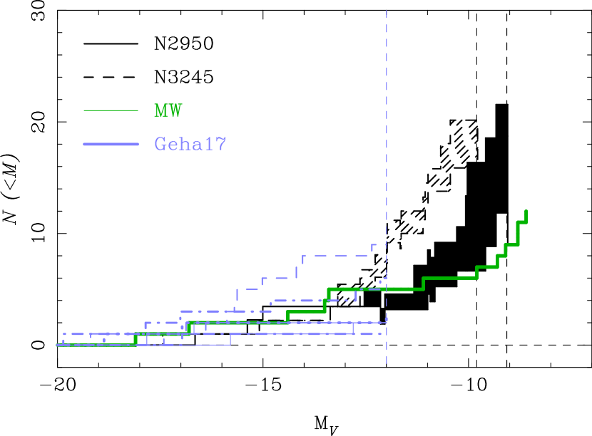
Figure 5.— Cumulative LFs of our sample (black solid and dashed lines) and MW (green solid) as in Fig. 4. The blue lines with various line styles are the satellite LFs from Geha et al. (2017). The dashed vertical lines indicate the limiting magnitudes of Geha et al. (2017), N3245, and N2950 from the left to the right.

Table 3Luminosity Function for N2950

$M_{V}$	$N_{upper}$	$N_{lower}$
$-16.65$	$1.00$	$1.00$
$-15.38$	$2.26$	$2.26$
$-15.01$	$3.47$	$3.47$
$-12.54$	$4.84$	$3.47$
$-12.14$	$3.27$	$1.90$
$-12.03$	$4.56$	$3.19$
$-11.33$	$7.14$	$3.19$
$-10.99$	$8.52$	$4.58$
$-10.93$	$7.84$	$3.90$
$-10.82$	$9.19$	$5.25$
$-10.29$	$10.60$	$6.66$
$-10.07$	$13.36$	$6.66$
$-10.03$	$16.36$	$6.66$
$-9.59$	$18.55$	$8.85$
$-9.33$	$21.55$	$11.85$

Table 4Luminosity Function for N3245

$M_{V}$	$N_{upper}$	$N_{lower}$
$-17.44$	$1.00$	$1.00$
$-15.09$	$2.21$	$2.21$
$-13.37$	$3.44$	$3.44$
$-13.18$	$5.44$	$3.44$
$-12.87$	$5.45$	$3.46$
$-12.64$	$6.75$	$4.75$
$-12.27$	$8.09$	$6.09$
$-11.99$	$9.34$	$7.34$
$-11.98$	$11.18$	$9.18$
$-11.66$	$10.64$	$8.64$
$-11.64$	$12.01$	$10.01$
$-11.11$	$13.25$	$11.25$
$-11.06$	$14.53$	$12.53$
$-10.99$	$15.79$	$13.79$
$-10.68$	$18.06$	$13.79$
$-10.44$	$20.15$	$15.88$

4.3. Size-Luminosity Relation

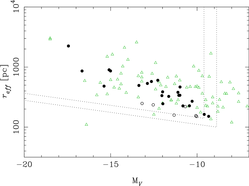
Figure 6.— Effective radius plotted against absolute magnitude. The black filled circles and open circles show the secure and possible dwarf galaxies around the target galaxies, respectively. The green triangles are the dwarf galaxies in the LG (McConnachie, 2012). The dotted lines indicate our magnitude and surface brightness cuts applied in the sample selection for N2950 (outer boundary) and N3245 (inner boundary), respectively. The data points are fewer than the number of dwarfs indicated in Fig. 4, but that is due to the completeness correction applied in Fig. 4.

Because the dwarf galaxies are fully resolved in the HSC images, we examine the relationship between $r_{eff}$ and luminosity. The MW dwarf galaxies are known to follow a clear size-luminosity relation and we here test whether the dwarf galaxies outside of the LG follow the same relation. We correct for any bias in our $r_{eff}$ from Source Extractor using the simulations described in Section 3.4 by making an empirical mapping between $r_{eff,obs}$ and $r_{eff,sim}$ as a function of magnitude and size, as done for completeness (Fig. 3).

Fig. 6 shows the size-luminosity relation of the dwarf galaxies. Our dwarf galaxies seem to follow the same relation as the MW dwarf galaxies, suggesting that the size-luminosity relation is universal. The possible dwarfs (open circles) tend to have smaller sizes than the secure dwarfs (filled circles), but that is obviously a bias that smaller objects are more difficult to classify.

Compared to the MW dwarfs, there are fewer faint but extended dwarf galaxies around our targets (e.g., $M_{V}\sim~{}-10$ and $r_{eff}\sim 500\rm\ pc$). We suspect it is due to combination of poor statistics and incompleteness. Our completeness is not very low for those objects (Fig. 3), but it is where the completeness starts to decrease. We apply the statistical correction to account for such incompleteness when we draw the LFs, but the statistical correction does not work if we detect no objects at all in a given (mag, $r_{eff}$) bin. This in turn suggests that our LFs shown in Fig. 4 may be incomplete at the faintest mags probed. Improved statistics from our future observations will allow us to draw more complete LFs.

4.4. Color-Magnitude Relation

To gain further insights into the nature of the dwarf galaxies, we plot a color-magnitude diagram in Fig. 7. We perform the $i$-band photometry using the dual image mode of Source Extractor to measure the $g-i$ color. We use MAG_AUTO here. We find that the dwarf galaxies have a range of $g-i$ color. This is not surprising given that some dwarfs are undergoing star formation with clumpy morphology, while others show only a smooth profile, which is typical of quiescent galaxies, as shown in Fig. 2. The possible dwarfs tend to be blue galaxies. Again, this is likely a selection bias in the sense that it is more difficult to distinguish dwarfs from background spiral galaxies if they have clumpy morphology. Smooth galaxies with no indication of on-going star formation are easier to classify.

In addition to the dwarf galaxies studied here, we plot brighter galaxies drawn from SDSS. These are spectroscopic galaxies from the Main sample (Strauss et al., 2002) at $z<0.07$ and are $k$-corrected to $z=0$ using Blanton & Roweis (2007). There is a clear bimodality of giant galaxies; red sequence and blue cloud. If we fit a line to the red sequence and extend it to fainter mags as shown by the solid line, we find that many of the red dwarf galaxies are nicely located around that line. This suggests that the red sequence extends at least to this faint magnitude. It also suggests that a large fraction of the observed dwarf galaxies are red galaxies and are not actively forming stars. The blue cloud is less clear at faint mags, but it may simply be due to the poor statistics. We split the dwarf galaxies into red and blue populations using the dotted line in the figure and examine their spatial distribution with respect to the central galaxy in the next subsection.

The Next Generation Virgo Cluster Survey (Ferrarese et al., 2012) also studied the faint end of the red sequence (Roediger et al., 2017). We show their functional fit to the red sequence in Virgo as the blue dashed curve in Fig. 7. The curve is translated into the HSC system using the Pickles (1998) library as done above. We find that the curve is in good agreement with the line fit to the SDSS data and also with the location of our dwarf galaxies. As we exclude groups and clusters from the target selection, our galaxies are a fair sample of field galaxies. The observed agreement suggests that the location of the red sequence is not strongly dependent of environment. This trend has been observed at bright magnitudes (e.g., Hogg et al. 2004; Tanaka et al. 2005), but this work extends it to much fainter magnitudes, $M_{V}\sim-9.5$.

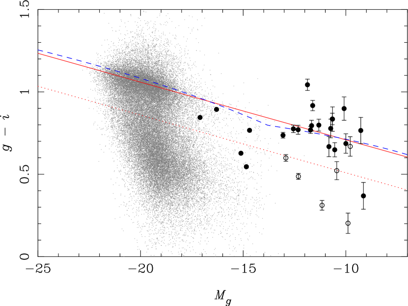
Figure 7.— $g-i$ plotted against $g$. The large points are the dwarf galaxies studied in this paper. As in the previous figures, the filled and open points are the secure and possible dwarfs, respectively. The gray dots are from SDSS. The solid line is a fit to the SDSS data only. The dashed line is the fit shifted by $\Delta(g-i)=-0.2$, which divides the dwarfs into red and blue galaxies. The blue dashed curve is the red sequence fit by Roediger et al. (2017).

4.5. Spatial Distribution

The dwarf galaxies in the LG have been known to distribute in two relatively thin 2D planes around the MW and M31 (Lynden-Bell, 1976; Ibata et al., 2013). This satellite alignment is potentially another challenge to $\Lambda$CDM (Ibata et al., 2013; Pawlowski & Kroupa, 2013; Pawlowski et al., 2015), although the statistical significance of these claims is disputed (Cautun et al., 2015; Shao et al., 2016). But, it is not easy to fully map out the distribution of dwarf galaxies in the LG because they literally spread all over the sky and some regions of the sky are difficult to observe (e.g., Galactic bulge). We can address this important question from a different perspective by studying the distribution of satellites around our targets in projection, as shown in Fig. 8.

We characterize the angular distribution of the dwarf galaxies with respect to the central galaxy. For this purpose, we use only the secure dwarfs in order to reduce possible contamination as we do not need a complete sample of dwarf galaxies here. To account for the complex masks we have applied, we draw random points within the $r_{200}$ of the central galaxies taking into account the masks, and compare the angular distribution of the dwarf galaxies with respect to that of the random points. The distribution within each angular bin is described as

$$P(\theta)=\frac{N_{D}(\theta)}{N_{R}(\theta)},$$ (2)

where $\theta$ is the projected angle of a dwarf galaxy measured with respect to the major axis of the host galaxy. $N_{D}(\theta)$ is the weighted number of satellite galaxies in bin $\theta$, while $N_{R}(\theta)$ is the number of random points in the same bin. The normalization of this distribution is defined by $\sum_{\theta}N_{D}(\theta)/N_{R}(\theta)$. Then, the cumulative distribution function (CDF) is given by

$$CDF=\sum_{\leq\theta}\frac{N_{D}(\theta)}{N_{R}(\theta)}.$$ (3)

Fig. 9 shows the CDFs of the angular separations (angular range from $0^{\circ}$ to $180^{\circ}$) of the dwarfs for each target. We restrict $\theta$ to the range $[0^{\circ},180^{\circ}]$, and thus projected positions of satellites with respect to their host are folded up into the first and second quadrants. The dwarf galaxies around N2950 seems to be preferentially located along the minor axis of the central galaxy (CDF goes above the random points around $\theta\sim 90^{\circ}$). As for N3245, the trend is less clear, but the CDF is below the random points along the minor axis and the dwarf galaxies seem to be more preferentially located along the major axis.

However, these trends do not seem to be statistically significant. We randomly draw the same number of random points as the observed number of secure dwarfs and perform the Kormogorov-Smirnov test between their CDFs. We repeat this procedure $10^{6}$ times and we cannot reject the null hypothesis ($p>0.05$ for $>97\%$ of the time). Thus, there is no strong evidence for satellite alignments around the targets. We consider that this is an interesting avenue to statistically address the satellite plane problem when a larger sample of galaxies with MW-like mass is available. Spectroscopic confirmations of the dwarf galaxies will also help. We will elaborate on our future direction in the next section.

In addition to the overall distribution of the dwarf galaxies, it is interesting to ask where the red and blue dwarfs are located with respect to the central galaxy. Interestingly, there is no significant correlation of the distribution of red/blue galaxies with respect to the central galaxy. The radial dependence of the red/blue fraction is consistent with flat (plot not shown) due to the large statistical error even when we combine the two targets. Again, this is a topic we will revisit with improved statistics in the future.

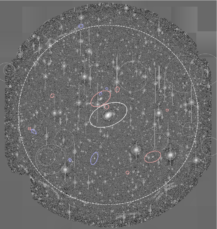
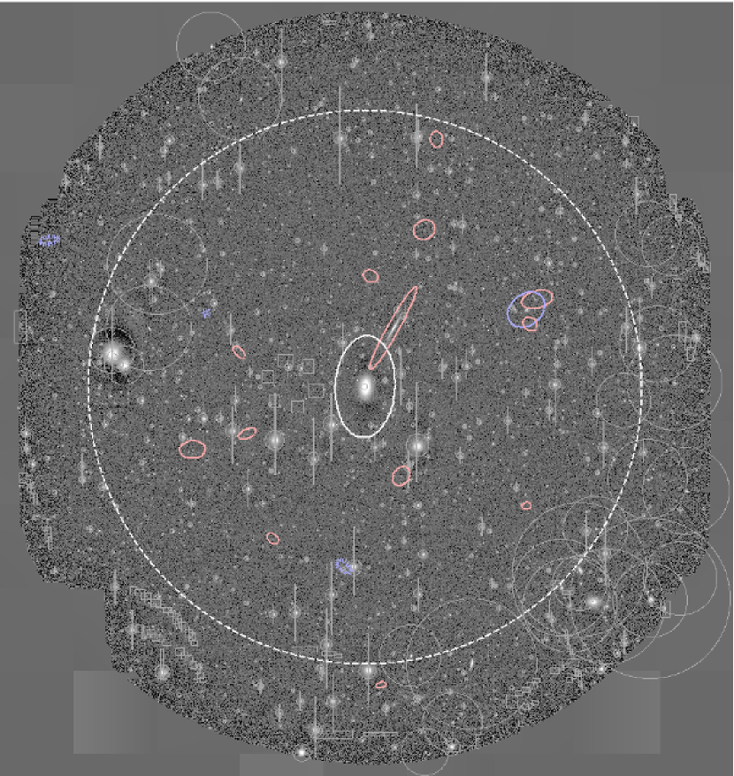
Figure 8.— Spatial distribution of the dwarf galaxies. The left and right panels are for N2950 and N3245, respectively. The gray boxes and circles show the masked regions due to bright stars, nearby background galaxies, and optical ghosts. The red/blue ellipses indicate the locations of the red/blue dwarf galaxies, respectively, and the solid and dashed ellipses are the secure and possible dwarfs. These ellipses are scaled Kron ellipses to indicate the shapes and sizes of the satellite galaxies. The outer dashed circles is the virial radius of the central galaxy.

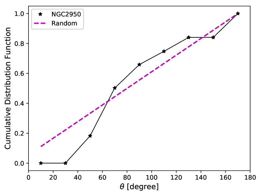
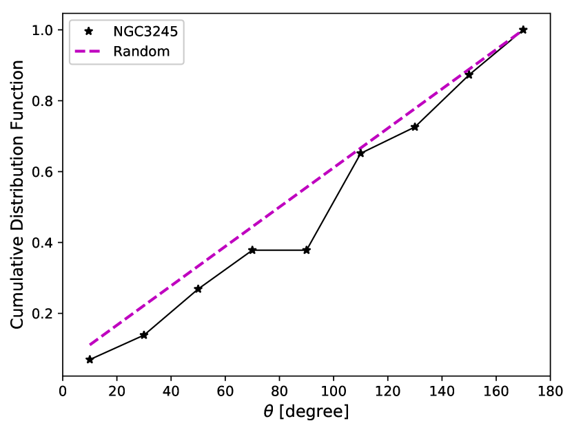
Figure 9.— The normalized cumulative distribution function (CDF) of angular separation of the satellites for NGC2950 (left) and NGC3245 (right). The magenta dashed lines show the CDFs using random points to represent a homogeneous distribution, while the black solid lines are the measured CDFs of the dwarf galaxies.

5. Summary and Discussion

We have presented the LFs of dwarf galaxies around two nearby (15–20 Mpc) galaxies with MW-like mass observed with HSC. At this distance, dwarf galaxies are spatially extended and we use this property to largely eliminate background sources and select a high purity sample of dwarf galaxy candidates by applying a surface brightness cut. Our data are of high quality and we achieve $\sim 0.5$ arcsec seeing in the $g$-band, which turns out to be critically important to distinguish dwarf galaxies from background face-on spirals (which also have low surface brightness). We statistically subtract any remaining contamination using a control field sample, which is processed in exactly the same manner as the targets. We also carefully account for the detection incompleteness and biases in our magnitude and size measurements using the simulations.

Our primary results are (1) the satellite LF of N2950 is broadly consistent with that of the MW, whereas N3245 has a more abundant dwarf population, (2) the observed LFs are on average about a factor of two smaller than prediction from the hydrodynamical simulations of Okamoto (2013), while COCO reproduces the observed LFs well and importantly (3) there is a large diversity in the LFs both in the observations and simulations. The last point highlights the importance of addressing the missing satellite problem with a statistically representative sample. We have also examined the size-luminosity relation and found that the dwarfs around our targets follow the same relation as the MW dwarfs. The $g-i$ color of the dwarf galaxies spans a wide range, but many of them have red colors consistent with the red sequence of massive galaxies extrapolated to faint magnitudes. Finally, we have looked at the spatial distribution of the dwarf galaxies, but we do not observe strong evidence for the alignment of satellites around the central galaxies.

Given these promising results, our next step is to increase the sample size to fully constrain the satellite abundance of MW analogues and so address a number of related challenges to $\Lambda$CDM. We are carrying out further HSC observations of nearby galaxies and we plan to report on their LFs in a subsequent paper. Our final sample will comprise both early- and late-type galaxies and it will be interesting to examine the dependence of dwarf galaxy properties on the central galaxy properties. Also, it will be important to extend the mass range; there is no reason why we should stick with MW-like mass and a sample with a wider mass range will give us a wider leverage to test the models. In addition, we will explore a more sophisticated algorithm to identify faint dwarfs. We have examined the LFs down to $\sim-9.5$ mag in this paper, but as mentioned earlier, that is not a limit imposed by the data. A more sophisticated method should allow us to probe fainter dwarf galaxies.

Finally, we remind ourselves that our selection of dwarf galaxies is based on the surface brightness selection. We need spectroscopic confirmations of the dwarf galaxies to derive more reliable LFs. It is not practical to follow-up all possible candidates with any of the existing spectroscopic facilities, but Prime Focus Spectrograph (PFS; Tamura et al. 2016) is an ideal instrument. PFS is a massively multiplexed fiber spectrograph ($\sim 2400$ fibers) to be mounted on the Subaru telescope and its field of view is nearly as large as that of HSC, which makes it possible to follow-up all the possible candidates in one go. We plan to perform an intensive follow-up programme with PFS in order to confirm dwarf satellite candidates and derive more secure LFs in our future work.

Appendix A Copernicus Complexio (COCO) Simulation

COCO is a cosmological zoom simulation of an approximately spherical high-resolution region of radius $\sim 25\rm\ Mpc$ (resembling the Local Volume) embedded within a periodic box of $100\rm\ Mpc$/side simulated at lower resolution. Particles in the high-resolution region have mass $m_{p}=1.612\times 10^{5}\rm\ M_{\odot}$ (hence the low-mass dwarf galaxy hosts are resolved with $\sim 5000$ particles) and softening length $\epsilon=0.327\rm\ kpc$. COCO assumes the WMAP-7 cosmological parameters.

Galform (Cole et al., 2000) models galaxy formation as a network of coupled differential equations describing processes including the evolving thermal state of cosmic gas and the interstellar medium, star formation and energetic feedback from supernovae and supermassive black holes. Free parameters in the model are written in terms of physical (observable) quantities and calibrated against a wide range of statistical data from surveys of the galaxy population on cosmologically representative scales. We use Galform (as described in Lacey et al. 2016) to predict the star formation history of every self-bound dark matter halo in COCO, and hence the stellar masses of surviving satellite galaxies around MW-like hosts at $z=0$. Bose et al. (2017) present a detailed analysis of MW-like satellite populations in the Lacey et al. (2016) model applied to COCO. Guo et al. (2015) also discuss the satellites of Milky Way analogues in COCO, using an alternative semi-analytic model.

The default Lacey et al. (2016) model does not include gradual stellar mass loss from satellites due to tidal stripping. We account for this using the particle-tagging technique STINGS described by Cooper et al. (2010, 2013). STINGS uniformly distributes the stellar mass of every unique single age stellar population (comprising all stars formed in a specific halo between two successive simulation output times, according to Galform) over a set of dark matter particles. Each set of ’tagged’ particles is chosen to approximate the phase-space distribution of its associated stellar population at the time of its formation (for details see Cooper et al. 2017) and can be used to trace its subsequent evolution in phase space.

References

- Aihara et al. (2018a) Aihara, H., Armstrong, R., Bickerton, S., et al. 2018, PASJ, 70, S8
- Aihara et al. (2018b) Aihara, H., Arimoto, N., Armstrong, R., et al. 2018, PASJ, 70, S4
- Axelrod et al. (2010) Axelrod, T., Kantor, J., Lupton, R. H., & Pierfederici, F. 2010, Proc. SPIE, 7740, 774015
- Bertin & Arnouts (1996) Bertin, E., & Arnouts, S. 1996, A&AS, 117, 393
- Bland-Hawthorn & Gerhard (2016) Bland-Hawthorn, J., & Gerhard, O. 2016, ARA&A, 54, 529
- Blanton & Roweis (2007) Blanton, M. R., & Roweis, S. 2007, AJ, 133, 734
- Bose et al. (2017) Bose, S., Hellwing, W. A., Frenk, C. S., et al. 2017, MNRAS, 464, 4520
- Boylan-Kolchin et al. (2010) Boylan-Kolchin, M., Springel, V., White, S. D. M., & Jenkins, A. 2010, MNRAS, 406, 896
- Boylan-Kolchin et al. (2011) Boylan-Kolchin, M., Bullock, J. S., & Kaplinghat, M. 2011, MNRAS, 415, L40
- Bruzual & Charlot (2003) Bruzual, G., & Charlot, S. 2003, MNRAS, 344, 1000
- Cautun et al. (2015) Cautun, M., Bose, S., Frenk, C. S., et al. 2015, MNRAS, 452, 3838
- Chabrier (2003) Chabrier, G. 2003, PASP, 115, 763
- Cole et al. (2000) Cole, S., Lacey, C. G., Baugh, C. M., & Frenk, C. S. 2000, MNRAS, 319, 168
- Cooper et al. (2010) Cooper, A. P., Cole, S., Frenk, C. S., et al. 2010, MNRAS, 406, 744
- Cooper et al. (2013) Cooper, A. P., D’Souza, R., Kauffmann, G., et al. 2013, MNRAS, 434, 3348
- Cooper et al. (2017) Cooper, A. P., Cole, S., Frenk, C. S., Le Bret, T., & Pontzen, A. 2017, MNRAS, 469, 1691
- Ferrarese et al. (2012) Ferrarese, L., Côté, P., Cuillandre, J.-C., et al. 2012, ApJS, 200, 4
- Geha et al. (2017) Geha, M., Wechsler, R. H., Mao, Y.-Y., et al. 2017, ApJ, 847, 4
- Gilmore et al. (2007) Gilmore, G., Wilkinson, M. I., Wyse, R. F. G., et al. 2007, ApJ, 663, 948
- Guo et al. (2015) Guo, Q., Cooper, A. P., Frenk, C., Helly, J., & Hellwing, W. A. 2015, MNRAS, 454, 550
- Hellwing et al. (2016) Hellwing, W. A., Frenk, C. S., Cautun, M., et al. 2016, MNRAS, 457, 3492
- Hogg et al. (2004) Hogg, D. W., Blanton, M. R., Brinchmann, J., et al. 2004, ApJ, 601, L29
- Ibata et al. (2013) Ibata, R. A., Lewis, G. F., Conn, A. R., et al. 2013, Nature, 493, 62
- Ivezic et al. (2008) Ivezic, Z., Axelrod, T., Brandt, W. N., et al. 2008, Serbian Astronomical Journal, 176, 1
- Jarrett et al. (2000) Jarrett, T. H., Chester, T., Cutri, R., et al. 2000, AJ, 119, 2498
- Jarrett et al. (2003) Jarrett, T. H., Chester, T., Cutri, R., Schneider, S. E., & Huchra, J. P. 2003, AJ, 125, 525
- Jurić et al. (2015) Jurić, M., Kantor, J., Lim, K., et al. 2015, arXiv:1512.07914
- Kauffmann et al. (1993) Kauffmann, G., White, S. D. M., & Guiderdoni, B. 1993, MNRAS, 264, 201
- Klypin et al. (1999) Klypin, A., Kravtsov, A. V., Valenzuela, O., & Prada, F. 1999, ApJ, 522, 82
- Kuzio de Naray et al. (2008) Kuzio de Naray, R., McGaugh, S. S., & de Blok, W. J. G. 2008, ApJ, 676, 920-943
- Lacey et al. (2016) Lacey, C. G., Baugh, C. M., Frenk, C. S., et al. 2016, MNRAS, 462, 3854
- Licquia & Newman (2015) Licquia, T. C., & Newman, J. A. 2015, ApJ, 806, 96
- Lynden-Bell (1976) Lynden-Bell, D. 1976, MNRAS, 174, 695
- Magnier et al. (2013) Magnier, E. A., Schlafly, E., Finkbeiner, D., et al. 2013, ApJS, 205, 20
- Makarov et al. (2014) Makarov D., Prugniel P., Terekhova N., Courtois H., & Vauglin I. 2014, A&A, 570, A13
- McConnachie (2012) McConnachie, A. W. 2012, AJ, 144, 4
- McGaugh et al. (2001) McGaugh, S. S., Rubin, V. C., & de Blok, W. J. G. 2001, AJ, 122, 2381
- Miyazaki et al. (2012) Miyazaki, S., Komiyama, Y., Nakaya, H., et al. 2012, Proc. SPIE, 8446, 84460Z
- Moore et al. (1999) Moore, B., Ghigna, S., Governato, F., et al. 1999, ApJ, 524, L19
- Moster et al. (2010) Moster, B. P., Somerville, R. S., Maulbetsch, C., et al. 2010, ApJ, 710, 903
- Mutch et al. (2011) Mutch, S. J., Croton, D. J., & Poole, G. B. 2011, ApJ, 736, 84
- Newton et al. (2017) Newton, O., Cautun, M., Jenkins, A., Frenk, C. S., & Helly, J. 2017, arXiv:1708.04247
- Okamoto et al. (2010) Okamoto, T., Frenk, C. S., Jenkins, A., & Theuns, T. 2010, MNRAS, 406, 208
- Okamoto (2013) Okamoto, T. 2013, MNRAS, 428, 718
- Parry et al. (2012) Parry, O. H., Eke, V. R., Frenk, C. S., & Okamoto, T. 2012, MNRAS, 419, 3304
- Pawlowski & Kroupa (2013) Pawlowski, M. S., & Kroupa, P. 2013, MNRAS, 435, 2116
- Pawlowski et al. (2015) Pawlowski, M. S., Famaey, B., Merritt, D., & Kroupa, P. 2015, ApJ, 815, 19
- Pickles (1998) Pickles, A. J. 1998, PASP, 110, 863
- Rodríguez-Puebla et al. (2013) Rodríguez-Puebla, A., Avila-Reese, V., & Drory, N. 2013, ApJ, 773, 172
- Roediger et al. (2017) Roediger, J. C., Ferrarese, L., Côté, P., et al. 2017, ApJ, 836, 120
- Sawala et al. (2016) Sawala, T., Frenk, C. S., Fattahi, A., et al. 2016, MNRAS, 457, 1931
- Sawala et al. (2016) Sawala, T., Frenk, C. S., Fattahi, A., et al. 2016, MNRAS, 456, 85
- Schlafly et al. (2012) Schlafly, E. F., Finkbeiner, D. P., Jurić, M., et al. 2012, ApJ, 756, 158
- Schlegel et al. (1998) Schlegel, D. J., Finkbeiner, D. P., & Davis, M. 1998, ApJ, 500, 525
- Shao et al. (2016) Shao, S., Cautun, M., Frenk, C. S., et al. 2016, MNRAS, 460, 3772
- Sheth et al. (2010) Sheth, K., Regan, M., Hinz, J. L., et al. 2010, PASP, 122, 1397
- Skrutskie et al. (2006) Skrutskie, M. F., Cutri, R. M., Stiening, R., et al. 2006, AJ, 131, 1163
- Springel et al. (2008) Springel, V., Wang, J., Vogelsberger, M., et al. 2008, MNRAS, 391, 1685
- Strauss et al. (2002) Strauss, M. A., Weinberg, D. H., Lupton, R. H., et al. 2002, AJ, 124, 1810
- Tamura et al. (2016) Tamura, N., Takato, N., Shimono, A., et al. 2016, Proc. SPIE, 9908, 99081M
- Tanaka et al. (2005) Tanaka, M., Kodama, T., Arimoto, N., et al. 2005, MNRAS, 362, 268
- Tollerud et al. (2008) Tollerud, E. J., Bullock, J. S., Strigari, L. E., & Willman, B. 2008, ApJ, 688, 277-289
- Tollerud et al. (2011) Tollerud, E. J., Boylan-Kolchin, M., Barton, E. J., Bullock, J. S., & Trinh, C. Q. 2011, ApJ, 738, 102
- Tonry et al. (2001) Tonry, J. L., Dressler, A., Blakeslee, J. P., et al. 2001, ApJ, 546, 681
- Tonry et al. (2012) Tonry, J. L., Stubbs, C. W., Lykke, K. R., et al. 2012, ApJ, 750, 99
- Wang & White (2012) Wang, W., & White, S. D. M. 2012, MNRAS, 424, 2574
- York et al. (2000) York, D. G., Adelman, J., Anderson, J. E., Jr., et al. 2000, AJ, 120, 1579