A technique for plasma velocity-space cross-correlation

Abstract

An advance in experimental plasma diagnostics is presented and used to make the first measurement of a plasma velocity - space cross - correlation matrix. The velocity space correlation function can detect collective fluctuations of plasmas through a localized measurement. An empirical decomposition, singular value decomposition, is applied to this Hermitian matrix in order to obtain the plasma fluctuation eigenmode structure on the ion distribution function. A basic theory is introduced and compared to the modes obtained by the experiment. A full characterization of these modes is left for future work, but an outline of this endeavor is provided. Finally, the requirements for this experimental technique in other plasma regimes are discussed.

I Introduction

Kinetic modes, defined here as solutions to a plasma kinetic equation, have recently been used to describe phenomena in astrophysical plasmasKlein et al. (2012), low density plasmasSkiff et al. (2002); De Souza-Machado, Sarfaty, and Skiff (1999); Diallo and Skiff (2005), and fusion plasmasHatch et al. (2011); Terry, Baver, and Gupta (2006); Terry et al. (2014). Kinetic modes’ importance is partially due to the need to overcome the shortcomings of fluid and magnetohydrodynamic descriptions that capture only a few modes in the full plasma collective mode spectrum. This collective mode spectrum requires a different mathematical approach that can give a general description of dynamics in collisionlessVan Kampen (1955); Case (1959) and weakly collisional plasmasNg, Bhattacharjee, and Skiff (2004). A problem remains that these kinetic modes, usually being small and localized, are difficult to isolate experimentally. We seek to introduce a new method that may be useful for detecting and measuring these modes.

Often, kinetic modes can be best detected through phase space resolving diagnostics. In our case, we use a phase space correlation measurement. Correlations of plasma quantities have an extensive history, with recent examples using densityTolias et al. (2015), magnetic fieldsBhat and Subramanian (2015), and field - particle correlationsKlein and Howes (2016); Howes, Klein, and Li (2017) to investigate fluctuations, magnetic power spectra, and collisionless energy transfer in turbulence respectively. This illustrates a useful property of correlation functions: depending on the plasma quantities correlated, they provide insight into specific aspects of plasma behavior.

The main velocity sensitive diagnostic used in this paper is laser induced fluorescence (LIF). It fits the criteria of being phase space resolving and, with our setup, is able to measure a phase space correlation of plasma ion distribution fluctuations:

$$C(\vec{x}_{1},\vec{x}_{2},\vec{v}_{1},\vec{v}_{2},\tau)=\langle\delta f(\vec{x}_{1},\vec{v}_{1},t)\delta f(\vec{x}_{2},\vec{v}_{2},t-\tau)\rangle_{t}$$ (1)

where $\langle\rangle_{t}$ denotes a time average and $\delta f=f-\langle f\rangle_{t}$ is the phase space distribution function fluctuation. This particular correlation can provide insight into plasma kinetic modes.

This work stands on a foundation of previous LIF measurements of $C$. They employed a single laser, measuring $C$ for $v_{1}=v_{2}$, to measure LIF at two separate points along the laser beamFasoli, Skiff, and Tran (1994) and to measure $C$ as a function of $v_{1}=v_{2}$ and with varying separation $x_{1}-x_{2}$Diallo and Skiff (2005). Bicoherence spectra were also derived from these measurementsUzun-Kaymak and Skiff (2006). We build on these measurements by introducing a localized measurement technique that measures $C$ for $x_{1}=x_{2}$ as a function of two separate and adjustable velocities $v_{1}$ and $v_{2}$. By varying these velocities, a matrix of cross correlations in velocity space may be obtained.

In this Paper, we introduce a technique combining the velocity sensitive diagnostic LIF with a velocity space correlation. Thus we demonstrate with this technique the first measurement of a plasma velocity – space cross – correlation matrix. It is possible that the measurement, due to measurement complications, is valid at some frequencies but not at others. We show how to verify the measurement through symmetry properties of the matrix. By applying a singular value decomposition to this Hermitian correlation matrix, we obtain the velocity space degrees of freedom of the plasma fluctuations as a function of frequency. We also compare the eigenmodes given by the singular value decomposition to a basic kinetic theory.

Our goal here is to introduce a new measurement technique, independent of velocity resolving diagnostic, that provides a new velocity space perspective of plasma fluctuations. This technique can detect kinetic modes in plasma through a localized measurement. We want to emphasize that while we demonstrate this measurement with laser induced fluorescence (LIF), it is applicable where any velocity sensitive measurement is available and a multipoint measurement may be difficult. Examples of this include a satellite with numerous velocity sensitive instruments, several collective Thomson schemes focused on one point in a fusion plasma, trapped plasmasAnderegg et al. (1997), or laser cooled plasmasStrickler et al. (2016). To further the goal of introducing a useful measurement technique, we briefly discuss the criteria and pitfalls in applying this measurement to other plasmas at the conclusion of this paper.

The velocity sensitive diagnostic in this experiment, laser induced fluorescence (LIF), is traditionally used to measure moments of the plasma distribution function such as density, temperature, average velocity, and higher. Moments are the easier measurements with this diagnostic. The fact that LIF is a velocity sensitive diagnostic means that fundamental plasma properties can be measured with it. There is a history of intricate measurements of fundamental plasma properties using laser induced fluorescence, including early optical tagging measurementsStern (1985), wave – particle interactionFasoli et al. (1993), phase space response to linear and nonlinear waves and phase bunchingMcWilliams and Sheehan (1986), and plasma presheath measurementsOksuz, Khedr, and Hershkowitz (2001); Hood et al. (2016). All of these LIF measurements surmount the issue of photon statistics noise. In our experiment there is a twofold contribution to noise. First, there is a large contribution ($>90\%$ of signal) from collision induced background fluorescence. Second, LIF itself is limited to low photon rates by low metastable state densities and thus we have issues with photon counting statistics.

Correlations offer a way to remove this noise, in addition to providing a measure of a useful plasma quantity. By using ensemble averaging, we can isolate and eliminate the photon statistics noise. However, this is still a technically difficult measurement to perform with LIF, which is why only the above mentioned handful of correlation measurements with LIF exist. For this reason, we quantify both the efficiency of background noise subtraction of the collisionally induced fluorescence and whether we have counted enough photons through symmetry properties of the velocity – space cross correlation matrix. With this, we show how the measurement can be verified.

II Experimental Setup

The experiment is performed on a cylindrical axially magnetized singly ionized Argon (Ar II) plasma generated from an RF inductively coupled antenna of length $2.3$ m and radius $\approx 2.5$ cmDiallo and Skiff (2005). The magnetic field is .67 T. Langmuir probe measurements show ion and electron densities of $n\approx 9*10^{9}$ cm^-3 and $T_{e}\approx 9$ eV. LIF reveals $T_{i}\approx 0.08$ eV though the distribution has significant deviations from a Maxwellian. Ion neutral collisions have frequency $\nu\approx 500$ Hz. The plasma has ambient acoustic and drift wave fluctuations above the thermal noise level, but they are small due to convective stabilization. An antenna driven with white noise drives fluctuations in the plasma. The plasma chamber contains two separate and independently movable carriages with light collection optics for measuring LIF. We leverage their independence to make this measurement.

The measurement setup is shown in Fig. 1. Two separate lasers are combined using a dichroic mirror, filtered for a single linear polarization with a Glan laser prism, right hand circularly polarized with a quarter waveplate, and then sent into the plasma. The exclusive right hand circular polarization eliminates the left hand Zeeman splitting subgroup. Similarly, laser propagation parallel to the magnetic field removes the $\pi$ perpendicular Zeeman patternCondon and Shortley (1959).

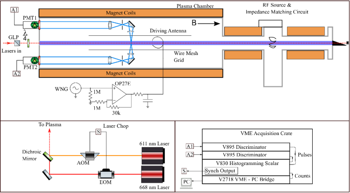
Figure 1: Experimental setup. Top: The full plasma chamber setup. Two independently movable carriages within the plasma chamber have collecting optics for gathering, collimating, and sending out LIF light to PMTs 1 and 2. GLP is a Glan Laser Prism and $\lambda/4$ is a quarter wave plate. A single loop antenna is upstream of the viewing volume and is driven with an amplified white noise signal from the white noise generator (WNG). Bottom Left: Laser set up. The two lasers are combined with a dichroic mirror with 650 nm cutoff (Thorlabs DMSP650). Each laser is amplitude modulated according to a data acquisition synchronized signal fed into an acousto-optical modulator (AOM) for the 611 nm laser and an electro-optical modulator for the 668 nm laser. Bottom right: The PMT pulse digitization and readout scheme. The signals from the PMTs enter discriminators (V895), which digitize the PMT pulses. These pulses are histogrammed with a V830, which also outputs a logic signal for laser modulation according to the histogramming logic. Finally, the results are read out to a PC via the V2718 and written to disk.

Each laser excites a separate independent laser induced fluorescence scheme. Laser 1, a TOptica TA 100 Diode laser, excites the ArII metastable state ⁴F_7/2 with 668nm to ⁴D${}^{\circ}_{5/2}$ which decays to ⁴P_3/2, emitting light at 442 nm; laser 2, a Matisse Rhodamine 6G Dye laser, excites ²G_9/2 with 611nm to ²F_7/2 which decays to ²D_5/2, emitting light at 461nm. Each laser absorption spectrum is broadened by the same ion velocity distribution function, and each laser is velocity sensitive since the laser bandwidth is $<1$ MHz.

These two laser induced fluorescence schemes must be isolated - otherwise transitions between the excited states can affect the cross correlation. There are two major sources of transitions: collision induced transitions and atomic transitions. Collision induced transitions may be immediately disregarded, since their frequency at 500 Hz is very low compared to the atomic transition frequency of 100 MHz. If an atomic transition pathway exists, however, the cross correlation can be affected. We searched for a pathway experimentally by modulating two separate lasers and looking for a beat frequency $f=f_{1}\pm f_{2}$. No beat frequency was found and so we believe that a pathway does not exist for our particular laser induced fluorescence schemes we have chosen. Any new pair of LIF schemes to repeat this measurement will need to be verified similarly.

Both sets of collection optics in the chamber are focused at the same point with volume $0.20$ cm³. Since the lasers are spatially combined but independently tunable over velocity, and the optics are focused at the same point, we are obtaining a measurement of the cross correlation function $C(v,v^{\prime},\tau)$ at two points separated in velocity space.

III Measuring the Velocity – Space Cross – Correlation

We can now measure the velocity – space cross – correlation matrix. The measured matrix is a three dimensional matrix of velocity $\cdot$ velocity $\cdot$ time. The first two dimensions, in velocity, are selected by each laser, while the third dimension (time) corresponds to the $\tau$ of the cross correlation $C(v_{1},v_{2},\tau)$.

We begin by measuring the full ion velocity distribution function with each laser. We select points on the distribution corresponding to the peak, 2/3 of the peak, 1/2 of the peak, 1/3 of the peak, and one point on the tail for seven points total. Figure 2 shows the measured IVDF and the measurement points on it. At each possible combination of the lasers, we measure the time series data $f(v_{1},t)$ from laser 1 and $f(v_{2},t)$ from laser 2. After demodulation with respect to 100 kHz laser chopping, the mean is subtracted to provide the fluctuation $\delta f=f-<f>_{t}$. Cross correlating and averaging with respect to $t$ gives the cross correlation $C(v_{1},v_{2},\tau)$ for each of the selected velocities. This gives an 8 x 8 x (2 N - 1) matrix where the first two dimensions are the velocities selected by each laser and the last dimension is the time separation $\tau$.

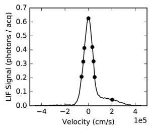
Figure 2: Deconvolved ion velocity distribution function measured by the two independent LIF schemes. The solid line is the ion velocity distribution function measured with a traditional lock in amplifier setup and laser wavelength sweep. The anomalous Zeeman effect has been removed via deconvolution. The circles are the measurement points at the peak, 2/3 of the peak, 1/2, 1/3, and on the tail of the distribution. This shows a typical IVDF in the plasma; the prominent tail at high positive velocities is also visible.

Accomplishing this measurement with LIF is technically difficult and requires a large amount of time to overcome photon counting statistics noise, even after the background noise from collision induced fluorescence is subtracted. The data presented here took three weeks of continuous steady state plasma operation and data acquisition. In addition to the reduction of noise through this ensemble averaging, we suppress photon noise and background fluorescence at several points: stray light filtering in the set up; background light subtraction through LIF signal demodulation (this step removes background light correlation as well); filtering via a Gaussian windowing function of the time correlation; and the suppression of photon noise statistics through time ensemble averaging. The last point is possible since the plasma is steady state. Validating that this noise reduction works is important, so we examine properties of the cross correlation matrix.

Ideally, the cross correlation matrix $C(v_{1},v_{2},\tau)$ is symmetric such that it equals $C(v_{2},v_{1},-\tau)$. However, the measured data are not perfectly symmetric. There are errors in wavelength selection, and the magnetic field induces slightly different Zeeman broadening in each laser’s absorption spectrum. This breaks the velocity space symmetry. Due to the low magnetic field of 0.67 T and single circular polarization, the Zeeman subgroup spacing is small compared to the measurement spacing. This is shown by the near symmetry of the actual raw data matrix.

With the $C(v_{1},v_{2},\tau)$ matrix in hand, we can quantify the degree of broken symmetry, and thus, whether the noise suppression worked. The following procedure gives where the measurement does have good symmetry as a function of frequency. First, split the cross correlation matrix into symmetric and antisymmetric components $S,A=\textonehalf C(v,v^{\prime},\tau)\pm C(v^{\prime},v,-\tau)$. Then take the Fourier transform of $S$ and $A$ in order to obtain $\tilde{S}$ and $\tilde{A}$, which are exactly Hermitian and antihermitian in the 2D velocity space by construction. By a close form of the Fourier convolution theorem, $\tilde{S}$ and $\tilde{A}$ are equal to the complex conjugate multiplied symmetric and antisymmetric components of $\delta f(v,t)$ and $\delta f(v^{\prime},t)$, and the absolute value is the cross power spectrum. By comparing the cross power spectra of $\tilde{S}$ and $\tilde{A}$, we can verify the measurement is symmetric, and thus, our noise reduction techniques are successful and external systematic effects are not too strong.

We choose a physically motivated example, drift waves, for verification of this process. Consider the physical set up in Fig.3. The periscopes are oriented at $90^{\circ}$ to each other and each has two light collection volumes overlapping at the focus - where the lasers are located. Pinholes ensure rejection of stray light outside the focus, but crucially it is not complete rejection. While the lasers are at this localized point, the optics collect light from the entire volume. The drift wave amplitude peaks in the gradient region of the plasma - higher up in the collection region and away from the focus. With this physical set up in mind, we quantify how the matrix symmetry can be broken - and indeed identify at what frequencies the cross power spectrum of the two lasers dominates, as opposed to other phenomena not in the laser region. According to the measured plasma parameters and adjusting for the $k_{\perp}$ imposed by the wire mesh grid, we expect a drift frequency $f^{*}\approx 10$ kHz. Additionally, we expect a phase near $f^{*}$ of $\pi/2$, since the strongest drift wave mode corresponds to the first Fourier mode decomposition $e^{im\varphi}$ where $m=1$Horton (1999) and the periscope optics are oriented at $90^{\circ}$. In all, we expect the antihermitian and Hermitian power spectra to approach each in other in strength and the phase of the antihermitian spectrum to be $\pi/2$ near $f^{*}$. Figure 4 confirms this. The antihermitian component approaches the Hermitian component near $f^{*}$, and the inset shows the phase at $\pi/2$ verifies our expectations given the physical set up of the system.

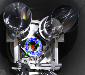
Figure 3: Photograph of the interior of the plasma chamber. This is from the perspective of the lasers that enter the chamber. The overlay describes important geometry of the experiment: red is the laser volume; green is the light collection volume; and blue is an idealized drift signature. The light collection volume is so shaped due to a pinhole. This shows, physically, why we expect the $\pi/2$ phase contribution to the data matrix at $f^{*}$. Incidentally it also shows the two separate carriages inside the plasma chamber. Collimated light going towards the PMT is going out of the page.

As a result, frequencies where the magnitude of the Hermitian component dominate over the antihermitian component are where the measurement is successful. This shows that not only have we suppressed background noise and photon statistics, but that the Zeeman subgroup spacing is not too large. For our particular measurement, this is true - to 10dB or better - for frequencies below $f^{*}$. Thus we have a measurement of the velocity - space cross - correlation function and have quantified for which frequencies it is valid. We have measured $C(v,v^{\prime},\tau)$ at these frequencies. For these frequencies, obtaining the velocity space degrees of freedom and their eigenmodes on the plasma ion velocity distribution function is now possible.

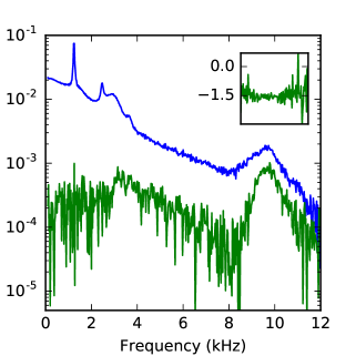
Figure 4: Representative power spectrum of a single velocity pair’s time cross correlation. The larger blue spectrum is the Hermitian component while the smaller green spectrum is the antihermitian component. The inset shows the phase of the antihermitian component at the drift frequency and has the same abscissa as the outer figure. Reproduced from S. Mattingly and F. Skiff, Phys. Plasmas 24 (2017), 10.1063/1.4996012 with permission from AIP Publishing.

IV Velocity Space Degrees of Freedom

We apply an empirical data transform, singular value decomposition (SVD)Nardone (1992), in order to determine the velocity space degrees of freedom of the plasma. We apply it to the Hermitian matrix $\tilde{S}(v,v^{\prime},\tau)$. Since this matrix is exactly Hermitian by construction, it is diagonalizable. Thus the singular vectors returned by SVD are the eigenvectors and the singular values are the absolute values of the eigenvalues. These singular values are the relative strengths of their corresponding singular vectors. Physically, the singular values can be interpreted as the strengths of the different wave modes comprising the plasma fluctuations at a single point in frequency. Write $\delta f$ as a sum of wave modes and expand $C(v,v^{\prime})$:

$$\delta f(v)=\sum_{i}^{n}a_{i}f_{i}(v)$$ (2)

$$C(v,v^{\prime}) =\langle\delta f(v)\delta f(v^{\prime})\rangle_{t}=\sum_{i}^{n}a_{i}f_{i}(v)\sum_{j}^{n}a_{j}f_{j}(v^{\prime})$$

$$=\sum_{i}^{n}|a_{i}|^{2}f_{i}(v)f_{i}(v^{\prime})+\sum_{i\neq j}^{n}a_{i}a_{j}f_{i}(v)f_{j}(v^{\prime})$$ (3)

Here, $f_{i}$ is a wavemode. In the case of linearly independent plane modes, the cross terms cancel out and we are left only with the simple basis $\sum_{i}^{n}|a_{i}|^{2}f_{i}(v)f_{i}(v^{\prime})$.

If the plasma modes are constituted of fluctuations that are linear and independent as shown above, then singular value decomposition of the measured $C(v,v^{\prime},f)$ matrix would be very useful - it would diagonalize the matrix and pluck out the modes $f_{i}(v)$ and their strengths $|a_{i}|^{2}$. These strengths $|a_{i}|^{2}$ correspond to the real valued singular values returned by SVD. They are the velocity space degrees of freedom.

However, the shape of fluctuations, especially in velocity space, is not necessarily linear. In this case the above discussion is invalid since the cross terms of Eqn. 3 would no longer cancel out. SVD’s ansatz that the basis is linear and orthogonal causes it to fail in this case. Determining and applying a suitable transform for this case is a major avenue for future work which we discuss in more detail in the final parts of this paper. For now, we apply SVD to $C(v,v^{\prime})$ keeping these drawbacks in mind.

We apply SVD to the two dimensional velocity space matrix at every point in the frequency spectrum. Assuming continuity of the eigenvectors across frequency, we connect the singular values across the spectrum. This process gives spectra showing the relative strengths of the detected plasma fluctuation modes as a function of frequency and are shown in Fig 5. These are the velocity space degrees of freedom. We consider these spectra in greater detail to demonstrate spatial mode separation from this localized measurement. Fully understanding these spectra is a point of active and future work.

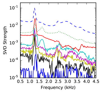
Figure 5: Power spectra from connecting the singular values of the Hermitian matrix. A separate SVD is run on each 2D velocity space and connecting the singular values across frequency gives this plot. The fact that these power spectra differ is evidence of distinct modes. The third strongest mode, in solid red, becomes second strongest around $1250\text{Hz}$ and then drops back to being third strongest. These are the velocity space degrees of freedom of plasma fluctuations as a function of frequency. Reproduced from S. Mattingly and F. Skiff, Phys. Plasmas 24 (2017), 10.1063/1.4996012 with permission from AIP Publishing.

The large peak at 1250 Hz matches the frequency of an ion acoustic bounded mode in the plasma chamber with frequency given by $c_{s}/\lambda$, where $c_{s}$ is the ion acoustic speed and $\lambda$ the wavelength of the bounded mode. Here, this wavelength is $\lambda=460$ cm, twice the length of the plasma column. This peak has harmonics at 2500 Hz and 3750 Hz. The appearance of this mode in all the SVD spectra shows a failure of the method at this particular wavelength - the ion acoustic bounded mode is strong enough that it may be nonlinearly scattering into the other modes. This causes the nonlinear terms of Eqn. 3 to be nonzero.

The peak at 1600 Hz and its harmonic at 3200 Hz are, we believe, due to a longitudinal bounded mode in the wire mesh grid. The same calculation above for the 1250 Hz peak, only with the dimensions of the wire mesh grid, gives these frequencies. But this is due to a rough estimate; we do not actually know what the boundary conditions are at the end of the mesh grid. There are no observations on a bounded mode like this to the authors’ knowledge. Still, this mode shows both advantages and limitations of the SVD method. First of all, the peak at 1600 Hz is not apparent in the original power spectrum of Fig. 4. However, SVD clearly separates it into the second and fourth spectra. This is an example of separating modes with this localized measurement. This may also be a failure case - it may be a nonlinear mode that SVD fails to separate. Alternatively, it is possible that there are two modes present which SVD is separating into these separate strengths. Finally, the peak at 3200 Hz may not be a harmonic as the Lorentzian broadening (Q factor) is not explained by calculations assuming reasonable reflection coefficients from the open ended mesh grid. An intriguing possibility has been suggested that it may be due to nonlinear interactions between the two 1600 Hz modes or the 1600 Hz and 1250 Hz modes. Sorting all this out is a point of present and future work.

The second strongest SV mode, colored with a green dotted line in Fig. 5, becomes third strongest near 1250 Hz. We find this by examining the singular value’s corresponding eigenvectors as the frequency is varied; specifically, we minimize the difference in eigenvectors for adjacent points on the frequency axis. By enforcing this, we find that the second and third SV modes switch in strength before and after the peak near 1250 Hz. This exemplifies SVD’s lack of knowledge outside the frequency it is applied. Because it is a 2D transform applied repeatedly to 2D slices of a 3D matrix, it only has information on the particular 2D space it is run on. Still, we have pioneered a method of finding not only the relative strengths of these modes from a localized measurement, but also how they change in relative strength as a function of frequency. A point of future work is determining a transform that can incorporate the third dimension of the matrix for determining the mode strength as a function of frequency more reliably. This will be especially useful when the mode crossing behavior is not sharply defined, like it is in our case, but more gradual.

V Plasma Fluctuation Eigenmodes

Since the data matrix is Hermitian, singular value decomposition also gives complex valued eigenvectors $f_{i}(v)$ corresponding to the singular values. In the general non Hermitian case, these are the principal axes. We examine the shape of these eigenvectors, and introduce a basic theory in an attempt to explain some of them. The theory we introduce only meets with partial success; fully explaining the modes is an area that we believe is rich in future work.

For comparison, we introduce a basic kinetic theory based on electrostatic ion waves in a quasineutral plasma with Boltzmann electrons. We can obtain a useful form for $f_{1}$, the perturbed distribution function, which can match up with some (but not all) of the modes gives by the SVD analysis. First we write the Vlasov equation in Poisson bracket form with a Bhatnagar - Gross - Krook (BGK) operatorBhatnagar, Gross, and Krook (1954),

$$\partial f/\partial t+[f,H]=\nu(-f_{1}+f_{0}n_{1}/n_{0}),$$ (4)

and linearize, dropping second order terms. $\nu$ is the collision frequency. We use the ansatz $f_{1}=Ae^{-i\omega t+ik_{||}z+ik_{\perp}(X+\frac{v_{\perp}}{\Omega}sin\varphi)}$ with the gyrophase coordinate $X$ and expand $f_{1}$ in Bessel functions of the first kind to get

$$f_{1}=\sum_{n=-\infty}^{\infty}f_{n}J_{n}(k_{\perp}v_{\perp}/\Omega).$$ (5)

where $\Omega$ is the ion cyclotron frequency and $v_{\perp}$ is the perpendicular thermal velocity. By solving the linearized Vlasov equation for $f_{n}$, returning to $x$ from the gyrophase coordinate $x$, substituting the $f_{n}$ obtained from Eqn. 4 in the above $f_{1}$ expansion, and integrating over $v_{\perp}$, we obtain

$$f_{1}(v_{||})=\sum_{n=-\infty}^{\infty}e^{-k_{\perp}^{2}v_{T}^{2}/\Omega^{2}}I_{n}(\frac{k_{\perp}^{2}v_{T}^{2}}{\Omega^{2}})\frac{n_{1}}{n_{0}}k_{B}T_{e}$$

$$\times\frac{ik_{||}\frac{\partial f_{0}}{\partial p_{||}}+(\frac{in\Omega}{k_{B}T_{\perp}}+\frac{\nu}{k_{B}T_{e}})f_{0}}{\nu+ik_{||}v_{||}-i\omega-in\Omega},$$ (6)

where $I_{n}$ is a modified Bessel function of the first kind. According to this equation, at a given a frequency there are a range of modes present in the plasma where each mode $f_{1}$ has its own pair $k_{||}$ and $k_{\perp}$. It is not a dispersion relation. Similarly, SVD resolves a subset of modes for each given frequency and so we have separated the different spatial plasma modes with a single localized measurement in velocity space.

We attempt to categorize the measured modes using Eqn. 6. By evaluating Eqn. 6 using the measured plasma parameters, the collision frequency $\nu=500$ Hz, and a large range of $k_{\perp}$ and $k_{||}$; finding the norm of the difference between the obtained $f_{1}$ and the data derived eigenvector; and finding the minimum of the resulting surface of values, we obtain theory predicted values for the eigenvectors. It is interesting to note that one may also fit for the collision frequency, though we choose to keep it fixed at a realistic value. This could open another method of collision frequency estimation given a well understood mode in the future. The result of this process is shown for the two strongest eigenvectors in Fig. 6 for $f=800$ Hz. The data derived eigenvector for the next two weaker modes are also shown, though we are not able to fit them.

The strongest mode fits with the model for the tail and the sides of the distribution, but not at the peak of the distribution. It resembles a typical linearized ion acoustic wave response, only derived from the SVD analysis. The fitted parameters in Eqn. 6 are $\lambda_{||}\approx 14.6$ cm and $\lambda_{\perp}\approx 1.4$ cm. The second strongest mode does not fit as well due to divergence from the tail of the distribution; the shown mode’s fitted parameters are $\lambda_{||}\approx 460$cm and $\lambda_{\perp}\approx 15.3$cm.

This process does not work for all the vectors returned by SVD. The weaker modes are not explained at all by Eqn. 6. Understanding and fitting these modes is a point of future work. Still, we have demonstrated spatial mode separation from a localized velocity space measurement.

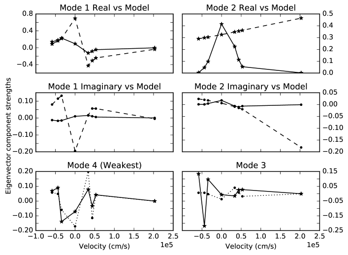
Figure 6: Eigenvectors of the four strongest singular value modes (in groups with strongest at top left; clockwise) at $f=800$ Hz. In the first two modes, solid lines are derived from the experimental data while dashed lines are derived from the model of Eqn. 6. The third and fourth modes are derived solely from the experimental data; no fit is available. For them, the solid lines are the real component while the dotted lines are the imaginary component. These results show that the strongest mode has the best fit, while the fit diverges for the tail point on the second strongest mode. This shows where our theory works, and where it breaks down.

VI Summary

In this paper, we have presented a new measurement technique for measuring a plasma fluctuation velocity-space cross-correlation matrix. We demonstrated the technique on a laboratory plasma device and thus obtained the first measurement of this matrix. By examining symmetry properties of the matrix, we verified the measurement for a range of frequencies. We further verify it with comparison to a prominent drift wave feature in our plasma. For these verified frequencies, we applied a singular value decomposition to the Hermitian velocity space correlation matrix. We discussed several longitudinal bounded modes in the plasma chamber and the wire mesh grid inside the plasma chamber, showing both advantages and drawbacks of SVD. These drawbacks readily lead to future work. In addition, we showed and discussed the eigenmodes on the plasma fluctuation distribution function given by SVD as well. Finally, we introduced a basic theory from a Vlasov equation with a BGK operator in order to make estimates of expected eigenmode shapes. This theory has apparent shortcomings, and only works for some eigenmodes, but not for others.

VII Future Work: Velocity Space Matrix Decomposition

A full characterization of the modes given by this experiment is a major avenue of future work. Finding and applying a theory based decomposition is intertwined in this. With a suitable theory based transform the problems inherent to SVD shown in the discussion of Eqn. 3 may be solved. With this in hand, one could more accurately characterize the plasma modes detected with the method presented here.

There are two major candidates, at the time of writing and to the authors’ best knowledge, for theory based transforms. The first is the Morrison $\mathscr{G}$ transformMorrison and Shadwick (1994), which transforms the collisionless linearized Vlasov - Poisson system onto a Case - van Kampen (CVK) mode basis. Applying a transform such as this to the measurement presented in this paper requires a great amount of experimental and theoretical work. First, the $C(v,v^{\prime})$ matrix would need to be created for a much larger number than 8 measurement points on the velocity distribution function. This is a technically difficult endeavor for LIF mainly due to counting statistics. Second, applying the $\mathscr{G}$ transform, a continuous transform, to the discrete data of this experiment needs to be accomplished. A $\mathscr{G}$ based analogue to the Nyquist sampling theorem and a generalized convolution theorem may be helpful for applying the $\mathscr{G}$ transform to a discretely sampled set of data.

Work on applying the $\mathscr{G}$ transform may also motivate the placement of the measurement points on the ion velocity distribution function. Traditional sampling theory dictates evenly spaced samples in order to perfectly reconstruct an underlying sinusoidal signal. This may not be the case for determining velocity space plasma modes from different measurement points on an ion distribution function. In the case of velocity space fluctuations the underlying fluctuations have a different form, and so a measurement “bunching” on areas on the velocity distribution function may be necessary. Study of the $\mathscr{G}$ transform may help determine where the measurement points of $C(v,v^{\prime})$ should be placed so that the $\mathscr{G}$ transform can properly extract the underlying modes.

Being able to reliably isolate CVK modes with this experimental technique and the $\mathscr{G}$ transform would open experimental investigation of damping mechanisms of CVK modes, which are not damped by Landau dampingStix (1992). Another possibility, which requires a generalized convolution theorem, is experimentally determining phase space fluctuation spectra of density, electric field, and other plasma quantities using this measurement technique and the $\mathscr{G}$ transformMorrison and Shadwick (2008).

The second major candidate for theory based transforms is through constructing Hermite polynomials for a weakly collisional plasmaNg, Bhattacharjee, and Skiff (2004); De Souza-Machado, Sarfaty, and Skiff (1999). This method uses Hermite polynomial expansions in the Vlasov equation with a Lenard - BernsteinLenard and Bernstein (1958) collision operator to find a discrete and infinite set of modes in velocity space. The Hermite polynomial expansion is intrinsically discrete, which may make applications to our dataset easier. Still, similar to the $\mathscr{G}$ transform, work on the Hermite expansion would be beneficial to identify the best measurement points and apply it to the Hermitian data derived matrix presented in this paper.

The Hermite expansion technique may also provide a sort of bridge between the current SVD methodology and a theory - driven transform. One may create a well known mode, such as the ion acoustic longitudinal bounded mode, and generate the Hermite polynomial adjoint matrix corresponding to the measurement points on the distribution function. By left multiplying this adjoint matrix with the Hermitian matrix at each frequency, then taking the singular value decomposition, we can determine whether the modes isolated by SVD correspond to the known modes. This is a point of future work.

Both of these transforms, $\mathscr{G}$ and Hermite, seek to sort out the underlying eigenmodes of the system. In an infinite and homogeneous system, the velocity-space cross-correlation eigenfunctions would be the plasma eigenmodes. However, there is scattering between these infinite plasma modes due to long correlation lengths, complicating the picture (and invalidating an analysis like the SVD used earlier for them). Projection onto either CVK modes or kinetic modes via the $\mathscr{G}$ transform and Hermite polynomial decompositions respectively could help to sort the situation out.

VIII Future Work: Application to other plasmas

For this method to be applied to other plasmas, there are a few requirements that the plasma system must fulfill. First, it must have two sets of independently tunable, velocity sensitive diagnostics focused on the same volume in the plasma. Ideally, they will be nonperturbative. We use LIF in this experiment, but other ways are possible. For example, a satellite with multiple Faraday cups tuned to separate velocities fits these criteria. Second, there must be a way of taking an ensemble average to overcome counting statistics. We accomplish this with a steady state plasma. But this is not the only way - a good counterexample is a recent heterodyne method with LIF on a pulsed Hall thrusterDiallo et al. (2015). Finally, the incoherent correlation length of the time cross correlation of $f(v,t)$ and $f(v^{\prime},t)$ must be short relative to a single time series dataset but long relative to the sampling rate.

IX Acknowledgements

This work is supported by the US DOE under the NSF-DOE program with grant number DE-FG02-99ER54543.

References

- Klein et al. (2012) K. G. Klein, G. G. Howes, J. M. Tenbarge, S. D. Bale, C. H. K. Chen, and C. S. Salem, Astrophys. J. 755 (2012), 10.1088/0004-637X/755/2/159.
- Skiff et al. (2002) F. Skiff, H. Gunell, A. Bhattacharjee, C. S. Ng, and W. A. Noonan, Phys. Plasmas 9, 1931 (2002).
- De Souza-Machado, Sarfaty, and Skiff (1999) S. De Souza-Machado, M. Sarfaty, and F. Skiff, Phys. Plasmas 6, 2323 (1999).
- Diallo and Skiff (2005) A. Diallo and F. Skiff, Phys. Plasmas 12, 110701 (2005).
- Hatch et al. (2011) D. R. Hatch, P. W. Terry, F. Jenko, F. Merz, and W. M. Nevins, Phys. Rev. Lett. 106, 115003 (2011).
- Terry, Baver, and Gupta (2006) P. W. Terry, D. A. Baver, and S. Gupta, Phys. Plasmas 13, 022307 (2006).
- Terry et al. (2014) P. W. Terry, K. D. Makwana, M. J. Pueschel, D. R. Hatch, F. Jenko, and F. Merz, Phys. Plasmas 21 (2014), 10.1063/1.4903207.
- Van Kampen (1955) N. G. Van Kampen, Physica 21, 949 (1955).
- Case (1959) K. Case, Ann. Phys. (N. Y). 7, 349 (1959).
- Ng, Bhattacharjee, and Skiff (2004) C. S. Ng, A. Bhattacharjee, and F. Skiff, Phys. Rev. Lett. 92, 065002 (2004).
- Tolias et al. (2015) P. Tolias, S. Ratynskaia, A. Panarese, S. Longo, and U. D. Angelis, J. Plasma Phys. 81, 1 (2015).
- Bhat and Subramanian (2015) P. Bhat and K. Subramanian, J. Plasma Phys. 81, 395810502 (2015).
- Klein and Howes (2016) K. G. Klein and G. G. Howes, Astrophys. J. Lett. 826, L30 (2016), arXiv:1607.01738 .
- Howes, Klein, and Li (2017) G. G. Howes, K. G. Klein, and T. C. Li, J. Plasma Phys. 83, 705830102 (2017), arXiv:1705.06385 .
- Fasoli, Skiff, and Tran (1994) A. Fasoli, F. Skiff, and M. Q. Tran, Phys. Plasmas 1, 1452 (1994).
- Uzun-Kaymak and Skiff (2006) I. Ü. Uzun-Kaymak and F. Skiff, Phys. Plasmas 13, 112108 (2006).
- Anderegg et al. (1997) F. Anderegg, X.-P. Huang, E. Sarid, and C. F. Driscoll, Rev. Sci. Instrum. 68, 2367 (1997).
- Strickler et al. (2016) T. S. Strickler, T. K. Langin, P. McQuillen, J. Daligault, and T. C. Killian, Phys. Rev. X 021021, 1 (2016), arXiv:1512.02288 .
- Stern (1985) R. A. Stern, Rev. Sci. Instrum. 56, 1006 (1985).
- Fasoli et al. (1993) A. Fasoli, F. Skiff, R. Kleiber, M. Q. Tran, and P. J. Paris, Phys. Rev. Lett. 70, 303 (1993).
- McWilliams and Sheehan (1986) R. McWilliams and D. Sheehan, Phys. Rev. Lett. 56, 2485 (1986).
- Oksuz, Khedr, and Hershkowitz (2001) L. Oksuz, M. A. Khedr, and N. Hershkowitz, Phys. Plasmas 8, 1729 (2001).
- Hood et al. (2016) R. Hood, B. Scheiner, S. D. Baalrud, M. M. Hopkins, E. V. Barnat, B. T. Yee, R. L. Merlino, and F. Skiff, Phys. Plasmas 23 (2016), 10.1063/1.4967870.
- Condon and Shortley (1959) E. U. Condon and G. H. Shortley, The Theory of Atomic Spectra (Cambridge University Press, 1959).
- Horton (1999) W. Horton, Rev. Mod. Phys. 71, 735 (1999).
- Nardone (1992) C. Nardone, Plasma Phys. Control. Fusion 34, 1447 (1992).
- Bhatnagar, Gross, and Krook (1954) P. L. Bhatnagar, E. P. Gross, and M. Krook, Phys. Rev. 94, 511 (1954).
- Morrison and Shadwick (1994) P. J. Morrison and B. A. Shadwick, Acta Phys. Pol. A Gen. Phys. 85, 759 (1994).
- Stix (1992) T. H. Stix, Waves in Plasmas, 2nd ed. (Springer-Verlag, New York, NY USA, 1992) pp. 308–309.
- Morrison and Shadwick (2008) P. J. Morrison and B. A. Shadwick, Commun. Nonlinear Sci. Numer. Simul. 13, 130 (2008).
- Lenard and Bernstein (1958) A. Lenard and I. B. Bernstein, Phys. Rev. 112, 1456 (1958).
- Diallo et al. (2015) A. Diallo, S. Keller, Y. Shi, Y. Raitses, and S. Mazouffre, Rev. Sci. Instrum. 86, 033506 (2015).