Velocity space degrees of freedom of plasma fluctuations

Abstract

We present the first measurements of a plasma velocity-space cross-correlation matrix. A singular value decomposition is applied to this inherently Hermitian matrix and the relation between the eigenmodes and the plasma kinetic fluctuation modes is explored. A generalized wave admittance is introduced for these eigenmodes.

Collective fluctuation modes of plasmas offer a general description of plasma dynamics in collisionless Van Kampen (1955); Case (1959) and weakly collisional plasmasNg, Bhattacharjee, and Skiff (2004). Kinetic modes have been studied both in low density plasmas Skiff et al. (2002); De Souza-Machado, Sarfaty, and Skiff (1999); Diallo and Skiff (2005) and in fusion plasmas, where in the latter they play an important role in the energetics of electrostatic turbulence and transportHatch et al. (2011); Terry, Baver, and Gupta (2006); Terry et al. (2014). Fluid and magnetohydrodynamic descriptions capture only a few modes in the full plasma collective mode spectrum. Understanding plasma fluctuations and transport requires the inclusion of kinetic modes. However, kinetic modes are difficult to isolate experimentally.

Detecting kinetic modes is best achieved by phase space resolving diagnostics. Here we employ laser induced fluorescence (LIF)Stern and Johnson (1975) to measure the plasma distribution fluctuation correlation function

$$C(\vec{x}_{1},\vec{x}_{2},\vec{v}_{1},\vec{v}_{2};\tau)=\langle\delta f(\vec{x}_{1},\vec{v}_{1},t)\delta f(\vec{x}_{2},\vec{v}_{2},t-\tau)\rangle_{t},$$ (1)

where $\langle\rangle_{t}$ denotes a time average and $\delta f=(f-\langle f\rangle_{t})$ is the phase space distribution function fluctuation.

Earlier LIF measurements of $C$ found the autocorrelation given by the diagonal $v_{1}=v_{2}$. Those measurements employed a single laser to measure fluorescence at two separate points along the laser beamFasoli, Skiff, and Tran (1994) and to measure $C$ as a function of single $v_{1}=v_{2}$ with separation $x_{1}-x_{2}$Diallo and Skiff (2005). Bicoherence spectra were also derived from these measurementsUzun-Kaymak and Skiff (2006). In this Letter, we employ a local measurement technique with $x_{1}=x_{2}$ and select two separate and adjustable velocities $v_{1}$, $v_{2}$ so that a matrix of cross correlations can be obtained.

By doing this, we present in this Letter the first measurements of a plasma velocity-space cross-correlation matrix. From this local measurement multiple degrees of freedom can be isolated, including the kinetic modes. We validate our noise reduction techniques through the symmetry properties of the fluctuation correlation function. We demonstrate this technique on a weakly coupled plasma and compute the associated eigenvectors in velocity space. A frequency dependent generalized wave admittance can be derived for each eigenmode.

The locality of the measurement means that the technique may be applied to plasmas in which a single-point velocity-sensitive measurement is possible and multipoint measurements may be difficult. Examples include in situ measurements of space plasmas, fusion plasmas, trapped plasmas Anderegg et al. (1997), and laser cooled plasmas Strickler et al. (2016).

While LIF is frequently used to measure slowly varying moments of the ion velocity distribution ($n$, $\vec{u}$, $T$, and higher), measuring fluctuations as required in this experiment is difficult due to photon statistics fluctuations that make a twofold contribution to noise. Firstly, the LIF photon count rate is limited due to low metastable state densities and the need to avoid excessive optical pumping. Secondly, a large fraction of the light signal is not from single frequency LIF itself but rather from electron collision-induced fluorescence. Collision-induced fluorescence affects ions at all velocities and is related to the metastable state populating mechanisms. Thus, collision-induced fluorescence is linked to the signal magnitude. Therefore, a statistical subtraction is needed.

Correlation measurements use ensemble averaging which permits evaluation and elimination of photon statistics noise. Nevertheless, there is only the above mentioned handful of phase space incoherent fluctuation measurements. For this reason, the efficiency of subtraction of the background fluorescence is a secondary question that we address in this Letter by exploiting symmetry properties of this correlation function.

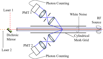
Figure 1: Experimental data acquisition scheme and setup. Two lasers, one at $668\text{nm}$ and one at $611\text{nm}$, are combined using a dichroic mirror and sent into the plasma. Corresponding to the two LIF schemes, PMT1 has a filter for 442nm while PMT2 has a filter for 461nm. An electrical white noise generator connected to a ring antenna excites the plasma modes with a broadband spectrum from $0-50$ kHz. A cylindrical mesh grid gives additional definition to radial mode structure.

The experiment is performed on an Argon II $13.56$ MHz RF inductively coupled magnetized ($B\approx 0.067$ T) cylindrical plasma column of length $2.3$ m and radius $r\approx 2.5$ cmDiallo and Skiff (2005). A Langmuir probe measures the ion and electron densities $n\approx 9\times 10^{9}~{}\text{cm}^{-3}$ and $T_{e}\approx 10~{}\text{eV}$. LIF reveals $T_{i}\approx 0.08~{}\text{eV}$, though there are significant deviations from a Maxwellian distribution. Ion neutral collisions have frequency $\nu\approx 500$ Hz. The ambient ion acoustic wave and drift wave amplitudes are above the thermal fluctuation level but are small due to convective stabilization. Additionally, a ring antenna driven with white noise excites broadband plasma modes in the system.

The experimental setup is shown in Fig 1. Two separate lasers are combined using a dichroic mirror and sent into the plasma to induce fluorescence on two different metastable lines. These lines must be isolated - otherwise transitions between the excited states can affect the laser optical correlation. We have tested for this direct atomic collisional-radiative connection through extensive searches for laser modulation frequency mixing, which was not detected. The underlying form of these isolated LIF excitation schemes are the same: laser 1 excites the ArII metastable state ${}^{4}\text{F}_{7/2}$ with 668 nm to ${}^{4}\text{D}^{\circ}_{5/2}$ which decays to ${}^{4}\text{P}_{3/2}$, emitting light at 442 nm; laser 2 excites ${}^{2}\text{G}_{9/2}$ with 611 nm to ${}^{2}\text{F}^{\circ}_{7/2}$ which decays to ${}^{2}\text{D}_{5/2}$, emitting light at 461 nm. The dominant broadening mechanism of the laser absorption spectrum is Doppler broadening and each laser absorption spectrum is broadened by the same plasma ion distribution function to within the noise level of 0.1%. Velocity selection is available with each tunable laser since the laser bandwidth is $<1~{}\text{MHz}$. Finally, to suppress the Zeeman pattern corresponding to the left circular polarization, these lasers are exclusively right circularized by passing them through a Glan-Taylor laser polarizer and a quarter wave plate. The low field of $0.067$ T limits the width of each $\sigma^{+}$ polarized Zeeman group.

In this experiment, the collection optics are focused at the same point with volume $0.20~{}\text{cm}^{3}$. Therefore, since the measurement scheme spatially combines the lasers and then obtains the correlation function at this physical volume, we obtain the correlation function of ions at two points separated in velocity phase space $C(v_{1},v_{2},\tau)$.

With this setup, first a full absorption spectrum is observed with each laser. We then choose a set of velocities across the distribution function: the peak of the distribution; $2/3$ the peak of the distribution; $1/2$ the peak; $1/3$ the peak; and one point on the tail. The ion velocity distribution function’s tail is due to how the plasma is produced Sarfaty, De Souza-Machado, and Skiff (1998)^,Skiff et al. (2000). In total, the same 8 velocity points are measured for each laser.

We then measure time series data $f(v,t)$ and $f(v^{\prime},t)$ for the full array of selected velocities. After demodulation with respect to $100$ kHz laser chopping, the mean is subtracted to provide the fluctuation $\delta f=f-\langle f\rangle_{t}$. Cross correlating and averaging $\delta f(v,t)$ and $\delta f(v^{\prime},t-\tau)$ with respect to $t$ gives $C(v,v^{\prime},\tau)$ for each of the selected velocities. This gives an $8\times 8\times(2N-1)$ matrix where the velocities form the first two axes and the time shift $\tau$ is the last axis.

During this process, photon statistics noise and background light are suppressed at several points: light filtering in the set up; background light subtraction through LIF signal demodulation (this step removes background light correlations as well); filtering via a Gaussian windowing function of the time cross correlation; and the suppression of photon statistics noise through averaging. In order to validate this noise reduction, we examine the correlation matrix.

Ideally, the matrix of correlation functions obeys the symmetry $C(v,v^{\prime},\tau)$ = $C(v^{\prime},v,-\tau)$. However, this symmetry will not apply perfectly. There are small errors in wavelength selection, and the applied magnetic field induces slightly different Zeeman broadening for each laser absorption profile. This breaks the velocity space symmetry. However, keeping the magnetic field at $0.067$ T ensures that the Zeeman subgroup is small compared to the measurement spacing. This is shown by the near symmetry of the actual raw data matrix.

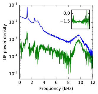
Figure 2: Representative power spectrum of a single velocity pair’s time cross correlation. The larger blue spectrum is the Hermitian component while the smaller green spectrum is the antihermitian component. The inset shows the phase of the antihermitian component at the drift frequency and has the same abscissa as the outer figure.

Drift waves also help evaluate the degree of broken symmetry of the matrix. Consider the physical set up: the periscopes shown in Fig.1 are oriented at $90^{\circ}$ to each other and each has two cones of light collection volume with concurrent tips at the focus - where the lasers are located. The drift wave amplitude peaks in the gradient region of the plasma - higher up in the cone and away from the focus. With the physical setup in mind, we quantify how the matrix symmetry can be broken. The strongest drift wave mode corresponds to the first Fourier mode decomposition $e^{im\phi}$ where $m=1$Horton (1999). We check this by separating the matrix into symmetric and antisymmetric components $S,A=\frac{1}{2}(C(v_{i},v_{j};\tau)\pm C(v_{j},v_{i};-\tau))$ and taking the Fourier transform along the time axis to acquire $\widetilde{S},\widetilde{A}$. These matrices, after this Fourier transform, are Hermitian and antihermitian by construction. Figure 2 shows a representative power spectrum from the matrix and its unwrapped phase. The unwrapped phase is $\pi/2$, and since the periscopes are positioned to have their light collection cones at angle $\pi/2$, this result is expected. The drift wave represents a worst case of broken data matrix Hermiticity, and the effect is mostly constrained in frequency space to the region around $f^{*}\approx 10$kHz as shown in Fig. 2.

Figure 2’s spectra show that the Hermiticity of the matrix remains good to at least 10 dB for nearly all frequencies lower than the drift wave. This validates our noise reduction processes for this frequency range. This also provides a second validation that the Zeeman broadening is not too large.

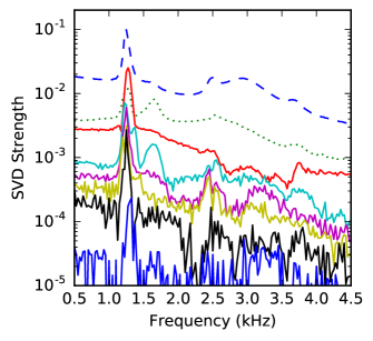
Figure 3: Power spectra from connecting the singular values of the Hermitian matrix. A separate SVD is run on each 2D velocity space and connecting the singular values across frequency gives this plot. The fact that these power spectra differ is evidence of distinct modes. The third strongest mode, in solid red, becomes second strongest around $1250\text{Hz}$ and then drops back to being third strongest. These are the velocity space degrees of freedom of plasma fluctuations as a function of frequency.

Obtaining the plasma degrees of freedom and the plasma modes is now possible. We apply a singular value decomposition (SVD)Nardone (1992)^,William H. Press William T. Vetterling Brian P. Flannery (2007) to the $2D$ Hermitian velocity matrix $\widetilde{S}$ for every point in the frequency spectrum. The SVD gives the effective rank, or detected degrees of freedom, of the matrix at a given frequency by the number of singular values above the noise level. The magnitude of each singular value determines the relative importance of its corresponding principal axis. Assuming continuity of the principal axes in frequency, we connect the singular values across the spectrum. The results are shown in Fig. 3. The strongest singular value mode spectrum is qualitatively similar to the undecomposed spectrum of Fig. 2.

However, SVD does not come without drawbacks. It assumes linearity and imposes the ansatz that the basis vectors are orthogonal. The basis of the ion velocity space distribution function may not always fulfill these assumptions. This is inextricably tied to SVD’s strength: it does not make any other assumptions about the form of these basis vectors - which is why we use it here.

For comparison with the experiment, consider electrostatic ion waves where the plasma is quasineutral and the electron density follows a Boltzmann distribution. Rewriting the linearized Vlasov equation with a Poisson bracket, expanding in the gyrophase coordinate $\varphi$ around the ion guiding centers, using a BGKBhatnagar, Gross, and Krook (1954) collision operator, and integrating over the perpendicular velocity gives

$$f_{1}(v_{||})=\sum_{n=-\infty}^{\infty}e^{-k_{\perp}^{2}v_{T}^{2}/\Omega^{2}}I_{n}(\frac{k_{\perp}^{2}v_{T}^{2}}{\Omega^{2}})\frac{n_{1}}{n_{0}}kT_{e}$$

$$\times\frac{ik_{||}\frac{\partial f_{0}}{\partial p_{||}}+(\frac{in\Omega}{kT_{\perp}}+\frac{\nu}{kT_{e}})f_{0}}{\nu+ik_{||}v_{||}-i\omega-in\Omega},$$ (2)

where $\Omega$ is the ion cyclotron frequency, $I_{n}$ is the modified Bessel function of the first kind, and $\nu$ is the collision frequency. At a given frequency, then, there is a range of modes present in the plasma, each with its own $k_{\perp}$ and $k_{||}$ corresponding to an $f_{1}$ given by Eqn. 2. Similarly, in Fig. 3, SVD resolves a subset of different modes for each given frequency and so we have separated the different spatial plasma modes with a localized measurement.

We give two examples of spatial mode separation, the first without Eqn. 2 and the second with Eqn. 2. The chamber ion acoustic longitudinal bounded mode is the $\approx 1250$ Hz peak and is strong across all modes. A similar ion acoustic longitudinal mode bounded by the wire mesh grid is at $\approx 1650$ Hz and is separated by SVD into the second and fourth most important principal axes.

The principal axes of the SVD provide a way to categorize these modes via comparison with Eqn. 2. Since the matrix $\widetilde{S}$ is Hermitian, SVD reduces to an eigenvector decomposition and thus the principal axes are the complex valued eigenvectors of the ion velocity fluctuation distribution function. A set of these eigenvectors is displayed in Fig. 4 for $f=800~{}Hz$. By fitting these against Eqn. 2 evaluated with the measured plasma parameters, we can categorize these modes. The resulting vectors from this fit are overlaid with dotted Argand diagrams for the two strongest modes in Fig. 4. The second strongest mode at top right in Fig. 4 corresponds to the spatially largest mode of the plasma chamber with $\lambda_{||}=460$ cm and fits best. However, the strongest mode itself corresponds to a smaller spatial mode with $\lambda_{||}\approx 14.6$ cm and $\lambda_{\perp}\approx 1.4$ cm and does not fit as well. This is another example of spatial mode separation from a local measurement and that theory work is an avenue of future work to interpret this measurement properly.

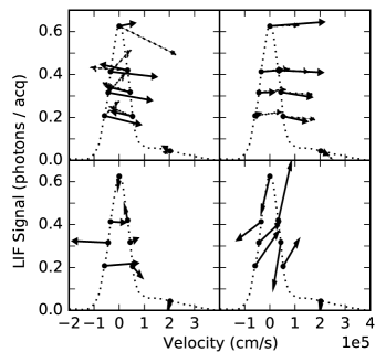
Figure 4: Eigenvectors of the four strongest singular value modes (strongest at top left and going clockwise) at $f=800$ Hz. Each vector component is complex valued and represented with a solid Argand diagram with origin at the measurement point on the deconvolved ion velocity distribution function. The Argand diagrams from Eqn. 2 are shown with dashed lines for the two strongest modes for comparison. The strongest mode’s Argand diagram describes a traditional linearized ion acoustic resonance.

These mode structures do not remain constant as a function of frequency and may also change in relative strength. By minimizing the difference in eigenvectors as frequency is varied, we can find the continuous path of evolution of eigenvectors. Thus we determine if and when the relative strength of the mode changes as a function of frequency. This process shows, for example, that the second and third modes in Fig. 3 switch in strength near $1250$ Hz.

We introduce a generalized wave admittance by normalizing the appropriate eigenmode. In the case of the ion acoustic wave, combining the linearized force balance equation with the ion acoustic wave dispersion relation gives

$$\frac{n_{0}v_{z}}{n}=c_{s}\sqrt{k_{\perp}^{2}\frac{c_{s}^{2}}{\Omega^{2}-\widetilde{\omega^{2}}}+\frac{\omega}{\widetilde{\omega}}}$$ (3)

where $\widetilde{\omega}=\omega-i\nu$. The left hand side can be calculated for each eigenmode by integrating the eigenvector to find the denominator $n$ and the eigenvector’s first velocity moment to find the numerator $n_{0}v_{z}$. Figure 5 shows these admittances calculated using the two strongest data eigenmodes normalized to the ion acoustic speed $c_{s}$.

The admittances of Fig. 5 show that the second mode, which corresponds to modes constrained by the wire mesh grid, grows to reflect the larger $k_{\perp}$. The peak in the first mode corresponds to the plasma chamber bounded mode.

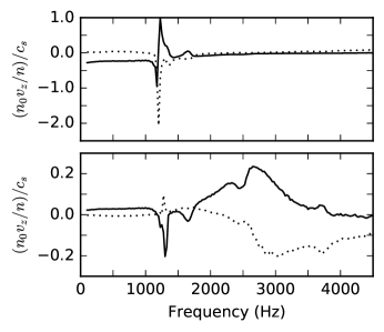
Figure 5: Normalized admittance of the eigenmodes as a function of frequency. Top is the strongest eigenmode while bottom is the second strongest eigenmode. The real component is the solid line while the imaginary is the dotted line.

To summarize, we have introduced a new method for measuring the degrees of freedom and corresponding eigenmodes of plasma ion velocity distribution function fluctuations. This method uses a singular value decomposition in order to acquire the rank and the eigenmodes, in the case of a square Hermitian matrix, or the principal axes more generally. We show that this particular localized measurement gives the discrete set of modes, both bounded modes and kinetic modes, that constitute the plasma fluctuations. Analysis shows how these modes change in strength as a function of frequency. We also calculate a generalized wave admittance for each one of these eigenmodes.

The velocity space correlation function of the plasma distribution function given by this method makes it possible to measure phase space fluctuation spectra in terms of canonical velocity coordinates. Refinement of this method will be necessary since an integral transform to this end requires a nontrivial kernel Morrison (1994). A suggestive example is recent theoretical work finding phase space density fluctuation spectra and electric field spectra Morrison and Shadwick (2008). Alternatively, it should be possible to project the data matrix onto the basis of kinetic eigenmodes, which form a complete discrete spectrum for fluctuations in a weakly collisional plasma Ng, Bhattacharjee, and Skiff (2004).

This work is supported by the US DOE under the NSF-DOE program with grant number DE-FG02-99ER54543.

References

- Van Kampen (1955) N. G. Van Kampen, Physica 21, 949 (1955).
- Case (1959) K. M. Case, Phys. Fluids 21, 249 (1959).
- Ng, Bhattacharjee, and Skiff (2004) C. S. Ng, A. Bhattacharjee, and F. Skiff, Phys. Rev. Lett. 92, 065002 (2004).
- Skiff et al. (2002) F. Skiff, H. Gunell, A. Bhattacharjee, C. S. Ng, and W. A. Noonan, Phys. Plasmas 9, 1931 (2002).
- De Souza-Machado, Sarfaty, and Skiff (1999) S. De Souza-Machado, M. Sarfaty, and F. Skiff, Phys. Plasmas 6, 2323 (1999).
- Diallo and Skiff (2005) A. Diallo and F. Skiff, Phys. Plasmas 12, 110701 (2005).
- Hatch et al. (2011) D. R. Hatch, P. W. Terry, F. Jenko, F. Merz, and W. M. Nevins, Phys. Rev. Lett. 106, 115003 (2011).
- Terry, Baver, and Gupta (2006) P. W. Terry, D. A. Baver, and S. Gupta, Phys. Plasmas 13 (2006), 10.1063/1.2168453.
- Terry et al. (2014) P. W. Terry, K. D. Makwana, M. J. Pueschel, D. R. Hatch, F. Jenko, and F. Merz, Phys. Plasmas 21 (2014), 10.1063/1.4903207.
- Stern and Johnson (1975) R. A. Stern and J. A. Johnson, Phys. Rev. Lett. 34, 1548 (1975).
- Fasoli, Skiff, and Tran (1994) A. Fasoli, F. Skiff, and M. Q. Tran, Phys. Plasmas 1, 1452 (1994).
- Uzun-Kaymak and Skiff (2006) I. Ü. Uzun-Kaymak and F. Skiff, Phys. Plasmas 13, 112108 (2006).
- Anderegg et al. (1997) F. Anderegg, X.-P. Huang, E. Sarid, and C. F. Driscoll, Rev. Sci. Instrum. 68, 2367 (1997).
- Strickler et al. (2016) T. S. Strickler, T. K. Langin, P. McQuillen, J. Daligault, and T. C. Killian, Phys. Rev. X 021021, 1 (2016), arXiv:1512.02288 .
- Sarfaty, De Souza-Machado, and Skiff (1998) M. Sarfaty, S. De Souza-Machado, and F. Skiff, Phys. Rev. Lett. 80, 3252 (1998).
- Skiff et al. (2000) F. Skiff, C. S. Ng, A. Bhattacharjee, W. A. Noonan, and A. Case, Plasma Phys. Control. Fusion 42, B27 (2000).
- Horton (1999) W. Horton, Rev. Mod. Phys. 71, 735 (1999).
- Nardone (1992) C. Nardone, Plasma Phys. Control. Fusion 34, 1447 (1992).
- William H. Press William T. Vetterling Brian P. Flannery (2007) S. A. T. William H. Press William T. Vetterling Brian P. Flannery, Numerical Recipes, 3rd ed. (Cambridge University Press, New York, NY USA, 2007).
- Bhatnagar, Gross, and Krook (1954) P. L. Bhatnagar, E. P. Gross, and M. Krook, Phys. Rev. 94, 511 (1954).
- Morrison (1994) P. J. Morrison, Phys. Plasmas 1, 1447 (1994).
- Morrison and Shadwick (2008) P. J. Morrison and B. A. Shadwick, Commun. Nonlinear Sci. Numer. Simul. 13, 130 (2008).