Fast computation of the principal components of genotype matrices in Julia

Abstract

Finding the largest few principal components of a matrix of genetic data is a common task in genome-wide association studies (GWASs), both for dimensionality reduction and for identifying unwanted factors of variation. We describe a simple random matrix model for matrices that arise in GWASs, showing that the singular values have a bulk behavior that obeys a Marchenko-Pastur distributed with a handful of large outliers. We also implement Golub-Kahan-Lanczos (GKL) bidiagonalization in the Julia programming language, providing thick restarting and a choice between full and partial reorthogonalization strategies to control numerical roundoff. Our implementation of GKL bidiagonalization is up to 36 times faster than software tools used commonly in genomics data analysis for computing principal components, such as EIGENSOFT and FlashPCA, which use dense LAPACK routines and randomized subspace iteration respectively.

65F15, 97N80

1 Principal components of genomics data

Personalized medicine or precision medicine is a growing movement to tailor treatments of disease to an individual’s sensitivities to treatment, allergies, or other genetic predispositions, using all available data about an individual [17]. Developers of personalized medical treatments are therefore interested in how an individual’s genome, both in isolation and within the context of the wider human population, can be used to predict desired clinical outcomes (known as comorbidities or phenotypes) [25, Ch. 8]. Genome-wide association studies (GWASs) are a new and popular technique for studying the significance of human genome data, by studying the associate genotype variation with phenotype variations in outcome variables e.g. the clinical observation of a disease.

The genome data used in GWASs are are often encoded in a matrix expressing the number of mutations from a reference genome, which we will refer to as a genotype matrix. By convention, the genotype matrix is indexed by patients (or other test subjects) on the rows and gene markers on the columns which represent some coordinate or locus within the human genome. A common example of gene markers are single nucleotide polymorphisms (SNPs), which represent gene positions with pointwise mutations of interest that express variation in the genotype across humans. Oftentimes, the explanatory data in a GWAS are simply called SNP data. Since most human cells are at most diploid, i.e. have two sets of chromosomes, the matrix elements can only be 0, 1, or 2 (or missing).

There are two major confounding sources of variation which are considered in the analysis of human genome data, each of which have significance for the spectral properties of the matrix:

Population stratification/admixing

Population stratification is the phenomenon of common genetic variation within mutually exclusive subpopulations defined along racial, ethnic or geographic divisions [35, 11]. (Admixture models relax the mutual exclusion constraint [18, 37].) In linear algebraic terms, the genotype matrix will have a low rank component with large singular values.

Cryptic relatedness

Sometimes called kinship or inbreeding, cryptic relatedness is an increase in sampling bias in the columns (human genomes) produced by having common ancestors, thus increasing the nominally observed frequency of certain mutations [45, 2]. Relatedness is usually detected and removed in a separate preprocessing step, but it is not always possible to remove fully [36]. Any remaining related samples will result in (near) linear dependencies in the rows of the genotype matrix, leading to the presence of several singular values that are very small or zero.

Principal component analysis (PCA) was historically first used as a dimensionality reduction technique to summarize the variation in the human genes and study its implications for human evolution in relation to other factors such as geography and history [29, 12, 30]. However, we will focus on the more modern use of principal components (PCs) to represent the confounding effects of population substructure in the statistical modeling of GWASs [13, 33, 34, 51, 50].

Genomics matrices form an interesting use case for the classical techniques of numerical linear algebra, as the amount of sequenced genome data grows exponentially [40]. As the price of sequencing genome data declines rapidly, genomics studies involving hundreds of thousands of individuals (columns) are already commonplace today, with order of magnitude growth expected within the next year or two. Therefore, genomics researchers will require access to the best available algorithms for parallel computing and numerical linear algebra to handle the increasing demands of data processing and dimensionality reduction.

1.1 The statistical significance of principal components

The main statistical tool used in GWAS is regression, using some model that associates genotype variation with phenotype variation. While correlation does not imply causation in and of itself, the central dogma of molecular biology states that causality flows from genetic data in DNA and RNA to phenotype data in expressed proteins [14]. Consequently, correlations between genotypes and phenotypes could in theory have causal significance. The linear regression model is one the simplest useful models, and can be motivated in several different ways. One way is in terms of least squares minimization to find the coefficients that minimize the sum of squared distances between a hyperplane and the observations. Another way to formulate the problem as finding a projection of the vector of observations down onto the space spanned by the vectors of explanatory variables. One caveat in statistical studies is the assumption that the observations are randomly sampled with replacement, and hence that the observations can be assumed to be independent. In the context of statistical genomics, the independence assumption is one of several bundled into the principle of Hardy-Weinberg equilibrium [23, 46], which is commonly assumed in statistical genetics [25]. However, caution must be taken to remove possible sampling bias due to the collection of genetic data from patients from a single hospital or hospital network, on top of sampling bias introduced by not treating the presence of population substructure.

1.2 The linear regression model

The statistical theory of regressing phenotypes against genotypes is best expressed in terms from conditional expectations. If we for individual $i$ denote the genotype measurement by $x_{i}$ and the phenotype measurement by $y_{i}$, the conditional expectation of interest can be written as $\operatorname{E}(y_{i}|x_{i})=\beta_{0}+\beta_{1}x_{i}$. A popular formulation of the this model is

$$y_{i}=\beta_{0}+x_{i}\beta_{1}+\varepsilon_{i}\quad i=1,\dots,n$$

where $n$ is the number of observations which in this case would be the number of individuals for which we have genotype data. The variable $\varepsilon_{i}$ is called the error term and must satisfy $\operatorname{E}(\varepsilon_{i}|x_{i})=0$. More generally, $\varepsilon_{i}$ is the conditional distribution $y_{i}-\beta_{0}-x_{i}\beta_{1}|x_{i}$.

The multivariate expression can be written conveniently in matrix form

(1) $$y=X\beta+\varepsilon$$

with

$$X=\begin{pmatrix}1&x_{1}\\ \vdots&\vdots\\ 1&x_{n}\end{pmatrix}$$

and in this notation, the well-known least squares estimator for the coefficient $\beta$ can be written as

(2) $$\hat{\beta}=(X^{T}X)^{-1}X^{T}y.$$

The conditional probability treatment demonstrates that when $(x_{i},y_{i})$ pairs are considered to be random variables, then $\hat{\beta}$ is also a random variable, with its mean and variance quantifying uncertainty about the least squares solution. First, notice that the least squares estimator (2) can be written

$$\hat{\beta}=\beta+(X^{T}X)^{-1}X^{T}\varepsilon$$

and the expected value of the estimator is

(3) $$\operatorname{E}(\hat{\beta}|X)=\operatorname{E}(\beta+(X^{T}X)^{-1}X^{T}\varepsilon|X)=\beta+(X^{T}X)^{-1}X^{T}\operatorname{E}(\varepsilon|X)=\beta$$

which means that the estimator is unbiased. Statisticians are interested in the variability of $\hat{\beta}$ under changes to the data that could be considered small errors. The most common measurement for the variability of an estimator is the (conditional) variance, i.e.

$$\operatorname{Var}(\hat{\beta}|X)=\operatorname{Var}(\beta+(X^{T}X)^{-1}X^{T}\varepsilon|X)=(X^{T}X)^{-1}X^{T}\operatorname{Var}(\varepsilon|X)X(X^{T}X)^{-1}.$$

This shows that variance of $\hat{\beta}$ depends on the (conditional) variance of $\varepsilon$, which has not been discussed yet. In classical treatments of the linear regression model it is typically assumed that, conditionally on $x_{i}$, the $y_{i}$s are independent and the have the same variance which is the same as $\operatorname{Var}(\varepsilon|X)=\sigma^{2}I$ for some unknown scalar $\sigma^{2}$. Under this assumption, the variance of $\hat{\beta}$ reduces to $\sigma^{2}(X^{T}X)^{-1}$. The magnitude of this quantity is unknown because $\sigma^{2}$ is an unknown parameter but $\sigma^{2}$ can be estimated from the data. The usual estimator is $\hat{\sigma}^{2}=\frac{1}{n}\|\hat{\varepsilon}\|^{2}$ where $\hat{\varepsilon}=y-X\hat{\beta}$. This leads to the estimate of the (conditional) variance of the estimator $\widehat{\operatorname{Var}(\hat{\beta}|X)}=\hat{\sigma}^{2}(X^{T}X)^{-1}$.

The independence assumption is often used in statistics and can be justified from an assumption of random sampling with replacement. In studies where data is passively collected, this might not be a reasonable assumption as explained in the previous section. Non-random sampling might lead to correlation between the phenotypes even after conditioning on the genotypes. In consequence of that, $\operatorname{Var}(\varepsilon|X)$ will no longer be diagonal, but have some general positive definite structure $\Sigma$ and $\operatorname{Var}(\hat{\beta}|X)=(X^{T}X)^{-1}X^{T}\Sigma X(X^{T}X)^{-1}$. Since $\Sigma$ in general consists of $\frac{n(n+1)}{2}$ parameters, it cannot be estimated consistently.

In order to analyze the problem with correlated observations, it is convenient to decompose the error into a part that contains the cross-individual correlation and a part that is diagonal and therefore only describes the variance for each individual. This may be written as

$$y_{i}=\beta_{0}+x_{i}\beta_{1}+\eta_{i}+\xi_{i}$$

where is assumed that $\operatorname{Var}(\eta|X)=\Sigma_{\eta}$ and $\operatorname{Var}(\xi|X)=\sigma^{2}_{\xi}I$. Furthermore, it is assumes that the two error terms are independent.

1.2.1 Fixed effect estimation

One way to produce a reliable estimate of the variance of $\hat{\beta}$ is to come up with a set of variables $z_{1},\dots,z_{k}$ that proxies the correlation between the observations, i.e. $\eta=Z\gamma$. By simply including the variables $z_{1},\dots,z_{k}$ in the regression model, it possible to remove the correlation which distorts the variance estimate for $\hat{\beta}$. For the regression $y|X,Z$, we get the least squares estimator

$$\begin{pmatrix}\hat{\beta}\\ \hat{\gamma}\end{pmatrix}=\begin{pmatrix}X^{T}X&X^{T}Z\\ Z^{T}X&Z^{T}Z\end{pmatrix}^{-1}\!\!\begin{pmatrix}X^{T}\\ Z^{T}\end{pmatrix}(X\beta+Z\gamma+\xi)=\theta+\begin{pmatrix}X^{T}X&X^{T}Z\\ Z^{T}X&Z^{T}Z\end{pmatrix}^{-1}\!\!\begin{pmatrix}X^{T}\\ Z^{T}\end{pmatrix}\xi,$$

which has variance

$$\operatorname{Var}\left(\begin{pmatrix}\hat{\beta}\\ \hat{\gamma}\end{pmatrix}|X,Z\right)=\sigma_{\xi}^{2}\begin{pmatrix}X^{T}X&X^{T}Z\\ Z^{T}X&Z^{T}Z\end{pmatrix}^{-1}.$$

In many applications, a few principal components of the covariance matrix of the complete SNP data set is used as a proxy for the correlation between individuals. Computing principal components is therefore often a first step in analyzing GWASs.

1.3 Software for computing the principal components of genomics data

The software stack for GWAS is generally based on command line tools written completely in C/C++. Not only is the core computational algorithm written in C/C++ but also much of the pre- and postprocessing of the data. The data sets can be large but and the computations at times heavy but it has been a surprise to learn the extend to which analyses are carried out directly from the command line instead of using higher level languages like MATLAB, R, or Python. This choice seems to limit the tools available to the analysts because, unless he is a C/C++ programmer, the programmer is restricted to the set of options included in the command line tool.

Two major packages exist for computing the PCA in the GWAS software stack. The package EIGENSOFT accompanied [33] which popularized the use of PCA in GWAS. In the original version of the package, the routine smartpca for computing the PCA of a SNP matrix was based on an eigenvalue solver from LAPACK. In consequence, all the eigenvalues and vectors of the SNP matrix were computed even though only a few of them were used as principal components. Computing the full decomposition is inefficient and as the number of available samples has grown over the year, this approach has become impractical.

More recently, FlashPCA [1] has emerged as a potentially faster alternative to EIGENSOFT’s smartpca. The PCA routine is based on a truncated SVD algorithm described in [22]. More specifically, FlashPCA uses a subspace iteration scheme with either column-wise scaling (FlashPCA 1) or orthogonalization by QR (FlashPCA 2) in each iteration. The convergence criterion is based on the average of squared element-wise distance between the the bases for iteration $i-1$ and $i$. The QR orthogonalization step in the implementation of FlashPCA routine deviates from the algorithm in described [1] which only normalizes column-wise. Our conjecture was that this change was made to avoid loss of orthogonality in the subspace basis and the author of the package has confirmed this. In consequence, the timings in [1] do not correspond to the performance of the software run with default settings since the QR orthogonalization is much slower than the column-wise normalization. Furthermore, a degenerate basis might also converge much faster because it eventually converges to the single largest eigenvalue.

Table 1 lists some software packages providing eigenvalue or singular value computations useful for PCA. It may surprise readers that well-established packages in numerical linear algebra are rarely used in genomics, considering that libraries like ARPACK and PROPACK have convenient wrapper libraries in both R, Python, and MATLAB. This phenomenon might be explained by the pronounced use of C/C++ in statistical genetics, where calling ARPACK and PROPACK are relatively more demanding, combined with the fact that iterative methods are traditionally not part of the curriculum in statistical genomics.

Table 1: List of software used for principal components analysis in statistical genomics. Notably, common packages known to numerical linear algebraists are rarely, if ever, used. ^∗: available in EIGENSOFT [33]. ^†: uses dense LAPACK routines.

Software	Reference	Algorithm	Used in genomics
smartpca∗†	[33]	Householder bidiagonalization	✓
FastPCA∗	[19]	Subspace iteration	✓
FlashPCA	[1]	Subspace iteration	✓
ARPACK	[27]	Lanczos tridiagonalization	✗
PROPACK	[26]	Lanczos bidiagonalization	✗
SLEPc	[24]	Lanczos bidiagonalization	✗
Anasazi	[6]	Lanczos bidiagonalization	✗

2 A simple model for genomics data

In this section we present a very simple random model which accurately mimics the spectral features observed in real data matrices. We hypothesize that the spectral properties of human patient genotype data can be modeled the Julia code in Algorithm 1, which captures the confounding effects of population admixture and cryptic relatedness. The former is modeled by setting randomly select subblocks to the same value, whereas the latter is modeled by duplicating rows, thus purposely introducing linear dependence into the row space. This model, while simplistic, can be tuned to reproduce the scree plot observed in empirical data matrices and we expect that such models may be of interest to researchers developing numerical algorithms that lack access to actual data, which are often access-restricted due to clinical privacy.

Algorithm 1 A simple model for human genotype data matrices in Julia

⬇

1"""

2Inputs:

3- m: number of rows (gene markers)

4- n: number of columns (patients)

5- r: number of subblocks to model population admixing

6- nsignal: number of entries to represent signal

7- rkins: fraction of columns to duplicate

8

9Output:

10- A: a dense matrix of size m x n with matrix elements 0, 1 or 2

11"""

12function model(m, n, r, nsignal, rkins)

13 A = zeros(m, n)

14 #Model population admixing

15 #by randomly setting a subblock to the same value, k

16 for i=1:r

17 k = rand(0:2)

18 r1 = randrange(m)

19 r2 = randrange(n)

20 A[r1, r2] = k

21 end

22

23 #Model signal

24 for i=1:nsignal

25 A[rand(1:m), rand(1:n)] = rand(0:2)

26 end

27

28 #Model kinship by duplicating rows

29 nkins = round(Int, rkins*m)

30 for i=1:nkins

31 A[rand(1:m), :] = A[rand(1:m), :]

32 end

33 return A

34end

35

36function randrange(n)

37 i1 = rand(1:n)

38 i2 = rand(1:n)

39 if i1 > i2

40 return i2:i1

41 else

42 return i1:i2

43 end

44end

Algorithm 1 describes a model function, which creates a dense, synthetic data matrix of size $m\times n$. The synthetic data is generated in three steps. First, randomly select $r$ rectangular submatrices (which may overlap) and set the elements of each submatrix to the same value. This process simulates crudely the effects of population admixture, where each subpopulation has a common block of mutations that vary together, and the possibility of overlap resembles the effect of mixing different subpopulations together. (This step uses the auxiliary randrange function, which returns a valid Julia range that is a subinterval of the range 1:n.) Second, model the genotype of interest by randomly setting $nsignal$ matrix elements randomly to 0, 1 or 2. Third, simulate the effects of kinship by choosing a fraction $rkins$ of the rows to duplicate.

The model is clearly a very crude approximation to genotype data with the confounding effects of population substructure. There is little overt control over the admixture process, the precise distribution over matrix elements, and all related patients are assumed to have identical genotypes. Nevertheless, the model generates realistic distributions of singular values which mimic closely what we have observed in that of real world genotype matrices. Figure 1 shows the distribution of singular values generated by our model with parameters $m=41505$, $n=81700$, $r=10$, $nsignal=mn$, $rkins=0.017$. There are a handful of ($\approx r$) large singular values, while the rest follow a bulk distribution from random matrix theory known as the Marchenko-Pastur law [28] with parameter $\rho=1.86$.

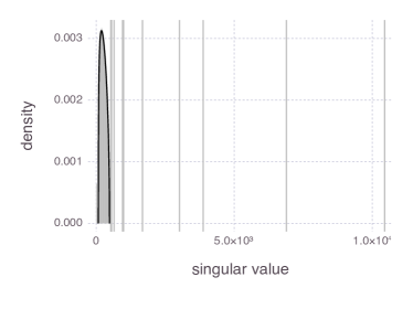
Figure 1: Left: Histogram of the singular values of a synthetic genomics data matrix of size $41505\times 81700$ (grey bars) generated with the code in Algorithm 1, overlaid with the Marchenko-Pastur law (5) for $\rho=1.86$ (black line). Light gray vertical lines show the presence of 18 outlying singular values whose magnitudes exceed $1.1\sigma_{+}\approx 529.7$. Right: Scree plot of the singular values of the same matrix (black solid lines), showing the presence of a large, low rank portion of approximately rank 10 (inset), and an asymptotic convergence to the same Marchenko-Pastur law (red dotted line).

The Marchenko-Pastur law describes the distribution of governs the eigenvalues of a random covariance matrix $Y=XX^{T}$ formed from a data matrix $X$ of iid elements with mean 0 and finite variance $\sigma^{2}$. Let $\rho$ be the ratio of the number of rows of $X$ to the number of columns of $X$. Then, the nonzero eigenvalues follow the distribution

(4) $$p_{e}(\xi)=\frac{\sqrt{(\lambda_{+}-\xi)(\xi-\lambda_{-})}}{2\pi\sigma^{2}\lambda x}$$

where $\lambda_{+}=\sigma^{2}(1+\sqrt{\rho})^{2}$ and $\lambda_{-}=\sigma^{2}(1-\sqrt{\rho})^{2}$.

When written in terms of the probability density of the singular values of $X$, the law reads

(5) $$p_{s}(x)=\frac{\sqrt{(\sigma_{+}^{2}-x^{2})(x^{2}-\sigma_{-}^{2})}}{\pi\sigma^{2}\min(1,\lambda)x}$$

where $\sigma_{+}=\sqrt{\lambda_{+}}=\sigma(1+\sqrt{\rho})$ and $\sigma_{-}=\sqrt{\lambda_{-}}=\sigma|1-\sqrt{\rho}|$.

Figure 2 shows typical density plots for random eigenvalues and singular values for $\rho=1.5$.

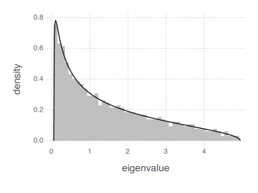
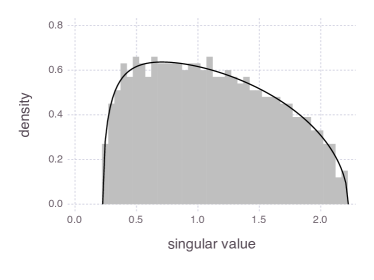
Figure 2: Marchenko-Pastur law for $\rho=1.5$ (black lines) for the densities of nonzero eigenvalues of a random covariance matrix ($XX^{T}$) and the singular values of $X$ for iid matrix elements with mean 0 and variance 1 (black lines), corresponding to (4) and (5) respectively. Shown for comparison are corresponding histograms (grey bars) of numerically sampled eigenvalues and singular vectors from a numerically sampled random matrix $X$ of size $1000\times 667$, with iid Gaussian entries of mean 0 and variance 1.

It is worth noting that random matrix theory had been previously introduced in the theoretical analysis of principal components of genotype matrices. [33] proposed a hypothesis test that computed principal components should correspond to eigenvalues that were different from those expected from a pure random covariance matrix, and comparing in particular the largest eigenvalue against one randomly sampled from the Tracy-Widom distribution [44, 43]. This analysis only shows that the matrix is not iid. In contrast, we show here an explicit construction of a random matrix, whose elements are not iid, that can generate a realistic spectrum of singular values that consists of several large outliers and a bulk distribution that empirically satisfies the Marchenko-Pastur law, albeit with a modified parameter $\rho=1.86$ as opposed to the value $81700/41505=1.97$ which would be expected from taking the ratio of the number of rows to the number of columns.

3 Algorithms for PCA

The discussion in Section 1 demonstrates that the confounding effects of population substructure can and does produce a low rank structure in the top singular vectors (i.e. singular triples corresponding to the largest singular values), which can be captured even in the very crude random matrix model of Algorithm 1. The top few principal components, which by construction capture the largest components of the variability, are good candidates for modeling the unwanted variation as described in Section 1.2 and have been used in the statistical genetics community for this purpose [13, 33, 34, 51, 50].

Iterative eigenvalue (or singular value) methods [5] are therefore computationally efficient choices for determining these principal components, as only a handful of them are needed. However, none of the classical methods known in numerical linear algebra (apart from subspace iteration) is implemented in commonly used software packages for PCAs in genomics, as shown in Table 1. Notably absent is any Lanczos-based bidiagonalization method. We have therefore implemented the Golub-Kahan-Lanczos bidiagonalization [21] method in pure Julia[8, 9]. We have incorporated several of the best available numerical features, such as:

Thick restarting

To control the memory usage and accumulation of roundoff error, we also include an implementation of the thick restart strategy [48, 41], offering restarts using either ordinary Ritz values [48] or harmonic Ritz values [3]. The thick restart variant is becoming increasingly popular, being available not only in SLEPc [24], but also in R as the IRLBA package [4], and has also become the new algorithm for svds in MATLAB R2016a (which also offers partial reorthogonalization) [42]. For the purposes of computing the top principal components, it suffices to use thick restarts using ordinary Ritz values.

Choice of reorthogonalization strategy

We offer users the choice of partial reorthogonalization [38, 26] or full reorthogonalization using doubly reorthogonalized classical Gram-Schmidt. By default, the implementation uses an adaptive threshold for determining when the second reorthogonalization is necessary, based on the expected number of digits lost to catastrophic cancellation [15, 10]. We also use the adaptive one-sided reorthogonalization strategy on either the left or right singular vectors (whichever is smaller), unless our estimate of the matrix norm is sufficiently large so that two-sided reorthogonalization is necessary [39].

Convergence criteria

We use several different tests for determining when a Ritz value has converged. At the beginning of the calculation when no other information is known about the Ritz values, we use the crude estimate on the absolute error bound on the singular values based on the residual norm computed from a candidate Ritz value-vector pair [47, Ch. 3, §53, p. 70]. However, when the Ritz values become sufficiently well-separated, more refined estimates can be derived from the Rayleigh-Ritz properties of the Krylov process [47, Ch. 3, §54-55, p. 73][49, 31]. Experimental facilities are also provided to print and inspect further convergence information, such as Yamamoto’s eigenvector error bounds [49], Geurt’s formula for the componentwise backward error [20], Deif’s results for a posteriori bounds on eigenpairs and their backward error [16]. Interested users and developers can easily modify the code to implement and inspect yet other other proposed termination criteria [7].

The implementation of Lanczos bidiagonalization in Julia allows us to introspect in great detail into the inner workings of the algorithm. Figures 3 and 4 show two different sets of running parameters for our code. The former is run with no restarting and partial reorthogonalization with threshold $\omega=10^{-8}$, whereas the latter uses full reorthogonalization with thick restarting with a maximum subspace size of 40.

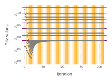
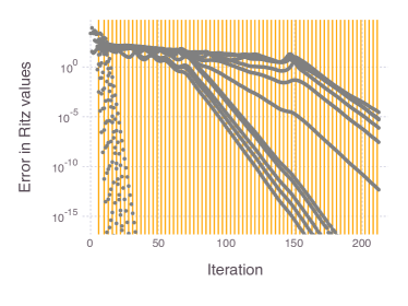
Figure 3: Golub-Kahan-Lanczos bidiagonalization in Julia with no restarting and partial reorthogonalization at a threshold of $\omega=10^{-8}$, requesting the top 20 singular values only. Orange vertical lines show when reorthogonalization was triggered in the computation. Left: Convergence behavior of the Ritz values. Right: Computed errors in Ritz values from the residual norm criterion.

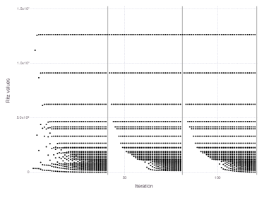
Figure 4: Golub-Kahan-Lanczos bidiagonalization in Julia with thick restarting every 40 microiterations and full reorthogonalization, requesting the top 20 singular values only. Gray vertical lines show when restarting was triggered in the computation.

3.1 Convergence analysis of subspace iteration

The software in Table 1 rely heavily on randomized block power interactions, which are essentially equivalent to subspace iteration with a randomized starting subspace.

FlashPCA also uses an unconventional convergence criterion, namely the matrix norm of the difference between successive subspace basis vectors,

(6) $$\Delta Y_{n}=\|Y_{n}-Y_{n-1}\|.$$

A simple check of the condition number of $Y_{n}$ with block iteration $n$ shows that the basis produced by the published version of FlashPCA (which does not reorthogonalize the basis vectors) rapidly leads to a linearly dependent set of vectors. As shown in Figure 5, the loss of linear dependence occurs essentially exponentially, with the inverse condition number reaching machine epsilon after just five block iterations. Therefore, we do not recommend the published version of the FlashPCA algorithm for finding principal components, as it is practically guaranteed to not find all the principal components requested. We note that the current version of FlashPCA, which is newer than the published version, reorthogonalizes the basis vectors by default. In this paper, we refer to the older and newer versions as FlashPCA 1 and 2 respectively, to avoid ambiguity.

Figure 5: Condition number of the matrix of subspace basis per iteration for the published version of FlashPCA [1], which normalizes each vector but does not reorthogonalize them. Iteration zero is computed for the normalized basis after the initial range computation.

4 Performance and accuracy of Lanczos vs. subspace iteration

We compared FlashPCA and our code on a machine with 230 GB of RAM and two Intel(R) Xeon(R) CPU E5-2697 v2 @ 2.70GHz processors, each with 12 cores. We used the FlashPCA v1.2 release binary for Linux. Our Julia code was run on a pre-release v0.5 version of Julia, built with Intel Composer XE 2016.0.109 Linux edition, and linked against Intel’s Math Kernel Library v11.3.

Table 2 shows a breakdown of the execution time in FlashPCA compared to our Lanczos implementation on our synthetic genotype matrix. We observe a large difference in the run time between our Lanczos implementation and subspace iteration. The bulk of the difference comes from Lanczos taking much fewer iterations (as measured by matrix-vector products) to converge. For FlashPCA, most of the run time is spent in an initial matrix multiply, $XX^{T}$, and the subsequent subspace iterations.

Table 2: Run time in seconds for a synthetic genotype matrix of size $41505\times 81700$ generated using Algorithm 1. FlashPCA 1: the published version of the FlashPCA program algorithm [1], which normalizes but does not reorthogonalizes the vectors. FlashPCA 2: the current version of the FlashPCA program, which now by default normalizes and reorthogonalizes the vectors using dense QR factorization. This work: Golub-Kahan-Lanczos bidiagonalization without restarting, employing partial reorthogonalization.

	FlashPCA 1	FlashPCA 2	this work
Preprocessing	54	61	54
Forming $XX^{T}$	971	926	N/A
Subspace/Lanczos iteration	41	1935	37
Postprocessing	7	11	0
Total	1073	2933	81

Forming the matrix $XX^{T}$ is the default option in FlashPCA; while advantageous for very wide matrices $\rho\approx 0$, it is an expensive step for our matrix, which has $\rho\approx 2$. Furthermore, we observe a performance penalty in using the Eigen linear algebra library (used by FlashPCA) relative to MKL. Whereas the former took 926 seconds to compute $XX^{T}$, the latter took only 306 seconds on the same machine, using the same number of threads. This discrepancy may be system dependent.

The subspace iterations form the bulk of the run time for FlashPCA 2. Even when doing explicit reorthogonalization of the basis vectors, FlashPCA still performs many more matrix-vector product-equivalents than our Lanczos implementation with no restarting and partial reorthogonalization. Figure 6 contrasts the convergence reported by FlashPCA 2 and our Lanczos implementation. Note that the convergence criteria used by the two programs are very different—the former uses the criterion (6), which is very different from the classical residual norm criteria commonly used by Lanczos-based methods [32]. Convergence of FlashPCA 2 is very slow, being nearly stagnant for many iterations before improving dramatically in the last iteration. In contrast, the Lanczos-based method shows essentially logarithmic convergence in the residual norm after the first few iterations.

(a) FlashPCA 2

(b) this work

Figure 6: Convergence of the FlashPCA 2 and Lanczos-based algorithms. The convergence criterion used in FlashPCA 2 is (6), which in principle can be very different from the residual norm criterion used in our Lanczos-based implementation. Convergence of FlashPCA 2 is very slow, being nearly stagnant for many iterations before improving dramatically in the last iteration. In contrast, the Lanczos-based method shows essentially logarithmic convergence in the residual norm after the first few iterations.

Finally, we compare in Table 3 the relative performance and accuracy of the subspace iteration methods against our Lanczos implementations as well as two other established libraries, ARPACK [27] and PROPACK [26]. ARPACK, while not originally designed for singular value computations, can be used to compute eigenvalues of the augmented matrix $\begin{pmatrix}0&X\\ X^{T}&0\end{pmatrix}$, whose eigenvalues are the same as the singular values of $X$. To measure performance, we count the number of matrix-vector product (mvps) as well as the wall time using the threaded BLAS implementation of MKL on 24 threads. To measure accuracy, we provide both $\|\Delta\theta\|_{1}=\sum_{j=1}^{k}\beta_{n}|U^{(n)}_{mj}|$, the sum of all estimated errors for the singular values, as well as the relative error of the 10th singular value as computed by LAPACK. Our results show that our implementation of Lanczos bidiagonalization provides qualitatively better singular values that the subspace iteration methods provided by FlashPCA, even with QR reorthogonalization. Furthermore, our performance is significantly better than the standard tools, ARPACK and PROPACK.

	Algorithm	mvps	time (sec)	$\left\|\Delta\theta\right\|_{1}$	rel. err.
FlashPCA1	Block power	800	1073	$2.55$	$0.067$
FlashPCA2	Block power	33600	2933	$0.0146$	$1.88\cdot 10^{-5}$
PROPACK	GKL (PRO, NR)	N/A	120	$5.2\cdot 10^{-5}$	$1.75\cdot 10^{-11}$
ARPACK	GKL (FRO, IR)	338	378	$9.2\cdot 10^{-6}$	$8.34\cdot 10^{-15}$
this work	GKL (FRO, TR)	360	132	$0.0037$	$5.03\cdot 10^{-8}$
this work	GKL (PRO, NR)	190	81	$2.5\cdot 10^{-6}$	$1.16\cdot 10^{-14}$

Table 3: Comparing various methods for computing the top 10 principal components on a simulated genotype matrix of size $41505\times 81700$. Linear algebra kernels were run on MKL with 24 software threads except for FlashPCA which ran on Eigen kernel. Timings reported are wall times in seconds. FlashPCA1 - FlashPCA with columnwise rescaling, FlashPCA2 - FlashPCA with QR orthogonalization, GKL - Golub–Kahan–Lanczos bidiagonalization, PRO - partial reorthogonalization, FRO - full reorthogonalization, NR - no restart, IR - implicit restart after 20 Lanczos vectors, TR - thick restart after 20 Lanczos vectors, mvps - number of matrix–vector products. Termination criterion set to $\|\Delta Y\|=10^{-8}$ for FlashPCA$n$, and relative error in the 10th singular value compared with the value obtained from LAPACK.

5 Conclusions

GWASs provide an exciting new data source for large scale matrix computations, whose nominal dimensions are already on the order of $10^{5}\times 10^{5}$ and will continue to grow rapidly in the near future. The statistical and computational demands of GWAS on genotype matrices necessitate the best numerical algorithms and software.

We have implemented state of the art Lanczos bidiagonalization methods in pure Julia, allowing us to compute the largest principal components of genotype matrices more efficiently than any other tool currently being used for genomics data analysis, and even outperforming some standard packages for iterative eigenvalue and singular value computation such as ARPACK and PROPACK. The implementation of these methods in the Julia programming language provides a fast, practical software tool that permits easy introspection into the inner workings of the Lanczos algorithms, as well as experimentation into new methods with minimal fuss.

Further work may include generalizing the code to also handle block Lanczos computations, which may further improve the performance of the computation by making use of BLAS3 function calls. Imputation of missing data will also become important in future data analysis, as nominal matrix sizes grow and the number of incorrectly sequenced sites grows. We are also implementing and studying into iterative methods for evaluating the regression models used in GWASs.

References

- [1] G. Abraham and M. Inouye, Fast principal component analysis of large-scale genome-wide data, PloS One, 9 (2014), p. e93766, doi:10.1371/journal.pone.0093766.
- [2] W. Astle and D. J. Balding, Population structure and cryptic relatedness in genetic association studies, Statistical Science, 24 (2009), pp. 451–471, doi:10.1214/09-STS307.
- [3] J. Baglama and L. Reichel, Augmented implicitly restarted lanczos bidiagonalization methods, SIAM Journal on Scientific Computing, 27 (2005), pp. 19–42, doi:10.1137/04060593X.
- [4] J. Baglama, L. Reichel, and B. W. Lewis, irlba: Fast truncated SVD, PCA and symmetric eigendecomposition for large dense and sparse matrices, 2016, https://cran.r-project.org/web/packages/irlba.
- [5] Z. Bai, T.-Y. Chen, D. Day, J. W. Demmel, J. J. Dongarra, A. Edelman, R. W. Freund, M. Gu, B. Kgström, A. Knyazev, P. Koev, T. Kowalski, R. B. Lehoucq, R.-C. Li, X. S. Li, R. Lippert, K. Maschhoff, K. Meerbergen, R. Morgan, A. Ruhe, Y. Saad, G. L. G. Sleijpen, D. C. Sorensen, and H. A. van der Vorst, Templates for the Solution of Algebraic Eigenvalue Problems: A Practical Guide, Software, Environments, Tools, SIAM, Philadelphia, PA, 2000, doi:10.1137/1.9780898719581.
- [6] C. G. Baker, U. L. Hetmaniuk, R. B. Lehoucq, and H. K. Thornquist, Anasazi software for the numerical solution of large-scale eigenvalue problems, ACM Transactions on Mathematical Software, 36 (2009), p. 13, doi:10.1145/1527286.1527287.
- [7] M. Bennani and T. Braconnier, Stopping criteria for eigensolvers, Tech. Report TR/PA/94/22, CERFACS, 1994.
- [8] J. W. Bezanson, Julia: an efficient dynamic language for technical computing, S.M., Massachusetts Institute of Technology, 2012, http://18.7.29.232/handle/1721.1/74897.
- [9] J. W. Bezanson, Abstractions in Technical Computing, Ph.D., Massachusetts Institute of Technology, 2015, https://github.com/JeffBezanson/phdthesis.
- [10] Å. Björck, Numerical Methods in Matrix Computations, Texts in Applied Mathematics, Springer, 2015, doi:10.1007/978-3-319-05089-8.
- [11] L. R. Cardon and L. J. Palmer, Population stratification and spurious allelic association, The Lancet, 361 (2003), pp. 598 – 604, doi:10.1016/S0140-6736(03)12520-2.
- [12] L. L. Cavalli-Sforza, P. Menozzi, and A. Piazza, The history and geography of human genes, Princeton University Press, Princeton, NJ, 1994.
- [13] H.-S. Chen, X. Zhu, H. Zhao, and S. Zhang, Qualitative semi-parametric test for genetic associations in case-control designs under structured populations, Annals of Human Genetics, 67 (2003), pp. 250–264, doi:10.1046/j.1469-1809.2003.00036.x.
- [14] F. H. C. Crick, Central dogma of molecular biology, Nature, 227 (1970), pp. 561–563, doi:10.1038/227561a0.
- [15] J. W. Daniel, W. B. Gragg, L. Kaufman, and G. W. Stewart, Reorthogonalization and stable algorithms for updating the Gram-Schmidt QR factorization, Mathematics of Computation, 30 (1976), pp. 772–795, doi:10.1090/S0025-5718-1976-0431641-8.
- [16] A. Deif, A relative backward perturbation theorem for the eigenvalue problem, Numerische Mathematik, 56 (1989), pp. 625–626, doi:10.1007/BF01396348.
- [17] S. Desmond-Hellmann, Toward precision medicine: A new social contract?, Science Translational Medicine, 4 (2012), pp. 129ed3–129ed3, doi:10.1126/scitranslmed.3003473.
- [18] B. Devlin and K. Roeder, Genomic control for association studies, Biometrics, 55 (1999), pp. 997–1004, http://www.jstor.org/stable/2533712.
- [19] K. Galinsky, G. Bhatia, P.-R. Loh, S. Georgiev, S. Mukherjee, N. Patterson, and A. Price, Fast principal-component analysis reveals convergent evolution of ADH1B in Europe and East Asia, The American Journal of Human Genetics, 98 (2016), pp. 456–472, doi:10.1016/j.ajhg.2015.12.022.
- [20] A. J. Geurts, A contribution to the theory of condition, Numerische Mathematik, 39 (1982), pp. 85–96, doi:10.1007/BF01399313.
- [21] G. Golub and W. Kahan, Calculating the singular values and pseudo-inverse of a matrix, Journal of the Society for Industrial and Applied Mathematics Series B Numerical Analysis, 2 (1965), pp. 205–224, doi:10.1137/0702016.
- [22] N. Halko, P.-G. Martinsson, and J. A. Tropp, Finding structure with randomness: Probabilistic algorithms for constructing approximate matrix decompositions, SIAM review, 53 (2011), pp. 217–288, doi:10.1137/090771806.
- [23] G. H. Hardy, Mendelian proportions in a mixed population, Science, 28 (1908), pp. 49–50, doi:10.1126/science.28.706.49.
- [24] V. Hernández, J. E. Román, and A. Tomás, A robust and efficient parallel SVD solver based on restarted Lanczos bidiagonalization, Electronic Transactions on Numerical Analysis, 31 (2008), pp. 68–85, http://etna.mcs.kent.edu/volumes/2001-2010/vol31/abstract.php?vol=31%5C&pages=68-85.
- [25] N. M. Laird and C. Lange, The Fundamentals of Modern Statistical Genetics, Statistics for Biology and Health, Springer, New York, 2011, doi:10.1007/978-1-4419-7338-2.
- [26] R. M. Larsen, Lanczos bidiagonalization with partial reorthogonalization, PhD thesis, Aarhus, 1998, http://soi.stanford.edu/~rmunk/PROPACK/.
- [27] R. B. Lehoucq and D. C. Sorensen, Deflation techniques for an implicitly restarted Arnoldi iteration, SIAM Journal on Matrix Analysis and Applications, 17 (1996), pp. 789–821, doi:10.1137/S0895479895281484.
- [28] V. A. Marčenko and L. A. Pastur, Distribution of eigenvalues for some sets of random matrices, Mathematics of the USSR-Sbornik, 1 (1967), p. 457, http://stacks.iop.org/0025-5734/1/i=4/a=A01.
- [29] P. Menozzi, A. Piazza, and L. Cavalli-Sforza, Synthetic maps of human gene frequencies in europeans, Science, 201 (1978), pp. 786–792, doi:10.1126/science.356262.
- [30] J. Novembre and M. Stephens, Interpreting principal component analyses of spatial population genetic variation, Nature Genetics, 40 (2008), pp. 646–649, doi:10.1038/ng.139.
- [31] J. M. Ortega, Numerical Analysis: A Second Course, Classics in Applied Mathematics, SIAM, Philadelphia, PA, 2 ed., 1990, doi:10.1137/1.9781611971323, http://epubs.siam.org/doi/book/10.1137/1.9781611971323.
- [32] B. N. Parlett, The Symmetric Eigenvalue Problem, Classics in Applied Mathematics, SIAM, Philadelphia, PA, 2 ed., 1998, doi:10.1137/1.9781611971163.
- [33] N. Patterson, A. L. Price, and D. Reich, Population structure and eigenanalysis, PLoS Genetics, 2 (2006), p. e190, doi:10.1371/journal.pgen.0020190.
- [34] A. L. Price, N. J. Patterson, R. M. Plenge, M. E. Weinblatt, N. A. Shadick, and D. Reich, Principal components analysis corrects for stratification in genome-wide association studies, Nature Genetics, 38 (2006), pp. 904–909, doi:10.1038/ng1847.
- [35] J. K. Pritchard and N. A. Rosenberg, Use of unlinked genetic markers to detect population stratification in association studies, The American Journal of Human Genetics, 65 (1999), pp. 220 – 228, doi:10.1086/302449.
- [36] S. Purcell, B. Neale, K. Todd-Brown, L. Thomas, M. A. Ferreira, D. Bender, J. Maller, P. Sklar, P. I. de Bakker, M. J. Daly, and P. C. Sham, PLINK: A tool set for whole-genome association and population-based linkage analyses, The American Journal of Human Genetics, 81 (2007), pp. 559–575, doi:10.1086/519795.
- [37] S. Sankararaman, S. Sridhar, G. Kimmel, and E. Halperin, Estimating local ancestry in admixed populations, The American Journal of Human Genetics, 82 (2008), pp. 290 – 303, doi:10.1016/j.ajhg.2007.09.022.
- [38] H. D. Simon, The Lanczos algorithm with partial reorthogonalization, Mathematics of Computation, 42 (1984), pp. 115–142, doi:10.2307/2007563.
- [39] H. D. Simon and H. Zha, Low-rank matrix approximation using the Lanczos bidiagonalization process with applications, SIAM Journal on Scientific Computing, 21 (2000), pp. 2257–2274, doi:10.1137/S1064827597327309.
- [40] Z. D. Stephens, S. Y. Lee, F. Faghri, R. H. Campbell, C. Zhai, M. J. Efron, R. Iyer, M. C. Schatz, S. Sinha, and G. E. Robinson, Big data: Astronomical or genomical?, PLoS Biology, 13 (2015), pp. 1–11, doi:10.1371/journal.pbio.1002195.
- [41] G. W. Stewart, Matrix Algorithms. Volume II: Eigensystems, SIAM, Philadelphia, PA, 2001.
- [42] The MathWorks, Inc., Matlab release notes: R2016a, 2016, http://www.mathworks.com/help/matlab/release-notes.html#R2016a.
- [43] C. A. Tracy and H. Widom, Level-spacing distributions and the Airy kernel, Communications in Mathematical Physics, pp. 151–174, doi:10.1007/BF02100489.
- [44] C. A. Tracy and H. Widom, Level-spacing distributions and the Airy kernel, Physics Letters B, 305 (1993), pp. 115–118, doi:10.1016/0370-2693(93)91114-3.
- [45] B. F. Voight and J. K. Pritchard, Confounding from cryptic relatedness in case-control association studies, PLoS Genetics, 1 (2005), p. e32, doi:10.1371/journal.pgen.0010032.
- [46] W. Weinberg, Über den nachweis der vererbung beim menschen, Jahreshefte des Vereins für vaterländische Naturkunde in Württemberg, 64 (1908), pp. 368–382, https://archive.org/details/cbarchive_35716_berdennachweisdervererbungbeim1845.
- [47] J. H. Wilkinson, The Algebraic Eigenvalue Problem, Oxford, Oxford, UK, 1965.
- [48] K. Wu and H. Simon, Thick-restart Lanczos method for large symmetric eigenvalue problems, SIAM Journal on Matrix Analysis and Applications, 22 (2000), pp. 602–616, doi:10.1137/S0895479898334605.
- [49] T. Yamamoto, Error bounds for computed eigenvalues and eigenvectors, Numerische Mathematik, 34 (1980), pp. 189–199, doi:10.1007/BF01396059.
- [50] S. Zhang, X. Zhu, and H. Zhao, On a semiparametric test to detect associations between quantitative traits and candidate genes using unrelated individuals, Genetic Epidemiology, 24 (2003), pp. 44–56, doi:10.1002/gepi.10196.
- [51] X. Zhu, S. Zhang, H. Zhao, and R. S. Cooper, Association mapping, using a mixture model for complex traits, Genetic Epidemiology, 23 (2002), pp. 181–196, doi:10.1002/gepi.210.