Fast Flexible Function Dispatch in Julia

Abstract

Technical computing is a challenging application area for programming languages to address. This is evinced by the unusually large number of specialized languages in the area (e.g. MATLAB The MathWorks Inc. [2014], R R Development Core Team [2008]), and the complexity of common software stacks, often involving multiple languages and custom code generators. We believe this is ultimately due to key characteristics of the domain: highly complex operators, a need for extensive code specialization for performance, and a desire for permissive high-level programming styles allowing productive experimentation.

The Julia language attempts to provide a more effective structure for this kind of programming by allowing programmers to express complex polymorphic behaviors using dynamic multiple dispatch over parametric types. The forms of extension and reuse permitted by this paradigm have proven valuable for technical computing. We report on how this approach has allowed domain experts to express useful abstractions while simultaneously providing a natural path to better performance for high-level technical code.

1 Introduction

Programming is becoming a growing part of the work flow of those working in the physical scientists. [Say something comparing the number of type of programmers in some previous decade to now?] These programmers have demonstrated that they often have needs and interests different from what existing languages were designed for.

In this paper, we focus on the phenomenon of how dynamically typed languages such as Python, Matlab, R, and Perl have become popular for scientific programming. Dynamic languages features facilitate writing certain kinds of code, use cases for which occur in various technical computing applications. Holkner et al.’s analysis of Python programs Holkner and Harland [2009] revealed the use of dynamic features across most applications, occurring mostly at startup for data I/O, but also throughout the entire program’s lifetime, particularly in programs requiring user interactivity. Such use cases certainly appear in technical computing applications such as data visualization and data processing scripts. Richards et al.’s analysis of JavaScript programs Richards et al. [2010] noted that dynamic features of JavaScript were commonly use to extend behaviors of existing types like arrays. Such use cases are also prevalent in technical computing applications, to imbue existing types with nonstandard behaviors that are nonetheless useful for domain areas.

An issue that arises with dynamically typed languages is performance. Code written in these languages is difficult to execute efficiently Joisha and Banerjee [2001, 2006]; Seljebotn [2009]. While it is possible to greatly accelerate dynamic languages with various techniques, for technical computing the problem does not stop there. These systems crucially depend on large libraries of low-level code that provide array computing kernels (e.g. matrix multiplication and other linear algebraic operations). Developing these libraries is a challenge, requiring a range of techniques including templates, code generation, and manual code specialization. To achieve performance users end up having to transcribe their prototyped codes into a lower level static language, resulting in duplicated effort and higher maintenance costs. [Talk about how this happens in Cython.]

We have designed the Julia programming language Bezanson et al. [2012, 2014a] allows the programmer to combine dynamic types with static method dispatch. We identify method dispatch as one of the key bottlenecks in scientific programming. As a solution we present a typing scheme that allows the programmer to optionally provide static annotations for types. In this paper, we describe Julia’s multiple dispatch type system, the annotation language, and the data flow algorithm for statically resolving method dispatch. By analyzing popular packages written in Julia, we demonstrate that 1) people take advantage of Julia’s type inference algorithm, 2) the Julia compiler can statically resolve X% of method dispatch in Julia programs, and 3) static dispatch in Julia provides performance gains because it enables inlining. [Also show that statically resolving dispatch provides speedups?]

Our main contributions are as follows:

• We present the Julia language and its multiple dispatch semantics.

• We describe the data flow algorithm for resolving Julia types statically.

• We analyze X Julia packages and show that Y

• (Talk about how much static dispatch speeds things up?)

• (Talk about how much of the code actually gets annotated?)

2 Introductory Example

We introduce Julia’s multiple dispatch type system and dispatch through an example involving matrix multiplication. We show how Julia’s type system allows the programmer to capture rich properties of matrices and how Julia’s dispatch mechanism allows the programmer the flexibility to either use built-in methods or define their own.

2.1 Expressive Types Support Specific Dispatch

The Julia base library defines many specialized matrix types to capture properties such as triangularity, Hermitianness or bandedness. Many specialized linear algebra algorithms exist that take advantage of such information. Furthermore some matrix properties lend themselves to multiple representations. For example, symmetric matrices may be stored as ordinary matrices, but only the upper or lower half is ever accessed. Alternatively, they may be stored in other ways, such as the packed format or rectangular full packed format, which allow for some faster algorithms, for example, for the Cholesky factorization Gustavson et al. [2010]. Julia supports types such as Symmetric and SymmetricRFP, which encode information about matrix properties and their storage format. In contrast, in the LAPACK (Linear Algebra Package) [cite] Fortran library for numerical linear algebra, computations on these formats are distinguished by whether the second and third letters of the routine’s name are SY, SP or SF respectively.

Expressive types support specific dispatch. When users use only symmetric matrices, for example, in code that works only on adjacency matrices of undirected graphs, it makes sense to construct Symmetric matrices explictly. This allows Julia to dispatch directly to specialized methods for Symmetric types. An example of when this is useful is sqrtm, which computes the principal square root of a matrix:

⬇

A = Symmetric([1 0 0; 0 0 1; 0 1 0])

B = sqrtm(A)

In general, the square root can be computed via the Schur factorization of a matrix Golub and Van Loan [2013]. However, the square root of a Symmetric matrix can be computed faster and more stably by diagonalization to find its eigenvalues and eigenvectors Higham [2008]; Golub and Van Loan [2013]. Hence, it is always advantageous to use the spectral factorization method for Symmetric matrices.

2.2 Dynamic Dispatch

Julia’s implementation of sqrtm uses the type to check whether to dispatch on the specilized method or to fall back on Schur factorization:

⬇

function sqrtm{T<:Real}(A::StridedMatrix{T})

#If symmetric, use specialized method

issym(A) && return sqrtm(Symmetric(A))

#Otherwise, use general method

SchurF = schurfact(complex(A))

R = full(sqrtm(Triangular(SchurF[:T], :U, false)))

retmat = SchurF[:vectors]*R*SchurF[:vectors]’

#If result has no imaginary component, return a matrix of real numbers

all(imag(retmat) .== 0) ? real(retmat) : retmat

end

We summarize the high-level behavior of sqrtm in Figure 1. The general method first checks if the input matrix is symmetric, which is fast compared to the actual computation of the square root. If the matrix is found to be symmetric, it is wrapped in a Symmetric constructor, which allows Julia to dispatch to the specialized method. Otherwise, the next few lines compute the square root using the slower method. Thus a user-level sqrtm(A) call will in general be dynamically dispatched, but can ultimately call the same performant kernel if the argument happens to be symmetric. The type of result returned by sqrtm depends on run-time checks for symmetry and real-valuedness.

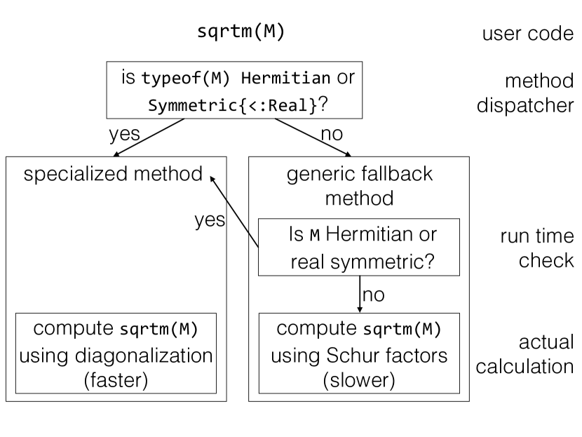
Figure 1: Dynamic dispatch and multimethods for the matrix square root function sqrtm, showing that the specialized algorithm can be run either from a static decision from the method dispatcher based on the input type, or a dynamic decision from a run-time check based on the value.

2.3 Resolving Dispatch Statically

This example illustrates a pattern characteristic of technical computing environments: dynamic dispatch on top of statically-typed performance kernels. However the difference here is that both components can be expressed in the same language, and with the same notation. [Talk about the static dispatch algorithm.]

[Incorporate Jeff’s example from his thesis.]

2.4 Polymorphic types in Julia

[This part of the story seems to not be front and center anymore. What should we do about it?]

Code specialization is only half of the story. The other half is extensibility — adding new data types and method definitions. Julia’s approach to extensibility is designed to take advantage of specialization, by allowing methods to be defined for combinations of structured types.

The method shown above demonstrates two kinds of polymorphism supported in Julia. First, the input A is annotated (::) with the type StridedMatrix, which is an abstract type, not a concrete type. A strided matrix is one that has a Fortran-compatible storage format, i.e. it is stored in a contiguous block of memory and whose dimensions can be described by a dope vector. The subtypes of StridedMatrix in the base library are Matrix (ordinary matrices), and subarray types defining views into strided matrices, whose referenced elements may not be fully contiguous in memory. Thus, this sqrtm method would be dispatched upon by both Matrix objects and subarrays, by virtue of both types being subtypes of StridedMatrix.

The second kind of polymorphism shown by the signature sqrtm{T<:Real}(A::Matrix{T}) is parametric polymorphism. This signature defines a family of related methods, one for each kind of Matrix containing a numeric type T that is a subtype (<:) of Real. This definition encompasses separate definitions for matrices of type Matrix{Int32} (matrices of 32-bit integers), Matrix{Float64} (matrices of 64-bit floating point real numbers), and even Matrix{Rational{BigInt}} (matrices of rational numbers where the numerators and denominators are arbitrary precision integers). Matrices containing other types, such as Matrix{Complex{Float64}}, would not dispatch on this family of methods.

The two kinds of polymorphism allow families of related methods to be defined concisely, which allow highly generic code to be written. Additionally, code for multiple algorithms can coexist within the same generic function, with the actual choice of which code to run being determined by method dispatch. Furthermore, the same performant kernel can be called even in situations where the user does not know that a particular input matrix is symmetric, or even that specialized algorithms for symmetric matrices exist.

3 Type system

Julia uses run-time type tags to describe and differentiate objects by their representation and behavior [Pierce, 2002, Section 11.10, p. 142]. We tend to use the term “type” instead of “tag”, as most programmers seem comfortable with this usage Tratt [2009]; Kell [2014].

Tags are useful for both users and compilers for deciding what to do to values, but incur overhead which increases the memory footprint of a data item. This overhead motivates most dynamically typed languages to simplify and minimize their tag systems.

Julia is unusual in allowing type tags with nested structure, forming nearly arbitrary symbolic expressions. This has two immediate benefits: first, it expands the criteria programmers have available for dispatching methods, and second, provides richer information to the compiler. Julia’s type tags are designed to serve as elements of a lattice, facilitating data flow analysis.

Julia types are first-class values, allowing programs to compute with them. In technical computing it is unusually common to perform a non-trivial computation to determine, for example, which data type to use for an operation. Julia allows this to be done using ordinary code.

3.1 Kinds of types

In addition to tags, Julia has three other kinds of types, which together form its full type lattice. There are abstract types, which form a nominal subtyping hierarchy. Abstract types may serve as declared supertypes of tag types or of other abstract types. Union types are used to form the least upper bound of any two types. Finally, existential types can be used to quantify over a type.

Tag types can have associated memory representations, corresponding to struct, primitive, and array types familiar to the C language family.

3.2 Subtyping

Julia requires abstract and tag types to have exactly one declared supertype, defaulting to Any (i.e. $\top$) if not explicitly declared. We conjecture that the subtype relation <: is well-defined and decidable, and that types are closed under meet ($\wedge$) and join ($\vee$).

3.3 Type parameters

Abstract and tag types can have one or more parameters. These types are superficially similar to parametric types in existing languages, but are actually intended simply for expressing information, rather than implementing the formal theory of parametric polymorphism.

The following example, from Julia’s standard library, describes a SubArray type that provides an indexed “view” into another array. Such array views enable different indexing semantics to be overlaid on an existing array. The SubArray type defines a Union of what kinds of indexes may be used, then uses this definition to define indexed views:

⬇

typealias RangeIndex Union(Int,Range{Int},

UnitRange{Int})

type SubArray{T, N, A<:AbstractArray,

I<:(RangeIndex...,)} <: AbstractArray{T,N}

# definition body omitted

end

SubArray has parameters T for an element type, N for the number of dimensions, A for the underlying array type, and I for the tuple of indexes that describe which part of the underlying array is viewed. (RangeIndex...,) denotes a tuple (essentially an immutable vector) of any number of RangeIndex objects. The final <: declares SubArray to be a subtype of AbstractArray.

Julia’s type system tries to hide type kinds from the user. The identifier SubArray by itself does not refer to a type constructor that must be instantiated. Rather, it is a type that serves as the supertype of all the SubArray types. This allows convenient shorthand for method signatures that are agnostic about type parameters. It also makes it possible to add more type parameters in the future, without being forced to update all code that uses that type. This is achieved by making SubArray an existential type with bounded type variables.

When implementing SubArray and client code using it, it is useful to be able to dispatch on all of these parameters. For example, when I matches (UnitRange, RangeIndex...) then the SubArray is contiguous in the leading dimension, and more efficient algorithms can generally be used. Or, linear algebra code might want to restrict the number of dimensions N to 1 or 2.

3.3.1 Variance

The subtyping rules for parametric types require reasoning about variance, i.e. the relation between subtype relations of the parametric types and subtype relations of the parameters. The conventional wisdom is that type safety allows covariance if components are read but not written, and contravariance if they are written but not read Castagna [1995]. As type parameters can represent the types of mutable fields, the only safe choice is invariance. Thus Julia’s parametric types are invariant.

Parametric invariance has some subtle consequences for Julia’s type system. First, parametric types introduce many short, finite length chains into the type lattice. Consider the simple type system of Figure 2a, with two leaf (instantiable types) types 1 and 2 representing singleton values 1 and 2 of the natural numbers Nat. A user can augment the lattice with a new parametric type S{T}. If there is no restriction whatsoever on the type parameter T, then there are 5 different parametric types of the form S{T}. Furthermore, each S{T} has supertype S by construction, and by invariance of T there are no values of the type parameters T and U such that S{T} is a subtype of S{U}. Additionally, none of the types S{T} is a subtype or supertype of any of 1, 2 or Nat. Thus each S{T} appears in exactly one finite poset $\bot$ <: S{T} <: S <: $\top$, and the new type lattice has the structure shown in Figure 2b. Note that S{$\top$} is a concrete type with type parameter $\top$ (Any), while S{T} is a synonym for the abstract type S where T is a type variable with lower bound $\bot$ and upper bound $\top$.

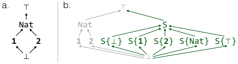
Figure 2: a. A simple lattice with bottom type $\bot$, top type $\top$, singleton types 1 and 2, and their supertype Nat. b. The same lattice extended with a parametric type S{T} with no restriction on the type parameter T, showing that for each T, invariance requires that the corresponding type S{T} be a leaf type (i.e. instantiable), even if T itself is not a leaf type.

3.4 Function types

Julia is higher-order; functions can be passed to and returned from other functions. However, the language currently does not have function (arrow) types. The reason for this is that a Julia function need not have a useful canonical return type. We could consider every function to have return type Any, but this is not terribly revealing. Return types based on Julia’s type inference would not be predictable, as inference is heuristic and best-effort. Future compiler improvements can make inferred types more specific, and this should not effect program behavior (only performance).

Julia does support nominal function types — a data type may implement the call generic function, allowing it to be used anywhere a function can be used.

3.5 Type conversion

While Julia code can be written without explicitly reasoning about types, the ability to do so is sometimes necessary for understanding code performance issues. Julia provides the convert(T, x) function which converts a value x to its corresponding representation in the type T. This is a generic function like any other, but since T is typically a compile-time constant, convert this can serve as a mechanism for limiting polymorphism in code where performance considerations are important.

The idea of converting a value of type A to type B does not naturally belong to one type or the other, which favors multiple dispatch over classes. Conversion also benefits from open extension: mathematical objects often have embeddings in multiple domains, not all of which might be known or desired by the original author of some code. For example, numbers can be embedded in matrices with diagonal matrices, but not all users are likely to find this correspondence helpful.

4 Generic functions and multimethods

Mathematical thought is naturally polymorphic. Multimethods are a natural mechanism for capturing such polymorphism Bezanson et al. [2014b]; Chen and Edelman [2014]. Consider an operation as fundamental as multiplication: an expression like a*b can mean a matrix-matrix product, a matrix-vector product, or a scalar-vector product, to name just a few possibilities. A generic function system supporting multimethods allows for the * function to be polymorphic, expressing a common metaphor for different kinds of multiplication which can be disambiguated by the types of a and b. In contrast, languages supporting only classes cannot capture the full extent of polymorphism in * in method dispatch: as classes inherently support only single dispatch on the first argument, each method * defined for each class a must contain different code blocks for each possible type of b, thus in practice requiring multiple dispatch to be emulated using virtual methods and visitor patterns Gamma et al. [1995]. Furthermore, implementing binary methods can require knowing the internal representation of both objects a and b, especially for performance reasons Bruce et al. [1995]. Such knowledge fundamentally corrupts the abstraction of class-based encapsulation, as the methods associated with a must know implementation details of all possible objects b that a may interact with. In contrast, there is no abstraction leak associated with allowing a generic function * knowledge about the internal representations of the types it works on.

Multiplication represented by * can be extended, for example, to multiplication between quaternions, or even to $N$-ary matrix-matrix products, where associativity allows matrix-matrix products to be regrouped so as to minimize the total memory footprint and operation count Hu and Shing [1984].

The extensibility of Julia’s generic functions and types allow users to define new behaviors that intermix new types and new functions. The price we pay for such flexibility, of course, is that dynamic function dispatch incurs greater overhead: unlike in a single dispatch language, multiple lookups in method tables may be necessary to determine which method is most appropriate Bruce et al. [1995]. Type inference is useful for minimizing or even eliminating the overhead associated with multiple dispatch.

Many of the use cases for multiple dispatch could potentially be addressed by operator overloading as in C++. However C++ forces programmers to choose which operations will use dynamic dispatch (via virtual methods), which will use templates, and which will use function overloading. We conjecture that this choice can be an unwelcome productivity drain. For example, the syntactic difference between function calls and method calls could require code to be rewritten when requirements change, or could lead to APIs that are not consistent about when method calls are used.

5 Type inference

It is well known that type inference can be used to move tag manipulations and method lookup to compile time, thus eliminating most overhead from the execution of dynamically-typed code Kaplan and Ullman [1977, 1980]. Data flow type inference Nielson et al. [2005]; Khedker et al. [2009] is especially useful in this context, as its flow-sensitivity yields good type information even if the type of a program variable is different at different points in the code. Data flow analysis, particularly in the forward direction, captures the human intuition of how programs work: values start at the top and move through the program step by step. Another advantage of this approach is that it is not speculative: it yields correct deductions about types that, in the best case, allow overhead to be removed entirely. This property is important to technical users, who need languages that can match the performance of C and Fortran.

Unfortunately, data flow type inference can be defeated by dynamic language programs that are too “type complex”. If the library functions used might return too many different types, or there are too many paths through user code, the resulting type information might not be useful.

Julia was designed to help mitigate this problem. By encouraging code to be written in small pieces labeled with type information (for dispatch), it is easier for the compiler to rule out execution paths that do not actually occur.

Type inference in Julia occurs after code is parsed, macro-expanded, and lowered into a static single assignment (SSA) intermediate representation (IR) Alpern et al. [1988]; Rosen et al. [1988] that facilitates data flow analysis Cousot and Cousot [1977, 2000]; Nielson et al. [2005] and is relatively straightforward to map onto LLVM IR Lattner and Adve [2004]. Julia uses Mohnen’s algorithm for abstract interpretation Cousot and Cousot [1992a] which works directly on the SSA IR Mohnen [2002]. The abstract semantics are described internally using transfer functions (a.k.a. t-functions or flow functions), which approximate program semantics by inferring possible output types based on the types of the inputs.

In practice, the expressiveness of Julia’s late binding semantics, combined with the presence of potentially infinite types such as varargs tuples (T...), complicate type inference. Therefore practical type inference necessitates widening heuristics, which reduce computational costs and guarantee termination in the presence of recursive types Cousot and Cousot [1992b]. Examples of such heuristics include widening (pessimizing) type unions and tuple types which exceed a certain length, and limiting the maximal depths of types and tuples analyzed.

Julia provides language features to help users inspect the results of type inference and specify additional type information where necessary to sharpen the types of variables.

1. The base library provides introspection functions like code_typed, which allow users to inspect generated type annotations and avoid second-guessing the compiler’s intentions.

2. Variables can also be given explicit type annotations; changing x = 0 to x::Float64 = 0 declares x to be of type Float64 within the current scope, and all assignments x = _ implicitly call the type conversion function convert(Float64, _).

3. Expressions can be given type assertions; changing x += y to x += y :: Int asserts that y must be of type Int or otherwise raise a run-time error.

External packages like TypeCheck.jl and Lint.jl provide further static analyses which are useful for detecting type-related issues.

6 Applications in technical computing

In this section, we describe how the type system, generic functions and type inference interact in Julia code for scientific computations in base library code as well as registered packages.

6.1 Type promotion

The type system and generic function system allow for type promotion rules to be specified in the base library rather than be hard-coded into a given implementation Bezanson [2012]. For example, simple arithmetic functions on general numeric types in Julia’s base library contain methods of the form:

⬇

+(x::Number, y::Number) = +(promote(x,y)...)

*(x::Number, y::Number) = *(promote(x,y)...)

-(x::Number, y::Number) = -(promote(x,y)...)

/(x::Number, y::Number) = /(promote(x,y)...)

^(x::Number, y::Number) = ^(promote(x,y)...)

For example, an operation like 2 * 3.4 is evaluated under the hood as follows:

⬇

*(2, 3.4) = *(promote(2, 3.4)...)

= *(convert(promote_type(Int,Float64),2),

convert(promote_type(Int,Float64),3.4))

= *(convert(Float64,2), convert(Float64,3.4))

= *(2.0, 3.4)

= 6.8

where promote(x, y) promotes the values x and y to numerically equivalent values of a common supertype, and promote_type(S,T) computes a common supertype of S and T. The latter calls a custom promotion rule, if defined, and defaults otherwise to the join S$\vee$T.

Type promotion allows for different functions and methods to share a common and consistent logic for polymorphism. The implementation of type promotion leverages the type system to allow for greater code reuse across different methods and functions. Furthermore, it is a part of the Julia language which can be built entirely from other language constructs.

6.2 Numerical linear algebra library

Designing a general-purpose linear algebra library involves several different layers of complexity, and has been described as implementing the following meta-program Demmel et al. [2007]:

(1) for all linear algebra problems
    (linear systems, eigenproblems, ...)
(2)  for all matrix types
     (general, symmetric, banded, ...)
(3)   for all data types (real, complex,
      single, double, higher precision)
(4)    for all machine architectures and
       communication topologies
(5)     for all programming interfaces
(6)      provide the best algorithm(s) available
         in terms of performance and accuracy
         (‘‘algorithms’’ is plural because
         sometimes no single one is always best)

The six-tiered hierarchy neatly delineates how the basic collection of linear algebra problems (1) have to be specialized by data representation (2–3) and machine details (4), which are then used to decide which specific algorithms (5–6) to use.

Many systems provide optimized implementations of standard libraries for numerical linear algebra like BLAS (Basic Linear Algebra Subprograms) and LAPACK (Linear Algebra PACKage) Anderson et al. [1999]. Computational routines can be customized for individual microarchitectures and can reach a large fraction of theoretical peak FLOPS. However, these libraries inherit archaic Fortran 77 interfaces and hence tend to restrict routine names to six letters or shorter. When combined with the lack of polymorphism in Fortran, the names are terse and cryptic to nonexperts: a typical routine like DSTEV solves the eigenvalue problem (EV) for symmetric tridiagonal matrices (ST) with double precision floating point entries (D), and furthermore takes eight positional arguments specifying the inputs, outputs, computation mode, and scratch variables. The lack of polymorphism results in redundancy due to lack of code reuse, which hinders the implementation of new algorithms (which have to be reimplemented for each level of floating-point precision) and new routines for such as mixed-precision and quad precision routines (which must implement all the existing algorithms).

The code redundancy problem is largely ameliorated with the combination of type polymorphism and dynamic multiple dispatch. The six-tiered hierarchy above maps naturally onto different language constructs in Julia as follows:

Tier	Description	Language construct
1	linear algebra problems	generic function
2	matrix types	parametric types
3	data types	type parameter
4	machine architectures	method body
5	programming interfaces	generic function
6	(poly)algorithms	method body

The generic function system allows for fast specializations and generic fall-backs to coexist, thus allowing for speed when possible and flexibility otherwise. For example, Julia provides generic fall-back routines to do matrix computations over arbitrary fields of element types, providing the ability to compute on numeric types which are not mappable to hardware floating point types. This can be useful to perform matrix computations in exact rational arithmetic or software-emulated higher precision floating point arithmetic to verify the implementations of algorithms or to detect the possibility of numerical instability associated with roundoff errors. These general purpose routines coexist with BLAS and LAPACK wrappers, thus allowing dispatch onto performant code when available, and general code otherwise. User code can be written that will work regardless of element type (Tier 3), and can be tuned for performance later.

6.3 Generic linear algebra

Code for technical computing often sacrifices abstraction for performance, and is less expressive as a result. In contrast, mathematical ideas are inherently polymorphic and amenable to abstraction. Consider a simple example like multiplication, represented in Julia by the * operator. * is a generic function in Julia, and has specialized methods for many different multiplications, such as scalar–scalar products, scalar–vector products, and matrix–vector products. Expressing all these operations using the same generic function captures the common metaphor of multiplication.

6.4 Bilinear forms

Julia allows user code to extend the * operator, which can be useful for more specialized products. One such example is bilinear forms, which are vector–matrix–vector products of the form

$$\gamma=v^{\prime}Mw=\sum_{ij}v_{i}M_{ij}w_{j}$$ (1)

This bilinear form can be expressed in Julia code as

⬇

function (*){T}(v::AbstractVector{T},

M::AbstractMatrix{T},

w::AbstractVector{T})

if !(size(M,1) == length(v) &&

size(M,2) == length(w))

throw(BoundsError())

end

$\gamma$ = zero(T)

for i = 1:size(M,1), j = 1:size(M,2)

$\gamma$ += v[i] * M[i,j] * w[j]

end

return $\gamma$

end

The newly defined method can be called in an expression like v * M * w, which is parsed and desugared into an ordinary function call *(v, M, w). This method takes advantage of the result being a scalar to avoid allocating intermediate vector quantities, which would be necessary if the products were evaluated pairwise like in $v^{\prime}(Mw)$ and $(v^{\prime}M)w$. Avoiding memory allocation reduces the number of heap-allocated objects and produces less garbage, both of which are important for performance considerations.

The method signature above demonstrates two kinds of polymorphism in Julia. First, both AbstractVector and AbstractMatrix are abstract types, which are declared supertypes of concrete types. Examples of subtypes of AbstractMatrix include Matrix (dense two-dimensional arrays) and SparseMatrixCSC (sparse matrices stored in so-called compressed sparse column format). Thus the method above is defined equally for arrays of the appropriate ranks, be they dense, sparse, or even distributed. Second, T defines a type parameter that is common to v, M and w. In this instance, T describes the type of element stored in the AbstractVector or AbstractMatrix, and the {T}(...{T}...{T}) syntax defines a family of methods where T is the same for all three arguments. The type parameter T can also used in the function body; here, it is used to initialize a zero value of the appropriate type for $\gamma$.

The initialization statement $\gamma$ = zero(T) requests a zero element of the appropriate type. In Julia this is important because using a zero value of a different type can cause a different method to be called. If T is any concrete type, e.g. Float64 (64-bit floating point real numbers), then Julia’s just-in-time compiler can analyze the code statically to remove type checks. For example, in the method with signature *{Float64}(v::AbstractVector{Float64}, M::AbstractMatrix{Float64}, w::AbstractVector{Float64}), the indexing operations on $v$, $M$ and $w$ always return Float64 scalars. Furthermore, forward data flow analysis allows the type of $\gamma$ to be inferred as Float64 also, since floating point numbers are closed under addition and multiplication. Hence, type checks and method dispatch for functions like + and * within the function body can be resolved statically and eliminated from run time code, allowing fast code to be generated.

Were we to replace the initialization with the similar-looking $\gamma$ = 0, we would have instead a type instability when T = Float64. Because $\gamma$ is initialized to an Int (native machine integer) and it is incremented zero or more times by a Float64 in the for loop, the type of the variable can change at run time. In fact, the result type will depend on the size of the input array $M$, which is only known at run time. Julia allows this behavior, and our compiler infers the type of $\gamma$ to be Union(Int,Float64), which is the least upper bound on the actual type of $\gamma$ at run time. As a result, not all type checks and method dispatches can be hoisted out of the loop body, resulting in slower execution.

6.5 Matrix equivalences

Matrix equivalences are another example of specialized product that users may want. Two $n\times n$ matrices $A$ and $B$ are considered equivalent if there exist invertible matrices $V$ and $W$ such that $B=V*A*W^{\prime}$. Oftentimes, equivalence relations are considered between a given matrix $B$ and another matrix $A$ with special structure, and the transformation $(W^{\prime})^{-1}\cdot V^{-1}$ can be thought of as changing the bases of the rows and columns of $B$ to uncover the special structure buried within as $A$. Matrices with special structure are ubiquitous in numerical linear algebra. One example is rank-$k$ matrices, which can be written in the outer product form $A=XY^{\prime}$ where $X$ and $Y$ each have $k$ columns. Rank-$k$ matrices may be reified as dense two-dimensional arrays, but the matrix–matrix–matrix product $V*A*W^{\prime}$ would take $O(n^{3})$ time to compute. Instead, when $k\ll n$, the product be computed more efficiently in $O(kn^{2})$ time, since

$$VAW^{\prime}=V(XY^{\prime})W^{\prime}=(VX)(WY)^{\prime}$$ (2)

and the result is again a rank-$k$ matrix. Furthermore, we can avoid constructing $W^{\prime}$, the transpose of $W$, explicitly. Therefore in some cases, it is sensible to store $A$ as the two matrices $X$ and $Y$ separately, rather than as a reified 2D array.

Julia allows users to encapsulate $X$ and $Y$ within a specialized type:

⬇

type OuterProduct{T}

X :: Matrix{T}

Y :: Matrix{T}

end

Defining the new OuterProduct type has the advantage of grouping together objects that belong together, but also enables dispatch based on the new type itself. We can now write a new method for *:

⬇

*(V, M::OuterProduct, W) = OuterProduct(V*M.X, W*M.Y)

This method definition uses a convenient one-line syntax for short definitions instead of the function ... end block. This method also does not annotate V or W with types, and so they are considered to be of the top type $\top$ (Any in Julia). This method may be called with any $V$ and $W$ which support premultiplication: so long as V*M.X and W*M.Y are defined and produce matrices of the same type, then the code will run without errors (“duck typing”). This flexibility is convenient since $V$ and $W$ can now be scalars or matrixlike objects which themselves have special structures, or even more generally could represent linear maps that are not stored explicitly, but rather defined implicitly through their actions when multiplying a Matrix on the left.

The preceding method shows that Julia does not require all method arguments to have explicit type annotations. Instead, dynamic multiple dispatch allows the argument types to be determined from the arguments at run time. Julia’s just-in-time compiler will be invoked when the method is first called, so that static analyses can be performed.

We can now proceed to define a new type and method

⬇

type RowPermutation

p::Vector{Int}

end

*($\Pi$::RowPermutation, M::Matrix) = M[$\Pi$.p, :]

whose action can be thought of as multiplying by a permutation matrix on the left, resulting in a version of $M$ with the rows permuted. Now, the following user code

⬇

n = 10

k = 2

X = randn(n, k) #Random matrix of Float64s

M = OuterProduct(X, X)

p = randperm(n) #Random permutation of length n

$\Pi$ = RowPermutation(p)

M2 = $\Pi$ * M * $\Pi$

will dispatch on the appropriate methods of * to produce the same result M2 as

⬇

M2 = OuterProduct(M.X[p, :], M.Y[p, :])

In other words, the specialized method *(::RowPermutation, ::OuterProduct{Float64}, ::RowPermutation) is compiled only when it is first invoked in the creation of M2, since it follows from composing the method defined with signature *(::Any, ::OuterProduct, ::Any) with the argument tuple of type (RowPermutation, OuterProduct{Float64}, RowPermutation).

6.6 Matrix factorization types

Julia’s base linear algebra library also provides extensive support for matrix factorizations, which are indispensable for reasoning about the interdependencies between matrices with special properties and the numerical algorithms that they enable Golub and Van Loan [2013]. Many algorithms for numerical linear algebra involve interconversions between general matrices and similar matrices with special matrix symmetries. For many purposes, it is convenient to reason about the resulting special matrix, together with the matrix performing the transformation, as a single mathematical object rather than two separate matrices. Such an object represents a matrix factorization, and is essentially a different data structure that can represent the same content as a matrix represented as an ordinary two-dimensional array.

The exact matrix factorization object relevant for a given linear algebra problem depends on the symmetries of the starting matrix and also the underlying field of matrix elements (i.e. whether the matrix contains real numbers, complex numbers, or something else). In some use cases, these properties may be known by the user as part of the problem specification, and in other cases they may be unknown. Some properties, like whether a matrix is triangular, can be deduced by inspecting the matrix elements for $O(N^{2})$ cost. Others, like whether a matrix is positive definite, require an $O(N^{3})$ computation in the general case, and is most efficiently determined by attempting to compute the Cholesky factorization.

The resulting algorithm for determining a useful matrix factorization has to capture the interplay between allowing the user to specify additional matrix properties and attempting to automatically detect useful properties when the additional cost of doing so is not prohibitive. The general case is implemented in Julia’s base library by the factorize function, and typifies the complexity associated with numerical codes:

⬇

function factorize{T}(A::Matrix{T})

m, n = size(A)

if m != n

# A is rectangular

# Can the result of a QR factorization be represented

# using a floating point type supported by BLAS?

BlasFloat = Union(Float32,Float64,Complex64,Complex128)

rt = zero(T) / sqrt(zero(T) + zero(T))

can_use_BlasFloat = isa(rt, BlasFloat)

# Factorize into pivoted QR form where possible,

# otherwise compute (unpivoted) QR form

return qrfact(A, pivot=can_use_BlasFloat)

end

# A is square

# The factorization of a 1x1 matrix is just itself

m == 1 && return A[1]

utri = istriu(A) # upper triangular?

utri1 = ishessenbergu(A) # upper Hessenberg?

sym = issym(A)

herm = ishermitian(A)

ltri = istril(A) # lower triangular?

ltri1 = ishessenbergl(A) # lower Hessenberg?

if ltri && utri

return Diagonal(A)

elseif ltri && utri1

return Bidiagonal(diag(A), diag(A, -1), false)

elseif ltri

return Triangular(A, :L)

elseif ltri1 && utri

return Bidiagonal(diag(A), diag(A, 1), true)

elseif ltri1 && utri1

if (herm && (T <: Complex)) || sym

M = SymTridiagonal(diag(A), diag(A, -1))

# _may_ be factorizable into

# LDL’ Cholesky form

try

return ldltfact!(M)

end

end

# Factorize into tridiagonal LU form

M = Tridiagonal(diag(A,-1), diag(A), diag(A,1))

return lufact!(M)

elseif utri

return Triangular(A, :U)

elseif herm

# try to factorizable into Cholesky form

try

return cholfact(A)

end

# else use general Hermitian factorization

return factorize(Hermitian(A))

elseif sym

# Use general Symmetric factorization

return factorize(Symmetric(A))

else

# A is square but has no other symmetries

# Factorize into LU form

return lufact(A)

end

end

# Factorize a Hermitian or Symmetric matrix into

# Bunch-Kaufman form as computed by bkfact

typealias HermOrSym Union(Hermitian,Symmetric)

factorize(A::HermOrSym) =

bkfact(A.data, symbol(A.uplo), issym(A))

The factorize function contains a few interesting features designed to capture the highly dynamic nature of this computation:

1. The beginning checks for the “easy” properties, i.e. those that can be computed cheaply at run-time by inspecting the matrix elements. The presence of one or more of these properties allow the input matrix A to be classified into several special cases.

2. For many of these special cases (like Diagonal), A is explicitly converted to a special matrix type which allows dispatch on efficient specializations of linear algebraic operations that users may choose to perform later, such as matrix multiplication.

3. For other special cases (like Tridiagonal), it is useful to attempt a run-time check for the “hard” properties, like positive definiteness, which require nontrivial computation. Computing the Cholesky factorization serves both as an efficient run-time check to detect positive definiteness, whose failure indicates lack thereof, and whose success yields a useful Cholesky matrix factorization object which is useful for further computations such as solving linear equations or computing singular value decompositions (SVDs).

4. The Symmetric and Hermitian cases use control flow enabled by dynamic multimethods, as it is common for users to know whether the matrices they are working with have these properties. Using multimethods allows users to elide all the run-time checks in the generic method, skipping directly to the appropriate specialized method.

5. The base case contains a nontrivial runtime check to determine if the element type of A{T} can be represented as a hardware-representable real or complex floating point number. The canuseBlasFloat variable computes the type resulting from computations of the form $x/\sqrt{x+x}$, and checks that it is a subtype of BlasFloat. The reason for this check is that there are two variants of the QR factorization: one pivoted, the other not.

In theory, it is possible to combine these structured matrix types under a tagged union, e.g. in an ML-family language. However this would be less convenient. The problem is that in most contexts, users are happy to have these objects separated by the type system, but certain functions like factorize wish to combine them. It should be possible to pass the result of such a function directly to an existing routine that expects a particular matrix structure, without needing to interpose case analysis to handle a tagged union.

It is also instructive to look more carefully at the methods for bkfact, which is but one of the several factorizations computed in factorize:

⬇

# Compute Bunch-Kaufman factorization,

bkfact{T<:BlasFloat}(A::StridedMatrix{T},

uplo::Symbol=:U,

sym::Bool=issym(A)) =

bkfact!(copy(A),uplo,sym)

function bkfact{T}(A::StridedMatrix{T},

uplo::Symbol=:U,

sym::Bool=issym(A))

Typ = promote_type(Float32,

typeof(sqrt(one(T))))

bkfact!(Matrix{Typ}(A),uplo,symmetric)

end

# Compute Bunch-Kaufman factorization in-place

# call LAPACK SSYTRF/DSYTRF where possible

function bkfact!{T<:BlasReal}(A::StridedMatrix{T},

uplo::Symbol=:U,

sym::Bool=issym(A))

if sym

error("The Bunch-Kaufman decomposition ",

"is only valid for symmetric matrices")

end

LD, ipiv = LAPACK.sytrf!(char_uplo(uplo),A)

BunchKaufman(LD,ipiv,char_uplo(uplo),symmetric)

end

function bkfact!{T<:BlasComplex}(A::StridedMatrix{T},

uplo::Symbol=:U,

sym::Bool=issym(A))

if sym

LD,ipiv = LAPACK.sytrf!(char_uplo(uplo),A)

else

LD,ipiv = LAPACK.hetrf!(char_uplo(uplo),A)

end

BunchKaufman(LD,ipiv,char_uplo(uplo),sym)

end

The Bunch-Kaufman routines are implemented in two functions: bkfact, which allocates new memory for the answer, and bkfact!, which mutates the matrix in place to save memory. Reasoning about memory use is critical in numerical linear algebra applications as the matrices may be large. Reusing allocated memory for matrices also avoids unnecessary copies of data to be made, potentially minimizing memory accesses and reducing the need to trigger garbage collection. The base library thus provides the latter for users who need to reason about memory usage, and the former for users who do not.

The syntax {T<:BlasReal} in a method definition implicitly wraps the signature in a UnionAll type. As a result, the method matches all matrices whose elements are of a type supported by BLAS.

7 Case study: completely pivoted LU

Linear algebra is ubiquitous in technical computing applications. At the same time, the implementation of linear algebra libraries is generally considered a difficult problem best left to the experts. A popular reference book for numerical methods famously wrote, for example, that “the solution of eigensystems… is one of the few subjects covered in this book for which we do not recommend that you avoid canned routines” [Press et al., , Section 11.0, p. 461]. While much effort has been invested in making numerical linear algebra libraries fast Anderson et al. [1999]; Gunnels et al. [2001]; Zhang et al. [2012]; Van Zee and Van de Geijn [2013], one nevertheless will occasionally need an algorithm that is not implemented in a standard linear algebra library.

One such nonstandard algorithm is the completely pivoted LU factorization. This algorithm is not implemented in standard linear algebra libraries in LAPACK Anderson et al. [1999], as the conventional wisdom is the gains in numerical stability in complete pivoting is not generally worth the extra effort over other variants such as partial pivoting Golub and Van Loan [2013]. Nevertheless, users may want complete pivoting for comparison with other algorithms for a particular use case.

In this section, we compare implementations and performance of this algorithm in Julia with other high level languages that are commonly used for technical computing: MATLAB, Octave, Python/NumPy, and R.

7.1 Naïve textbook implementation

Algorithm 1 presents the textbook description of the LU factorization with complete pivoting [Golub and Van Loan, 2013, Algorithm 3.4.3 (Outer Product LU with Complete Pivoting), p. 132], and below it a direct translation into a naïve Julia implementation. This algorithm is presented in MATLAB-like pseudocode, and contains a mixture of scalar for loops and MATLAB-style vectorized indexing operations that describe various subarrays of the input matrix $A$. Additionally, there is a description for the subproblem of finding the next pivot at the start of the loop. Furthermore, the pseudocode uses the $\leftrightarrow$ operation, denoting swaps of various rows and columns of $A$. To translate the pivot finding subproblem into Julia, we used the built-in indmax function to find the linear index of the value of the subarray A[k:n, k:n] which has the largest magnitude, then used the ind2sub function to convert the linear index to a tuple index. The $\leftrightarrow$ operator was implemented using vectorized indexing operations, as is standard practice in high level languages like MATLAB.

Algorithm 1 Top: Textbook pseudocode describing the $LU$ factorization with complete pivoting [Golub and Van Loan, 2013, Algorithm 3.4.3 (Outer Product LU with Complete Pivoting), p. 132]. The matrix $A$ is overwritten in-place with the $LU$ factors, with $rowpiv$ and $colpiv$ containing the row and column pivots respectively. Bottom: An implementation of $LU$ factorization with complete pivoting in Julia, which returns the result as a tuple. The ! at the end of the function name is convention for a function with side effects (in this case, mutating $A$). Unicode characters such as Greek letters and the $\neq$ operator are allowed in Julia code, allowing for close notational correspondence with the textbook description of the algorithm.

for $k=1:n-1$ do Determine $\mu,\lambda$ where $k\leq\mu\leq n$, $k\leq\lambda\leq n$, so $\quad\left|A(\mu,\lambda)\right|=\max\{\left|A(i,j)\right|:i=k:n,j=k:n\}$ $rowpiv(k)=\mu$ $A(k,1:n)\leftrightarrow A(\mu,1:n)$ $colpiv(k)=\lambda$ $A(1:n,k)\leftrightarrow A(1:n,\lambda)$

     if $A(k,k)\neq 0$ then $\rho=k+1:n$ $A(\rho,k)=A(\rho,k)/A(k,k)$ $A(\rho,\rho)=A(\rho,\rho)-A(\rho,k)A(k,\rho)$

     end if

end for

⬇

function lucompletepiv!(A)

n=size(A, 1)

rowpiv=zeros(Int, n-1)

colpiv=zeros(Int, n-1)

for k=1:n-1

Asub = abs(A[k:n, k:n]) #Search for next pivot

$\mu$, $\lambda$ = ind2sub(size(Asub), indmax(Asub))

$\mu$ += k-1; $\lambda$ += k-1

rowpiv[k] = $\mu$

A[[k, $\mu$], 1:n] = A[[$\mu$, k], 1:n]

colpiv[k] = $\lambda$

A[1:n, [k, $\lambda$]] = A[1:n, [$\lambda$, k]]

if A[k,k] $\neq$ 0

$\rho$ = k+1:n

A[$\rho$, k] = A[$\rho$, k]/A[k, k]

A[$\rho$, $\rho$] = A[$\rho$, $\rho$] - A[$\rho$, k] * A[k, $\rho$]

end

end

return (A, rowpiv, colpiv)

end

For comparison purposes, we also wrote naïve implementations in other high level dynamics languages which are popular for technical computing. Here, we considered MATLAB The MathWorks Inc. [2014], Octave Eaton et al. [2009], Python van Rossum [1995]/NumPy Van Der Walt et al. [2011], and R R Development Core Team [2008] (whose codes are available in the Appendix). The codes were executed on a late 2013 MacBook Pro running OS X Yosemite 10.10.2, with Julia 0.4-dev+3970, MATLAB R2014b, Octave 3.8.1, Python 3.4.3 with NumPy 1.9.2 from the Anaconda 2.1.0 distribution, and R 3.1.3. Where possible, we also tried to run variants with and without JIT compilation. In MATLAB, the JIT compiler is on by default, but can be turned off with the command feature accel off. Octave’s JIT compiler is experimental and off by default, but can be enable with a command line switch. R provides a JIT compiler in the compiler library package. We do not have JIT-compiled results for Python, as at this time of writing, neither PyPy 2.5.0 Bolz et al. [2009] nor Numba 0.17.0 was able to compile the code. The results are summarized in Figure 3, which shows the near-perfect $O(n^{3})$ scaling of the algorithm in each implementation, as well as in Figure 4, which shows the execution times across the different languages for a $1000\times 1000$ matrix of Float64s with randomly sampled standard Gaussians.

The results show that the naïve Julia implementation performs favorably with the implementations in Matlab and Octave, all of which are significantly faster than R’s implementation. Python’s implementation is somewhat faster, owing to the rank-1 update step (of A[$\rho$, $\rho$]) being done in place. Turning on or off the JIT did not significantly change the execution times for Matlab, Octave and R.

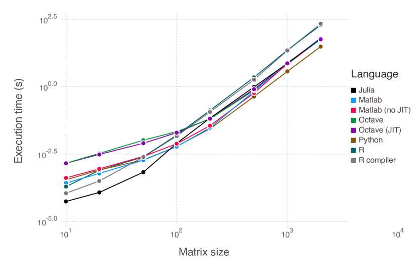
Figure 3: Scaling behavior of naïve implementations of the completely pivoted $LU$ algorithm on $N\times N$ random matrices in Julia, MATLAB, Octave, Python/NumPy, and R. By default, MATLAB’s JIT compiler is on, whereas Octave’s and R’s are off. Julia code is listed in Algorithm 1.

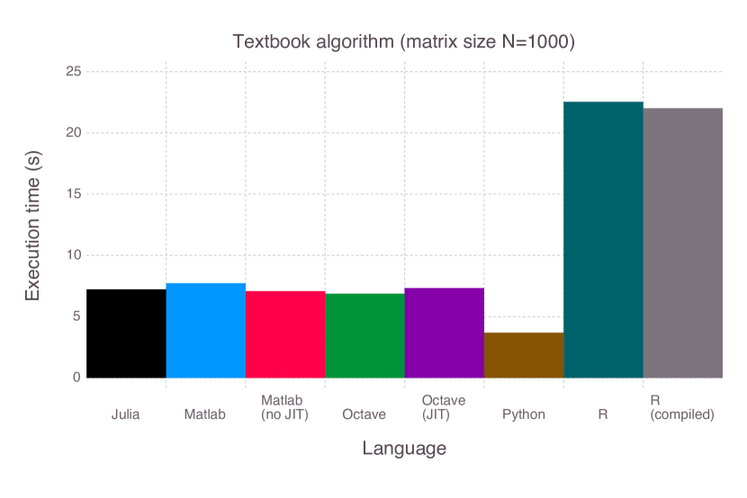
Figure 4: Execution times of naïve implementations of the completely pivoted $LU$ algorithm on a $1000\times 1000$ random matrix in Julia, MATLAB, Octave, Python/NumPy, and R. See Figure 3 for further details.

7.2 LU decomposition on arbitrary numeric types

One major advantage to writing the $LU$ factorization code in pure Julia is that lucompletepiv! can run on any Matrix{T}. So long as the underlying element type T is closed under the basic arithmetic operations +, -, *, /, abs, and max, the algorithm will run just as it did on Float64 numbers. For example, one could compute the completely pivoted $LU$ factorization on matrices of fixed point numbers (provided by the FixedPointNumbers.jl package), or matrices of rational numbers (built in Rational types).

⬇

#Initialize 1000x1000 matrix of 32-bit fixed point 1s

#with 14 fractional bits

using FixedPointNumbers

B = ones(Fixed32{14}, 1000, 1000)

lucompletepiv!(B)

#Initialize 1000x1000 matrix of unit rational numbers

#with 64-bit integer numerators and denominators

C = ones(Rational{Int64}, 1000, 1000)

lucompletepiv!(C)

Other interesting examples include the dual and hyperdual numbers provided by the DualNumbers.jl and HyperDualNumbers.jl packages respectively. Both types of numbers are used for forward mode automatic differentiation, and can be used with lucompletepiv! to take derivatives of the $LU$ factorization itself. Computations over such arbitrary numeric types would be difficult, if not impossible, in the other languages, without reimplementing the basic algorithm lucompletepiv! over and over again.

While of course it is possible to build in more numeric types to the base library of any programming language, the approach shown here is more general by virtue of being extensible by users. Other such numberlike quantities include colors (in Color.jl), unitful quantities (in SIUnits.jl), interval arithmetic (in ValidatedNumerics.jl), finite fields, dates and times (in Base.Dates), quaternions and octonions (in Quaternions.jl, extended precision floating point (in DoubleDouble.jl), DNA nucleotides (in BioSeq.jl), and many more.

7.3 Improving the performance of a naïve implementation

One of the reasons why high level languages are slow is that it allows the programmer to express algorithms in terms of array operations. These languages have a limited ability to optimize array expressions and consequently many temporary arrays are allocated during execution of a program.

In languages such as Fortran an C, similar algorithms are usually written without allocating temporary arrays. Some workspace might be required by the algorithm, but memory is then typically allocated once. This makes it possible to compile the code into efficient machine code that is typically much faster than what is possible for higher level array oriented languages.

In Julia, it is possible to express algorithms in terms of array operations, but it is also possible to avoid array allocations and thereby have the compiler optimizing the code to efficient machine code. Hence, a first step in optimizing Julia code is to find the lines during a loop that allocates temporary arrays.

The first line in the loop body makes two unnecessary array copies. The lines that flip columns and rows also allocate temporary arrays which can be avoided and allocations are also made for the scaling and rank one update in the last two lines of the if statement. By writing small auxiliary functions and expanding the scaling and rank one update as loops, it is possible to reduce the number of temporary allocations significantly.

For a square matrix of size 1000, a profiling of the naïve implementation reveals that it allocates more than 12 GB of memory and runs in 4.15 seconds. With the changes mentioned in last paragraph the memory allocation is only 7 MB and the running time reduces to 0.75 seconds. Typically, the avoidance of array allocation amounts to the largest share of speedup when optimizing Julia code, but it is possible to achieve a further speed improvement by annotating the code with two macros that turn off bounds checking on array indexing and allows the compiler to use SIMD registers when possible. This final optimization reduces the running time to 0.4 seconds.

In many cases it is not desired to write out array operations as loops, but it is convenient that this optimization is possible without reimplementing parts of or whole algorithms in C or Fortran first and then compile, link, and call these from the high level language. In Julia, the programmer can optimize incrementally and immediately see eventual speed improvements within a single language.

8 Related Work

There has been a rich history in using JIT compiler techniques to improve the performance of dynamic languages used for technical computing. Matlab has had a production JIT compiler since 2002 MATLAB [2002]. More recently LuaJIT Pall [2008] and PyPy Bolz et al. [2009] have shown that sophisticated tracing JIT’s can significantly improve the runtime performance of dynamic languages. Julia’s compiler takes advantage of LLVM’s JIT for performance, but effort has been directed toward language design and not on improving existing JIT compiler techniques or implementations. Multimethods, polymorphic types, and multiple dispatch are exemplar language features that allow for greater opportunity for dynamic code optimization.

Multiple dispatch using through multimethods has been explored in a variety of programming languages, either as a built in construct or as a library extension. A limited sampling of programming languages that support dynamic multiple dispatch are Cecil Chambers [1992]; Chambers and Leavens [1994], Common Lisp’s CLOS Bobrow et al. [1988], Dylan Shalit [1996], Clojure Hickey [2008], and Fortress Allen et al. [2011]. These languages differ in their dispatch rules. Cecil, and Fortress employ symmetric multiple dispatch similar to Julia’s dispatch semantics. Common lisp’s CLOS and Dylan generic functions rely on asymmetric multiple dispatch, resovling ambiguities in method selection my matching arguments from left to right. Multimethods not part of the core method system or as a user level library can have user defined method selection semantics. Such a system is implemented in Clojure Hickey [2008], which can reflect on the runtime values of a method’s arguments, not just its types, when doing method selection.

Method dispatch in these languages is limited by the expressiveness of the their type systems. Clojure’s multimethods are not a core language construct and only weakly interact with built-in types. Dispatch in CLOS is class-based and excludes parametric types and cannot dispatch off of Common lisp’s primitive value types, limiting its applicability as a mechanism for optimized method selection. Cecil’s type system supports subtype polymorphism but not type parameters. Dylan supports CLOS-style class-based dispatch, and also let-polymorphism in limited types, which is a restricted form of parametric polymorphism. However, Dylan does allows for multiple inheritance.

Julia is most similar to Fortress in exploring the design space of multiple dispatch with polymorphic types as a mechanism for supporting static analysis. Fortress has additional complexity in its type system, allowing for multiple inheritance, traits, and method selection forcing mechanisms. This is in contrast to Julia’s simpler polymorphic type hierarchy which enforces single inheritance. Static analysis in Fortress is mostly limited to checking method applicability for type correctness. Julia’s use of static analysis is to resolve instances where static dispatch method dispatch is possible and the overhead of full dynamic dipatch can be removed.

9 Conclusion

We have describe the design and implementation of Julia’s dynamic dispatch mechanism to supporting high-level technical computing programs that also have good performance. In Julia, the combination of dynamic multiple dispatch and on-demand method specialization allows users to write generic code. By providing a uniform language for technical computing programs, Julia provides flexibility and ease of reasoning without requiring the programmer to give up performance.

References

- Allen et al. [2011] E. Allen, J. Hilburn, S. Kilpatrick, V. Luchangco, S. Ryu, D. Chase, and J. Steele, Guy. Type checking modular multiple dispatch with parametric polymorphism and multiple inheritance. In Proc. 2011 ACM Int. Conf. Object oriented Program. Syst. Lang. Appl. - OOPSLA ’11, number 10, pages 973–992, New York, New York, USA, Oct. 2011. ACM.
- Alpern et al. [1988] B. Alpern, M. N. Wegman, and F. K. Zadeck. Detecting equality of variables in programs. In Proc. 15th ACM SIGPLAN-SIGACT Symp. Princ. Program. Lang. - POPL ’88, number January, pages 1–11, New York, New York, USA, 1988. ACM Press.
- Anderson et al. [1999] E. Anderson, Z. Bai, C. Bischof, S. Blackford, J. Demmel, J. Dongarra, J. Du Croz, A. Greenbaum, S. Hammarling, A. McKenney, and D. Sorensen. LAPACK Users’ Guide. SIAM, Philadelphia, PA, 3 edition, 1999. ISBN 0-89871-447-8. URL http://www.netlib.org/lapack/lug/.
- Bezanson et al. [2012] J. Bezanson, S. Karpinski, V. B. Shah, and A. Edelman. Julia: A fast dynamic language for technical computing. pages 1–27, Sept. 2012. URL http://arxiv.org/abs/1209.5145.
- Bezanson et al. [2014a] J. Bezanson, J. Chen, S. Karpinski, V. Shah, and A. Edelman. Array operators using multiple dispatch. In Proc. ACM SIGPLAN Int. Work. Libr. Lang. Compil. Array Program. - ARRAY’14, pages 56–61, New York, New York, USA, 2014a. ACM.
- Bezanson et al. [2014b] J. Bezanson, A. Edelman, S. Karpinski, and V. B. Shah. Julia: A fresh approach to numerical computing. Nov. 2014b. URL http://arxiv.org/abs/1411.1607.
- Bezanson [2012] J. W. Bezanson. Julia: an efficient dynamic language for technical computing. S.m., Massachusetts Institute of Technology, 2012. URL http://18.7.29.232/handle/1721.1/74897.
- Bobrow et al. [1988] D. G. Bobrow, L. G. DeMichiel, R. P. Gabriel, S. E. Keene, G. Kiczales, and D. A. Moon. Common lisp object system specification. ACM SIGPLAN Not., 23(SI):1–142, Sept. 1988.
- Bolz et al. [2009] C. F. Bolz, A. Cuni, M. Fijalkowski, and A. Rigo. Tracing the meta-level: PyPy’s tracing JIT compiler. In Proceedings of the 4th workshop on the Implementation, Compilation, Optimization of Object-Oriented Languages and Programming Systems - ICOOOLPS ’09, pages 18–25, 2009. ISBN 9781605585413.
- Bruce et al. [1995] K. Bruce, L. Cardelli, G. Castagna, G. T. Leavens, The Hopkins Object Group, and B. Pierce. On binary methods. Theory Pract. Object Syst., 1(3):221–242, 1995.
- Castagna [1995] G. Castagna. Covariance and contravariance: conflict without a cause. ACM Trans. Program. Lang. Syst., 17(3):431–447, May 1995.
- Chambers [1992] C. Chambers. Object-oriented multi-methods in cecil. In O. L. Madsen, editor, ECOOP ’92 Eur. Conf. Object-Oriented Program., Lecture Notes in Computer Science, pages 1–24. Springer-Verlag, Berlin/Heidelberg, 1992.
- Chambers and Leavens [1994] C. Chambers and G. T. Leavens. Typechecking and modules for multi-methods. In Proc. ninth Annu. Conf. Object-oriented Program. Syst. Lang. Appl. - OOPSLA ’94, volume 29, pages 1–15, New York, New York, USA, Oct. 1994. ACM Press.
- Chen and Edelman [2014] J. Chen and A. Edelman. Parallel prefix polymorphism permits parallelization, presentation & proof. In Proc. 1st Workshop on High Performance Tech. Comput. Dynamic Languages - HPTCDL ’14, page in press, New York, New York, USA, Nov. 2014. ACM Press. URL http://arxiv.org/abs/1410.6649.
- Cousot and Cousot [1977] P. Cousot and R. Cousot. Static determination of dynamic properties of generalized type unions. In Proc. ACM Conf. Lang. Des. Reliab. Softw., pages 77–94, New York, New York, USA, 1977. ACM Press.
- Cousot and Cousot [1992a] P. Cousot and R. Cousot. Abstract interpretation and application to logic programs. J. Log. Program., 13(2-3):103–179, July 1992a.
- Cousot and Cousot [1992b] P. Cousot and R. Cousot. Comparing the galois connection and widening/narrowing approaches to abstract interpretation. In M. Bruynooghe and M. Wirsing, editors, Program. Lang. Implement. Log. Program., Lecture Notes in Computer Science, pages 269–295. Springer-Verlag, Berlin/Heidelberg, 1992b.
- Cousot and Cousot [2000] P. Cousot and R. Cousot. Temporal abstract interpretation. Proc. 27th ACM SIGPLAN-SIGACT Symp. Princ. Program. Lang. - POPL ’00, pages 12–25, 2000.
- Demmel et al. [2007] J. W. Demmel, J. Dongarra, B. Parlett, W. Kahan, M. Gu, D. Bindel, Y. Hida, X. Li, O. Marques, E. J. Riedy, C. Voemel, J. Langou, P. Luszczek, J. Kurzak, A. Buttari, J. Langou, and S. Tomov. Prospectus for the next LAPACK and ScaLAPACK libraries. In B. Kågström, E. Elmroth, J. Dongarra, and J. Waśniewski, editors, Applied Parallel Computing. State of the Art in Scientific Computing, Lecture Notes in Computer Science, chapter 2, pages 11–23. Springer Berlin Heidelberg, Berlin, Heidelberg, 2007.
- Eaton et al. [2009] J. W. Eaton, D. Bateman, and S. Hauberg. GNU Octave version 3.0.1 manual: a high-level interactive language for numerical computations. CreateSpace Independent Publishing Platform, 2009. URL http://www.gnu.org/software/octave/doc/interpreter. ISBN 1441413006.
- Gamma et al. [1995] E. Gamma, R. Helm, R. Johnson, and J. Vlissides. Design patterns: elements of reusable object-oriented software. Addison-Wesley, Reading, Massachusetts, 1995.
- Golub and Van Loan [2013] G. H. Golub and C. F. Van Loan. Matrix Computations. Johns Hopkins Studies in the Mathematical Sciences. Johns Hopkins, Baltimore, MD, 4 edition, 2013. ISBN 0801854148.
- Gunnels et al. [2001] J. a. Gunnels, F. G. Gustavson, G. M. Henry, and R. a. van de Geijn. FLAME: Formal linear algebra methods environment. ACM Transactions on Mathematical Software, 27(4):422–455, 2001.
- Gustavson et al. [2010] F. G. Gustavson, J. Wasniewski, J. J. Dongarra, and J. Langou. Rectangular Full Packed Format for Cholesky’s Algorithm: Factorization, Solution and Inversion. ACM Transactions on Mathematical Software, 37(2):18, 2010. ISSN 00983500. URL http://arxiv.org/abs/0901.1696.
- Hickey [2008] R. Hickey. The clojure programming language. In Proc. 2008 Symp. Dyn. Lang. - DLS ’08, page 1, New York, New York, USA, 2008. ACM Press.
- Higham [2008] N. J. Higham. Functions of Matrices: Theory and Computation. SIAM, Philadelphia, PA, 2008. ISBN 978-0-898716-46-7.
- Holkner and Harland [2009] A. Holkner and J. Harland. Evaluating the dynamic behaviour of Python applications. In Proc. Thirty-Second Australas. Conf. Comput. Sci., volume 31, pages 19–28, Wellington, New Zealand, 2009.
- Hu and Shing [1984] T. C. Hu and M. T. Shing. Computation of matrix chain products. part II. SIAM J. Comput., 13(2):228–251, May 1984.
- Joisha and Banerjee [2001] P. G. Joisha and P. Banerjee. Lattice-based type determination in MATLAB, with an emphasis on handling type incorrect programs. Technical report, Center for Parallel and Distributed Computing, 2001.
- Joisha and Banerjee [2006] P. G. Joisha and P. Banerjee. An algebraic array shape inference system for MATLAB®. ACM Trans. Program. Lang. Syst., 28(5):848–907, Sept. 2006. ISSN 01640925.
- Kaplan and Ullman [1977] M. A. Kaplan and J. D. Ullman. A general scheme for the automatic inference of variable types. In Fifth Annu. ACM Symp. Princ. Program. Lang., pages 60–75, 1977.
- Kaplan and Ullman [1980] M. A. Kaplan and J. D. Ullman. A scheme for the automatic inference of variable types. J. ACM, 27(1):128–145, Jan. 1980.
- Kell [2014] S. Kell. In search of types. Proc. 2014 ACM Int. Symp. New Ideas, New Paradig. Reflections Program. Softw. - Onward! ’14, pages 227–241, 2014.
- Khedker et al. [2009] U. Khedker, A. Sanyal, and B. Karkare. Data Flow Analysis: theory and practice. CRC Press, Boca Raton, FL, 2009. ISBN 978-0-8493-2880-0.
- Lattner and Adve [2004] C. Lattner and V. Adve. LLVM: A compilation framework for lifelong program analysis & transformation. In Proceedings of the 2004 International Symposium on Code Generation and Optimization (CGO’04), pages 75–86, Palo Alto, California, Mar 2004. IEEE.
- MATLAB [2002] A. MATLAB. The matlab jit-accelerator. Technical report, Technical report, The Mathworks, Inc., Natick, MA, USA, 2002.
- Mohnen [2002] M. Mohnen. A graph-free approach to data-flow analysis. In R. N. Horspool, editor, Compil. Constr., Lecture Notes in Computer Science, chapter 5, pages 46–61. Springer Berlin Heidelberg, Berlin, Heidelberg, Mar. 2002.
- Nielson et al. [2005] F. Nielson, H. R. Nielson, and C. Hankin. Principles of Program Analysis. Springer, Berlin, 2005. ISBN 3-540-65410-0.
- Pall [2008] M. Pall. The luajit project. Web site: http://luajit. org, 2008.
- Pierce [2002] B. C. Pierce. Types and Programming Languages. MIT Press, Cambridge, Massachusetts, 2002.
- [41] W. H. Press, S. A. Teukolsky, W. T. Vetterling, and B. P. Flannery. Numerical recipes in Fortran 77: The Art of Scientific Computing. Cambridge University Press, Cambridge, UK, 2 edition.
- R Development Core Team [2008] R Development Core Team. R: A Language and Environment for Statistical Computing. R Foundation for Statistical Computing, Vienna, Austria, 2008. URL http://www.R-project.org.
- Richards et al. [2010] G. Richards, S. Lebresne, B. Burg, and J. Vitek. An analysis of the dynamic behavior of JavaScript programs. In Proc. 2010 ACM SIGPLAN Conf. Program. Lang. Des. Implement. - PLDI ’10, pages 1–12, New York, New York, USA, 2010. ACM Press. ISBN 9781450300193.
- Rosen et al. [1988] B. K. Rosen, M. N. Wegman, and F. K. Zadeck. Global value numbers and redundant computations. In Proc. 15th ACM SIGPLAN-SIGACT Symp. Princ. Program. Lang. - POPL ’88, pages 12–27, New York, New York, USA, 1988. ACM Press.
- Seljebotn [2009] D. S. Seljebotn. Fast numerical computations with Cython. In G. Varoquaux, S. van der Walt, and J. Millman, editors, Proc. 8th Python Sci. Conf., pages 15–22, 2009.
- Shalit [1996] A. Shalit. The Dylan Reference Manual: The Definitive Guide to the New Object-Oriented Dynamic Language. Apple, Cupertino, CA, 1996. URL http://opendylan.org/books/drm.
- The MathWorks Inc. [2014] The MathWorks Inc. MATLAB version 8.3.0.532 (R2014a). Natick, Massachusetts, 2014.
- Tratt [2009] L. Tratt. Dynamically Typed Languages. Adv. Comput., 77:149–184, 2009.
- Van Der Walt et al. [2011] S. Van Der Walt, S. C. Colbert, and G. Varoquaux. The NumPy array: A structure for efficient numerical computation. Computing in Science and Engineering, 13(2):22–30, 2011. ISSN 15219615.
- van Rossum [1995] G. van Rossum. Python reference manual. Technical report, Centrum voor Wiskunde en Informatica, Amsterdam, 1995.
- Van Zee and Van de Geijn [2013] F. G. Van Zee and R. A. Van de Geijn. BLIS: A framework for rapidly instantiating BLAS functionality. ACM Transactions on Mathematical Software, page accepted, 2013. URL http://arxiv.org/abs/1005.3014.
- Zhang et al. [2012] X. Zhang, Q. Wang, and Y. Zhang. Model-driven level 3 BLAS performance optimization on Loongson 3A processor. In Proceedings of the International Conference on Parallel and Distributed Systems - ICPADS, pages 684–691, 2012.