Present address: ]Theory and Simulation of Materials (THEOS), and National Centre for Computational Design and Discovery of Novel Materials (MARVEL), École Polytechnique Fédérale de Lausanne, CH-1015 Lausanne, Switzerland.

Theory and numerical simulation of heat transport in multi-component systems

Abstract

The thermal conductivity of classical multi-component fluids is seemingly affected by the intrinsic arbitrariness in the definition of the atomic energies and it is ill-conditioned numerically, when evaluated from the Green-Kubo theory of linear response. To cope with these two problems we introduce two new concepts: a convective invariance principle for transport coefficients, in the first case, and multi-variate cepstral analysis, in the second. A combination of these two concepts allows one to substantially reduce the noise affecting the estimate of the thermal conductivity from equilibrium molecular dynamics, even for one-component systems.

The transport properties of macroscopic systems are determined by the dynamics of conserved currents, i.e. of the long-wavelength components of the currents associated to the densities of conserved extensive variables Kadanoff and Martin (1963); *Foster1975; Baroni et al. (2018). Let $J^{i}$ be the macroscopic average of the $i$-th conserved current, which from now on we dub a (conserved) flux. In the case of heat transport in an $M$-component fluid, the relevant conserved quantities are the total energy and the total number (or mass) of molecules of each independent component. As the total-mass flux is the total momentum, which is also a constant of motion, the number of relevant conserved fluxes is reduced from $M+1$ to $M$: energy, which we label as the zero-th, and $M-1$ convective fluxes, which can be identified with any independent linear combinations of the molecular mass or number fluxes. In the linear regime, the relevant fluxes are linear combinations of the corresponding conjugate affinities, $F^{i}$, defined as the gradients of the intensive variables conjugate to the conserved ones. These are the inverse temperature for the energy and the chemical potential divided by the temperature for the molecular numbers. The resulting Onsager relations Onsager (1931a); *Onsager1931b read:

$$J^{i}=\sum_{j=0}^{M-1}\Lambda^{ij}F^{j},$$ (1)

where, in order to simplify the notation, the vector character of fluxes and affinities has been overlooked or their Cartesian indices are incorporated in the suffixes. The Green-Kubo (GK) theory of linear response Green (1952); *Green1954; Kubo (1957); *Kubo1957b; Baroni et al. (2018) states that the $\Lambda$ matrix in Eq. (1) can be expressed in terms of the time correlation functions of the various flux processes, $\mathcal{J}^{i}$, which are phase-space functions, as:

$$\Lambda^{ij}=\frac{V}{k_{B}}\int_{0}^{\infty}\left\langle\mathcal{J}^{i}(t)\mathcal{J}^{j}(0)\right\rangle dt,$$ (2)

where $k_{B}$ is the Boltzmann constant, $V$ is the system’s volume, $\langle\cdot\rangle$ indicates a canonical average, and where the system is in thermodynamic equilibrium Baroni et al. (2018). Here and in the following, processes and their samples will be denoted by by calligraphic letters, as in “${\mathcal{X}}$”, while their average properties by roman ones, as in “$X$”. For instance, $J^{i}=\langle\mathcal{J}^{i}\rangle$, which vanishes in the absence of perturbations. The heat conductivity is defined as the ratio between the heat flux, $J^{Q}$, and the temperature gradient that generates it: $J^{Q}=-\kappa\nabla T$, in the absence of net particle flow. The heat flux is defined as $\mathcal{J}^{Q}=\mathcal{J}^{0}-\sum_{s=1}^{M}h^{s}\mathcal{J}^{s}$, where $\mathcal{J}^{0}$ and $\mathcal{J}^{s}$ are the energy and particle-number flux samples of all molecular species, respectively, and $h^{s}$ are the corresponding partial enthalpies Groot and Mazur (1984). The energy flux is defined in terms of atomic positions, $\mathbf{R}_{n}$, velocities, $\mathbf{V}_{n}$, energies $\epsilon_{n}$ as Irving and Kirkwood (1950); Baroni et al. (2018):

$$\mathcal{J}^{0}=\frac{1}{V}\left[\sum_{n}\mathbf{V}_{n}\epsilon_{n}+\sum_{n,m}(\mathbf{R}_{n}-\mathbf{R}_{m})\mathbf{F}_{nm}\cdot\mathbf{V}_{n}\right]$$ (3)

where $\mathbf{F}_{nm}=-\partial\epsilon_{m}/\partial\mathbf{R}_{n}$ and $n$ runs over all the atoms.

In solids and one-component fluids, energy is the only conserved quantity relevant to heat transport because the convective fluxes either vanish or do not contribute to energy transport Baroni et al. (2018). In these cases, the thermal conductivity is basically given by $\kappa=\Lambda^{00}/T^{2}$. As the energy flux, Eq. (3), is obtained via the continuity equation from the energy density, which is ill-defined at the atomic scale, it has long been feared that no quantum-mechanical expression for the heat conductivity could be obtained from first principles. This apparent conundrum was solved only recently by the introduction of a gauge invariance principle for transport coefficients, according to which different energy densities integrating to the same total energy give rise to fluxes that differ one from the other by the total derivative of a bounded vector, which does not contribute to the value of $\Lambda^{00}$ in Eq. (2) Marcolongo et al. (2016); *Ercole2016; Baroni et al. (2018). The situation is not nearly as clear when one considers the intrinsic indeterminacy in the definition of the atomic energies. When the energies of all the atoms of a same species, say the $s$-th, are shifted by a same self-energy, $\delta^{s}$, not depending on the atomic environment (i.e. $\epsilon_{n}\to\epsilon_{n}+{\delta^{s(n)}}$, where $n$ is an atomic index), it is to be expected that all the transport properties remain unchanged. For instance, in a quantum-mechanical simulation, the heat conductivity cannot depend on whether atomic cores contribute to the definition of the atomic energy, as they would in an all-electron calculation, or not, as they would when using pseudo-potentials. In the latter case, the energy of isolated atoms would depend on the specific form of pseudo-potential adopted, which is to a large extent arbitrary, but the heat conductivity in all cases should not. When the atomic energy of the $s$-th species is shifted as above, the energy flux is modified as: $\mathcal{J}^{0}\to\mathcal{J}^{0}+{\sum_{s}\delta^{s}\mathcal{J}^{s}}$. When only one atomic component is present, $\mathcal{J}^{s}$ is proportional to the total, conserved, momentum, which can be assumed to vanish identically, so that $\Lambda^{00}$ is independent of atomic self-energies. A slight generalization of this argument allows one to arrive at the same conclusion in the one-component molecular case Baroni et al. (2018); Marcolongo et al. .

In multi-component fluids the convective fluxes of individual species are not identically vanishing. As a consequence, the expressions for $\mathcal{J}^{0}$ and $\mathcal{J}^{Q}$ do not coincide and the Onsager coefficient $\Lambda^{0i}$ are affected by the spurious atomic self-energies, as described before. The Green-Kubo integrals $\Lambda^{Qi}$ (see Eq. (2)) computed from the heat flux, instead, would remain unaffected because the self-energy contributions to the partial enthalpies cancel their contribution to the energy flux. It seems therefore that spurious self-energy effects can be disposed of, at the price however of computing partial enthalpies, a rather cumbersome task Debenedetti (1987); *Abteilung1987; *Sindzingre1989, which had better be avoided. In practice, heat conductivities are usually measured in conditions of vanishing mass transport, where the average $J^{Q}$ and $J^{0}$ do coincide, making one hope that the computation of partial quantities (energies or enthalpies, see Ref. 18) can indeed be bypassed. To see this more formally, we impose that the convective fluxes in Eq. (1) vanish, and solve for the energy flux. This is best achieved by partitioning the $\Lambda$ matrix into a $1\times 1$ energy block and an $(M-1)\times(M-1)$ convective block and by performing a block inversion. The resulting expression for the heat conductivity is:

$$\kappa=\frac{\bar{\Lambda}^{0}}{T^{2}},$$ (4)

where $\bar{\Lambda}^{0}=1/\bigl{(}\Lambda^{-1}\bigr{)}^{00}=\Lambda^{00}-\sum_{i,j=1}^{M-1}\Lambda^{0i}\bigl{(}\Lambda^{-1}_{M-1}\bigr{)}^{ij}\Lambda^{j0}$ is the inverse of the energy block of $\Lambda^{-1}$, that is to say the Schur complement of the convective block (SCCB) in $\Lambda$ Crabtree and Haynsworth (1969). Using standard matrix manipulations and the bilinearity of $\Lambda^{ij}$ with respect to the fluxes, it is straightforward to verify that the SCCB, and hence the heat conductivity, is invariant with respect to the addition of any linear combinations of convective fluxes to the energy flux: $\mathcal{J}^{0}\to\mathcal{J}^{0}+\sum_{m=1}^{M-1}c^{m}\mathcal{J}^{m}$, while the whole $\Lambda$ matrix is not. We dub this remarkable property the convective invariance of heat conductivity in multi-component systems. An important consequence of convective invariance is the independence of the heat conductivity on atomic self-energies, thus solving the first of our problems. Another important consequence is that the heat conductivities computed from the heat or energy fluxes coincide, thus dispensing us from the task of computing partial enthalpies to evaluate the former.

Having thus cleared the way, we now move to evaluating Eq. (4) from equilibrium molecular dynamics (EMD). In order to be specific and streamline the discussion, we specialize Eq. (4) to the two-component case: $\kappa=\left.\left(\Lambda^{00}-\bigl{(}\Lambda^{10}\bigr{)}^{2}\middle/\Lambda^{11}\right)\middle/T^{2}\right.$. This expression is very sensitive to the statistical errors affecting the matrix elements appearing therein, because it is the difference of two positive numbers whose magnitude may be comparable, and because the errors affecting each of them may be large and difficult to estimate Galamba et al. (2007); Ohtori et al. (2009); Salanne et al. (2011); Bonella et al. (2017).

In order to cope with the latter problem, we have generalized to multivariate processes our cepstral analysis approach to evaluating transport coefficients from EMD Ercole et al. (2017); Baroni et al. (2018). Cepstral analysis Bogert et al. (1963); *Childers1977 is a technique, commonly used in signal analysis and speech recognition, to process the power spectrum of a time series, leveraging its smoothness and the statistical properties of its samples. In the one-component case, according to Eqs. (1-2) a transport coefficient is proportional to the zero-frequency value of the power spectrum of the appropriate flux: $\kappa\propto S(\omega=0)$, where $S(\omega)=\int_{-\infty}^{\infty}\mathrm{e}^{i\omega t}C(t)dt$, and $C(t)=\langle{\mathcal{J}}(t){\mathcal{J}}(0)\rangle$ is the flux time auto-correlation function. The Wiener-Kintchnine theorem Wiener (1930); *Khintchine1934 states that $S(\omega)$ is asymptotically proportional to the expectation of the squared modulus of the truncated Fourier transform of the flux sample: $S(\omega)=\lim_{\tau\to\infty}\langle{\mathcal{S}}_{\tau}(\omega)\rangle$, where ${\mathcal{S}}_{\tau}(\omega)=\frac{1}{\tau}|\tilde{\mathcal{J}}_{\tau}(\omega)|^{2}$ is the sample spectrum and $\tilde{\mathcal{J}}_{\tau}(\omega)=\int_{0}^{\tau}\mathcal{J}(t)\mathrm{e}^{i\omega t}dt$. In the long-time limit, ${\mathcal{S}}_{\tau}(\omega)$ is a process whose values are independent for $\omega\neq\omega^{\prime}$ and individually distributed as ${\mathcal{S}}_{\tau}(\omega)=S(\omega)\xi(\omega)$, where $\xi(\omega)\sim\frac{1}{2}\chi^{2}_{2}$, $\chi^{2}_{2}$ being a chi-square variate with two degrees of freedom. The multiplicative nature of the noise affecting the sample spectrum suggests that the power of the noise can be reduced by applying a low-pass filter to its logarithm. In cepstral analysis this idea is leveraged to devise a consistent and asymptotically unbiased estimator for the the zero-frequency value of the flux power spectrum, which is proportional to the transport coefficient we are after Ercole et al. (2017); Baroni et al. (2018).

In the multi-component case, an EMD simulation samples $M$ stationary stochastic processes, $\mathcal{J}^{i}~{}(i=0,\cdots M-1)$, one for each conserved flux, which can be thought of as different components of a same multivariate process. For such a process it is customary to define a cross time-correlation function, $C^{ij}(t)=\langle{\mathcal{J}}^{i}(t){\mathcal{J}}^{j}(0)\rangle$, and a cross power spectrum, $S^{ij}(\omega)=\lim_{\tau\to\infty}\langle{\mathcal{S}}^{ij}_{\tau}(\omega)\rangle$, where ${\mathcal{S}}^{ij}_{\tau}(\omega)=\frac{1}{\tau}\tilde{\mathcal{J}}^{i}_{\tau}(\omega)^{*}\tilde{\mathcal{J}}^{j}_{\tau}(\omega)$ is the sample cross-spectrum of the multivariate process. The Onsager coefficients of Eq. (2) are proportional to the zero-frequency values of the cross-spectrum, $S^{ij}_{0}=S^{ij}(\omega=0)$: $\Lambda^{ij}=\frac{V}{2k_{B}}S^{ij}_{0}$. Eq. (4) shows that in order to evaluate the heat conductivity in the multi-component case one needs an efficient estimator for the SCCB in $S_{0}$. In analogy with Eq. (4), we indicate the SCCB in $S(\omega)$ and in $\mathcal{S}(\omega)$ as $\bar{S}^{0}(\omega)$ and $\bar{\mathcal{S}}^{0}(\omega)$, respectively, which in the following will be dubbed the reduced (sample) spectrum. Their zero-frequency values will be labeled as $\bar{S}^{0}_{0}$ and $\bar{\mathcal{S}}^{0}_{0}$, respectively. Mind the difference between the power spectrum, denoted by $S(\omega)$, and its sample, denoted by $\mathcal{S}(\omega)$.

In analogy to the uni-variate case, the reduced sample spectrum can be shown to be a process distributed like

$$\bar{\mathcal{S}}^{0}(\omega)\sim\bar{S}^{0}(\omega)\,\xi(\omega),$$ (5)

where the $\xi$’s are independent identically distributed random variables, $\xi\sim\frac{1}{\nu}\chi^{2}_{\nu}$, $\chi^{2}_{\nu}$ being the chi-square distribution with $\nu=2(\ell-M+1)$ degrees of freedom, where $M$ is the number of conserved fluxes and $\ell\geq M$ is the number of flux samples used to sample the spectrum. This means that the above formulas apply to an effective sample spectrum, defined as the average over $\ell$ independent samples of the spectrum. For instance, in an isotropic fluid one has one equivalent flux process per Cartesian component ($\ell=3$); multiple flux samples can be created by either running multiple EMD trajectories for different initial conditions or, equivalently, by breaking a long trajectory into multiple segments. Eq. (5) shows that the reduced sample spectrum is an unbiased estimator of the reduced spectrum ($\langle\xi(\omega)\rangle=1$). Unfortunately, this estimator is not consistent, in that its variance does not vanish when the length of the time series grows large, and is actually independent of it. In order to reduce the power of the noise and obtain a consistent estimator of the reduced spectrum, we apply a low-pass filter to its logarithm. To this end, one first performs a (inverse) Fourier transform of the logarithm of the reduced spectrum, and one retains a number of coefficients, $P^{*}$, equal to the estimated number of non-vanishing Fourier coefficients of the logarithm of the reduced spectrum. By doing so, the estimator of the heat conductivity we are after, $\mathcal{K}$, and its statistical uncertainty can be expressed as:

$$\begin{gathered}\mathcal{K}=\frac{V}{2k_{B}T^{2}}\mathrm{exp}\left[\mathcal{C}_{0}+2\sum_{n=1}^{P^{*}-1}\mathcal{C}_{n}-L_{0}\right]\\ \frac{\Delta\kappa}{\kappa}=\sigma_{0}\sqrt{\frac{4P^{*}-2}{N}},\end{gathered}$$ (6)

where the $\mathcal{C}$s are the (inverse) Fourier coefficients of the logarithm of reduced sample spectrum, $L_{0}=\langle\log(\xi)\rangle=\psi(\ell-M+1)-\log(\ell-M+1)$, and $\sigma_{0}^{2}=\langle\log(\xi)^{2}\rangle-L_{0}^{2}=\psi^{\prime}(\ell-M+1)$, $\psi$ and $\psi^{\prime}$ being the di- and tri-gamma functions Weisstein (a), respectively. A thorough derivation of the above formulas as well as a detailed description of the workflow for the analysis of the data produced by EMD simulations are presented in the Supplemental Material (SM) Sup .

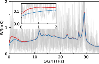
Figure 1: Energy flux of a water-ethanol mixture. Gray: energy-flux sample power spectrum from a $100\,\mathrm{ps}$ trajectory. Red and blue: moving averages over a window of $0.2\,\mathrm{THz}$ of the energy-flux power sample spectrum and of the SCCB of the sample cross-spectrum, computed from a long ($28\,\mathrm{ns}$) trajectory. Inset: low-frequency region of the spectrum.

In order to validate our methodology, we have computed the thermal conductivity of an equimolar water-ethanol mixture. Not aiming at an optimal description of the system, but just at a realistic benchmark, we used the simple OPLSAA Jorgensen et al. (1996) all-atom flexible force field. Classical EMD simulations were run with the LAMMPS package Plimpton (1995) at a temperature of $\approx 350\,\mathrm{K}$ and a density of $0.80\,\mathrm{g/cm^{3}}$, corresponding to $800+800$ molecules in a cubic cell with an edge of $47.47\,\mathrm{{\mbox{\AA}}}$.

In Fig. 1 we report the energy-flux spectrum of our water-ethanol model. The gray line indicates the diagonal element of the raw sample spectrum, computed from a $100\,\mathrm{ps}$ trajectory, which is too noisy to be used as an estimator. Performing a moving average Weisstein (b) of the sample spectrum would consistently reduce the noise, at the price however of requiring much longer trajectories (the blue line reports an average performed from a $28\,\mathrm{ns}$ trajectory) and introducing a bias that is difficult to evaluate and remove. Note that while at high frequency, where the spectrum is dominated by intra-molecular vibrations, the energy-energy diagonal element of the cross-spectrum (red line) and the SCCB coincide, in the low-frequency region, which is characterized by a strongly diffusive behavior, the two differ markedly and only the latter is meaningful to estimate $\kappa$. In Fig. 2 we report the thermal conductivity of the water-ethanol solution computed from Eq. (4) as a function of the upper limit of integration in Eq. (2), and as obtained from a $100\,\mathrm{ps}$ EMD trajectory. The spikes in the estimated conductivity result from the vanishing of the $\Lambda^{11}$ denominator in Eq. (4), which is in turn due to the fact that the integrals of the correlation functions in Eq. (2) behave as random walks as soon as the integrand vanishes, eventually assuming any value. This behavior can be partially corrected by replacing the GK estimate of the Onsager coefficients through Eq. (2) with an equivalent one, based on the Einstein-Helfand relation Baroni et al. (2018); Helfand (1960), which is statistically better behaved (orange line): $\Lambda^{ij}=\lim_{\tau\to\infty}\frac{V}{2k_{B}\tau}\left\langle\int_{0}^{\tau}\mathcal{J}^{i}(t)dt\;\int_{0}^{\tau}\mathcal{J}^{j}(t)dt\right\rangle$. Even so, the statistical accuracy that can be achieved with even longer trajectories is totally inadequate.

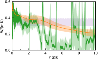
Figure 2: Thermal conductivity of a water-ethanol solution, Eq. (4), as a function of the upper limit of integration in Eq. (2). The shaded areas indicate the estimated statistical error. Green: direct estimate from from Eqs. (4) and (2). Orange: estimate from the Einstein-Helfand relation, see main text. Purple: cepstral analysis estimate.

Cepstral analysis was performed over a $100\,\mathrm{ps}$ EMD trajectory using the ThermoCepstrum open-source code, which is freely available for download Ercole and Bertossa (2018). We set $\ell=3$ (Cartesian components) and $M=2$ (number of conserved fluxes), thus obtaining $L_{0}=\psi(2)-\log(2)\approx-0.270$ and $\sigma_{0}^{2}=\psi^{\prime}(2)\approx 0.644$. The cutoff frequency Ercole et al. (2017) used for cepstral analysis, and ensuring convergence in $\kappa$, was $\omega^{*}/2\pi\approx 35\,\mathrm{THz}$. The number of cepstral coefficients $P^{*}\approx 45$ was estimated from the Akaike Information Criterion Ercole et al. (2017); Akaike (1972); *Akaike1974. The final estimate of the heat conductivity resulting from Eqs. (6) is $\kappa=0.34\pm 0.04\,\mathrm{W/(m\,K)}$. In order to validate our statistical analysis, cepstral analysis was repeated for all the $100\,\mathrm{ps}$ extracted from a $28\,\mathrm{ns}$ long trajectory, confirming the normal distribution of the estimated conductivity and the value of the relative error. The small relative error ($13\%$) achieved by analyzing trajectories as short as $100\,\mathrm{ps}$ shows that cepstral analysis opens the way to heat-transport simulations using ab initio EMD even in multi-component systems. Our analysis equally applies to systems with any number of components in any charge state, because the SCCB is invariant under any nonsingular linear trasformation of the convective fluxes. This implies that in binary molten salts and ionic fluids the electric current, which is a linear combination of mass/number fluxes, can be taken as a proxy of the convective fluxes. An application to molten sodium chloride is presented in the SM Sup .

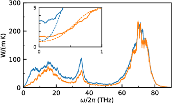
Figure 3: Multi-variate analysis of ab initio water. The sample power spectrum of the DFT energy flux would be out-of-scale and numerically intractable. Blue: SCCB of a two-component analysis performed with the total momentum of the oxygen atoms as an inert flux. Orange: three-component analysis, where the third flux is the electronic adiabatic current. Both are filtered with a moving average of width $1\,\mathrm{THz}$. In the inset, the spectrum obtained from cepstral analysis is displayed in dashed lines.

Multivariate cepstral analysis turns out to be instrumental in heat-transport simulations even for one-component systems. The recently discovered gauge invariance of heat conductivity Marcolongo et al. (2016); Ercole et al. (2016) means that, while transport coefficients are largely independent of the detailed form of the energy flux, the flux power spectrum and the resulting statistical properties of the estimator do depend on it. The question then naturally arises of how to choose the form of the flux so as to optimize these statistical properties. In the case of ab initio water Marcolongo et al. (2016), for instance, the total power of the energy flux derived from density-functional theory (DFT) is so large as to make the statistical analysis of its spectrum at low-frequency intractable, due to large atomic self-energies Marcolongo et al. that cannot be easily defined and eliminated in ab initio simulations. A couple of ad hoc solutions to this problem have been devised Marcolongo et al. (2016, ), leveraging gauge invariance to subtract from the energy flux a linear combination of “inert” fluxes not contributing to heat transport (such as the electronic flux or the mass flux of one of the two atomic species). While this remedy was effective and actually allowed one to get meaningful results from relatively short trajectories, the question remains of how to optimally choose this linear combination. Multivariate cepstral analysis provides the answer. The idea is to compute, along with the energy flux to be analyzed, a number of inert fluxes and treat all of them on a par as though they were conserved fluxes of a multi-component system: the total power of the SCCB will be considerably reduced, thus making the cepstral analysis feasible at low frequency. This is illustrated in Fig. 3, where we report the multi-variate power spectrum of ab initio (heavy) water, computed using the total momentum of the oxygen atoms as an inert flux (blue), as well as this and the adiabatic electronic current as inert fluxes (orange). The simulation setting is the same as in Ref. 12. The spectrum of the bivariate SCCB is always larger than the trivariate one. Using cepstral analysis, the zero-frequency limits of these two spectra coincide, as they must, whereas their running averages do not and depend sensitively on the width of the frequency window. The heat conductivities estimated by cepstral analysis are $(0.74\pm 0.16)\,\mathrm{W/(m\,K)}$ and $(0.69\pm 0.18)\,\mathrm{W/(m\,K)}$, respectively, while the experimental value is $0.61\,\mathrm{W/(m\,K)}$ Matsunaga and Nagashima (1983).

We conclude by noticing that the combination of the newly devised convective invariance and multivariate cepstral analysis, besides providing fresh theoretical insight in transport phenomena, will hopefully broaden the scope of heat-transport simulations to complex multi-component fluids, as well as provide new tools to make ab initio simulations possible.