Auto-Calibration of Cone Beam Geometries
from Arbitrary Rotating Markers using a
Vector Geometry Formulation of Projection Matrices

Abstract

A method for the determination of the projection geometry of highly magnifying cone beam micro computed tomography systems based on few rotating fiducial markers of unknown position within the field of view is derived. By employing the projection matrix formalism commonly used in computer graphics, a very clear presentation of the resulting self consistent calibration problem can be given relating the sought-for matrix to observable parameters of the markers’ projections. Both an easy to implement solution procedure for both the unknown projection matrix and the marker assembly as well as the mapping from projection matrices to real space positions and orientations of source and detector relative to the rotational axis are provided.

The separate treatment of the calibration problem in terms of projection matrices on the one hand and the independent transformation to a more intuitive geometry representation on the other hand proves to be very helpful with respect to the discussion of the ambiguities occurring in reference-free calibration. In particular, a link between methods based on knowledge on the sample and those based on knowledge solely on the detector geometry can be drawn. This further provides another intuitive view on the often reported difficulty in the estimation of the detector tilt towards the rotational axis.

A simulation study considering $10^{6}$ randomly generated cone beam imaging configurations and fiducial marker distributions within a range of typical scenarios is performed in order to assess the stability of the proposed technique.

Lehrstuhl für Röntgenmikroskopie, Physikalisches Institut, Universität Würzburg
Fraunhofer IIS, Division EZRT, Department MRB
Josef-Martin-Weg 63, 97074 Würzburg, Germany

1 Introduction

The determination of the actual – in contrast to the intended – projection geometry within an X-ray cone beam computed tomography system is a common problem to be solved prior to tomographic volume reconstruction. In particular for high resolution micro computed tomography systems, due to the very small source–object distances required for large magnification factors, external determination of the exact geometry is usually difficult given its high sensitivity to small variations in the sample position with respect to the source. It is for this reason generally desirable to determine the actual projection geometry using the system’s immanent imaging capabilities, and most commonly, sparse assemblies of opaque markers that can be individually segmented within projections thereof are used for this purpose.

1.1 Motivation and contribution of the present work

The objective of the present work is to present a simple solution to the cone beam CT auto-calibration problem based on rotating fiducial markers of unknown position on the one hand and to provide intuitive insights into the problem, its solution and its limitations on the other hand. In contrast to the previous work on CBCT auto-calibration, the calibration problem will be formulated in terms of projection matrix elements with the problem of conversion between projection matrices and real space geometry definition being treated separately. It will turn out that this leads to a very clear view on the calibration problem avoiding the cumbersome trigonometric relations between classic geometry parametrizations and the perspective projections of points in 3D space. In particular, the use of generic least squares optimization is largely avoided. The consideration of constraints (i.e., prior knowledge) on either the calibration structure or the projection system takes the form of homography transformations and is separated as an individually solvable problem, rendering the method more general. This allows straight forward extensions to different kinds of prior knowledge, which becomes a matter of constraining the remaining degrees of freedom in the homography matrix, without touching the initial procedure solving the calibration equations.

The present article is structured as follows: First, an overview over related literature on marker based geometry calibration will be given, providing context and motivation for the present work. A very brief introduction to homogeneous coordinates and the projection matrix formalism will be given. A small set of linear equations relating both the unknown projection matrix elements and the parameters of the circular marker trajectories to observable parameters emerges almost directly from the projection matrix based forward model of the projection of rotating points. The following section introduces transformations between projection matrices and real space vector geometry, which provide important insights with respect to constraining the ambiguities arising within auto-calibration. Explicit algorithms implementing the derived strategies are given in the appendix. Finally, a simulation study will be presented, assessing the stability of the procedure on noisy projections of randomly generated sets of projection geometries and marker placements.

1.2 Literature review

1.2.1 Classification of different approaches

Two general classes of approaches can be identified: those based on precisely defined or known marker assemblies [RougeeTrousset1993, Rizo1994, DeMenthonDavis1995, NavabGraumann1996, StrobelWiesent2003, Cho2005, StrubelNoo2005, KYangBoone2006, HoppeNooHornegger2007, MaoXing2008, JohnstonBadea2008, RobertMainprize2009, MennessierClackdoyleNoo2009, XLiBLiu2010, FordWilliamson2011, MXuDLi2014, ZechnerSteiniger2016], which allow calibration on a per-view basis, and those working with fiducials of unknown placement yet requiring precise circular motion of these markers throughout a tomographic scan [Gullberg1990, JLiColeman1993, Noo2000, Smekal2004, KYangBoone2006, WangTsui2007, DWuYXiao2011, GrossSchwanecke2012, SawallKachelriess2012, XuTsui2013, GLi2019] (with some of these assuming the distances between markers known [Noo2000, KYangBoone2006, WangTsui2007, DWuYXiao2011, XuTsui2013]). While the former methods are typically used for macroscopic systems with fields of view in the range of 10 cm and larger, the latter are required for microscopic systems for which the manufacturing of well-defined calibration phantoms is hard to impossible. [Beque2003] assumes both known markers and perfect rotation, and [DefriseNuyts2008] provides a method to account for deviations from expected precise motions, enabling per-view calibration also for methods originally assuming stable circular motions.

An additional distinction can be made from the technical point of view of system parametrization: methods aiming to determine the projective mapping from 3D to 2D space in terms of a projection matrix that is consistent with the available observations irrespective of the question how the particular mapping arises physically [RougeeTrousset1993, NavabGraumann1996, StrobelWiesent2003, StrubelNoo2005, HoppeNooHornegger2007, XLiBLiu2010], and methods aiming to relate projections or properties thereof to real space geometry parameters (relative distances and orientation angles of source and detector) [Gullberg1990, JLiColeman1993, RougeeTrousset1993, Rizo1994, Noo2000, Beque2003, Smekal2004, Cho2005, KYangBoone2006, MaoXing2008, JohnstonBadea2008, RobertMainprize2009, MennessierClackdoyleNoo2009, FordWilliamson2011, DWuYXiao2011, GrossSchwanecke2012, SawallKachelriess2012, XuTsui2013, MXuDLi2014, GLi2019]. Differences also exist in the evaluation of the projection data used for calibration: methods directly working on extracted projection samples (2D points) without further data reduction or interpretation [Gullberg1990, JLiColeman1993, RougeeTrousset1993, DeMenthonDavis1995, NavabGraumann1996, Beque2003, StrobelWiesent2003, HoppeNooHornegger2007, MaoXing2008, SawallKachelriess2012, ZechnerSteiniger2016, GLi2019], as well as methods reducing the observed projections by means of matching them to an expected model (such as e.g. elliptic trajectories) or otherwise exploiting specific geometric features of the utilized calibration structure [Rizo1994, Noo2000, Smekal2004, Cho2005, StrubelNoo2005, KYangBoone2006, JohnstonBadea2008, RobertMainprize2009, MennessierClackdoyleNoo2009, FordWilliamson2011, DWuYXiao2011, GrossSchwanecke2012, XuTsui2013, MXuDLi2014]. Calibration methods may further be characterized based on their core calibration approaches: [RougeeTrousset1993, NavabGraumann1996, StrobelWiesent2003, StrubelNoo2005, HoppeNooHornegger2007, XLiBLiu2010] reduce the calibration problem to the solution of a linear system of equations in a least squares sense e.g. by means of singular value decomposition (requiring the imaged object to be known). [Noo2000, Smekal2004, Cho2005, KYangBoone2006, MennessierClackdoyleNoo2009, XuTsui2013, MXuDLi2014] derive direct relations between parameters of the observed marker patterns and the underlying projection geometry. [Gullberg1990, JLiColeman1993, RougeeTrousset1993, Beque2003, WangTsui2007, ZechnerSteiniger2016] use local optimization techniques requiring sufficiently good initial estimates and [MaoXing2008, GrossSchwanecke2012, SawallKachelriess2012, GLi2019] rely on global optimization techniques for the solution of the inverse problem (also requiring initial estimates). Combinations are used e.g. in [Rizo1994, DeMenthonDavis1995, JohnstonBadea2008, RobertMainprize2009], and a comparison of a matrix inversion and an optimization based approach is given by [RougeeTrousset1993]. Finally, the cited methods differ in the amount of degrees of freedom that are addressed. While methods based on fully known reference objects are generally able to determine all system parameters with reasonable precision, the situation is more complex when no or only few assumptions can be made on the calibration structure.

1.2.2 Review of previous auto-calibration techniques

The early methods addressing the problem of calibration from unknown markers with straight forward least squares minimization approaches considered only the focal distance and the most relevant translations of the detector and the rotational axis [Gullberg1990, JLiColeman1993] due to the instability of the full optimization problem. Noo et al. [Noo2000] showed that generic optimization can be largely avoided by systematic analysis of the problem. By constraining the detector columns parallel to the rotational axis, they were able to derive relations between the remaining geometric parameters and the ellipse parameters of the observable projections of two opaque markers moving along circular trajectories around the rotational axis. Potential detector in-plane rotations are considered in an independent preprocessing step. They assumed the distance between the markers known in order to determine also the absolute scale. The method was further simplified by Yang et al. [KYangBoone2006] for the case of also negligible detector slant about the rotational axis. Johnston et al. [JohnstonBadea2008] use the latter approximate approach for the initialization of a generic local optimization procedure that is then able to recover all parameters using a phantom of ten collinear bearing balls with defined distances. A further adaption of the Noo method was presented by [DWuYXiao2011]. Bequé et al. [Beque2003, Beque2005] and Wang and Tsui [WangTsui2007] fully revert to local optimization again yet analyze the uniqueness of general solutions based on one, two and three rotating markers and conclude that one known distance between two markers is sufficient in the presence of detector slant about the rotational axis, and two known distances (which they relate to distances between three markers) are required for a generally unique solution for all system parameters, which was also conjectured previously by Noo et al. [Noo2000] and is also stated by Xu and Tsui [XuTsui2013]. In the related methods addressing all system parameters based on two known parallel rings (of equal radius) of bearing balls by Cho et al. [Cho2005] and Robert et al. [RobertMainprize2009], this condition is fulfilled by knowledge of both the vertical distance of those circles and their (common) radius. Further Xu and Tsui [XuTsui2013] propose another calibration procedure based on relations between elliptical projections of rotating markers, known marker distances and the system geometry, yet in contrast to [Noo2000, KYangBoone2006, RobertMainprize2009] identify geometrically meaningful intersection points on the ellipses in the style of the approaches by Cho et al. [Cho2005] and Strubel et al. [StrubelNoo2005] (who worked with fully known structures) in order to then obtain simpler relations between those points in the projection image and the geometry parameters. A general methodology for the assessment of uniqueness and stability of calibration problems by means of analyzing the propagation of random errors through the respective forward model has been discussed by Ma et al. [TMa2009].

Smekal et al. [Smekal2004] were, to the author’s knowledge, the first to explicitly address the case of complete auto-calibration (up to an unknown object scale, yet including detector tilt) of cone beam tomography systems based on multiple rotating markers at unknown positions and distances. The latter were either required or assumed known in the methods discussed so far. They choose a different parametrization for the analysis of the projected circles more directly related to the forward model than the otherwise often used ellipse equation and are able to find relations of those observable parameters to all geometric parameters. In contrast to the previous literature, Smekal et al. conclude that one marker is, in principle, sufficient for all parameters but tilt (and absolute scale). In accordance with previous literature they find that at least two projected trajectories (yet without knowledge of the marker’s distance) are required to infer tilt provided that the detector is also slanted about the rotational axis. They do not further investigate the case of zero slant. In their experiments, they use between eight and twelve markers and average the obtained geometry parameters.

The more recent publications by Gross et al. [GrossSchwanecke2012], Sawall et al. [SawallKachelriess2012] and Li et al. [GLi2019] also consider the problem of complete auto-calibration (up to an unknown scale) without reverting to known sample properties, although all, in contrast to Smekal, require global optimization techniques.

Gross et al. [GrossSchwanecke2012] formulate the problem in terms of a homography transform parametrized by the sought-for system properties relating the observable ellipses to a canonical representation of circular trajectories. They were thereby able to eliminate the trajectory parameters from the optimization problem, reducing it to 6 degrees of freedom describing the projection geometry (in comparison, Robert et al. [RobertMainprize2009] previously reported a reduction of the optimization problem relating ellipse parameters and geometry parameters to 3 dimensions for the case of known trajectory parameters). As has been the case also with previous techniques based on ellipse analysis [Noo2000, Cho2005, StrubelNoo2005, KYangBoone2006, RobertMainprize2009, DWuYXiao2011, XuTsui2013], the evaluated ellipses are expected to be non-degenerate in order to successfully reconstruct the projection geometry. In their experiments, they use between three and twelve markers and generally recommend the use of more than four non-degenerate ellipses for their method.

Sawall et al. [SawallKachelriess2012] apply a genetic optimization algorithm to a straight-forward objective function penalizing the least squares errors between forward model and observations. Rather than using multiple rotating markers within one tomographic scan, they use a single marker scanned at multiple different geometric configurations of the employed tomography setup. As discussed earlier [Beque2003, WangTsui2007], this provides enough information to simultaneously determine each scan geometry. Sawall et al. were the only ones to actually work with the absolute minimum of one marker, although simultaneous calibration of multiple systems or multiple configurations of the same system has been addressed before [Beque2003, WangTsui2007, JohnstonBadea2008].

Li et al. [GLi2019] likewise use global optimization to relate the forward model to observed marker projections, yet specifically design the cost function to exploit known consistency constraints of two-view geometries. Namely, the lines between focal spot, marker and the marker’s projection on the detector for two views of the same marker must obviously intersect, and do so at the location of the marker. The complete elimination of degrees of freedom to be optimized, as previously shown by Gross et al. [GrossSchwanecke2012], could thereby not be achieved.

In the following, an analytically motivated approach to reference-free calibration will be presented that, in contrast to the ones by Gross et al. [GrossSchwanecke2012], Sawall et al. [SawallKachelriess2012] and Li et al. [GLi2019], does not require the use of generic non-convex optimization techniques, and thus in particular does not require initial estimates for any of the parameters. It is in this respect most similar to the method described by Smekal et al. [Smekal2004]. Other than in [Smekal2004] and other previous approaches, the problem will be parametrized by projection matrix elements, which has previously only been done in the context of known calibration structures (cf. [RougeeTrousset1993, NavabGraumann1996, StrobelWiesent2003, StrubelNoo2005, HoppeNooHornegger2007, XLiBLiu2010]). This will on the one hand allow a very simple representation of the core calibration problem and on the other hand expose the link between methods solely based on constraints on the detector geometry ([Smekal2004, GrossSchwanecke2012, SawallKachelriess2012, GLi2019]) and those based on (partial) prior knowledge on the sample (e.g. [Beque2003, Beque2005, StrubelNoo2005, Cho2005, WangTsui2007, JohnstonBadea2008, RobertMainprize2009, XuTsui2013]).

2 Methods

2.1 Formalization of the calibration task

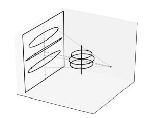
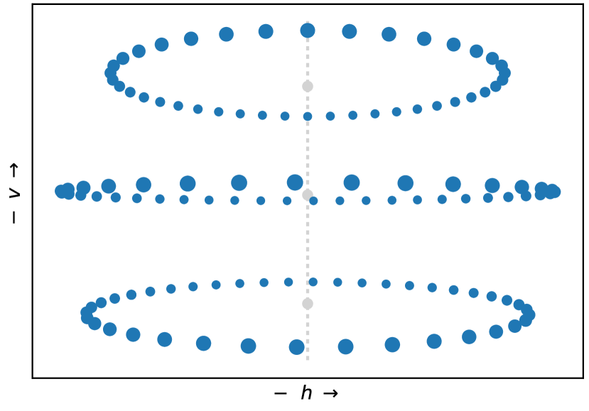
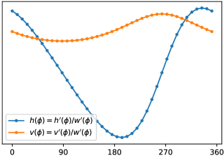
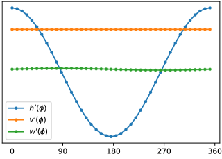
Figure 1: Upper left: Fiducial markers moving along circular trajectories about the rotational axis (center) of a cone beam computed tomography setup, projected by a point source (right) onto a planar detector (left).    Upper right: Superposition of respective projection images on the detector.    Lower left: Horizontal and vertical components of a projected trajectory in dependence of the projection angle $\phi$ (cf. Eqs. 25, 26).    Lower right: Decomposition of the projection components into independent sinusoids describing the orthographic horizontal and vertical projections $h^{\prime}(\phi)$ and $v^{\prime}(\phi)$ as well as the perspective scaling component $w^{\prime}(\phi)$ (cf. Eq. 20).

Figure 2: Depiction of the real space geometry description used here. The world coordinate origin is centered in the field of view and the positions of source ($\vec{s}$) and detector coordinate origin $(\vec{d}$) are defined relative to that. The row and column vectors $\vec{H}$ and $\vec{V}$ characterize the detector orientation and pixel pitches. This vectorial description does not restrict $\vec{H}$ and $\vec{V}$ to be orthogonal or of equal length, although this is a common property of actual imaging systems and will here be used to constrain ambiguities of the auto calibration problem. The 3D world coordinates of a 2D point $(h,v)$ in the planar coordinate system of the detector are given by $\vec{d}+h\vec{H}+v\vec{V}$. The relation to projection matrices is described in Section 2.3.2.

Perspective projections onto planar detectors can generally be expressed in terms of homogeneous coordinates and projection matrices as commonly used in computer graphics. Homogeneous coordinates hold an additional scaling component (here: $w$) defining an equivalence class such that all vectors $(w\,x,\,w\,y,\,w\,z,\,w)$ with $w\neq 0$ describe the same point $(x,y,z)$ [HartleyZisserman2004]. Corresponding euclidean coordinates are obtained by dividing a given homogeneous vector by its scaling component and dropping the latter. While the motivation for this representation will become more clear in Section 2.3.2, it is for now only relevant to know that the 2D cone beam projection $(h(\phi),v(\phi))$ of a circular trajectory $(r\cos(\phi-\phi_{0}),r\sin(\phi-\phi_{0}),z)$ about the $z$-axis can generally be represented as:

$$\left[\begin{array}[]{c}h^{\prime}(\phi)\\ v^{\prime}(\phi)\\ w^{\prime}(\phi)\end{array}\right] =\left[\begin{array}[]{cccc}P_{11}&P_{12}&P_{13}&P_{14}\\ P_{21}&P_{22}&P_{23}&P_{24}\\ P_{31}&P_{32}&P_{33}&P_{34}\end{array}\right]\left[\begin{array}[]{c}r^{\prime}\cos(\phi-\phi_{0})\\ r^{\prime}\sin(\phi-\phi_{0})\\ z^{\prime}\\ w\end{array}\right]$$ (11)

$$h(\phi) =h^{\prime}(\phi)/w^{\prime}(\phi)$$ (12)

$$v(\phi) =v^{\prime}(\phi)/w^{\prime}(\phi)$$ (13)

with

$$r =r^{\prime}/w$$

$$z =z^{\prime}/w\,.$$

$w$ and $w^{\prime}$ are the scaling components of the vector on the right-hand side and its projection on the left-hand side respectively. Although the component $w$ on the right-hand side would, if projections of known points were to be calculated, commonly be defined to equal $1$, it will be beneficial for the purposes of the following derivations to actually leave it as an open parameter. $P_{mn}$ represent the components of a $3\times 4$ projection matrix $\boldsymbol{P}$ encoding the projection geometry, i.e. the placement of source and detector in 3D space as well as the detector pixel pitches. The detailed relation between geometry and projection matrix will be discussed later in Section 2.3.2.

Evaluating the above matrix-vector product and applying trigonometric identities yields

$$\left[\begin{array}[]{c}h^{\prime}(\phi)\\ v^{\prime}(\phi)\\ w^{\prime}(\phi)\end{array}\right] =\left[\begin{array}[]{c}r^{\prime}(P_{11}\cos(\phi-\phi_{0})+P_{12}\sin(\phi-\phi_{0}))+P_{13}z^{\prime}+P_{14}w\\ r^{\prime}(P_{21}\cos(\phi-\phi_{0})+P_{22}\sin(\phi-\phi_{0}))+P_{23}z^{\prime}+P_{24}w\\ r^{\prime}(P_{31}\cos(\phi-\phi_{0})+P_{32}\sin(\phi-\phi_{0}))+P_{33}z^{\prime}+P_{34}w\end{array}\right]$$ (20)

$$=\left[\begin{array}[]{c}r^{\prime}P_{1\mathrm{a}}\sin(\phi-\phi_{0}-\phi_{\mathrm{h}})+P_{13}z^{\prime}+P_{14}w\\ r^{\prime}P_{2\mathrm{a}}\sin(\phi-\phi_{0}-\phi_{\mathrm{v}})+P_{23}z^{\prime}+P_{24}w\\ r^{\prime}P_{3\mathrm{a}}\sin(\phi-\phi_{0}-\phi_{\mathrm{w}})+P_{33}z^{\prime}+P_{34}w\end{array}\right]$$ (24)

with

$$P_{m\mathrm{a}} =\sqrt{P_{m1}^{2}+P_{m2}^{2}}$$

$$\phi_{\mathrm{h}} =\mathrm{arctan}2(-P_{11},P_{12})$$

$$\phi_{\mathrm{v}} =\mathrm{arctan}2(-P_{21},P_{22})$$

$$\phi_{\mathrm{w}} =\mathrm{arctan}2(-P_{31},P_{32})$$

$$\Updownarrow$$

$$P_{m1} =-P_{1\mathrm{a}}\sin(\phi_{m})$$

$$P_{m2} =\phantom{-{}}P_{1\mathrm{a}}\cos(\phi_{m})\>,$$

where $m$ equally enumerates both the rows $(1$, $2$ and $3$) of $\boldsymbol{P}$ as well the associated subscript labels $\mathrm{h}$, $\mathrm{v}$ and $\mathrm{w}$, which have been chosen to clearly indicate the relation of the rows or their respective parameters to the three components of the left-hand side homogeneous vector.

The $h$ and $v$ projection coordinates on the detection plane are thus finally given by:

$$h(\phi) =\frac{r^{\prime}P_{1\mathrm{a}}\sin(\phi-\phi_{0}-\phi_{\mathrm{h}})+P_{13}z^{\prime}+P_{14}w}{r^{\prime}P_{3\mathrm{a}}\sin(\phi-\phi_{0}-\phi_{\mathrm{w}})+P_{33}z^{\prime}+P_{34}w}$$ (25)

$$v(\phi) =\frac{r^{\prime}P_{2\mathrm{a}}\sin(\phi-\phi_{0}-\phi_{\mathrm{v}})+P_{23}z^{\prime}+P_{24}w}{r^{\prime}P_{3\mathrm{a}}\sin(\phi-\phi_{0}-\phi_{\mathrm{w}})+P_{33}z^{\prime}+P_{34}w}\quad.$$ (26)

The numerators in these expressions correspond to the orthographic (“parallel beam”) projection, while the common denominator describes the distance dependent perspective scaling. See Figure 1 for an example.

As in the context of self consistent calibration neither $P_{mn}$ nor $r^{\prime}$, $z^{\prime}$, $\phi_{0}$ and $w$ are known, the above equations may as well be expressed in terms of the independent sinusoid parameters $a_{i\mathrm{h}}$, $a_{i\mathrm{v}}$, $a_{i\mathrm{w}}$, $\phi_{i0\mathrm{h}}$, $\phi_{i0\mathrm{v}}$, $\phi_{i0\mathrm{w}}$, $o_{i\mathrm{h}}$ and $o_{i\mathrm{v}}$ representing amplitudes, phases and offsets respectively and including an additional index $i$ for the enumeration of multiple projected trajectories:

$$h_{i}(\phi) =\frac{a_{i\mathrm{h}}\sin(\phi-\phi_{i0\mathrm{h}})+o_{i\mathrm{h}}}{a_{i\mathrm{w}}\sin(\phi-\phi_{i0\mathrm{w}})+1}$$ (27)

$$v_{i}(\phi) =\frac{a_{i\mathrm{v}}\sin(\phi-\phi_{i0\mathrm{v}})+o_{i\mathrm{v}}}{a_{i\mathrm{w}}\sin(\phi-\phi_{i0\mathrm{w}})+1}\quad.$$ (28)

The determination of these 8 sinusoid parameters for each projected trajectory $i$ is detailed in Section 7.3 (Eqs. 94–104 and Algorithm 2). In the following, they can be considered known.

The calibration problem, i.e. the simultaneous reconstruction of both the unknown projection matrix $\boldsymbol{P}$ and the unknown fiducial marker orbits from given projections $(h_{i}(\phi),v_{i}(\phi)$), can now be identified as the solution of the following linear system of equations relating the observable sinusoid parameters of the projected trajectories to the unknown projection matrix and orbit parameters for all imaged trajectories $i$:

$$r_{i}^{\prime}P_{1\mathrm{a}} =a_{i\mathrm{h}}$$ (29)

$$r_{i}^{\prime}P_{2\mathrm{a}} =a_{i\mathrm{v}}$$ (30)

$$r_{i}^{\prime}P_{3\mathrm{a}} =a_{i\mathrm{w}}$$ (31)

$$P_{13}z_{i}^{\prime}+P_{14}w_{i} =o_{i\mathrm{h}}$$ (32)

$$P_{23}z_{i}^{\prime}+P_{24}w_{i} =o_{i\mathrm{v}}$$ (33)

$$P_{33}z_{i}^{\prime}+P_{34}w_{i} =o_{i\mathrm{w}}=1$$ (34)

$$\phi_{\mathrm{h}} =0$$ (35)

$$\phi_{\mathrm{v}} =\phi_{i0\mathrm{v}}-\phi_{i0\mathrm{h}}$$ (36)

$$\phi_{\mathrm{w}} =\phi_{i0\mathrm{w}}-\phi_{i0\mathrm{h}}$$ (37)

where $\phi_{\mathrm{h}}$ is defined to be $0$, exploiting the freedom of choice of the projection angle for a rotationally symmetric imaging configuration (or equivalently the freedom of choice of the initial phase of a periodic trajectory). Further, the fixed parameter $o_{i\mathrm{w}}=1$ has been introduced in order to maintain a uniform representation of the equations. For the same reason, the subscripts “h”, “v” and “w” will in the following as well be represented by the projection matrix’ row index $m$, i.e. $\mathrm{h}\,\widehat{=}\,1,\mathrm{v}\,\widehat{=}\,2,\mathrm{w}\,\widehat{=}\,3$. A practical method for the solution of the above calibration equations is described in Section 7.2.

2.2 Projective ambiguties

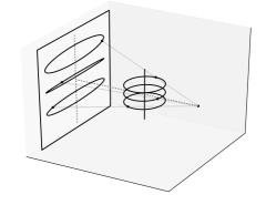
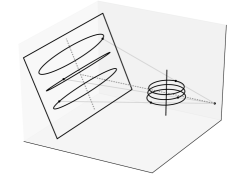
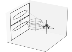
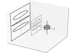
Figure 3: Examples of projective ambiguity: the same projections $(h(\phi),v(\phi))$ may originate from different combinations of imaging configuration and marker locations. The top row illustrates the effect of $\boldsymbol{D}(\delta=1,\gamma\neq 0)$, while the bottom row shows examples of $\boldsymbol{S}$ with the effects of the parameters $s_{\mathrm{o}}$ (bottom left) and $s_{\mathrm{d}}$ (bottom right) respectively (cf. Eqs. 38–62). The latter case corresponds to the general scaling degree of freedom of homogeneous projection matrices.

The given equations further reveal that the first two and last two columns of $\boldsymbol{P}$ are independent, i.e. there are no equations interrelating these parts of the projection matrix (Eqs. 29–31 are independent from Eqs. 32–34). Similarly, the relation between $z_{i}^{\prime}$ and $w_{i}$ and consequently the third and fourth column of $\boldsymbol{P}$ is not unique (cf. Eqs. 32–34). Together with the ambiguities expected by design, i.e., arbitrary choice of length units, object scale and related source–object distance, definition of the $\phi=0{{}^{\circ}}$ orientation within the $x$-$y$ plane and the choice of origin on the $z$-axis, these ambiguities are a special case of general projective ambiguities of the form

$$\boldsymbol{P}\vec{x}=\boldsymbol{P}\boldsymbol{H}^{-1}\boldsymbol{H}\vec{x}=(\boldsymbol{P}\boldsymbol{H}^{-1})(\boldsymbol{H}\vec{x})=\tilde{\boldsymbol{P}}\tilde{\vec{x}}\>,$$ (38)

with the homography $\boldsymbol{H}$ being composed of the following transformations in the present case:

$$\boldsymbol{H}^{\phantom{-1}} =\boldsymbol{R}_{z}(\omega)\,\boldsymbol{T}_{z}(\Delta z)\,\boldsymbol{S}(s_{\mathrm{d}},s_{\mathrm{o}})\,\boldsymbol{D}(\delta,\gamma)$$ (39)

$$\boldsymbol{H}^{-1} =\boldsymbol{D}^{-1}(\delta,\gamma)\,\boldsymbol{S}(s_{\mathrm{d}}^{-1},s_{\mathrm{o}}^{-1})\,\boldsymbol{T}_{z}(-\Delta z)\,\boldsymbol{R}_{z}(-\omega)\>,$$

with

$$\boldsymbol{R}_{z}(\omega) =\left[\begin{array}[]{cccc}\cos(\omega)&-\sin(\omega)&0&0\\ \sin(\omega)&\phantom{-}\cos(\omega)&0&0\\ 0&0&1&0\\ 0&0&0&1\end{array}\right] \boldsymbol{T}_{z}(\Delta z) =\left[\begin{array}[]{cccc}1&0&0&0\\ 0&1&0&0\\ 0&0&1&\Delta z\\ 0&0&0&1\end{array}\right]$$ (48)

$$\boldsymbol{S}(s_{\mathrm{d}},s_{\mathrm{o}}) =s_{\mathrm{d}}\left[\begin{array}[]{cccc}1&0&0&0\\ 0&1&0&0\\ 0&0&1&0\\ 0&0&0&s_{\mathrm{o}}\end{array}\right]$$ (53)

$$\boldsymbol{D}(\delta,\gamma) =\left[\begin{array}[]{cccc}1&0&0&0\\ 0&1&0&0\\ 0&0&1/\text{$\delta$}&0\\ 0&0&\gamma&1\end{array}\right] \boldsymbol{D}^{-1}(\delta,\gamma) =\left[\begin{array}[]{cccc}1&0&0&0\\ 0&1&0&0\\ 0&0&\text{$\delta$}&0\\ 0&0&-\delta\gamma&1\end{array}\right]\>.$$ (62)

Rotation $\boldsymbol{R}_{z}(\omega)$, $z$-translation $\boldsymbol{T}_{z}(\Delta z)$ and gobal scale $s_{\mathrm{d}}$ correspond to a choice of reference frame and length unit that can be made at the users convenience. The object scale $s_{\mathrm{o}}$ affects both the object size and the relation between source–axis and detector–axis distance accordingly and can only be determined based on prior knowledge on the sample and will therefore be arbitrarily fixed to $s_{\mathrm{o}}=1$ here. $\boldsymbol{D}(\delta,\gamma)$ describes the initially mentioned independence of Eqs. 29–31 and Eqs. 32–34 and affects the object and detector geometry respectively and is therefore of particular interest here. Examples of the ambiguities described by $\boldsymbol{D}$ and $\boldsymbol{S}$ are depicted in Figure 3.

In contrast to the other transformations, $\boldsymbol{D}(\delta,\gamma)$ can be constrained by drawing upon further knowledge on the imaging system, whose pixel aspect ratio as well as the angle between detector rows and columns is commonly known. Anticipating the derivations given in Sections 7.1.1–7.1.2, it can be summarized that $\delta$ affects the detector pixel aspect ratio, while $\gamma$ simultaneously affects the pixel shear, aspect ratio and the tilt angle of the detector plane. With $\gamma=0$, $\delta$ may be chosen according to Equation 86 in order to enforce a given detector pixel aspect ratio, whereby $\varepsilon=1$ for many typical detectors. Otherwise, $\gamma$ and $\delta$ need to be determined simultaneously by optimization of an objective function as defined by Equation 87 which approaches $0$ for rectangular detector pixels (i.e., $\vec{H}\cdot\vec{V}=0$) of aspect ratio $\varepsilon$ (i.e., $\bigl{\|}\vec{H}\bigr{\|}/\bigl{\|}\vec{V}\bigr{\|}=\varepsilon$). In the case of zero detector slant about the rotational axis, Equation 87 has no unique minimum and therefore many solutions for $\gamma$ and $\delta$. This degeneracy of auto calibration with respect to detector tilt has also been described e.g. by Smekal et al. [Smekal2004] and can further be related to the general difficulty to precisely determine detector tilt, which has been reported in context of many different calibration approaches.

Besides constraints on the detector geometry, knowledge on the sample such as relative distances between markers (as often used in previous literature) could be used as well in order to determine the two parameters defining $\boldsymbol{D}$. This however shall not be further considered here given the specific focus on calibration based on unknown marker locations.

2.3 Relation between Real Space Geometry and Projection Matrices

With respect to the final objective to conversely transform projection matrices to real space vectors describing source and detector location as well as detector row and column orientations (see Figure 2), first the formulation of projection matrices in terms of real space geometry vectors will be discussed. The derived relations between projection matrices and vector geometries will be required both for the resolution of projective ambiguities and for general real space interpretations of the calibration results.

2.3.1 Formulation of Projection Matrices in Terms of Vector Geometry

To begin with, a vectorial formulation of the rays running between source and detector shall be given to this end: An euclidean point $\vec{p}$ somewhere on the connecting line between source $\vec{s}$ and a detector pixel $(\vec{d}+h\vec{H}+v\vec{V})$ characterized by the detector location $\vec{d}$, the pixel’s coordinate $(h,v)$ on the detector matrix and the detector row and column strides $\vec{H}$ and $\vec{V}$ relating the matrix to real space, is described by the parametric equation

$$\vec{p}(h,v,w)=\vec{s}+w\underbrace{\Bigl{(}(\overbrace{\vec{d}+h\vec{H}+v\vec{V}}^{\mathclap{\begin{subarray}{c}\text{position of pixel }(h,v)\\ \text{in 3D space}\end{subarray}}})-\vec{s}\Bigr{)}}_{\text{line orientation}}$$ (63)

with $w$ characterizing the relative position along the line between source $\vec{s}$ and detector pixel $(\vec{d}+h\vec{H}+v\vec{V})$.

The projection $(h,v)$ of a given point $\vec{p}$ is given by the inverse of the above relation. By choice of a more convenient representation of Eq. 63 introducing the auxiliary variables $h^{\prime}$ and $v^{\prime}$, the inversion can be formulated as follows:

$$\vec{p} =\vec{s}+\overbrace{w\,h}^{\smash[t]{h^{\prime}}}\vec{H}+\overbrace{\vphantom{h}w\,v}^{\smash[t]{v^{\prime}}}\vec{V}+w\,(\vec{d}-\vec{s})$$ (64)

$$\vec{p}-\vec{s} =\left[\begin{array}[]{c}\!\vec{H}\>\Bigl{|}\>\vec{V}\>\Bigr{|}\>\vec{d}-\vec{s}\end{array}\right]\left[\begin{array}[]{c}\!h\mathrlap{{}^{\prime}}\!\\ \!v\mathrlap{{}^{\prime}}\!\\ \!w\!\end{array}\right]$$ (69)

$$\smash[t]{\left[\begin{array}[]{c}\!h\mathrlap{{}^{\prime}}\!\\ \!v\mathrlap{{}^{\prime}}\!\\ \!w\!\end{array}\right]} =\left[\begin{array}[]{c}\!\vec{H}\>\Bigl{|}\>\vec{V}\>\Bigr{|}\>\vec{d}-\vec{s}\end{array}\right]^{-1}\Bigl{[}\vec{p}-\vec{s}\,\Bigr{]}$$ (74)

$$\left[\begin{array}[]{c}h\\ v\end{array}\right] =\frac{1}{w}\left[\begin{array}[]{c}h^{\prime}\\ v^{\prime}\end{array}\right]\>.$$ (79)

This solution to the problem $(h(\vec{p}),v(\vec{p}))$ can be straight forwardly reformulated to reproduce the projection matrix formalism:

$$\overbrace{\negthickspace\negthickspace\left[\begin{array}[]{c}h\mathrlap{{}^{\prime}}\\ v\mathrlap{{}^{\prime}}\\ w\end{array}\right]\negthickspace\negthickspace}^{\mathclap{\begin{subarray}{c}2\mathrm{D}+1\text{ homoge-}\\ \text{neous coordinate}\end{subarray}}}\;\>=\Bigl{[}\,\overbrace{\underbrace{\Bigl{[}\begin{array}[]{c}\!\vec{H}\>\Bigl{|}\>\vec{V}\>\Bigr{|}\>\vec{d}-\vec{s}\end{array}\Bigr{]}^{-1}}_{\boldsymbol{P}_{3\times 3}}\>\Bigr{|}\>\underbrace{\Bigl{[}\begin{array}[]{c}\!\vec{H}\>\Bigl{|}\>\vec{V}\>\Bigr{|}\>\vec{d}-\vec{s}\end{array}\Bigr{]}^{-1}\Bigl{[}-\vec{s}\,\Bigr{]}}_{\boldsymbol{P}_{4}}\,}^{3\times 4\text{ projection matrix }\text{$\boldsymbol{P}$}}\Bigr{]}\Bigl{[}\overbrace{\begin{array}[]{c}\vec{p}\\ 1\end{array}}^{\mathclap{\begin{subarray}{c}3\mathrm{D}+1\\ \text{homogeneous}\\ \text{coordinate}\end{subarray}}}\Bigr{]}\>,$$ (80)

where the remaining constant ($\vec{s}$) of the projection geometry has been included within the fourth column ($\boldsymbol{P}_{4}$) of the projection matrix $\boldsymbol{P}$. By means of the corresponding fourth component added to the to-be-projected point $\vec{p}$, the projection matrix formalism exactly reproduces Eq. 74. All constants of the projection geometry are now completely contained within $\boldsymbol{P}$, and the projection takes the form of a linear map between homogeneous coordinates. An explicit representation of $\boldsymbol{P}$ is found by application of Cramer’s rule:

$$\begin{aligned} \boldsymbol{P}&=\alpha\left[\begin{array}[]{c}\phantom{-}(\phantom{\vec{H}}\mathllap{\vec{V}}\times(\vec{d}-\vec{s}))^{T}\\ -(\vec{H}\times(\vec{d}-\vec{s}))^{T}\\ \phantom{-}(\vec{H}\times\mathrlap{\vec{V}}\phantom{(\vec{d}-\vec{s})})^{T}\end{array}\left|\begin{array}[]{c}-(\phantom{\vec{H}}\mathllap{\vec{V}}\times\mathrlap{\vec{d}}\phantom{\vec{V}})\cdot\vec{s}\\ \phantom{-}(\vec{H}\times\mathrlap{\vec{d}}\phantom{\vec{V}})\cdot\vec{s}\\ -(\vec{H}\times\vec{V})\cdot\vec{s}\end{array}\right.\right]\\ \text{with}\quad\alpha&=\det\left(\Bigl{[}\begin{array}[]{c}\!\vec{H}\>\Bigl{|}\>\vec{V}\>\Bigr{|}\>\vec{d}-\vec{s}\end{array}\Bigr{]}\right)^{-1}=\left((\vec{H}\times\vec{V})\cdot(\vec{d}-\vec{s})\right)^{-1}\>,\end{aligned}$$ (81)

where the determinant $\alpha$ can, due to the invariance of projections with respect to the absolute scale of $\boldsymbol{P}$, be dropped for all practical purposes. It is here explicitly included for consistency with Eq. 80.

2.3.2 Conversion of Projection Matrices to Real Space Vectors

Based on the representation given in Eqs. 80, the relation

$$\vec{s}=-\boldsymbol{P}_{3\times 3}^{-1}\boldsymbol{P}_{4}$$ (82)

can be directly inferred, with $\vec{s}$ being the focal point of the projection. As can be easily verified, Eq. 82 is invariant with respect to the absolute scale of $\boldsymbol{P}$.

The remaining vectors $\vec{H}$, $\vec{V}$ and $\vec{d}$ are, in contrast, related to the absolute scale of $\boldsymbol{P}$. The ambiguity corresponds to the fact that projections in the coordinate system of the detection screen are invariant under a proportional change of scale and distance of that screen, as well as under reflection through the focal point. In order to recover the screen’s actual scale from an arbitrarily normalized matrix $\boldsymbol{P}$, prior knowledge such as the true pixel pitch $\bigl{\|}\vec{H}\bigr{\|}$ or $\bigl{\|}\vec{V}\bigr{\|}$ and the screen’s orientation with respect to $\vec{s}$ needs to be incorporated. Nevertheless, a valid preliminary set of equivalent vectors $\vec{H}^{\prime}$, $\vec{V}^{\prime}$ and $\vec{d}^{\prime}$ reproducing a given projection matrix $\boldsymbol{P}$ can generally be obtained irrespective of the original system dimensions based on Eqs. 80 and 82:

$$\Bigl{[}\begin{array}[]{c}\!\vec{H}^{\prime}\>\Bigl{|}\>\vec{V}^{\prime}\>\Bigr{|}\>\vec{d}^{\prime}-\vec{s}\end{array}\Bigr{]}=\boldsymbol{P}_{3\times 3}^{-1}$$ (83)

Based on the assumption typical to X-ray imaging that $(\vec{d}-\vec{s})\cdot\vec{s}<0$, i.e., that the focal point never lies between the projected field of view and the projection screen, and further assuming the pixel pitches $\bigl{\|}\vec{H}\bigr{\|}$ and $\bigl{\|}\vec{V}\bigr{\|}$ to be known, Equations 82 and 83 may be completed to

$$\vec{s} =-\boldsymbol{P}_{3\times 3}^{-1}\boldsymbol{P}_{4}$$ (84)

$$\Bigl{[}\begin{array}[]{c}\!\vec{H}^{\prime}\>\Bigl{|}\>\vec{V}^{\prime}\>\Bigr{|}\>\vec{d}^{\prime}-\vec{s}\end{array}\Bigr{]} =\phantom{-}\boldsymbol{P}_{3\times 3}^{-1}$$

$$\Bigl{[}\begin{array}[]{c}\!\mathrlap{\vec{H}}\phantom{\vec{H}^{\prime}}\>\Bigl{|}\>\mathrlap{\vec{V}}\phantom{\vec{V}^{\prime}}\>\Bigr{|}\>\mathrlap{\vec{d}}\phantom{\vec{d^{\prime}}}-\vec{s}\end{array}\Bigr{]} =-\mathrm{sign}((\vec{d^{\prime}}-\vec{s})\cdot\vec{s})\smash{\sqrt{\frac{\bigl{\|}\vec{H}\bigr{\|}}{\bigl{\|}\vec{H}^{\prime}\bigr{\|}}\frac{\bigl{\|}\vec{V}\bigr{\|}}{\bigl{\|}\vec{V}^{\prime}\bigr{\|}}}}\Bigl{[}\begin{array}[]{c}\!\vec{H}^{\prime}\>\Bigl{|}\>\vec{V}^{\prime}\>\Bigr{|}\>\vec{d}^{\prime}-\vec{s}\end{array}\Bigr{]}$$

$$\vec{d} =(\vec{d}-\vec{s})+\vec{s}\>,$$

whereby the geometric mean over both pixel pitches is meaningful in the presence of noise on $\vec{H}^{\prime}$ and $\vec{V}^{\prime}$, as will be the case when $\boldsymbol{P}$ is actually determined from experimental data instead of being explicitly constructed. With respect to the discussion of projective ambiguities (Sections 2.2 and 7.1) it is further insightful to explicitly state the inverse $\boldsymbol{P}_{3\times 3}^{-1}$ using Cramer’s rule:

$$\vec{H}\propto\quad\hphantom{(\vec{d}^{\prime}-\vec{s})}\mathllap{\vec{H}^{\prime}} =\hphantom{-}\alpha^{-1}\,(P_{21},P_{22},P_{23})\times(P_{31},P_{32},P_{33})$$ (85)

$$\vec{V}\propto\quad\hphantom{(\vec{d}^{\prime}-\vec{s})}\mathllap{\vec{V}^{\prime}} =-\alpha^{-1}\,(P_{11},P_{12},P_{13})\times(P_{31},P_{32},P_{33})$$

$$(\vec{d}-\vec{s})\propto\quad(\vec{d}^{\prime}-\vec{s}) =\hphantom{-}\alpha^{-1}\,(P_{11},P_{12},P_{13})\times(P_{21},P_{22},P_{23})$$

$$\alpha =\det\boldsymbol{P}_{3\times 3}=[(P_{11},P_{12},P_{13})\times(P_{21},P_{22},P_{23})]\cdot(P_{31},P_{32},P_{33})$$

$$\alpha^{-1} =\det\boldsymbol{P}_{3\times 3}^{-1}=(\vec{H}^{\prime}\times\vec{V}^{\prime})\cdot(\vec{d}^{\prime}-\vec{s})\quad(\text{cf. also Eq. }\ref{eq:pmat-explicit})$$

3 Simulation Study

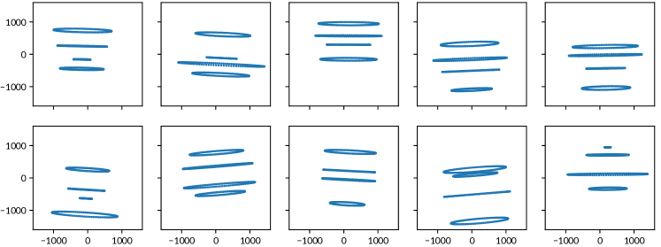
Figure 4: Examples of simulated projections of rotating fiducial markers as used to quantify the auto calibration precision. Both the projection geometry and the marker placement are randomly generated. Positions are given in units of detector pixels, with the origin defined in the detector’s center. Auto calibration is performed both from all shown trajectories (4 markers) as well as from only the top and bottom ones (2 markers). Cf. Fig. 5.

The calibration procedure has been tested on simulations of a large set of randomly generated imaging configurations and fiducial marker positions in order to obtain information on the average precision independent of the particular projection geometry or calibration phantom. The random samples are generated from both a mean imaging configuration and mean phantom shape with broad variances on the actual positions and orientations. In units of detector pixels, detectors with roughly 1500 to 3000 pixels width and 1000 to 2000 pixels height at a source–detector distance of 10000 times the detector pixel size are modeled, yielding cone angles in the range of about $(12\pm 5){{}^{\circ}}$. With the rotational axis virtually placed at the location of the detector, also the sample units can be meaningfully measured in units of detector pixels. Fiducial markers are, on average, distributed equidistantly along the $z$-axis between $-$650 and $+$650 pixels with a mean radius of 800 pixels. Apart from the source–detector distance, all parameters including detector shifts and tilts are varied randomly. The marker vertical positions and radii are varied based on a a normal distribution of 150 and 250 pixels standard deviation respectively. The projection parameters are varied with uniform distributions. The considered ranges are $\pm$250 and $\pm$500 pixels for the horizontal and vertical offsets of the detector center from the optical axis respectively and $\pm 5\text{°}$ for detector tilt, slant and rotation. In order to avoid the unresolvable projective ambiguity in the case of zero slant of the detector about the rotational axis, the interval of $[-0.2{{}^{\circ}},+0.2{{}^{\circ}}]$ has been excluded here. For each configuration, 120 projections in 3° increments about the rotational axis have been calculated and gaussian noise with a variance of half a pixel was added to the marker projections to account for imprecisions usually occurring when evaluating actual projection data of opaque markers. Figure 4 shows examples of respective simulated projection data.

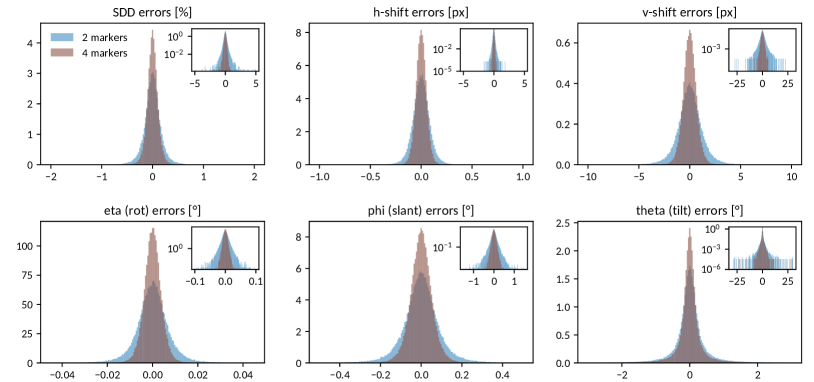
Figure 5: Normalized histograms (probability densities) of the reconstruction errors found for projection geometries reconstructed from noisy (1/2 pixel standard deviation) projections of circular trajectories. Actual projection geometries and trajectories are generated randomly. The reconstructions have been performed using either four (purple) or only two (blue) of the projected trajectories. The inset graphs visualize the tails of the respective distributions using a logarithmic scale. Table 1 summarizes the error ranges for a 98% confidence interval.

	source–detector	horizontal	vertical	detector	detector	detector
	distance	detector shift	detector shift	slant ($\varphi$)	rotation ($\eta$)	tilt ($\theta$)
4 markers	$\pm 0.3\%$	$\pm 0.13$px	$\pm 1.7$px	$\pm 0.14\text{°}$	$\pm 0.01\text{°}$	$\pm 1.6\text{°}$
2 markers	$\pm 0.5\%$	$\pm 0.22$px	$\pm 3.6$px	$\pm 0.27\text{°}$	$\pm 0.02\text{°}$	$\pm 2.3\text{°}$

Table 1: Geometry reconstruction errors within a 98% confidence interval for reconstructions based on two and four projected marker trajectories respectively.

                           

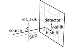
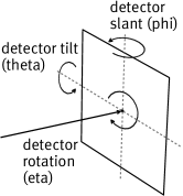
Figure 6: Sketches depicting the employed geometry parametrization. The source–detector distance SDD is measured parallel to the source position vector $\vec{s}$, horizontal ($h$) and vectical ($v$) detector shifts are measured in units of the row and column vectors $\vec{H}$ and $\vec{V}$. The detector orientation is characterized by the angles $\varphi$ and $\theta$ describing the orientation of its normal with respect to the source orientation $\vec{s}$ as well as the angle $\varphi$ describing the in-plane rotation of the detector about its normal.

Calibration was performed based on the solution strategy for Eqs. 31–37 derived in Section 7.2. More specifically, each projected trajectory is first reduced to its sinusoid parameters by means of Algorithm 2. Based on these observables, a self consistent solution for markers and projection matrix is found by means of Algorithm 1. The projective ambiguities are resolved by means of Eq. 38, 62 and 87 constraining the detector rows and columns to be orthogonal and the pixel aspect ratio to be 1. The resulting projection matrix is transformed into real space geometry vectors describing relative source and detector position as well as row and column orientation by means of Eq. 84 and the known detector pixel pitch. In order to compare this result to the original (randomly generated) imaging geometry, the reconstructed geometry is finally rotated and shifted about and along the $z$ axis respectively such that the source comes to line on the $y$ axis.

Figure 5 shows the distribution of errors found for $10^{6}$ random realizations of the just described experiment. Table 1 summarizes the error ranges corresponding to a 98% confidence interval, i.e. in 98% of the cases, the true values will lie within the listed intervals about the reconstructed values. Figure 6 sketches the chosen geometry parametrization.

Particularly the distribution of errors on the detector tilt towards the rotational axis exhibits long tails including rare (as seldom as one in a million) yet extreme deviations (up to 25°) from the true value. As the detector tilt is part of the projective ambiguity in the solution of Equations 29–37 as detailed in Section 2.2, it has to be inferred by enforcing a known detector pixel geometry. As the latter is implicitly assumed to be unaffected by noise, any actual noise will translate onto the remaining parameters of the imaging geometry, causing large uncertainties on the inferred tilt. Further, as the determined homography inversely applies to the reconstructed sample, errors on the detector tilt will come along with errors on the $z$ scale and consequently on the aspect ratio of the reconstructed samples.

4 Discussion

An auto-calibration method for cone beam tomography systems has been derived from the projection matrix formulation of the perspective projection of rotating fiducial markers. The representation in cylinder coordinates directly reveals both a fractions-of-sinusoids model describing the observable projections as well as linear relations of this model’s parameters to both the unknown projection matrix and the parameters of the circular marker trajectories. (In the case of known trajectory parameters, the system of equations could at this point be directly solved for the unknown projection matrix analog to other projection matrix calibration methods based on known objects [RougeeTrousset1993, StrobelWiesent2003, XLiBLiu2010].) An iterative scheme is proposed that alternatingly solves the linear system of equations with respect to the projection matrix and the trajectories until a self consistent solution is obtained, starting with initial approximations for the trajectory parameters. A simple weighting heuristic accounts for the adequate consideration of redundant equations. The ambiguities in the self consistent solution are formalized to a sparse homography matrix, which is then constrained based on knowledge of the detector pixel geometry. Finally, a transformation of projection matrices into real space vectors describing source and detector position as well as detector row and column orientations is given. Other geometry descriptions can be derived from either the projection matrices or the real space vectors using common techniques that have not been further detailed here.

The forward model reveals that the projected circular trajectories are completely described by a total of 8 parameters (which can be identified with those that were previously also used by Smekal et al. [Smekal2004]). In contrast to the ellipse description of projected circles (generally using 5 parameters) that has been used by many authors [Noo2000, Cho2005, StrubelNoo2005, KYangBoone2006, JohnstonBadea2008, RobertMainprize2009, DWuYXiao2011, GrossSchwanecke2012, XuTsui2013], not only the shape, but also the projection angle ($\phi$) dependence is captured correctly in this description. This assumably is the underlying reason why degeneracy of ellipses, which is a major issue for the respective methods based on ellipse paramters, is not a particularly special case in this representation – all 8 parameters are still defined also in the case of an edge-on projection within the plane of rotation of a circular orbit. The forward model itself almost directly exposes the solution to the calibration problem in form of the system of equations relating the sinusoid parameters to the contained system parameters. The employed forward model is further clearly separated into orthographic projections (numerators) and perspective scaling (denominator), allowing for direct interpretations of the parameters. The denominator or perspective scaling component is associated with the third row of the projection matrix (cf. Eqs. 20–26), which in turn describes, as is explicitly shown in Section 2.3.2, the detector normal and focal distance. This clearly highlights that the ability to determine the orientation of the detector normal (i.e., to determine detector slant and tilt) without knowledge of the sample dimensions is ultimately founded in the specific perspective scaling effects associated with the detector orientation. Conversely, this ability becomes restricted in the case of ambiguous scaling effects: in the case of zero detector slant (i.e., the rotational axis intersects the orthogonal connecting line between detector and source), scaling effects due to a potentially tilted detector become indiscernible from an actually distorted sample, and, as has been reported previously by several authors [Rizo1994, Beque2003, WangTsui2007, SawallKachelriess2012], additional knowledge or assumptions will thus be required (usually, the assumption of zero detector tilt will be adequate given its typically small effect [Noo2000, Smekal2004, KYangBoone2006]). In the present method, this ambiguity manifests itself in a degenerate minimum of the objective function used to determine the homography parameters as discussed in Section 2.2.

Regarding the positioning or selection of fiducial markers within the field of view, although no explicit analyses have been shown, several general arguments can be made. First of all, markers obviously must not be located on the rotational axis, i.e., the radius of its circular trajectory must not be zero. The larger the radius relative to the detector grid, the smaller the relative errors in the determination of the projected positions. Larger radii further imply larger covered cone angles and thus more pronounced perspective scaling effects, which have been identified to be essential to auto-calibration from unknown samples. Analogously, although edge-on projections are not a fundamental issue here, trajectories further away from the cone center plane will exhibit stronger perspective effects and are therefore expected to be favorable. This is also consistent with the observations by Bequé et al. [Beque2005] in context of their least squares optimization approach. Also, placement of markers only within one half of the cone does not constitute a special case, in contrast to ellipse based methods as introduced by Noo et al. [Noo2000]. In order to account for the original assumption of the present work that markers are apriori unknown, the presented simulation study intentionally addresses a wide range of imaginable marker placements and projection geometries, without explicitly investigating potentially favorable configurations.

One reason for the simplicity of the present calibration approach lies in the additional degree of freedom of oblique detector grids that is implicit in the projection matrix formalism. The relation between detector tilt and detector grid geometry through the homography parameters $\gamma$ and $\delta$ (cf. Sections 2.2 and 7.1) on the one hand allows to shift the determination of tilt into a downstream postprocessing procedure, and on the other hand provides another view on the previously reported imprecision immanent to the determination of detector tilt [Smekal2004, GrossSchwanecke2012], which could also be observed in the present results. The imprecision in the determination of tilt is in fact an imprecision in the determination of the correct homography transformation (affecting both the projection matrix and the object coordinate system) based on constraints on the detector geometry instead of constraints on the sample geometry. As even considerable tilts in the range of degrees translate to rather moderate amounts of detector non-orthogonality, the noise susceptibility for the converse inference of tilt by means of constraining detector shear is very high. In particular the long tails of the error distribution found in the present simulations (cf. Fig. 5 and Table 1) evidence a very high uncertainty in the determination of tilt that often ranges within the order of magnitude of its actual value. The plain assumption of zero tilt is thus, as has been concluded by others previously [Smekal2004, GrossSchwanecke2012], often well within the error margin. In contrast to previous work though, which by design also constrained the detector geometry, consistency won’t be affected here, as actual effects due to tilt will still be accounted for by means of an artificially oblique detector geometry.

The remaining homography parameters regarding the choice of origin and scale of the coordinate system have not been explicitly treated. They are straight-forwardly chosen based on the real space geometry description extracted from the reconstructed projection matrix (cf. Section 2.3.2) in order to e.g. align the source position or the detector normal with the $x$-$z$ or $y$-$z$ plane and scale and shift source and detector within the available degrees of freedom such that a user defined tomographic reconstruction field of view optimally fits the projection cone.

5 Conclusion

A projection matrix based approach to the auto-calibration of the projection geometry of cone beam computed tomography systems from apriori unknown fiducial markers moving along circular trajectories has been proposed. In contrast to previous literature, the problem of calibration has been decoupled from the particular choice of real space geometry parametrization, allowing for a very simple representation of the core problem without having to fall back to generic optimization approaches. The link to classic, more intuitive geometry representations is provided by means of explicit conversion formulas of projection matrices to real space position and orientation vectors. The formulation of ambiguities in terms of homography transformations further reveals the relation to methods based on known samples, which essentially differ in the particular prior knowledge used to constrain the solution space. The proposed scheme for the self consistent solution of the derived system of equations both with respect to the unknown projection and sample parameters has been tested on a large variety of simulated noisy projection data in order to assess the average precision independent of the particular instances of marker placement, noise and geometric configuration of the projection system. A high degree of versatility is achieved by avoiding the necessity of prior estimates on the system or sample parameters which is commonly required for methods based on the optimization of a cost function. Last but not least, the present formulation provides another, hopefully more intuitive view, on the auto-calibration problem, allowing further insights into the fundamental working principle and limitations of auto-calibration of cone beam computed tomography systems from unknown samples.

6 Acknowledgments

The author thanks Prof. Dr. Randolf Hanke and Dr. habil. Simon Zabler for facilitating the present work. Dr. Christian Fella, Dr. Kilian Dremel and Dominik Müller are acknowledged for providing experimental data used to test the presented methods during the stages of development. Funding is acknowledged from the Bavarian State Ministry of Economic Affairs, Infrastructure, Transport and Technology which supported the project group ”Nano-CT Systems for Material Characterization”, the European Horizon 2020 project no. 814485 (LEE-BED), and the German Federal Ministry of Education and Research grant 05E19AN1 supporting the BM18 beamline at the European Synchrotron Radiation Facility ESRF.

7 Appendix

7.1 Projective ambiguities

7.1.1 Detector pixel aspect ratio

When considering the relations $r_{i}^{\prime}P_{m\mathrm{a}}=a_{im}$ (Eqs. 29–31) and assuming some consistent solutions for $r_{i}^{\prime}$ and $P_{m\mathrm{a}}$ have already been found, it is easy to see that these solutions may be scaled by an arbitrary factor $\alpha\neq 0$:

$$r_{i}^{\prime}P_{m\mathrm{a}}=r_{i}^{\prime}\frac{\alpha}{\alpha}P_{m\mathrm{a}}=(\alpha r_{i}^{\prime})(\frac{1}{\alpha}P_{m\mathrm{a}})=\tilde{r}_{i}^{\prime}\tilde{P}_{m\mathrm{a}}=a_{im}\quad.$$

The same is true for $z_{i}^{\prime}$ and $P_{m3}$ (Eqs. 32–34):

$$z_{i}^{\prime}P_{m3}=z_{i}^{\prime}\frac{\beta}{\beta}P_{m3}=(\beta z_{i}^{\prime})(\frac{1}{\beta}P_{m3})=\tilde{z}_{i}^{\prime}\tilde{P}_{m3}=o_{im}$$

with an independent scaling parameter $\beta\neq 0$. While the freedom to choose an arbitrary overall scale corresponds to the unknown absolute size of the imaged phantom, the freedom to choose independent scales for the $x$-$y$ and the $z$ dimensions or equivalently for $r_{i}^{\prime}$ and $z_{i}^{\prime}$ or $P_{m\mathrm{a}}$ and $P_{m3}$ corresponds to the disregarded pixel pitches of the detector, i.e. the calibration equations can equally be satisfied by a detector with asymmetric pixels and a correspondingly squeezed or stretched object.

Conversely, this ambiguity corresponding to the homography parameter $\delta$ can be resolved by choosing the relative scale $\alpha/\beta=\delta_{\varepsilon}$ such that the detector encoded in $\boldsymbol{P}$ actually features the correct pixel aspect ratio (denoted by $\varepsilon$) for the given hardware. As derived in Section 2.3.2, the vector products $(P_{11},P_{12},P_{13})\times(P_{31},P_{32},P_{33})$ and $(P_{21},P_{22},P_{23})\times(P_{31},P_{32},P_{33})$ are proportional to the detector row and column vectors $\vec{H}$ and $\vec{V}$ (Fig. 2, Eq. 85). Given a known pixel aspect ratio $\varepsilon\overset{!}{=}\bigl{\|}\vec{H}\bigr{\|}/\bigl{\|}\vec{V}\bigr{\|}$, $\delta_{\varepsilon}$ may therefore be defined as the solution to

$$\varepsilon\bigl{\|}\vec{V}(\delta_{\varepsilon})\bigr{\|} \overset{!}{=}\bigl{\|}\vec{H}(\delta_{\varepsilon})\bigr{\|}$$

$$\varepsilon\left\|(P_{11},P_{12},\delta_{\varepsilon}P_{13})\times(P_{31},P_{32},\delta_{\varepsilon}P_{33})\right\| =\left\|(P_{21},P_{22},\delta_{\varepsilon}P_{23})\times(P_{31},P_{32},\delta_{\varepsilon}P_{33})\right\|\quad,$$

i.e.

$$\delta_{\epsilon} =\sqrt{\frac{(P_{21}P_{32}-P_{22}P_{31})^{2}-\varepsilon^{2}(P_{11}P_{32}-P_{12}P_{31})^{2}}{\begin{multlined}\varepsilon^{2}(P_{12}P_{33}-P_{13}P_{32})^{2}+\varepsilon^{2}(P_{13}P_{31}-P_{11}P_{33})^{2}\\ -(P_{22}P_{33}-P_{23}P_{32})^{2}-(P_{23}P_{31}-P_{21}P_{33})^{2}\end{multlined}\varepsilon^{2}(P_{12}P_{33}-P_{13}P_{32})^{2}+\varepsilon^{2}(P_{13}P_{31}-P_{11}P_{33})^{2}\\ -(P_{22}P_{33}-P_{23}P_{32})^{2}-(P_{23}P_{31}-P_{21}P_{33})^{2}}}$$ (86)

$$=\sqrt{\frac{H_{z}^{2}-\varepsilon^{2}V_{z}^{2}}{\varepsilon^{2}(V_{x}^{2}+V_{y}^{2})-(H_{x}^{2}+H_{y}^{2})}}\quad,$$

where the $H_{x},H_{y},H_{z}$ and $V_{x},V_{y},V_{z}$ components refer here to those prior to the correction by the derived scaling factor $\delta_{\varepsilon}$ to be applied to $P_{m3}$ (and inversely to $z_{i}^{\prime}$) in order to make $\boldsymbol{P}$ (and in consequence also the corresponding euclidean vectors $\vec{s}$, $\vec{d}$, $\vec{H}$ and $\vec{V}$) consistent with the known detector pixel aspect ratio $\varepsilon$ (which commonly will be $\varepsilon=1$).

7.1.2 Detector tilt and shear

Also the relations $P_{m3}z_{i}^{\prime}+P_{m4}w_{i}=o_{im}$ (Eqs. 32–34) may similarly be satisfied by transformed $\tilde{P}_{m3}$, $\tilde{z}_{i}^{\prime}$ and $\tilde{w}_{i}$, now including also $\gamma$:

$$P_{m3}z_{i}^{\prime}+P_{m4}w_{i}=\delta(P_{m3}-\gamma P_{m4})(\frac{1}{\delta}z_{i}^{\prime})+P_{m4}(w_{i}+\gamma z_{i}^{\prime})=\tilde{P}_{m3}\tilde{z}_{i}^{\prime}+P_{m4}\tilde{w}_{i}=o_{im}\quad.$$

The role of $\delta$ has just been discussed, wherefore $\delta$ will be assumed to equal $1$ for now. The parameter $\gamma$ relating $w_{i}$ and $P_{m3}$ will in effect control the detector tilt and shear as will be explained in the following.

Equation 34 ($P_{33}z_{i}^{\prime}+P_{34}w_{i}=o_{i\mathrm{w}}=1$) concerning the mean $o_{i\mathrm{w}}=1$ of the projection equations’ denominators (cf. Eqs. 27 and 28) reveals that for $w_{i}=\mathrm{const.}$, $P_{33}$ must equal $0$. Vice versa, $w_{i}$ varying among several imaged trajectories $i$ (i.e. being $z_{i}^{\prime}$-dependent) implies $P_{33}\neq 0$. Given $\tilde{w}_{i}=w_{i}+\gamma z_{i}^{\prime}$ and $\tilde{P}_{33}=P_{33}-\gamma P_{34}$, it can therefore be concluded that both the relevance of the homogeneous coordinates’ scaling components $w_{i}$ and the role of the homography parameter $\gamma$ are directly related to the $P_{33}$ component of the projection matrix. Section 2.3.2 shows that the vector $(P_{31},P_{32},P_{33})$ in the last row of $\boldsymbol{P}$ corresponds to the cross product $\vec{H}\times\vec{V}$ of the detector row and column orientations and is therefore normal to the detector plane. The $z$ component $P_{33}$ is thus directly related to the detector tilt towards the rotational axis, which was defined to coincide with the $z$-axis. In consequence, $\gamma$ controls the detector tilt encoded in $\tilde{\boldsymbol{P}}$. As changes to $P_{m3}$ have more general implications on the cross products of $(\vec{d}-\vec{s})$, $\vec{H}$ and $\vec{V}$ encoded in the first three columns of $\boldsymbol{P}$, $\gamma$ will also influence the angle between $\vec{H}$ and $\vec{V}$. As this is commonly a known property of the detector (typically, $\vec{H}\cdot\vec{V}=0$), it can be used to constrain $\gamma$ and consequently to determine the detector tilt towards the $z$-axis. As $\gamma$ will as well affect the norms of $\vec{H}$ and $\vec{V}$, i.e. the pixel aspect ratio, $\gamma$ usually needs to be determined simultaneously with $\delta$ using a suiting objective function constraining both the pixel aspect ratio and orthogonality:

$$\gamma,\delta_{\varepsilon}=\underset{\gamma,\delta}{\mathrm{argmin}}\left(\left(\frac{\Bigl{\|}\vec{H}(\gamma,\delta)\Bigr{\|}-\varepsilon\Bigl{\|}\vec{V}(\gamma,\delta)\Bigr{\|}}{\Bigl{\|}\vec{H}(\gamma,\delta)\Bigr{\|}+\varepsilon\Bigl{\|}\vec{V}(\gamma,\delta)\Bigr{\|}}\right)^{2}+\left(\frac{\vec{H}(\gamma,\delta)\cdot\vec{V}(\gamma,\delta)}{\Bigl{\|}\vec{H}(\gamma,\delta)\Bigr{\|}\,\Bigl{\|}\vec{V}(\gamma,\delta)\Bigr{\|}}\right)^{2}\right)$$ (87)

with $\varepsilon$ denoting the pixel aspect ratio and assuming that the detector rows and columns are expected to be orthogonal. In case of actually non-orthogonal detectors such as hexagonal pixel arrangements, the objective function may be adjusted accordingly to favor the respective expected shear angle.

The detector tilt has been identified by many authors to have the smallest influence on the observable projections and therefore can, in the presence of noise, only be determined with very little precision. In particular in the context of calibration based on unknown phantoms, the detector is therefore often fixed to be parallel to the rotational axis. For the method presented here, this is equivalent to fixing $w_{i}$ to $1$ and consequently $P_{33}$ to $0$, either by choice of $\gamma$ or simply by directly choosing the $w_{i}$-related relaxation parameter $\lambda_{w}=0$ within the iterative reconstruction of $\boldsymbol{P}$ (cf. Section 7.2). Actual detector tilts will then manifest themselves in a slight amount of artificial shear (slightly non-orthogonal detector rows and columns) in the determined projection geometry. As this corresponds to a valid projective homography, resulting tomographic reconstructions using so constrained geometries will be transformed by the corresponding inverse homography. In contrast to the case of both constrained tilt and pixel geometry, actual artifacts due to geometric inconsistencies are avoided.

In accordance with the findings by Smekal et al. [Smekal2004], the tilt cannot be uniquely determined when the detector is not slanted about the rotational axis. This remaining ambiguity manifests itself in a non-unique minimum of the objective function in Eq. 87 in the case of zero detector slant.

7.2 Iterative projection matrix reconstruction

$\negmedspace\negmedspace\left.\begin{array}[]{lll}a_{i\mathrm{h}}&\phi_{i0\mathrm{h}}&o_{i\mathrm{h}}\\ a_{i\mathrm{v}}&\phi_{i0\mathrm{v}}&o_{i\mathrm{v}}\\ a_{i\mathrm{w}}&\phi_{i0\mathrm{w}}&o_{i\mathrm{w}}\end{array}\right\}\leftarrow\;\mathrm{Algorithm}\leavevmode\nobreak\ \ref{alg:pmat-recon-sinusoids}\leavevmode\nobreak\ (h_{i}(\phi),v_{i}(\phi))\;\forall\,i$ $\triangleright$ $\begin{array}[]{l}\text{Sinusoid parameters extracted}\\ \text{from projection data }\end{array}\negmedspace\negmedspace\negmedspace$

$r_{i}^{\prime(0)}\leftarrow a_{i\mathrm{h}}$ $\triangleright$ initialize radii with horizontal trajectory amplitudes

$z_{i}^{\prime(0)}\leftarrow o_{i\mathrm{v}}$ $\triangleright$ initialize $z$-coordinates with vertical means

$P_{m\mathrm{a}}^{(0)}\leftarrow\vphantom{\smash[b]{\Bigg{(}}}\frac{\sum_{i}r_{i}^{\prime(0)}a_{im}}{\sum_{i}r_{i}^{\prime(0)\,2}}$$\triangleright$ initialize with (weighted) mean amplitudes

$P_{m3}^{(0)}\leftarrow\vphantom{\Bigg{(}}\frac{\sum_{i}(z_{i}^{\prime(0)}-\overline{z^{\prime}}^{(0)})(o_{im}-\overline{o}_{m})}{\sum_{i}(z_{i}^{\prime(0)}-\overline{z^{\prime}}^{(0)})^{2}}$$\triangleright$ $P_{m3}^{(0)},P_{m4}^{(0)}=\underset{P_{m3},P_{m4}}{\mathrm{argmin}}\left(P_{m3}\,z_{i}^{\prime(0)}+P_{m4}-o_{im}\right)$

$P_{m4}^{(0)}\leftarrow\vphantom{\smash[t]{\Bigg{(}}}\overline{o}_{m}-P_{m3}^{(0)}\,\overline{z^{\prime}}^{(0)}$$\triangleright$ $\mathrlap{\text{with}\quad\overline{z^{\prime}}^{(0)}=\frac{1}{N}\sum_{i}z_{i}^{\prime(0)};\quad\overline{o}_{m}=\frac{1}{N}\sum_{i}o_{im}}\hphantom{P_{m3}^{(0)},P_{m4}^{(0)}=\underset{P_{m3},P_{m4}}{\mathrm{argmin}}\left(P_{m3}\,z_{i}^{\prime(0)}+P_{m4}-o_{im}\right)}$

for $k=0\,..\,N_{\mathrm{iter}}-1$ do with $\lambda\in\;]0;1]$$\triangleright$ iteratively enforce Eqs. 29–34

     $r_{i}^{\prime(k+1)}\leftarrow\vphantom{\Bigg{(}}(1-\lambda)r_{i}^{\prime(k)}+\lambda\,\frac{\sum_{m}P_{m\mathrm{a}}^{(k)}a_{im}}{\sum_{m}P_{m\mathrm{a}}^{(k)\,2}}$

     $z_{i}^{\prime(k+1)}\leftarrow(1-\lambda)z_{i}^{\prime(k)}+\lambda\frac{\sum_{m}P_{m3}^{(k)}(o_{im}-P_{m4}^{(k)})}{\sum_{m}P_{m3}^{(k)\,2}}$

     $P_{m\mathrm{a}}^{(k+1)}\leftarrow\vphantom{\Bigg{(}}(1-\lambda)P_{m\mathrm{a}}^{(k)}+\lambda\,\frac{\sum_{i}r_{i}^{\prime(k)}a_{im}}{\sum_{i}r_{i}^{\prime(k)\,2}}$

     $P_{m3}^{(k+1)}\leftarrow(1-\lambda)P_{m3}^{(k)}+\lambda\,\frac{\sum_{i}(z_{i}^{\prime(k)}-\overline{z^{\prime}}^{(k)})(o_{im}-\overline{o}_{m})}{\sum_{i}(z_{i}^{\prime(k)}-\overline{z^{\prime}}^{(k)})^{2}}$$\triangleright$ $\underset{P_{m3},P_{m4}}{\mathrm{argmin}}\left(P_{m3}\,z_{i}^{\prime(k)}+P_{m4}-o_{im}\right)$

     $P_{m4}^{(k+1)}\leftarrow\vphantom{\Bigg{(}}(1-\lambda)P_{m4}^{(k)}+\lambda\,\big{(}\overline{o}_{m}-P_{m3}^{(k)}\,\overline{z^{\prime}}^{(k)}\big{)}$$\triangleright$ $\mathrlap{\overline{z^{\prime}}^{(k)}\!\!=\!\frac{1}{N}\!\sum_{i}z_{i}^{\prime(k)};\;\overline{o}_{m}\!=\!\frac{1}{N}\!\sum_{i}o_{im}}\hphantom{\underset{P_{m3},P_{m4}}{\mathrm{argmin}}\left(P_{m3}\,z_{i}^{\prime(k)}+P_{m4}-o_{im}\right)}$

end for

$\phi_{\mathrm{h}}\leftarrow 0$

$\phi_{\mathrm{v}}\leftarrow\arg\left(\sum_{i}(e^{\boldsymbol{i}(\phi_{i0\mathrm{v}}-\phi_{i0\mathrm{h}})}a_{i\mathrm{v}}^{2}a_{i\mathrm{h}}^{2})\right)$

$\phi_{\mathrm{w}}\leftarrow\arg\left(\sum_{i}(e^{\boldsymbol{i}(\phi_{i0\mathrm{w}}-\phi_{i0\mathrm{h}})}a_{i\mathrm{w}}^{2}a_{i\mathrm{h}}^{2})\right)$

$\phi_{i0}\leftarrow\arg\left(\sum_{m}(e^{\boldsymbol{i}(\phi_{i0m}-\phi_{m})}a_{im}^{2})\right)$

$\boldsymbol{P}\leftarrow\left[\begin{array}[]{cccc}-P_{1\mathrm{a}}\sin(\phi_{\mathrm{h}})&P_{1\mathrm{a}}\cos(\phi_{\mathrm{h}})&P_{13}&P_{14}\\ -P_{2\mathrm{a}}\sin(\phi_{\mathrm{v}})&P_{2\mathrm{a}}\cos(\phi_{\mathrm{v}})&P_{23}&P_{14}\\ -P_{3\mathrm{a}}\sin(\phi_{\mathrm{w}})&P_{3\mathrm{a}}\cos(\phi_{\mathrm{w}})&P_{33}&P_{14}\end{array}\right];\quad\quad\boldsymbol{x}_{i}\leftarrow\left[\begin{array}[]{c}\hphantom{-}r^{\prime}_{i}\cos(\phi_{i0})\\ -r^{\prime}_{i}\sin(\phi_{i0})\\ z^{\prime}_{i}\\ 1\end{array}\right]$

$\boldsymbol{P}\leftarrow\boldsymbol{P}\boldsymbol{H}^{-1};\quad\boldsymbol{x}_{i}\leftarrow\boldsymbol{H}\boldsymbol{x}_{i}$ $\triangleright$ resolve projective ambiguities with additional contraints,

cf. Sections 2.2 and 7.1, especially Eqs. 38, 62, 86, 87

$\vec{s},\vec{d},\vec{H},\vec{V}\leftarrow\text{Eq.\leavevmode\nobreak\ \ref{eq:pmat-to-constrainedgeom}}$ $\triangleright$ Transform to real space representation and potentially apply

further application-specific coordinate transformations

Algorithm 1 Self-consistent reconstruction of projection matrix and marker coordinates from projections of circular marker trajectories (solving Eqs. 29–37). The homogeneous scaling components $w_{i}$ are, without loss of generality, constrained to $1$ (thereby constraining the detector tilt angle towards the rotational axis to $\theta=0$). Differing values of tilt and scaling of the marker trajectories can be recovered subsequently based on projective homographies as outlined in Sections 2.2 and 7.1.

$\mathrlap{\phi_{j}}\hphantom{h_{\mathrm{cc}_{2}}}=2\pi/N\,j$

$\mathrlap{h_{j}}\hphantom{h_{\mathrm{cc}_{2}}}=h(\phi_{j})$

$\mathrlap{v_{j}}\hphantom{h_{\mathrm{cc}_{2}}}=v(\phi_{j})$

$\mathrlap{\overline{h}}\hphantom{h_{\mathrm{cc}_{2}}}=\frac{1}{N}\sum_{j=0}^{N-1}h_{j}$

$\mathrlap{h_{\mathrm{s}}}\hphantom{h_{\mathrm{cc}_{2}}}=\frac{1}{N}\sum_{j=0}^{N-1}h_{j}\sin(\phi_{j})$

$\mathrlap{h_{\mathrm{c}}}\hphantom{h_{\mathrm{cc}_{2}}}=\frac{1}{N}\sum_{j=0}^{N-1}h_{j}\cos(\phi_{j})$

$\mathrlap{h_{\mathrm{ss}}}\hphantom{h_{\mathrm{cc}_{2}}}=\frac{1}{N}\sum_{j=0}^{N-1}h_{j}\sin^{2}(\phi_{j})$

$\mathrlap{h_{\mathrm{sc}}}\hphantom{h_{\mathrm{cc}_{2}}}=\frac{1}{N}\sum_{j=0}^{N-1}h_{j}\sin(\phi_{j})\cos(\phi_{j})$

$\mathrlap{h_{\mathrm{cc}}}\hphantom{h_{\mathrm{cc}_{2}}}=\frac{1}{N}\sum_{j=0}^{N-1}h_{j}\cos^{2}(\phi_{j})$

$\mathrlap{h_{\mathrm{s_{2}}}}\hphantom{h_{\mathrm{cc}_{2}}}=\frac{1}{N}\sum_{j=0}^{N-1}h_{j}\sin(2\phi_{j})$

$\mathrlap{h_{\mathrm{c_{2}}}}\hphantom{h_{\mathrm{cc}_{2}}}=\frac{1}{N}\sum_{j=0}^{N-1}h_{j}\cos(2\phi_{j})$

$\mathrlap{h_{\mathrm{s}_{2}\mathrm{s}}}\hphantom{h_{\mathrm{cc}_{2}}}=\frac{1}{N}\sum_{j=0}^{N-1}h_{j}\sin(2\phi_{j})\sin(\phi_{j})$

$\mathrlap{h_{\mathrm{s}_{2}\mathrm{c}}}\hphantom{h_{\mathrm{cc}_{2}}}=\frac{1}{N}\sum_{j=0}^{N-1}h_{j}\sin(2\phi_{j})\cos(\phi_{j})$

$\mathrlap{h_{\mathrm{sc}_{2}}}\hphantom{h_{\mathrm{cc}_{2}}}=\frac{1}{N}\sum_{j=0}^{N-1}h_{j}\sin(\phi_{j})\cos(2\phi_{j})$

$\mathrlap{h_{\mathrm{cc}_{2}}}\hphantom{h_{\mathrm{cc}_{2}}}=\frac{1}{N}\sum_{j=0}^{N-1}h_{j}\cos(\phi_{j})\cos(2\phi_{j})$

$\mathrlap{\overline{v}}\hphantom{v_{\mathrm{cc}_{2}}}=\frac{1}{N}\sum_{j=0}^{N-1}v_{j}$

$\mathrlap{v_{\mathrm{s}}}\hphantom{v_{\mathrm{cc}_{2}}}=\frac{1}{N}\sum_{j=0}^{N-1}v_{j}\sin(\phi_{j})$

$\mathrlap{v_{\mathrm{c}}}\hphantom{v_{\mathrm{cc}_{2}}}=\frac{1}{N}\sum_{j=0}^{N-1}v_{j}\cos(\phi_{j})$

$\mathrlap{v_{\mathrm{ss}}}\hphantom{v_{\mathrm{cc}_{2}}}=\frac{1}{N}\sum_{j=0}^{N-1}v_{j}\sin^{2}(\phi_{j})$

$\mathrlap{v_{\mathrm{sc}}}\hphantom{v_{\mathrm{cc}_{2}}}=\frac{1}{N}\sum_{j=0}^{N-1}v_{j}\sin(\phi_{j})\cos(\phi_{j})$

$\mathrlap{v_{\mathrm{cc}}}\hphantom{v_{\mathrm{cc}_{2}}}=\frac{1}{N}\sum_{j=0}^{N-1}v_{j}\cos^{2}(\phi_{j})$

$\mathrlap{v_{\mathrm{s_{2}}}}\hphantom{v_{\mathrm{cc}_{2}}}=\frac{1}{N}\sum_{j=0}^{N-1}v_{j}\sin(2\phi_{j})$

$\mathrlap{v_{\mathrm{c_{2}}}}\hphantom{v_{\mathrm{cc}_{2}}}=\frac{1}{N}\sum_{j=0}^{N-1}v_{j}\cos(2\phi_{j})$

$\mathrlap{v_{\mathrm{s}_{2}\mathrm{s}}}\hphantom{v_{\mathrm{cc}_{2}}}=\frac{1}{N}\sum_{j=0}^{N-1}v_{j}\sin(2\phi_{j})\sin(\phi_{j})$

$\mathrlap{v_{\mathrm{s}_{2}\mathrm{c}}}\hphantom{v_{\mathrm{cc}_{2}}}=\frac{1}{N}\sum_{j=0}^{N-1}v_{j}\sin(2\phi_{j})\cos(\phi_{j})$

$\mathrlap{v_{\mathrm{sc}_{2}}}\hphantom{v_{\mathrm{cc}_{2}}}=\frac{1}{N}\sum_{j=0}^{N-1}v_{j}\sin(\phi_{j})\cos(2\phi_{j})$

$\mathrlap{v_{\mathrm{cc}_{2}}}\hphantom{v_{\mathrm{cc}_{2}}}=\frac{1}{N}\sum_{j=0}^{N-1}v_{j}\cos(\phi_{j})\cos(2\phi_{j})$

$\mathrlap{s_{\mathrm{w}}}\hphantom{h_{\mathrm{cc}_{2}}}=\frac{(h_{\mathrm{s}_{2}\mathrm{c}}h_{\mathrm{sc}_{2}}-h_{\mathrm{s}_{2}\mathrm{s}}h_{\mathrm{cc}_{2}})(h_{\mathrm{cc}_{2}}h_{\mathrm{s_{2}}}-h_{\mathrm{s}_{2}\mathrm{c}}h_{\mathrm{c_{2}}})+(v_{\mathrm{s}_{2}\mathrm{c}}v_{\mathrm{sc}_{2}}-v_{\mathrm{s}_{2}\mathrm{s}}v_{\mathrm{cc}_{2}})(v_{\mathrm{cc}_{2}}v_{\mathrm{s_{2}}}-v_{\mathrm{s}_{2}\mathrm{c}}v_{\mathrm{c_{2}}})}{(h_{\mathrm{s}_{2}\mathrm{c}}h_{\mathrm{sc}_{2}}-h_{\mathrm{s}_{2}\mathrm{s}}h_{\mathrm{cc}_{2}})^{2}+(v_{\mathrm{s}_{2}\mathrm{c}}v_{\mathrm{sc}_{2}}-v_{\mathrm{s}_{2}\mathrm{s}}v_{\mathrm{cc}_{2}})^{2}}$

$\mathrlap{c_{\mathrm{w}}}\hphantom{h_{\mathrm{cc}_{2}}}=\frac{(h_{\mathrm{s}_{2}\mathrm{c}}h_{\mathrm{sc}_{2}}-h_{\mathrm{s}_{2}\mathrm{s}}h_{\mathrm{cc}_{2}})(h_{\mathrm{s}_{2}\mathrm{s}}h_{\mathrm{c_{2}}}-h_{\mathrm{sc}_{2}}h_{\mathrm{s_{2}}})+(v_{\mathrm{s}_{2}\mathrm{c}}v_{\mathrm{sc}_{2}}-v_{\mathrm{s}_{2}\mathrm{s}}v_{\mathrm{cc}_{2}})(v_{\mathrm{s}_{2}\mathrm{s}}v_{\mathrm{c_{2}}}-v_{\mathrm{sc}_{2}}v_{\mathrm{s_{2}}})}{(h_{\mathrm{s}_{2}\mathrm{c}}h_{\mathrm{sc}_{2}}-h_{\mathrm{s}_{2}\mathrm{s}}h_{\mathrm{cc}_{2}})^{2}+(v_{\mathrm{s}_{2}\mathrm{c}}v_{\mathrm{sc}_{2}}-v_{\mathrm{s}_{2}\mathrm{s}}v_{\mathrm{cc}_{2}})^{2}}$

$\mathrlap{s_{\mathrm{h}}}\hphantom{h_{\mathrm{cc}_{2}}}=2(\mathrlap{s_{\mathrm{w}}h_{\mathrm{ss}}}\hphantom{s_{\mathrm{w}}h_{\mathrm{sc}}}+\mathrlap{c_{\mathrm{w}}h_{\mathrm{sc}}}\hphantom{c_{\mathrm{w}}h_{\mathrm{cc}}}+h_{\mathrm{s}})$

$\mathrlap{c_{\mathrm{h}}}\hphantom{h_{\mathrm{cc}_{2}}}=2(s_{\mathrm{w}}h_{\mathrm{sc}}+c_{\mathrm{w}}h_{\mathrm{cc}}+u_{\mathrm{c}})$

$\mathrlap{o_{\mathrm{h}}}\hphantom{h_{\mathrm{cc}_{2}}}=\hphantom{2(}\mathrlap{s_{\mathrm{w}}h_{\mathrm{s}}}\hphantom{s_{\mathrm{w}}h_{\mathrm{sc}}}+\mathrlap{c_{\mathrm{w}}h_{\mathrm{c}}}\hphantom{c_{\mathrm{w}}h_{\mathrm{cc}}}+\overline{h}$

$\mathrlap{a_{\mathrm{h}}}\hphantom{h_{\mathrm{cc}_{2}}}=\sqrt{s_{\mathrm{h}}^{2}+c_{\mathrm{h}}^{2}}$

$\mathrlap{\phi_{\mathrm{h}0}}\hphantom{h_{\mathrm{cc}_{2}}}=\arctan\!2(-c_{\mathrm{h}},s_{\mathrm{h}})$

$\mathrlap{s_{\mathrm{v}}}\hphantom{v_{\mathrm{cc}_{2}}}=2(\mathrlap{s_{\mathrm{w}}v_{\mathrm{ss}}}\hphantom{s_{\mathrm{w}}v_{\mathrm{sc}}}+\mathrlap{c_{\mathrm{w}}v_{\mathrm{sc}}}\hphantom{c_{\mathrm{w}}v_{\mathrm{cc}}}+v_{\mathrm{s}})$

$\mathrlap{c_{\mathrm{v}}}\hphantom{v_{\mathrm{cc}_{2}}}=2(s_{\mathrm{w}}v_{\mathrm{sc}}+c_{\mathrm{w}}v_{\mathrm{cc}}+v_{\mathrm{c}})$

$\mathrlap{o_{\mathrm{v}}}\hphantom{v_{\mathrm{cc}_{2}}}=\hphantom{2(}\mathrlap{s_{\mathrm{w}}v_{\mathrm{s}}}\hphantom{s_{\mathrm{w}}v_{\mathrm{sc}}}+\mathrlap{c_{\mathrm{w}}v_{\mathrm{c}}}\hphantom{c_{\mathrm{w}}v_{\mathrm{cc}}}+\overline{v}$

$\mathrlap{a_{\mathrm{v}}}\hphantom{v_{\mathrm{cc}_{2}}}=\sqrt{s_{\mathrm{v}}^{2}+c_{\mathrm{v}}^{2}}$

$\mathrlap{\phi_{\mathrm{v}0}}\hphantom{v_{\mathrm{cc}_{2}}}=\arctan\!2(-c_{\mathrm{v}},s_{\mathrm{v}})$

$\mathrlap{o_{\mathrm{w}}}\hphantom{v_{\mathrm{cc}_{2}}}=1$

$\mathrlap{a_{\mathrm{w}}}\hphantom{v_{\mathrm{cc}_{2}}}=\sqrt{s_{\mathrm{w}}^{2}+c_{\mathrm{w}}^{2}}$

$\mathrlap{\phi_{\mathrm{w}0}}\hphantom{v_{\mathrm{cc}_{2}}}=\arctan\!2(-c_{\mathrm{w}},s_{\mathrm{w}})$

Algorithm 2 Extraction of circular trajectories’ sinusoid parameters $a_{i\mathrm{h}}$, $a_{i\mathrm{v}}$, $a_{i\mathrm{w}}$, $\phi_{i0\mathrm{h}}$, $\phi_{i0\mathrm{v}}$, $\phi_{i0\mathrm{w}}$, $o_{i\mathrm{h}}$ and $o_{i\mathrm{v}}$ (cf. Eqs. 27–28) as required for Algorithm 1 from perspective projections $(h_{i}(\phi),v_{i}(\phi))$, assuming an equidistant sampling of the rotation phase $\phi\in[0,2\pi[$. The trajectory index $i$ has been omitted for better readability. A detailed derivation is given in Section 7.3.

Now that the calibration problem has been formalized to the solution of a small system of linear equations, an iterative scheme technique shall be proposed for its self consistent solution. The calibration equations (Eqs. 29–37) may to this end be rearranged for each parameter to be determined, assuming the respective parameters on the right-hand side known (beginning with initial estimates). As there will be multiple analog equations for each parameter relating it to either different rows of the projection matrix or to multiple of the observed projected trajectories, weighted averages will be used to adequately incorporate all available information for each parameter. In order to avoid potential oscillations due to inconsistencies, the iterative updates may be damped by a relaxation factor $\lambda\in[0;1]$ scaling between no update ($\lambda=0$) and no damping ($\lambda=1$).

Without specifying the averaging weights yet, the described scheme results in:

$$w_{i}:\! =1$$

$$r_{i}^{\prime(k+1)} =(1-\lambda)r_{i}^{\prime(k)}+\lambda\left\langle\frac{a_{im}}{P_{m\mathrm{a}}^{(k)}}\right\rangle_{m}$$

$$z_{i}^{\prime(k+1)} =(1-\lambda)z_{i}^{\prime(k)}+\lambda\left\langle\frac{o_{im}-P_{m4}^{(k)}}{P_{m3}^{(k)}}\right\rangle_{m}$$

$$P_{m\mathrm{a}}^{(k+1)} =(1-\lambda)P_{m\mathrm{a}}^{(k)}+\lambda\left\langle\frac{a_{im}}{r_{i}^{\prime(k)}}\right\rangle_{i}$$

$$\begin{array}[]{c}P_{m3}^{(k+1)}\\ P_{m4}^{(k+1)}\end{array}\negmedspace\negmedspace =(1-\lambda)\negmedspace\!\begin{array}[]{c}P_{m3}^{(k)}\\ P_{m4}^{(k)}\end{array}\negmedspace\!+\lambda\>\underset{P_{m3}^{*},P_{m4}^{*}}{\mathrm{argmin}}\bigl{(}P_{m3}^{*}z_{i}^{\prime(k)}+P_{m4}^{*}-o_{im}\bigr{)}^{2}$$

$$\phi_{\mathrm{h}}:\! =0$$

$$\phi_{\mathrm{v}} =\left\langle\phi_{i0\mathrm{v}}-\phi_{i0\mathrm{h}}\right\rangle_{i}$$

$$\phi_{\mathrm{w}} =\left\langle\phi_{i0\mathrm{w}}-\phi_{i0\mathrm{h}}\right\rangle_{i}$$

where $k$ is the iteration index, $\bigl{\langle}\,\cdot\,\bigr{\rangle}_{i}$ and $\bigl{\langle}\,\cdot\,\bigr{\rangle}_{m}$ denote (to be further defined) weighted averages over the marker index $i$ and the projection matrix row index $m$ respectively. For uniformity of the representation, the row related “$\mathrm{h}$”, “$\mathrm{v}$” and “$\mathrm{w}$” indices of the observable sinusoid parameters are equally enumerated by $m$ in the above averages, i.e. $\mathrm{h}\,\widehat{=}\,1,\mathrm{v}\,\widehat{=}\,2,\mathrm{w}\,\widehat{=}\,3$. Based on the discussion given in Section 7.1.2, $w_{i}$ has been chosen $w_{i}=1$ without loss of generality. The parameters $P_{m3},P_{m4}$ are determined by means of linear regression. The phases $\phi_{\mathrm{w}}$ and $\phi_{\mathrm{v}}$ can be evaluated independently as a weighted average over the available observations, whereas $\phi_{\mathrm{h}}$ is, without loss of generality, defined $0$.

Now that the iterative update scheme has been established, actual averaging weights need to be defined. These weights shall respect the varying certainty or error bar associated with the different available equations for each parameter. It will be argued that the denominators occurring in the right-hand-side expressions are reasonable indicators in this respect and may be used as weighting factors, which in addition avoids potential divisions by zero. This can be easily seen on the example of $r_{i}^{\prime}$: the observable amplitudes $a_{im}$ on the right hand side correspond to actual horizontal and vertical ranges covered by the projections observed on a rasterized detector. Given some absolute precision in the determination of the projection’s coordinates, the relative uncertainty of some $a_{im}$ will be lower the larger its absolute value. As $a_{im}$ are, given the relation $a_{im}=r_{i}^{\prime}P_{m\mathrm{a}}$, proportional to the parameters $P_{m\mathrm{a}}$, the latter may as well be used for the respective importance weighting. This reasoning can analogously be transferred to the remaining parameters as well, finally leading to the explicit alternating update scheme stated in Algorithm 1, whereby the weights are formed as the square of the denominators to ensure positivity. The averages over the differences $\phi_{i0\mathrm{v}}-\phi_{i0\mathrm{h}}$ and $\phi_{i0\mathrm{w}}-\phi_{i0\mathrm{h}}$ are performed (cf. Alg. 1) over their complex amplitude representation (with $\boldsymbol{i}$ denoting the imaginary unit). The weighting factors $a_{i\mathrm{h}}^{2}$, $a_{i\mathrm{v}}^{2}$ and $a_{i\mathrm{w}}^{2}$ for the phases $\phi_{i0\mathrm{h}}$, $\phi_{i0\mathrm{v}}$ and $\phi_{i0\mathrm{h}}$ thereby follow the same heuristic as outlined previously.

Reasonable initial values for the trajectory parameters $r_{i}^{\prime}$, $z_{i}^{\prime}$ and $w_{i}$ are

$$r_{i}^{\prime(0)} =a_{i\mathrm{h}}$$ (88)

$$z_{i}^{\prime(0)} =o_{i\mathrm{v}}$$ (89)

which would also be the final results in case of a perfectly aligned system. The projection matrix parameters $P_{m\mathrm{a}}$ may then simply be initialized according to the intended iterative update scheme:

$$P_{m\mathrm{a}}^{(0)} =\frac{\sum_{i}r_{i}^{\prime(0)}a_{im}}{\sum_{i}r_{i}^{\prime(0)\,2}}$$ (90)

and $$P_{m3} P_{m4}$$ and by a linear least squares fit

$$P_{m3}^{(0)},P_{m4}^{(0)} \underset{P_{m3},P_{m4}}{=\mathrm{argmin}}\left(P_{m3}z_{i}^{\prime(0)}+P_{m4}-o_{im}\right)$$ (91)

7.3 Extraction of the trajectories’ sinusoid parameters

As explained previously in Section 2.1, arbitrary cone beam projections of circular trajectories can be represented in the following way:

$$u(\phi) =\frac{a_{\mathrm{u}}\sin(\phi-\phi_{\mathrm{u}0})+o_{\mathrm{u}}}{a_{\mathrm{w}}\sin(\phi-\phi_{\mathrm{w}0})+1}\quad,$$

with $u(\phi)$ on the left-hand side representing either of the projections’ $h(\phi)$ and $v(\phi)$ coordinates on the detection plane and $a_{\mathrm{u}},a_{\mathrm{w}},\phi_{\mathrm{u}0},\phi_{\mathrm{w}0},o_{\mathrm{u}}$ being the parameters encoding both the location of the projected marker and properties of the projection geometry. While Section 2.1 covered the reconstruction of both the actual trajectories and the projection matrix from these parameters, their extraction from the measured projections $(h(\phi),v(\phi))$ shall be detailed here using an approach inspired by the Fourier decomposition of $h$ and $v$ used by Smekal et al 2004 [Smekal2004].

The above equation may be rearranged by multiplying with the denominator:

$$u(\phi)\left(a_{\mathrm{w}}\sin(\phi-\phi_{\mathrm{w}0})+1\right) =a_{\mathrm{u}}\sin(\phi-\phi_{\mathrm{u}0})+o_{\mathrm{u}}$$

and expanding the sine functions $a_{\mathrm{u}}\sin(\phi-\phi_{\mathrm{u}0})$ into $s_{\mathrm{u}}\sin(\phi)+c_{\mathrm{u}}\cos(\phi)$ such that

$$u(\phi)\left(s_{\mathrm{w}}\sin(\phi)+c_{\mathrm{w}}\cos(\phi)+1\right) =s_{\mathrm{u}}\sin(\phi)+c_{\mathrm{u}}\cos(\phi)+o_{\mathrm{u}}$$ (92)

with

$$a_{\mathrm{u}} =\sqrt{s_{\mathrm{u}}^{2}+c_{\mathrm{u}}^{2}}$$

$$\phi_{\mathrm{u}0} =\arctan\!2\left(\sin(\phi_{\mathrm{u}0}),\cos(\phi_{\mathrm{u}0})\right)$$

$$=\arctan\!2(-c_{\mathrm{u}},s_{\mathrm{u}})\>.$$

Now the above $\phi$ dependent equation (92) relating $u(\phi)$ to the five parameters $s_{\mathrm{w}},c_{\mathrm{w}}$ and $s_{\mathrm{u}},c_{\mathrm{u}},o_{\mathrm{u}}$ can be expanded into five $\phi$ independent equations by considering different integrals of both sides exploiting the orthogonality relations of the sine and cosine functions on the interval $\phi\in[0,2\pi)$. When considering the right-hand side it is easy to see that integrating with respect to $\phi$ over multiples of a period will effectively single out $o_{\mathrm{u}}$, and similarly multiplying the equation by $\sin(\phi)$ or $\cos(\phi)$ prior to integration will “select” parameters $s_{\mathrm{u}}$ or $c_{\mathrm{u}}$ respectively, while at the same time obviously eliminating the $\phi$ dependence of the equation. Further equations required to determine also $s_{\mathrm{w}}$ and $c_{\mathrm{w}}$ are obtained by considering integrals over $\sin(2\phi)$ and $\cos(2\phi)$ respectively, which is equivalent to regarding higher frequency components of the equations. Applying the aforesaid integrals yields:

$$\begin{array}[]{lllll}s_{\mathrm{w}}\int_{0}^{2\pi}\negmedspace\mathrm{d}\phi\,u(\phi)\sin(\phi)&+\,c_{\mathrm{w}}\int_{0}^{2\pi}\negmedspace\mathrm{d}\phi\,u(\phi)\cos(\phi)&+\int_{0}^{2\pi}\negmedspace\mathrm{d}\phi\,u(\phi)&=&2\pi o_{\mathrm{u}}\\ s_{\mathrm{w}}\int_{0}^{2\pi}\negmedspace\mathrm{d}\phi\,u(\phi)\sin^{2}(\phi)&+\,c_{\mathrm{w}}\int_{0}^{2\pi}\negmedspace\mathrm{d}\phi\,u(\phi)\sin(\phi)\cos(\phi)&+\int_{0}^{2\pi}\negmedspace\mathrm{d}\phi\,u(\phi)\sin(\phi)&=&\phantom{2}\pi s_{\mathrm{u}}\\ s_{\mathrm{w}}\int_{0}^{2\pi}\negmedspace\mathrm{d}\phi\,u(\phi)\sin(\phi)\cos(\phi)&+\,c_{\mathrm{w}}\int_{0}^{2\pi}\negmedspace\mathrm{d}\phi\,u(\phi)\cos^{2}(\phi)&+\int_{0}^{2\pi}\negmedspace\mathrm{d}\phi\,u(\phi)\cos(\phi)&=&\phantom{2}\pi c_{\mathrm{u}}\\ s_{\mathrm{w}}\int_{0}^{2\pi}\negmedspace\mathrm{d}\phi\,u(\phi)\sin(2\phi)\sin(\phi)&+\,c_{\mathrm{w}}\int_{0}^{2\pi}\negmedspace\mathrm{d}\phi\,u(\phi)\sin(2\phi)\cos(\phi)&+\int_{0}^{2\pi}\negmedspace\mathrm{d}\phi\,u(\phi)\sin(2\phi)&=&\phantom{2\pi}0\\ s_{\mathrm{w}}\int_{0}^{2\pi}\negmedspace\mathrm{d}\phi\,u(\phi)\cos(2\phi)\sin(\phi)&+\,c_{\mathrm{w}}\int_{0}^{2\pi}\negmedspace\mathrm{d}\phi\,u(\phi)\cos(2\phi)\cos(\phi)&+\int_{0}^{2\pi}\negmedspace\mathrm{d}\phi\,u(\phi)\cos(2\phi)&=&\phantom{2\pi}0\quad.\end{array}$$

When dividing by $2\pi$ and denoting the different integrals over $u(\phi)$ by $\overline{u},u_{\mathrm{s}},u_{\mathrm{c}},u_{\mathrm{sc}}u_{\mathrm{ss}},u_{\mathrm{s}_{2}\mathrm{c}},\text{etc.}$ with indices indicating the accompanying sine and cosine terms (i.e. $u_{\mathrm{s}_{2}\mathrm{c}}=\frac{1}{2\pi}\int_{0}^{2\pi}\negmedspace\mathrm{d}\phi\,u(\phi)\sin(2\phi)\cos(\phi)$, $\overline{u}=\frac{1}{2\pi}\int_{0}^{2\pi}\negmedspace\mathrm{d}\phi\,u(\phi)$), the system of equations simplifies to

$$s_{\mathrm{w}}u_{\mathrm{s}}+c_{\mathrm{w}}u_{\mathrm{c}}+\overline{u} =o_{\mathrm{u}}$$

$$s_{\mathrm{w}}u_{\mathrm{ss}}+c_{\mathrm{w}}u_{\mathrm{sc}}+u_{\mathrm{s}} =\frac{s_{\mathrm{u}}}{2}$$

$$s_{\mathrm{w}}u_{\mathrm{sc}}+c_{\mathrm{w}}u_{\mathrm{cc}}+u_{\mathrm{c}} =\frac{c_{\mathrm{u}}}{2}$$ (93)

$$s_{\mathrm{w}}u_{\mathrm{s}_{2}\mathrm{s}}+c_{\mathrm{w}}u_{\mathrm{s}_{2}\mathrm{c}}+u_{\mathrm{s_{2}}} =0$$

$$s_{\mathrm{w}}u_{\mathrm{sc}_{2}}+c_{\mathrm{w}}u_{\mathrm{cc}_{2}}+u_{\mathrm{c_{2}}} =0\quad,$$

with $s_{\mathrm{u}},c_{\mathrm{u}},o_{\mathrm{u}}$ and $s_{\mathrm{w}},c_{\mathrm{w}}$ being the sought unknowns. The latter two can be obtained by inverting the last two equations, while the former can then be directly computed using the first three equations:

$$\left[\begin{array}[]{cc}u_{\mathrm{s}_{2}\mathrm{s}}&u_{\mathrm{s}_{2}\mathrm{c}}\\ u_{\mathrm{sc}_{2}}&u_{\mathrm{cc}_{2}}\end{array}\right]\left[\begin{array}[]{c}s_{\mathrm{w}}\\ c_{\mathrm{w}}\end{array}\right] =-\left[\begin{array}[]{c}u_{\mathrm{s_{2}}}\\ u_{\mathrm{c_{2}}}\end{array}\right]$$

$$\left[\begin{array}[]{c}s_{\mathrm{w}}\\ c_{\mathrm{w}}\end{array}\right] =-\left[\begin{array}[]{cc}u_{\mathrm{s}_{2}\mathrm{s}}&u_{\mathrm{s}_{2}\mathrm{c}}\\ u_{\mathrm{sc}_{2}}&u_{\mathrm{cc}_{2}}\end{array}\right]^{-1}\left[\begin{array}[]{c}u_{\mathrm{s_{2}}}\\ u_{\mathrm{c_{2}}}\end{array}\right]$$

$$\left[\begin{array}[]{c}s_{\mathrm{w}}\\ c_{\mathrm{w}}\end{array}\right] =(u_{\mathrm{s}_{2}\mathrm{c}}u_{\mathrm{sc}_{2}}-u_{\mathrm{s}_{2}\mathrm{s}}u_{\mathrm{cc}_{2}})^{-1}\left[\begin{array}[]{cc}\hphantom{-}u_{\mathrm{cc}_{2}}&-u_{\mathrm{s}_{2}\mathrm{c}}\\ -u_{\mathrm{sc}_{2}}&\hphantom{-}u_{\mathrm{s}_{2}\mathrm{s}}\end{array}\right]\left[\begin{array}[]{c}u_{\mathrm{s_{2}}}\\ u_{\mathrm{c_{2}}}\end{array}\right]$$

i.e.

$$s_{\mathrm{w}(u)} =\frac{u_{\mathrm{cc}_{2}}u_{\mathrm{s_{2}}}-u_{\mathrm{s}_{2}\mathrm{c}}u_{\mathrm{c_{2}}}}{u_{\mathrm{s}_{2}\mathrm{c}}u_{\mathrm{sc}_{2}}-u_{\mathrm{s}_{2}\mathrm{s}}u_{\mathrm{cc}_{2}}}$$ (94)

$$c_{\mathrm{w}(u)} =\frac{u_{\mathrm{s}_{2}\mathrm{s}}u_{\mathrm{c_{2}}}-u_{\mathrm{sc}_{2}}u_{\mathrm{s_{2}}}}{u_{\mathrm{s}_{2}\mathrm{c}}u_{\mathrm{sc}_{2}}-u_{\mathrm{s}_{2}\mathrm{s}}u_{\mathrm{cc}_{2}}}$$ (95)

$$o_{\mathrm{u}} =\hphantom{2(}s_{\mathrm{w}}u_{\mathrm{s}}+c_{\mathrm{w}}u_{\mathrm{c}}+\overline{u}$$ (96)

$$s_{\mathrm{u}} =2(s_{\mathrm{w}}u_{\mathrm{ss}}+c_{\mathrm{w}}u_{\mathrm{sc}}+u_{\mathrm{s}})$$ (97)

$$c_{\mathrm{u}} =2(s_{\mathrm{w}}u_{\mathrm{sc}}+c_{\mathrm{w}}u_{\mathrm{cc}}+u_{\mathrm{c}})$$ (98)

$$a_{\mathrm{u}} =\sqrt{s_{\mathrm{u}}^{2}+c_{\mathrm{u}}^{2}}$$ (99)

$$a_{\mathrm{w}} =\sqrt{s_{\mathrm{w}}^{2}+c_{\mathrm{w}}^{2}}$$ (100)

$$\phi_{\mathrm{w}0} =\arctan\!2(-c_{\mathrm{w}},s_{\mathrm{w}})$$ (101)

$$\phi_{\mathrm{u}0} =\arctan\!2(-c_{\mathrm{u}},s_{\mathrm{u}})\quad.$$ (102)

Although all five parameters can be determined independently for both horizontal and vertical projection components $h(\phi)$ and $v(\phi)$ respectively (represented by $u(\phi)$ here), $s_{\mathrm{w}}$ and $c_{\mathrm{w}}$ – or equivalently $a_{\mathrm{w}}$ and $\phi_{\mathrm{w}0}$ – are shared parameters that are expected to be identical for both $h(\phi)$ and $v(\phi)$. It is therefore advisable to use a weighted average of the respective $s_{\mathrm{w}(u)}$ and $c_{\mathrm{w}(u)}$ parameters obtained from the horizontal ($u=\mathrm{h}$) and vertical ($u=\mathrm{v}$) projection components for the computation of the remaining parameters. A sensible choice for the relative importance weights are the respective determinants of both available systems of equations for $s_{w}$ and $c_{w}$, i.e.:

$$s_{w} =\frac{(h_{\mathrm{s}_{2}\mathrm{c}}h_{\mathrm{sc}_{2}}-h_{\mathrm{s}_{2}\mathrm{s}}h_{\mathrm{cc}_{2}})(h_{\mathrm{cc}_{2}}h_{\mathrm{s_{2}}}-h_{\mathrm{s}_{2}\mathrm{c}}h_{\mathrm{c_{2}}})+(v_{\mathrm{s}_{2}\mathrm{c}}v_{\mathrm{sc}_{2}}-v_{\mathrm{s}_{2}\mathrm{s}}v_{\mathrm{cc}_{2}})(v_{\mathrm{cc}_{2}}v_{\mathrm{s_{2}}}-v_{\mathrm{s}_{2}\mathrm{c}}v_{\mathrm{c_{2}}})}{(h_{\mathrm{s}_{2}\mathrm{c}}h_{\mathrm{sc}_{2}}-h_{\mathrm{s}_{2}\mathrm{s}}h_{\mathrm{cc}_{2}})^{2}+(v_{\mathrm{s}_{2}\mathrm{c}}v_{\mathrm{sc}_{2}}-v_{\mathrm{s}_{2}\mathrm{s}}v_{\mathrm{cc}_{2}})^{2}}$$ (103)

$$c_{w} =\frac{(h_{\mathrm{s}_{2}\mathrm{c}}h_{\mathrm{sc}_{2}}-h_{\mathrm{s}_{2}\mathrm{s}}h_{\mathrm{cc}_{2}})(h_{\mathrm{s}_{2}\mathrm{s}}h_{\mathrm{c_{2}}}-h_{\mathrm{sc}_{2}}h_{\mathrm{s_{2}}})+(v_{\mathrm{s}_{2}\mathrm{c}}v_{\mathrm{sc}_{2}}-v_{\mathrm{s}_{2}\mathrm{s}}v_{\mathrm{cc}_{2}})(v_{\mathrm{s}_{2}\mathrm{s}}v_{\mathrm{c_{2}}}-v_{\mathrm{sc}_{2}}v_{\mathrm{s_{2}}})}{(h_{\mathrm{s}_{2}\mathrm{c}}h_{\mathrm{sc}_{2}}-h_{\mathrm{s}_{2}\mathrm{s}}h_{\mathrm{cc}_{2}})^{2}+(v_{\mathrm{s}_{2}\mathrm{c}}v_{\mathrm{sc}_{2}}-v_{\mathrm{s}_{2}\mathrm{s}}v_{\mathrm{cc}_{2}})^{2}}\,.$$ (104)

The weighting accounts for the generally considerably differing amplitudes of $h(\phi)$ and $v(\phi)$ and the therefore differing relative error within the derived quantities; and in particular also for the singular case of one of the determinants becoming zero. This occurs in the case of a projection view parallel to the circular trajectory when either $h(\phi)$ or $v(\phi)$ become constant ($\phi$ independent), which commonly is the case for $v(\phi)$ in a perfectly aligned system.

Algorithm 2 compiles the above derivations into an explicit procedure for the deduction of the sinusoid parameters $a_{i\mathrm{h}}$, $a_{i\mathrm{v}}$, $a_{i\mathrm{w}}$, $\phi_{i0\mathrm{h}}$, $\phi_{i0\mathrm{v}}$, $\phi_{i0\mathrm{w}}$, $o_{i\mathrm{h}}$ and $o_{i\mathrm{v}}$ fully describing the perspective projections of rotating points (cf. Eqs. 27–28). The inner products with respect to various trigonometric functions are expressed as explicit sums over equidistantly sampled rotation angles $\phi_{j}$. The nature of trigonometric functions and the periodic form of the considered problem thereby ensures that no discretization errors are introduced, analog to classic Fourier analysis (cf. e.g. the Handbook of Mathematics [Bronstein2001]). Indeed, these sums can, by application of trigonometric identities, also be formulated in terms of standard Fourier coefficients $u_{\mathrm{s}_{n}}=\frac{1}{N}\sum_{j=0}^{N-1}u_{j}\sin(n\frac{2\pi}{N}j)$ and $u_{\mathrm{c}_{n}}=\frac{1}{N}\sum_{j=0}^{N-1}u_{j}\cos(n\frac{2\pi}{N}j)$, such that e.g. $u_{\mathrm{sc}_{2}}=\frac{1}{4}(u_{\mathrm{s}_{1}}+u_{\mathrm{s}_{3}})$, with $u\in\{h,v\}$.

The latter representation reveals that Fourier components of $u(\phi)$ up to the third harmonic are implicitly used in the above derivations implying that $N\geq 6$ (despite the fact that only 5 parameters are actually to be determined), which is e.g. also consistent with the publication by Noo et al. [Noo2000] in context of a completely different method for the actual retrieval of the projection parameters. Fourier coefficients up to the third harmonic of the projected trajectories were also used by Smekal et al. [Smekal2004] as input to their calibration procedure.