The Elephant in the Room

Abstract

We showcase a family of common failures of state-of-the art object detectors. These are obtained by replacing image sub-regions by another sub-image that contains a trained object. We call this “object transplanting”. Modifying an image in this manner is shown to have a non-local impact on object detection. Slight changes in object position can affect its identity according to an object detector as well as that of other objects in the image. We provide some analysis and suggest possible reasons for the reported phenomena.

Introduction

Reliable systems for image understanding are crucial for applications such as autonomous driving, medical imaging, etc.

Adversarial examples [12] have been suggested as small targeted perturbations. We show another kind of perturbation. As opposed to adversarial examples, these are not nor m-bounded. They involve putting (“transplanting”) an object from one image in a new location of another image. This is shown to have multiple effects on the object detector. We demonstrate this phenomena through a series of experiments, suggesting some possible explanations.

Experiments

We begin with some qualitative results. Figure 1 (a) shows the results of a state-of-the-art object detection method (Faster-RCNN [9] with a NASNet backbone [20]) when applied to an image of a living-room from the Microsoft COCO object detection benchmark [6] on which the detector was trained. Using the ground-truth we extract an object (elephant) along with its mask from another image and “transplant” it into this image of a living-room at various locations. We refer to the transplanted object as $T$. The results can be seen in sub-figures 1 b-l. We note several interesting phenomena as the object $T$ translates along the image:

1. Detection is not stable: the object may occasionaly become undetected or be detected with sharp changes in confidence

2. The reported identity of the object $T$ is not consistent (chair in 1,f): the object may be detected as a variety of different classes depending on location

3. The object causes non-local effects: objects non-overlapping with $T$ can switch identity, bounding-box, or disappear altogether.

(a)

(b)

(c)

(d)

(e)

(f)

(g)

(h)

(i)

Figure 1: Detecting an elephant in a room. A state-of-the-art object detector detects multiple images in a living-room (a). A transplanted object (elephant) can remain undetected in many situations and arbitrary locations (b,d,e,g,i). It can assume incorrect identities such as a chair (f). The object has a non-local effect, causing other objects to disappear (cup, d,f, book, e-i ) or switch identity (chair switches to couch in e). It is recommended to view this image in color online.

Detailed Analysis

We now present detailed experiments to further demonstrate each of these phenomena. All of our experiments use images taken from the validation set of the 2017 version of the MS-COCO dataset. Unless otherwise specified, we use models from the Tensorflow Object Detection API [5]. This enables easy reproducibility of our experiments and access to a diverse set of contemporary state-of-the-art object detection architectures. Unless specified otherwise, we only use models that were trained on MS-COCO. The models are downloaded from the corresponding API’s webpage and applied to images using the officially provided code. Table II specifies the models we used.

Test Image Generation

As the example in Fig. 1 may seem a bit contrived, we provide further examples which are generated randomly. In short, each example is created by picking a random pair of images $I,J$ and transplanting a random object from the image $J$ into image $I,$then testing the effect on object detection. This is done as described below.

A test image $I_{t}^{x,y}$ is generated as follows: we pick an image $J\neq I.$ Using the ground-truth, we randomly select one of the object instances $Obj_{i}$ along with its provided segmentation mask $M_{i}$. We “transplant” $Obj_{i}$ to a location whose origin is $t_{x},t_{y}$ in image $I$. Denote by $T_{x,y}$ the translated object (abbreviated as $T$ where specifying $x,y$ is unnecessary). We copy each foreground pixel using the segmentation masks $M_{i}$. All other pixels are unmodified. The $t_{x},t_{y}$ translations are varied so that $t_{x}\in[0,k,k+1...,w_{0}]$ and $t_{y}\in[0,k,k+1...,h_{0}]$, where $k$ is a step-size in pixels ($k=10$) and $w_{o},h_{0}$ are such that the transplanted object is always fully inside the test image $I_{t}^{x,y}$. For typical images, whose side is hundreds of pixels, this creates about a thousand different test images.

The image pairs $I,J$ are all picked randomly from the validation set. We discard pairs for which the transplanted object is too large (allowing a degenerate amount of translations) or too small, without any distinguishing visual features except its context.

The detector’s output is a set of detections $\mathcal{D}_{x,y}$=$\{d_{m}\},m\in 1\dots M$ for each test image $I_{t}^{x,y}$. Each detection $d_{m}=<b,s,c>_{m}$ is a made of bounding box coordinates $b$, detection score $s$ and object category $c$. $M$ is the number of detections for the image.

We denote by $\mathcal{D_{\emptyset}}$ the detections on the original image, where no object was transplanted.

Matching Detections

We analyze the effect of the transplanted object on $I$ by comparing $\mathcal{D}_{x,y}$ to $\mathcal{D_{\emptyset}}$. One simple method of doing so is to compare the set of confidently detected object classes. Let $C_{x,y}$ and $C_{\emptyset}$ be the corresponding sets of detected object categories. The cardinality of the difference $\left|C_{x,y}\backslash C_{\emptyset}\right|$ is used to sort the detection results. We call this the “Class-Matching” criteria.

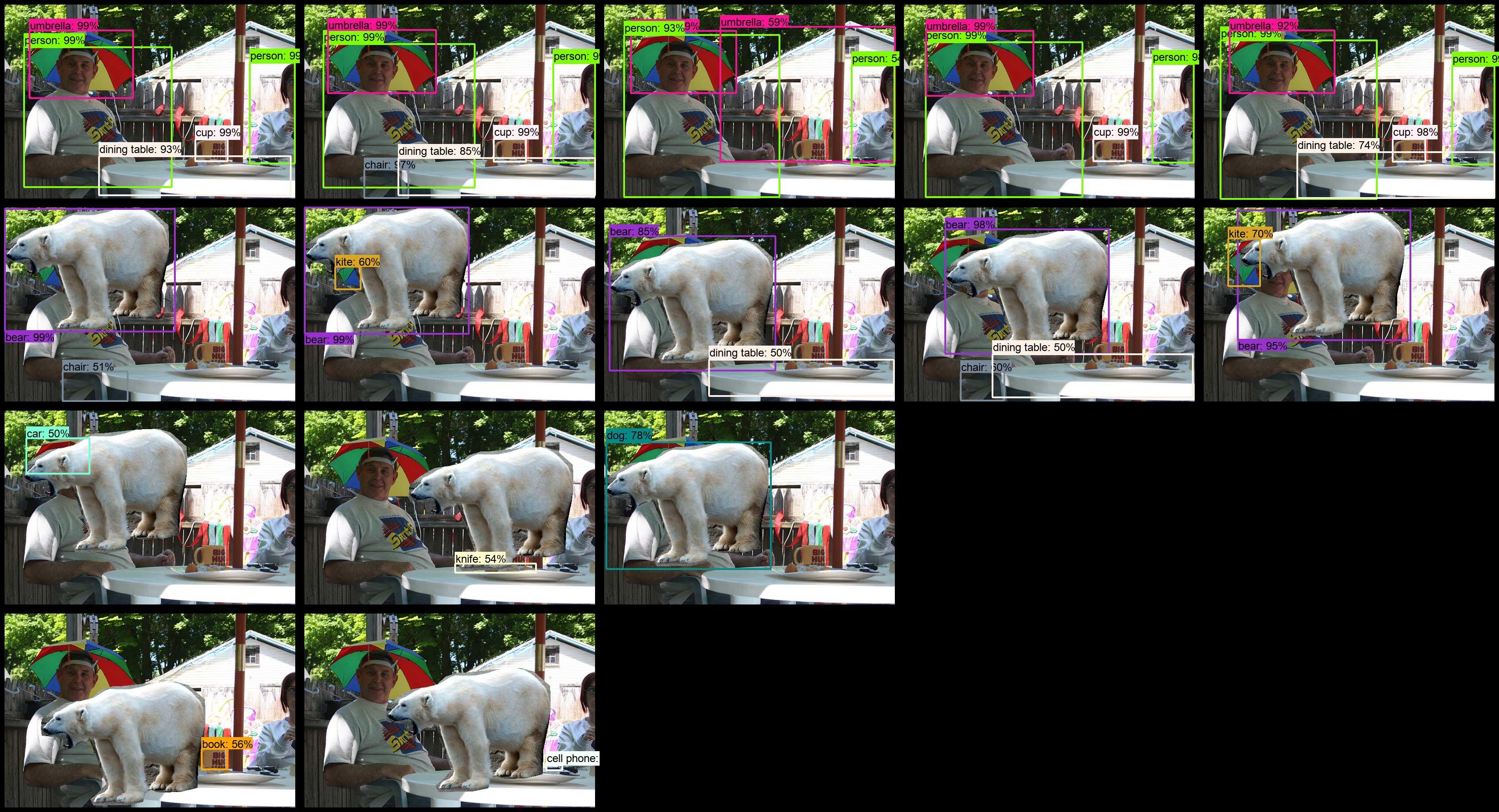
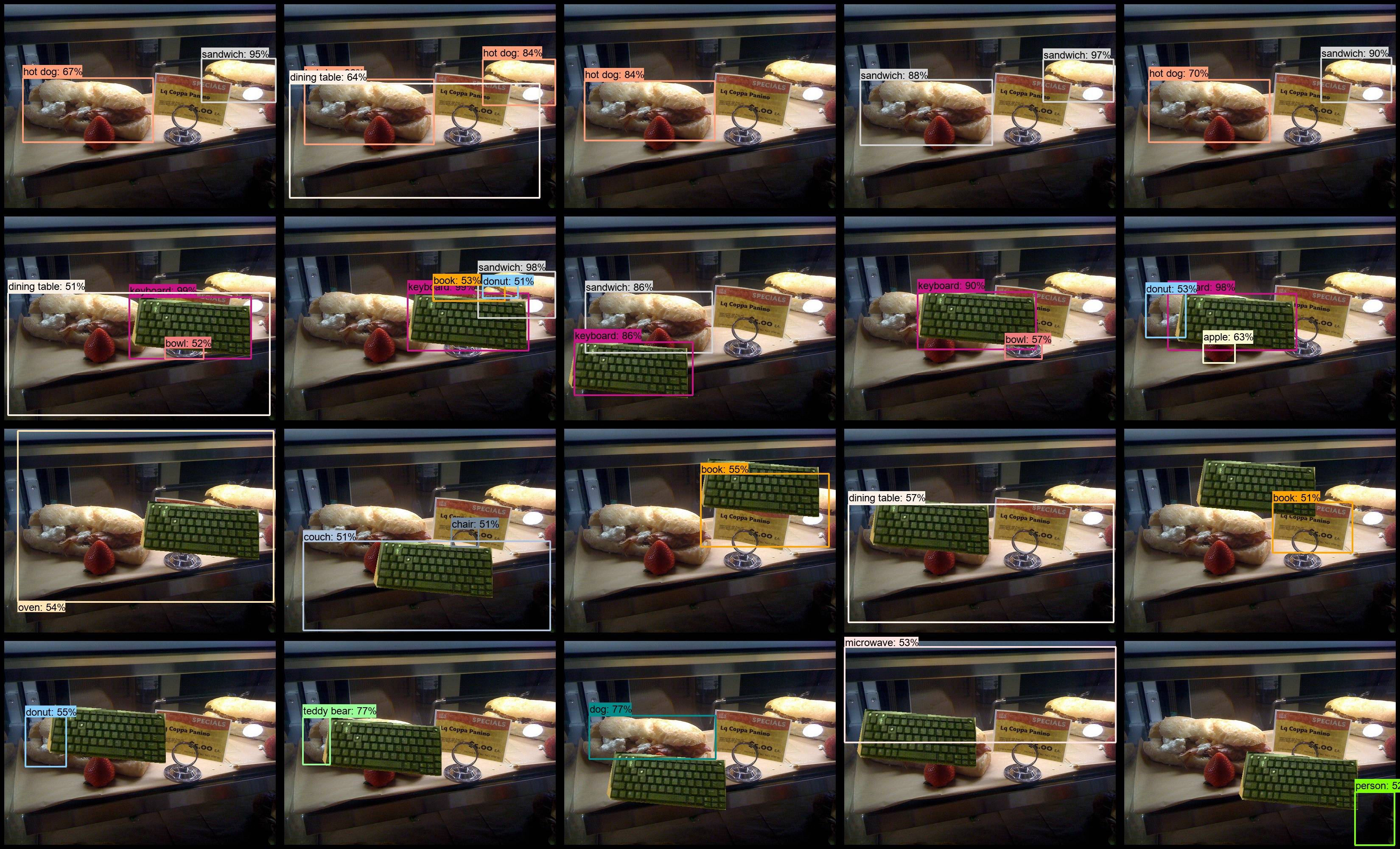
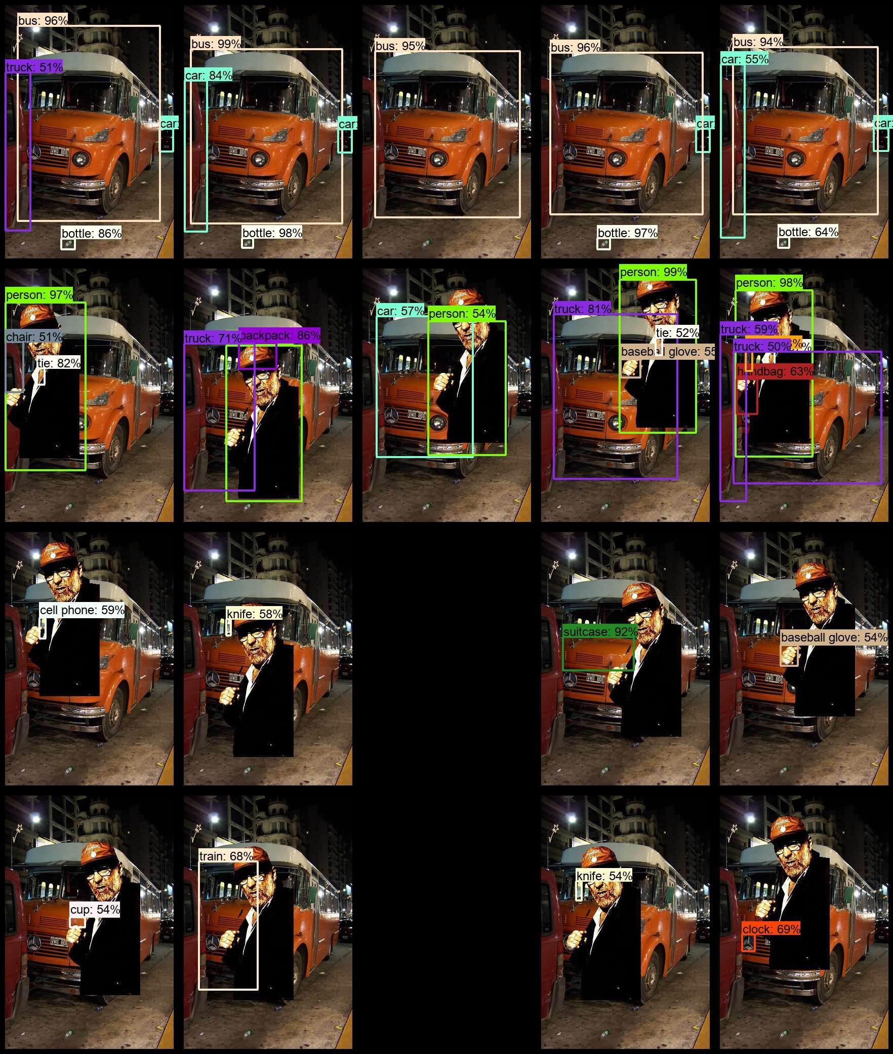
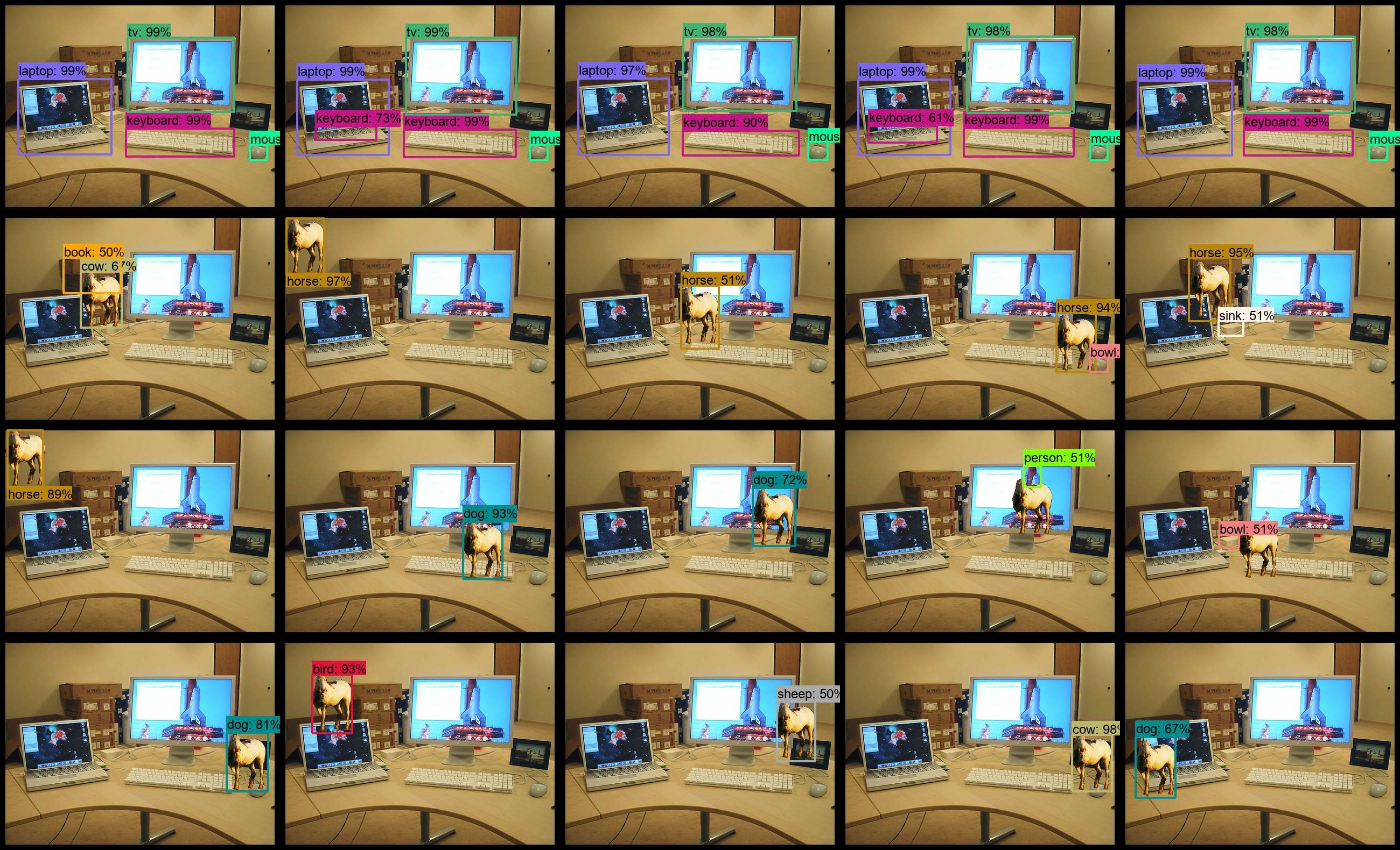
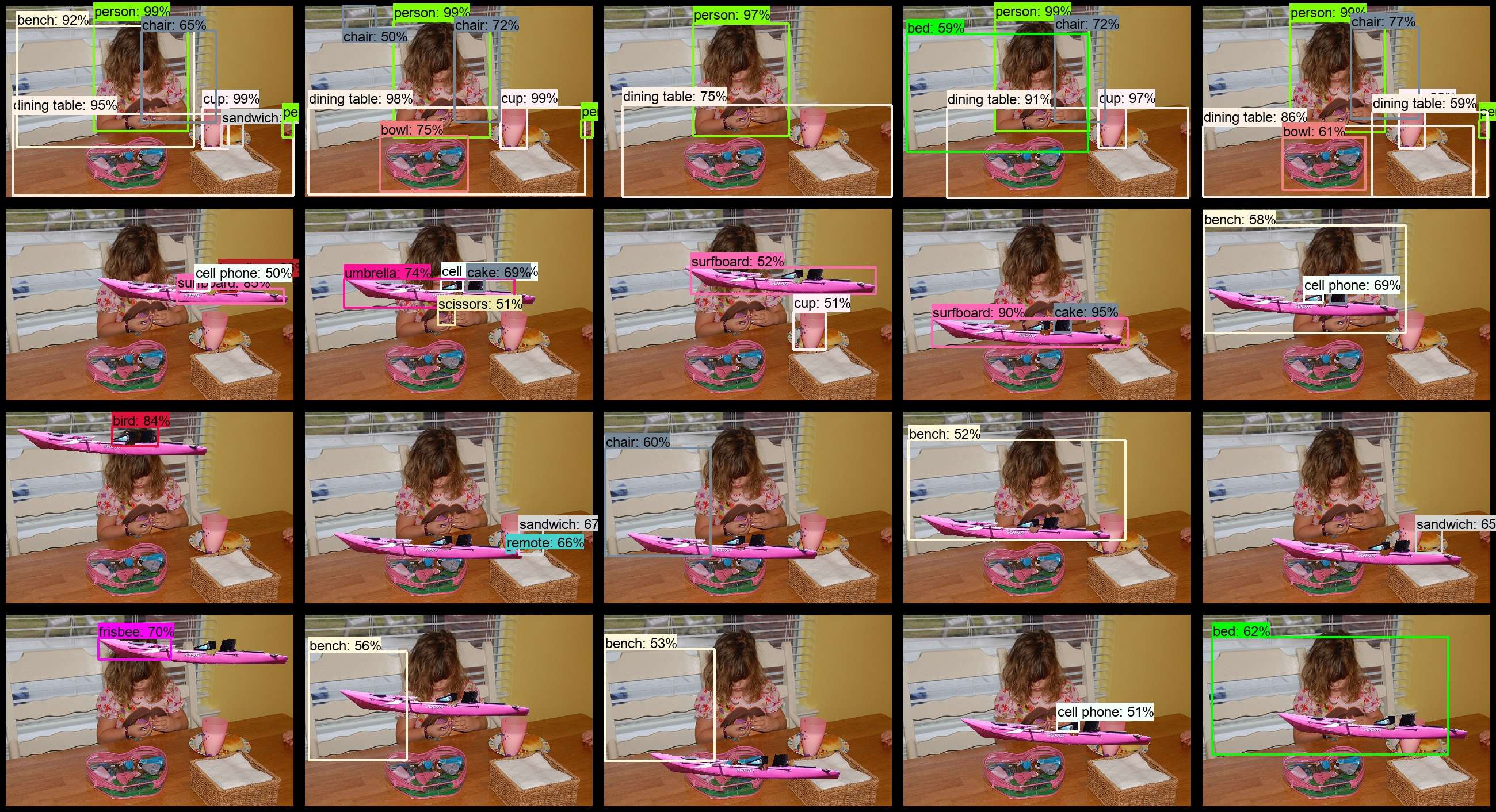
Figures 5,6,7,8,9 show detailed results of ranking a handful of the selected images according to the “Class-Matching” Criteria. We recommend viewing these figures online with zooming, as they contain many notable details. The first row of each of the figures shows the result on an unmodified image by the detectors. For each column, each successive row shows a modified image with a transplanted object, along with detection of objects whose class did not appear among the detected classes in the previous images. The order of the detectors, from left to right, is specified in the figure caption and follows that of Table II.

Let us examine Figure 6 as an interesting case. We pick to address the effects in the strongest detector, faster_rcnn_nas_coco, whose mAP is reported as 43% on the MS-COCO dataset. This is a relatively “heavy” detector, requiring 1.83s on a Titan-X GPU. For comparison, the second-best model, faster_rcnn_inception_resnet_v2_atrous_coco requires 600ms per image, roughly a third of the time, with an AP of 37%. The results of faster_rcnn_nas_coco are shown in the second column. We only show detection results with a confidence value that exceeds 0.5.

The original detection (top row, second column) shows a couple of detected hot-dogs, with the table detected as well.

The second row shows the result of adding a keyboard at a certain location. The keyboard is detected with high confidence, though now one of the hot-dogs, partially occluded, is detected as a sandwich and a doughnut. What remains visible of the small sign is now detected as a book.

The third row shows that the region below the table is now interpreted as a couch and the partially-occluded sign-holder is detected as a chair. In the last row the left hot-dog is interpreted as a teddy-bear.

We can see similar trends for the same detector in other images: in Figure 5, the bear changes the interpretation of the image so that a new kite (2nd row), knife (3rd row), cellphone (4th row) are detected for different configurations. This also happens with detectors of lower average performance. We deliberately chose to exemplify this for what is likely one of the strongest detectors currently available, showing results on additional ones for reference.

Co-occurring Objects

So far, we have shown results where the pair of images and object to be transplanted are selected randomly. Arguably, it is too much to expect a network which has never seen a certain combination of two categories within the same image to be able to successfully cope with such an image at test time. We do not believe that requiring each pair of object categories to co-occur in the training set is a reasonable one, both practically and theoretically. Certainly, it is not too much for a human. Out of context, humans are able to recognize objects, though it requires more time [2].

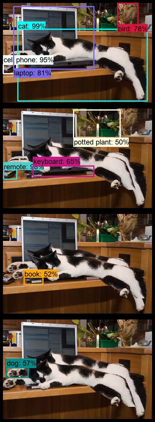
Nevertheless, we now turn to generating images of another extreme: we duplicate an object from within an image and copy it to another location in the same image. Figure 2 shows some results of detection for generated images for 4 randomly picked images. We see that the effect also happens for such images. Partial occlusions and context seem to play a role here. For example, in column (b), bottom row, the foot of the cow becomes a “remote” when near a TV. The bottom if the plant (column d, last rows 2-3) are interpreted as either a hand-bag or a cup, when part of the plant is occluded, but a person’s hand is nearby. The results in Figure 2 were all generated using the faster_rcnn_nas_coco model.

(a)

(b)

(c)

(d)

Figure 2: Effects of transplanting an object from an image into another location in the same image. Top row: original detection. Each subsequent rows: newly detected objected w.r.t to previous row, induced by the translated object copy.

Feature Interference

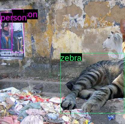
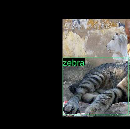
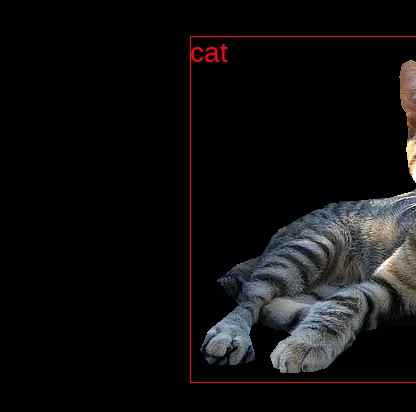
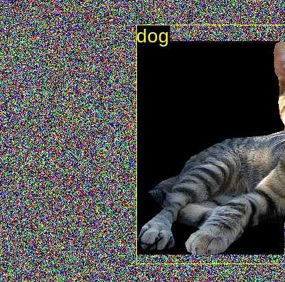
We now show how feature interference could be harmful to the detection process, as a plausible explanation to the observed detection error. As an example, consider the detection result in Figure 3 (a). A partially visible cat is detected and classified as a zebra. We demonstrate that features attained from pixels that do not belong to the actual object (cat) have an effect on the assigned class. This is true both for pixels inside the ROI (region-of-interest) of the object and for those outside of it: in Figure 3 (b) we set to zero all of the pixels outside of the bounding box. The detection result is not changed. When we also zero out the pixels inside the bounding box, leave those that belong to the cat, the resulting label becomes “cat”. This shows the effect of the pixels inside the ROI. However, when we randomize the background intensity outside the ROI, the label becomes “dog”. This shows that features from outside the ROI affect the final result of the detection. This experiment was performed with a PyTorch port of the method of Yolov3 [8], which is very fast and yields results which are on par with state-of-the-art in object detection. The final classification in this case relies on features from a single grid-cell of a convolutional layer.

(a)

(b)

(c)

(d)

Figure 3: Feature Interference. A partially visible cat is detected as a zebra (a). Discarding all pixels outside the detection’s bounding box does not fix the object’s classification, showing that features inside the region-of-interest (ROI) can cause confusion (b). Discarding also all non-cat pixels inside the ROI leads to a fixed classification (c). Adding random noise in the range outside the bounding box once again makes the detection incorrect , showing the effect of features outside the ROI (d)

Further Statistics

To gain some more insight about the spread of the reported phenomena, we take a few images and calculate statistics to summarize what happens as the transplanted object is translated over a dense set of locations, with a 5 pixels stride for each. We do this for 29 different images.

First, we count how many times the interpretation of the scene has changed from what is expected. This is done by matching the set of bounding boxes produced by the detector in the original and modified images. Recall that the set of detections of a modified image $I_{t}^{x,y}$ is denoted by $\mathcal{D}_{x,y}$ and those of the original image $I$ by $\mathcal{D_{\emptyset}}$.

We seek a maximal match between the bounding boxes of $\mathcal{D}_{x,y}$ and those of $\mathcal{D_{\emptyset}}$. A bipartite graph $\mathcal{G}$ is defined over the bounding boxes of both detection sets as the nodes. Each node corresponding to a box from $\mathcal{D}_{x,y}$ has an edge to a node from $\mathcal{D_{\emptyset}}$ only if their classes are identical. The weight $w$ is the overlap score of the corresponding boxes. A maximally weighted match $M_{x,y}$ is found. The score of the match is calculated by

$$S(M_{x,y})=\frac{\sum_{w\in M_{x,y}}w}{max(\left|\mathcal{D}_{x,y}\right|-1,\left|D_{\emptyset}\right|)}$$ (1)

Where $\left|\cdot\right|$ is the cardinality of a set. This enforces good matches both in set size and location of bounding boxes. The highest attainable score is one. The score $S$ gives us the average overlap score between each box and its matched one if there is a perfect pairing between boxes and a lower score if some boxes are missing in either set.

This allows us to count the number of objects whose detection was not affected by the transplanted object $T$. When counting $\left|\mathcal{D}_{x,y}\right|$ we in fact reduce 1 so the score will not be reduced by the detection of $T.$

For each image with a translation $I_{t}^{x,y}$, we count the image as “affected” if the $T$ at the corresponding translation gave rise to a match score below a certain threshold $\tau$. The average number of affected translations is reported in Table I for varying values of the threshold $\tau$. A higher value of $\tau$ is a more strict matching criteria. In this context, an threshold of 0.5 is quite a loose one, as we are trying to match two detections of the exact same object in the original and modified image. For very strict thresholds, i.e, $\tau=0.99$ we see that there is a very low number of bounding boxes matched the original ones exactly (less than 25%). The second row of Table I (Affected-class-Agnostic) also shows the number of affected locations if we allow two bounding boxes to match even if their classes do not. By construction this creates fewer mismatches, however not by a large margin.

	$\tau=.3$	$\tau=.5$	$\tau=.7$	$\tau=.95$	$\tau=.99$
%Affected	10.3	20.6	31.3	53.7	75.6
%Affected-class-Agnostic	6.6	15.9	25.7	52.6	75.5
%Affected-Occ-20	3.1	6.7	8.2	22.6	51.3
%Affected-No-Occ	2.4	4.5	4.95	9	22.4

TABLE I: Average effect of transplanting objects. We show the average percentage of locations where the transplanted object has caused the detection of any of the original objects to be modified, with varying strictness of matching original and modified detections (Affected). The threshold $\tau$ is the minimal overlap to count two bounding boxes of the same class as a match. A higher $\tau$ is a more strict matching criterion, leading to less matches (more affected locations). For a majority of the translations, there is no exact match between the detections on the modified and original images. Affected-class-Agnostic: results for class-agnostic matching between the bounding boxes. Affected-Occluded-20: results where we count only cases where at most 20% of the area of each original object was covered by $T$. Affected-No-Occ: results where $T$ occludes no object whatsoever.

Occlusions

The previous analysis did not consider that the object $T$ may occlude partially or fully, many of the objects in the image. Therefore, we calculate again the matching between the sets of bounding boxes while recording to which extent each of the original objects was covered by $T$. For each original bounding box $b\in D_{\emptyset}$, we calculate the coverage of $b$ by $T$ as

$$C_{b,T}=\frac{|b\cap T|}{|b|}$$ (2)

Where $|\cdot$| corresponds to the area of the bounding box (in this context $T$ is interpreted as $T$’s bounding box). We calculate the maximal coverage

$$C_{T}=\max_{b\in D_{\emptyset}}C_{b,T}$$ (3)

We calculate again the number of affected objects, this time discarding each image for which the maximal coverage $C_{T}$ exceeds 0.2. In other words, we discard all images where the object $T$ covered any object’s area by more than 20%. The results are displayed in the third row of Table I (Affected-Occ-20). The last row (Affected-No-Occ) shows the results of discarding all of the images where $T$ did not cover any of the original detections. Even in these two cases, where the objects are hardly touched by $T$ - or not at all - the object transplant still has a non-negligible effects.

Global Effects Beyond Detection

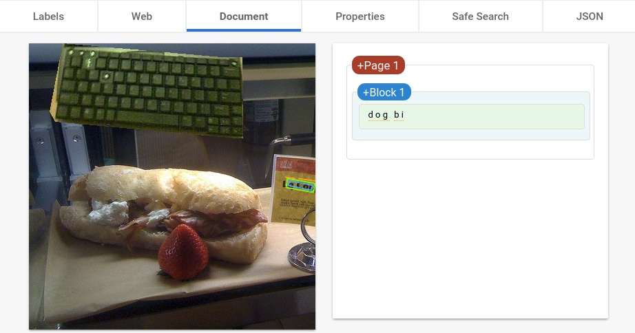
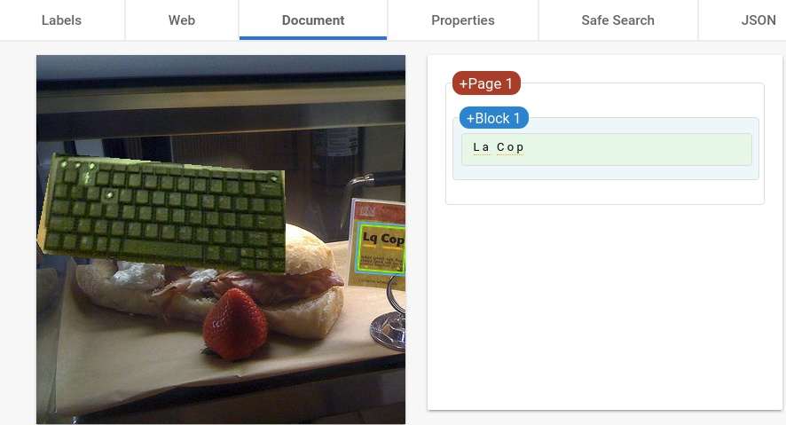
In a preliminary experiment, we uploaded a couple of the images where no object was detected at all to Google’s Vision API website. These image were picked arbitrarily. We report the result here as we find it noteworthy for further exploration. It seems that the OCR portion of their method also exhibits a surprising amount of non-local sensitivity to transplanted objects. Figure 4 shows this: the keyboard is placed in two different locations in the image. Though each of the locations is such that the keyboard is far from the sign, the interpretation of the sign is different in each case.

(a)

(b)

Figure 4: Non-local effects of object transplant on Google’s OCR. A keyboard placed in two different locations in an image causes a different interpretation of the text in the sign on the right. The output for the top image is “dog bi” and for the bottom it is “La Cop”

Discussion

We now raise several possible reasons for the observed behaviour of current object-detectors. Though there are several reported phenomenon here, we believe that there they are not independent and that some (but not all) share common underlying reasons.

Partial Occlusions

It is quite widely accepted that partial occlusions were and still are a challenge to object detectors. A good sign of generalization is being able to cope with partial occlusions. Indeed, in many of the examples that we tested, the modern object detectors were quite robust to such occlusions. In [18], this is acknowledged and a data-driven solution is proposed, implemented via an adversarial network to generate examples including occlusions and deformations. Recently, Zhang et al. [19] proposed a method to vote using local evidence in order to localize semantic parts even in heavily occluded images.

Out of Distribution Examples

It is possible that the modifies images have very low likelihood to occur under the distribution of images under the training set. Since we “paste” objects using their foreground mask onto the target image, abrupt edges are created at the patches of the object’s border. These edges may be out-of-distribution when considering the local appearance of naturally occurring edges.

The images generated here could be viewed as a variant of adversarial examples [12], in which small image perturbations (imperceptible to humans) cause a large shift in the network’s output. The images we generate are of a somewhat opposite flavor: while we do not limit the magnitude of the difference between the original and modified image, the detectors are sometimes “blind” to the inserted object, as demonstrated in Figure 1 (b,d,e,g,i). In addition, our examples are not “targeted” in the sense that no optimization process is required to generate them; they seem prevalent enough so that a simple scan of transplanting translated versions of one object in the other can give rise to multiple wrong interpretations.

(Lack of) Signal Preservation

Spatial pooling, prevalent in deep neural networks, is useful for reasons of efficiency and invariance to certain spatial deformations. However, as recently observed by Azulay and Weiss [1], these pooling layers actually prevent the network from being truly shift-invariant. Such behaviour is in fact anticipated by simple signal-processing considerations and has in fact been discussed much earlier [11]. The authors of [1] also observe that small image shifts, as well as other geometric transforms as scaling, can cause the network’s output to change dramatically.

Contextual Reasoning

It is not common for current object detectors to explicitly take into account context on a semantic level, meaning that interplay between object categories and their relative spatial layout (or possibly additional) relations) are encoded in the reasoning process of the network. Though many methods claim to incorporate contextual reasoning, this is done more in a feature-wise level, meaning that global image information is encoded somehow in each decision. This is in contrast to older works, in which explicit contextual reasoning was quite popular (see [3] for mention of many such works). Still, it is apparent that some implicit form of contextual reasoning does seem to take place. One such example is a person detected near the keyboard (Figure 6, last column, last row). Some of the created images contain pairs of objects that may never appear together in the same image in the training set, or otherwise give rise to scenes with unlikely configurations. For example, non co-occurring categories, such as elephants and books, or unlikely spatial / functional relations such as a large person (in terms of image area) above a small bus. Such scenes could cause misinterpretation due to contextual reasoning, whether it is learned explicitly or not.

Non-Maximal Suppression

Many changes to the detection results seem to be non-local. Whereas partial occlusions can be regarded as local effects of the transplanted object that directly change the object’s appearance, we also see sometimes changes in detection of objects that are far away from the transplanted object. We suggest that this may be partially due to the process of non-maxima suppression (NMS) common in object detectors: assume that a previously detected object $A$ is no longer detected due to a partial occlusion by the transplanted object $T$. An object $B$, which overlaps with $A$ and was previously suppressed during the NMS, would possibly not be suppressed now. Similar chain-reactions could cause the NMS process to eventually affect a far away object that is not adjacent to $T$.

Feature Interference

Modern object detectors use features obtained from a convolutional layer in order to generate the final object class and bounding box prediction. These regions are either fixed in size [7, 8] or rectangular. The ROI-Pooling operation [4] performs max-pooling features from sub-windows of a convolutional feature map over a region of interest (ROI). This operation is affected by the following facts:

1. The region of interest is a rectangular one. This means that sections of the region that do not belong to the object are also pooled, including background appearance as well as appearance of the object.

2. Each part of the feature map can have a large effective receptive field. In practice, this means that features are pooled from outside the bounding box of the detected object.

On one hand, including features from an object’s surroundings could provide useful contextual cues to improve object detection, especially for objects that do not provide enough evidence due to size, partial occlusion, etc. On the other hand, invariably mixing additional features into the final classification score could hinder the result.

We believe that feature interference, demonstrated in Figure 3, is perhaps the root cause for most of the observed phenomena, and that effects that seem due to partial occlusion or contextual reasoning are specific cases of this problem. Experiments discussing this difficulty have been introduced in Rosenblatt [10]. The associated problem in biological vision has later been coined the “binding problem” [17] and noted in cognitive studies in humans [13] as well. The works of Tsotsos et al. refer to this issue as cross-talk [15, 14] and predicts neural mechanisms that are in place to overcome this issue, in the form of the Selective Tuning framework. In brief, the idea is that once a first pass is finished through the visual hierarchy, the dominant signal propagates downwards through the hierarchy, performing spatial and feature attenuation so that the next pass of the signal will contain information on the object of interest that is less entangled with surrounding features. The model is discussed in more extensive details in [16] , describing the different stages of information flow through the visual hierarchy. We suggest that such mechanisms are expected to alleviate many of the observed phenomena, and leave this for future development.

Acknowledgment

This material is based upon work supported by the Air Force Office of Scientific Research under award number FA9550-18-1-0054, and by the Canada Research Chairs program through grants to JKT for which the authors are grateful.

Figure 5: Detection with Transplanted Objects. Top row : original images. Left-to-right: detection of models: faster_rcnn_inception_resnet_v2_atrous_coco, faster_rcnn_nas_coco, ssd_mobilenet_v1_coco, mask_rcnn_inception_resnet_v2_atrous_coco, mask_rcnn_resnet101_atrous_coco. Each row shows only newly added detection w.r.t the previous row in the same column to avoid clutter. Transplanting the bear causes a variety of new objects to be detected, e.g.: chair, car, book (first column); kite, knife, cellphone (second column).

Figure 6: Detection with Transplanted Objects. Top row : original images. Left-to-right: detection of models: faster_rcnn_inception_resnet_v2_atrous_coco, faster_rcnn_nas_coco, ssd_mobilenet_v1_coco, mask_rcnn_inception_resnet_v2_atrous_coco, mask_rcnn_resnet101_atrous_coco. Each row shows only newly added detection w.r.t the previous row in the same column to avoid clutter.

Model Name	COCO mAP
faster_rcnn_inception_resnet_v2_atrous_coco	37
faster_rcnn_nas_coco	43
ssd_mobilenet_v1_coco	21
mask_rcnn_inception_resnet_v2_atrous_coco	36
mask_rcnn_resnet101_atrous_coco	33

TABLE II: Models used in the reported experiments, along with their mean average precision.

Figure 7: Detection with Transplanted Objects. Top row : original images. Left-to-right: detection of models: faster_rcnn_inception_resnet_v2_atrous_coco, faster_rcnn_nas_coco, ssd_mobilenet_v1_coco, mask_rcnn_inception_resnet_v2_atrous_coco, mask_rcnn_resnet101_atrous_coco. Each row shows only newly added detection w.r.t the previous row in the same column to avoid clutter.

Figure 8: Detection with Transplanted Objects. Top row : original images. Left-to-right: detection of models: faster_rcnn_inception_resnet_v2_atrous_coco, faster_rcnn_nas_coco, ssd_mobilenet_v1_coco, mask_rcnn_inception_resnet_v2_atrous_coco, mask_rcnn_resnet101_atrous_coco. Each row shows only newly added detection w.r.t the previous row in the same column to avoid clutter.

Figure 9: Detection with Transplanted Objects. Top row : original images. Left-to-right: detection of models: faster_rcnn_inception_resnet_v2_atrous_coco, faster_rcnn_nas_coco, ssd_mobilenet_v1_coco, mask_rcnn_inception_resnet_v2_atrous_coco, mask_rcnn_resnet101_atrous_coco. Each row shows only newly added detection w.r.t the previous row in the same column to avoid clutter.

References

- [1] A. Azulay and Y. Weiss. Why do deep convolutional networks generalize so poorly to small image transformations? arXiv preprint arXiv:1805.12177, 2018.
- [2] I. Biederman. Perceiving real-world scenes. Science, 177(4043):77–80, 1972.
- [3] M. J. Choi, A. Torralba, and A. S. Willsky. Context models and out-of-context objects. Pattern Recognition Letters, 33(7):853–862, 2012.
- [4] R. Girshick. Fast r-cnn. In Proceedings of the IEEE international conference on computer vision, pages 1440–1448, 2015.
- [5] J. Huang, V. Rathod, C. Sun, M. Zhu, A. Korattikara, A. Fathi, I. Fischer, Z. Wojna, Y. Song, S. Guadarrama, et al. Speed/accuracy trade-offs for modern convolutional object detectors. In IEEE CVPR, volume 4, 2017.
- [6] T.-Y. Lin, M. Maire, S. Belongie, J. Hays, P. Perona, D. Ramanan, P. Dollár, and C. L. Zitnick. Microsoft coco: Common objects in context. In European conference on computer vision, pages 740–755. Springer, 2014.
- [7] W. Liu, D. Anguelov, D. Erhan, C. Szegedy, S. Reed, C.-Y. Fu, and A. C. Berg. Ssd: Single shot multibox detector. In European conference on computer vision, pages 21–37. Springer, 2016.
- [8] J. Redmon and A. Farhadi. Yolov3: An incremental improvement. arXiv preprint arXiv:1804.02767, 2018.
- [9] S. Ren, K. He, R. Girshick, and J. Sun. Faster r-cnn: Towards real-time object detection with region proposal networks. In Advances in neural information processing systems, pages 91–99, 2015.
- [10] F. Rosenblatt. Principles of neurodynamics. perceptrons and the theory of brain mechanisms. Technical report, CORNELL AERONAUTICAL LAB INC BUFFALO NY, 1961.
- [11] E. P. Simoncelli, W. T. Freeman, E. H. Adelson, and D. J. Heeger. Shiftable multiscale transforms. IEEE transactions on Information Theory, 38(2):587–607, 1992.
- [12] C. Szegedy, W. Zaremba, I. Sutskever, J. Bruna, D. Erhan, I. Goodfellow, and R. Fergus. Intriguing properties of neural networks. arXiv preprint arXiv:1312.6199, 2013.
- [13] A. Treisman and H. Schmidt. Illusory conjunctions in the perception of objects. Cognitive psychology, 14(1):107–141, 1982.
- [14] J. Tsotsos. Complexity Level Analysis Revisited: What Can 30 Years of Hindsight Tell Us About How the Brain Might Represent Visual Information? In Frontiers in Psychology - Cognition, 2015.
- [15] J. K. Tsotsos, S. M. Culhane, W. Y. K. Wai, Y. Lai, N. Davis, and F. Nuflo. Modeling visual attention via selective tuning. Artificial intelligence, 78(1-2):507–545, 1995.
- [16] J. K. Tsotsos, A. J. Rodríguez-Sánchez, A. L. Rothenstein, and E. Simine. The different stages of visual recognition need different attentional binding strategies. Brain research, 1225:119–132, 2008.
- [17] C. Von der Malsburg. The what and why of binding: the modeler’s perspective. Neuron, 24(1):95–104, 1999.
- [18] X. Wang, A. Shrivastava, and A. Gupta. A-fast-rcnn: Hard positive generation via adversary for object detection. In IEEE Conference on Computer Vision and Pattern Recognition, 2017.
- [19] Z. Zhang, C. Xie, J. Wang, L. Xie, and A. L. Yuille. DeepVoting: A Robust and Explainable Deep Network for Semantic Part Detection under Partial Occlusion. In Proceedings of the IEEE Conference on Computer Vision and Pattern Recognition, pages 1372–1380, 2018.
- [20] B. Zoph, V. Vasudevan, J. Shlens, and Q. V. Le. Learning transferable architectures for scalable image recognition.