Probabilistic Ensemble of Collaborative Filters††thanks: This work was done when Min was a research assistant with Lin.
Abstract
Collaborative filtering is an important technique for recommendation. Whereas it has been repeatedly shown to be effective in previous work, its performance remains unsatisfactory in many real-world applications, especially those where the items or users are highly diverse. In this paper, we explore an ensemble-based framework to enhance the capability of a recommender in handling diverse data. Specifically, we formulate a probabilistic model which integrates the items, the users, as well as the associations between them into a generative process. On top of this formulation, we further derive a progressive algorithm to construct an ensemble of collaborative filters. In each iteration, a new filter is derived from re-weighted entries and incorporated into the ensemble. It is noteworthy that while the algorithmic procedure of our algorithm is apparently similar to boosting, it is derived from an essentially different formulation and thus differs in several key technical aspects. We tested the proposed method on three large datasets, and observed substantial improvement over the state of the art, including L2Boost, an effective method based on boosting.
Introduction
Over the past decades, recommender systems have become an inherent part of e-commerce and many online sharing services. It was shown in previous study (?) that targeted recommendation is an effective way to influence customers or users and promote business. The key to a successful recommender system is the relevance of the recommendations. However, identifying products that are relevant to a user’s interest has never been a trivial task.
From a technical perspective, recommendations are usually produced by either content-based fashion or collaborative filtering. The former relies on comparing the features of an item and those rated by a given user; while the latter infers the preferences of a user based on those from other users with similar histories. In real-world applications, collaborative filtering has shown great effectiveness (?) and its success has been exemplified on the Netflix Prize (?).
On the other hand, despite the extensive studies devoted to improving collaborative filters, the performances of current collaborative filtering techniques remain unsatisfactory in a number of practical applications. A key challenge lies in the diversity of the real-world data. Take the books sold on Amazon for example. Different customers may purchase a book for different reasons – some may find the story interesting while others are perhaps just attracted by the authors. In collaborative filtering, each item is encoded by a fixed vector, and so is each user. Such a formulation may not be able to provide the needed capacity to capture the diverse ways in which users may evaluate an item.
A natural idea to improve the capability of handling diverse data is to construct an ensemble, which can combine multiple predictors specialized in different kinds of data. Ensemble methods, as an important family of techniques in machine learning, have been extensively studied (?; ?), and shown to be very effective for a number of tasks (?; ?). However, the use of ensemble methods for recommendation remains relatively limited. Most of the approaches (?; ?) just work in a vanilla weighted-sum fashion.
With these challenges in mind, we develop a new method for constructing a collaborative filter ensemble. Unlike existing methods for this task (?), our method is based on a probabilistic generative model, in which the latent embeddings for both items and users are generated from a prior distribution, and the predictions are then derived from a distribution conditioned on the given embeddings. With this setting, an ensemble can thus be formalized as a mixture model, of which each component is a probabilistic predictor. On top of this formulation, we further derive a progressive construction algorithm. This algorithm begins with a basic collarborative filter. Then in each iteration, it tries to obtain a new one that is complementary to the current ensemble by learning from a re-weighted set. The new predictor will then be incorporated into the ensemble. It is worth noting that using this progressive method, one need not prescribe the size of the ensemble, i.e. the number of component filters. The algorithm can proceed until the performance saturates or the ensemble reaches the maximum allowed size.
We evaluated the proposed method on three large datasets, MovieLens (?), CiteULike (?), Netflix (?), comparing it with other recommendation methods, especially those for constructing collaborative filter ensembles. Experimental results showed that our method consistently outperforms others on all three datasets. We also conducted a series of ablation studies to investigate how different modeling choices influence the overall performance.
Related Work
Among the various approaches for constructing predictor ensemble, Boosting methods such as AdaBoost and L2Boost (?; ?; ?), show great capability and have been widely used in practice. AdaBoost works in a stage-wise manner. At each iteration, misclassified samples are assigned with higher weights and a new predictor is trained on the re-weighted set. Note that AdaBoost was developed for binary classification and thus is not directly applicable for collaborative filtering. But its underlying idea has inspired a series of other boosting formulations. L2Boost, on the other hand, aims to fit the raw data distribution, specifically with L2 Loss. Thus it is very suitable for regression tasks. More recently in (?), L-EnsNMF was proposed for topic modeling. It is an ensemble approach combining Nonnegative Matrix Factorization and gradient boosting. Besides, general ensemble theories have also been an active topic in recent years (?; ?; ?).
Along another track, Matrix co-clustering methods, which were originally introduced to explore the blocking structure of a matrix, have also been applied to construct ensembles of collaborative filters (?; ?), driven by the intuition that for different subgroups of users and items, the matching relations between them can be different and may need to be modeled differently. Recently, Lee et al proposed LLORMA (?; ?), with the assumption that a rating matrix is low-rank locally (i.e. within sub-matrices). Based on a related idea, Beutel et al proposed ACCAMS together with its Bayesian counterpart bACCAMS (?). ACCAMS is an iterative KMeans-style algorithm, while bACCAMS is a generative Bayesian non-parametric model. The most recent progress is CCCF (?), which adopts a probabilistic method to model overlapped coclusters, and parallelizable MCMC for scalable inference. We note that the methods mentioned above were mostly devised for approximating real-valued matrix rather than collaborative filtering implicit feedback. Our experiments show that direct application of such methods to recommendation tasks often results in suboptimal performance.
In addition, Deep Learning methods are also attracting more and more attention (?; ?). However, we will not be discussing them since such methods generally require outer features while ours is focused on the ratings alone.
Formulation
Collaborative filtering is an important technique for recommendation (?; ?), and has been widely used in practical systems.
A widely adopted formulation for collaborative filtering is based on embeddings. Specifically, given a finite set of users and items, respectively denoted by and , it associates each user with an embedded vector and each item an embedded vector . Then, we can compute the matching score between them based on the dot product between the corresponding embedded vectors, as .
The embedding vectors are usually obtained by fitting the matching scores to the observed ratings on a training set. A popular method for this is Weighted Matrix Factorization (WMF) (?). It solves the embedding vectors by minimizing the following objective function:
| (1) |
Here, is the confidence coefficient for the observed rating , and are regularization coefficients. Sometimes in practice, a portion of ratings will be omitted in the training stage, for which the coefficient will be set to zeros.
Let denote the user embedding matrix of size , the item embedding matrix of size , the (observed) rating matrix with , and the confidence coefficient matrix with . Then the objective function in Eq. (1) can be rewritten into a matrix form as
| (2) |
Here, denotes element-wise product, and the Frobenius norm. The optimal solutions to and can be solved using alternate coordinate descent.
Probabilistic Formulation
As mentioned, the expressive power of a classical collaborative filter is limited when applied to highly diverse data. A natural idea to mitigate this problem is to construct an ensemble of filters, each specialized to a certain kind of data. Towards this goal, we explore a probabilistic formulation of collaborative filters(?). As we will see, this formulation can be readily extended to an ensemble-based framework and will result in an efficient and elegant learning algorithm.
Specifically, from a probabilistic perspective, a collaborative filter can be viewed as a conditional distribution as , where the distribution of the rating depends on the and , namely the latent embeddings of a user and an item. Based on this notion, we can formulate a probabilistic model that explains the entire generative process, including the generation of the embeddings and that of the ratings. The model is described as follows:
-
1.
For each user , draw an embedding .
-
2.
For each item , draw an embedding .
-
3.
For each pair , draw the rating from the conditional distribution .
Here, is the prior variance of the embeddings. Given a training set with partially observed ratings, the problem is to estimate the embeddings and . This can be done via Maximum-A-Posterior (MAP) estimation, which is to maximize the objective function given below with respect to and :
| (3) |
Here, is the confidence coefficient for the pair , and is the probability density function for the embedding prior . The conditional distribution is formulated as a normal distribution centered at , as:
| (4) |
It is not difficult to see that under this setting, the learning problem as formulated in Eq. (3) reduces to a Weighted Matrix Factorization (WMF) problem as in Eq. (1), with the regularization coefficient given by .
Extension to Ensembles
From a mathematical standpoint, the probabilistic formulation introduced above is equivalent to the classical WMF formulation. Moreover, this new formulation can be readily extended to an ensemble model, via probabilistic mixture modeling.
Specifically, an ensemble of collaborative filters can be considered as a probabilistic mixture model, comprising generative components. In particular, each component has its own set of embeddings for users and items. According to this setting, the conditional distribution of the rating for the pair is given by
| (5) |
Here, and are respectively the embeddings for the -th user and the -th item, with the -th component filter, and . In addition, this mixture model also comes with a prior distribution over the components in the ensemble, and is the prior probability for the -th component.
Generally, like other probabilistic mixture models, the model above can be estimated from a set of training data using the Expectation-Maximization (EM) algorithm (?). In our context, the EM algorithm alternates between E-steps and M-steps. Particularly, the E-step computes the posterior probability of the pair being generated from the -th component, conditioned on the embeddings produced by the last iteration, as
| (6) |
Note that the probability values are normalized such that for every pair . These probability values can also be considered as a set of “soft weights” that associate each pair with different components.
The M-step, instead, updates the embeddings for each component based on a re-weighted WMF. Particularly, for the -th component, it can be updated by solving the following problem.
| (7) |
Compared to the standard WMF given by Eq. (1), the only change here is that the coefficient is replaced by . Therefore, the problem can be solved similarly. The M-step also updates the prior probabilities as .
Progressive Construction Algorithm
While the EM algorithm presented above is a standard way to estimate mixture models, we found empirically in our study that it does not work very well for the recommendation task. A key issue here is that the component filters initialized randomly (i.e. on a random partition of the ratings) are not sufficiently complementary. While the E-M updates can optimize them to a certain extent, they are pretty much trapped in a suboptimal configuration.
For an ensemble model to work, the key is complementarity, namely, to maintain a diverse set of components that are complementary to each other. In this work, we develop a new algorithm for constructing an ensemble of collaborative filters. Instead of having all components randomly initialized at the very beginning and then performing iterative updates, it constructs the ensemble in a progressive manner, that is, to add one component at a time. Each new component will be learned to complement the current ensemble, with focus placed on those entries that are not well predicted.
Overall Procedure
Specifically, this algorithm begins with a standard WMF predictor, with all observed entries weighted equally. The first component may produce reasonable predictions for a considerable portion of ratings. However, for a diverse dataset, there can be certain parts that are not well predicted. New components will be introduced in following iterations to reinforce them.
Next, the key question is how to derive a new component that can complement the current ensemble. In particular, suppose the current ensemble gives a conditional distribution , as in Eq. (5). Now, we want to add one filter . If we assign a weight to the new component and thus a weight to the existing ensemble, then the combined distribution would be:
| (8) |
This is similar to a finite mixture model, except that this mixture contains exactly two components, an existing ensemble and a new filter, and that the first component is fixed. Hence, we can estimate with a restricted version of the EM algorithm:
-
1.
Compute the association weights to both components for each observed pair . Here, we denote the posterior weight to the new component by , and thus the weight to the existing ensemble is .
-
2.
Estimate the new component based on the re-weighted pairs, where the coefficient for the pair is .
Computing
.
It is important to note that when computing the posterior weights , the embeddings of the new component are still unavailable and thus needs to be marginalized out. The marginalized conditional distribution for the new component is
| (9) |
By the symmetry of the formulation, the value of is a constant that does not depend on and . Hence, we can simply denote it by . Therefore, with the new embeddings marginalized out, for the pair , the posterior probability of being from the new component is given by
| (10) |
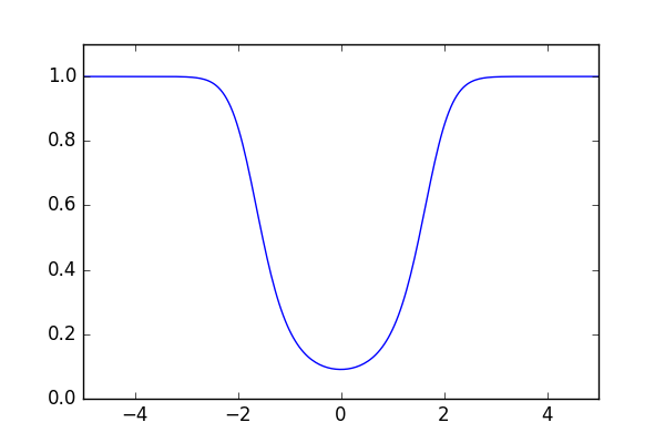
Let , then . Consequently, the new filter can be constructed based on a re-weighted distribution, where the ratings at is associated with a coefficient , as mentioned above. Note that in our formulation, , where is the prediction error of the current ensemble for the pair . Then, the weight is actually a function of the current prediction error , as shown in Fig.1. We can see that when is relatively small, increases quadratically as increases, which means that the algorithm tends to assign a pair to the new component when it is not well predicted. Also, the value of will saturate to as continues to increase.
It is noteworthy that the function here is controlled by two design parameters: (1) controls the (prior) tendency of assiging samples to the new component; and (2) controls the bandwidth of the weighting curve. With a smaller value of , the weight would saturate more quickly as the error increases.
Discussions
Compared to the standard EM algorithm, the progressive method presented above has several advantages:
-
1.
It encourages complementarity when each new component is being constructed. This is reflected by the weighting function . Particularly, a large prediction error by the current ensemble would result in a greater weight towards the new component. The experimental results in the next section will show that this scheme is more effective than EM.
-
2.
It does not require , the number of components, to be specified in advance. One can continue to add new filters to the ensemble until the prediction performance is satisfactory or the ensemble reaches the maximum allowed size.
-
3.
The computation complexity for the weights is constant, i.e. it does not depend on the number of components. It makes it scalable to very large ensembles.
The major computational cost of the proposed method lies at the estimation of new CF components. This cost grows linearly as the number of components increases. Note that during inference, all the components can run in parallel, so the method can scale well in a parallel or distributed environment when deployed for practical service.
Experiments
We conducted experiments to test our method on three real-world datasets that cover different application domains and have different rating densities. In this section, we first introduce the datasets, evaluation metrics, and the baseline methods, then present the comparative results and the findings from ablation studies.
Datasets
| user# | item# | entry# | density | |
|---|---|---|---|---|
| MovieLens | 27.7K | 6.4K | 1.8M | 1.00% |
| CiteULike | 5.6K | 17.0K | 0.21M | 0.22% |
| Netflix | 19.5K | 13.1K | 6.3M | 2.48% |
| MovieLens | CiteULike | Netflix | |||||||
|---|---|---|---|---|---|---|---|---|---|
| Recall@50 | Recall@100 | Recall@200 | Recall@50 | Recall@100 | Recall@200 | Recall@50 | Recall@100 | Recall@200 | |
| bACCAMS | 0.213 | 0.348 | 0.525 | 0.073 | 0.125 | 0.220 | 0.080 | 0.151 | 0.270 |
| WMF | 0.377 | 0.540 | 0.698 | 0.388 | 0.494 | 0.594 | 0.142 | 0.271 | 0.452 |
| L2Boost | 0.418 | 0.566 | 0.705 | 0.416 | 0.513 | 0.607 | 0.178 | 0.312 | 0.480 |
| PECF | 0.460 | 0.606 | 0.747 | 0.446 | 0.545 | 0.645 | 0.258 | 0.390 | 0.550 |
The three datasets in our experiments are described below.
-
1.
MovieLens is derived from the MovieLens 20M Dataset (?). It is a large public benchmark with about million ratings. Removing the users and movies which occur very rarely in the dataset, the resultant set contains users and movies. We treat all five-star ratings as positive while others as zeros. Then the overall rating density is about .
-
2.
CiteULike, provided in (?), is a dataset about researchers and the papers they are interested in. Researchers can add the articles that they found relevant into their respective personal libraries. The author-paper associations in this context are typical implicit feedback. This dataset contains researchers and papers. The overall density is around .
-
3.
Netflix is the official dataset used in the Netflix Prize competition (?). The original dataset consists of about million movie ratings, from users and for movies. Given the limited computation budget we have, we construct a subset with only the frequent users and movies. This subset contains users and items. Similar to above, we treat all five-star ratings as positive. The rating density for this set is around .
The basic statistics of these datasets are summarized in Table 1. To construct the training, validation, and testing sets, we randomly split the ratings (both the positive and zeros) into three disjoint parts by the ratio 3:1:1. These parts are respectively for training, validation and testing. We employ NVIDIA Titan X GPUs to accelerate matrix computation.
Performance Metrics
In previous work, various metrics have been used to evaluate the performance of recommenders. However, as pointed out in (?), recall is more suitable than precision in the context of recommendation with implicit feedback, as some positive pairs would be missing from the groundtruths. For example, a user might be truly interested in an item but did not provide a rating as he/she was unaware of it. Hence, we follow the metric recall in our experiments. Specifically, for each user, we sort all the items in descending order of the predicted scores, and select the top items to recommend. Recall@M is defined as:
We report the Recall@M metric averaged over all users. In our experiments, ranges from to . It is worth noting that the Recall@M metric also imitates how recommenders are used in the real-world services.
To provide a complementary perspective, we also use Weighted Mean Square Error (WMSE) as an additional metric, which is defined as
where is exactly the confidence coefficient used in WMF. indicates that WMSE is evaluated only over the entries in the testing set. This metric directly measures how well the predicted scores match the ground-truths.
Methods to Compare
Below are all the methods we compared in our experiments.
-
1.
WMF. Weighted Matrix Factorization (WMF) (?) is a popular collaborative filtering technique and often used as a baseline in literatures. It derives the latent embeddings for both users and items through regularized matrix factorization of the rating matrix .
-
2.
ACCAMS. Additive Co-Clustering to Approximate Matrices Succinctly (ACCAMS) was proposed in (?) for matrix approximation. In this paper, a Bayesian version called bACCAMS was also developed. This method attempts to find local co-clusters of rows and columns to approximate a given matrix. Here, we apply to the rating matrix to obtain local collaborative filters. In our experiment, we will test the performance of bACCAMS.
-
3.
L2Boost+WMF. L2Boost (?) is a variant of boosting that aims to minimize the L2 loss. It works in a stage-wise manner. In each stage, it fits a new component to the residue of the current ensemble. In order to reduce the risk of overfitting and also leave space for subsequent training, a shrinkage parameter is usually added for a newly trained predictor.
-
4.
PECF, Probabilistic Ensemble of Collaborative Filters (PECF) is our method presented in this paper. PECF constructs an ensemble of filters progressively. In each iteration, a new filter is trained on re-weighted entries in order to complement the current ensemble. In the experiments, we want to compare it with the methods listed above.
Detailed Settings: In our experiments, we follow the conventional practice to set the confidence coefficient in WMF, with for positive entries and for zero entries. For bACCAMS, we randomly sample of the missing entries as the negative label. The latent embedding dimension is determined respectively on different datasets via cross validation. Particularly, we set to for MovieLens, for CiteULike, and for Netflix. These settings are used for WMF, L2Boost and PECF for fair comparison. In addition for iterative methods, including L2Boost and our method, we limit the number of training cycles to be at most . As for the design parameters and in our method, we set them to and via cross validation.
Quantitative Comparison
| Recall@50 | Recall@100 | Recall@200 | ||
|---|---|---|---|---|
| PECF | 0.453 | 0.601 | 0.745 | |
| 0.460 | 0.606 | 0.747 | ||
| 0.457 | 0.602 | 0.743 | ||
| L2Boost | 0.418 | 0.561 | 0.701 | |
| 0.418 | 0.566 | 0.705 | ||
| 0.418 | 0.552 | 0.690 | ||
Table 2 compares the performances of different methods on all three datasets in terms of the Recall@M metric. The experimental results suggest:
-
1.
Ensemble methods, including L2Boost and our method PECF, can notably improve the recall as compared to the WMF baseline. Particularly, PECF can deliver remarkable performance gains over a single WMF filter. On MovieLens dataset, Recall@50 is promoted from to (around of relative gain). On CiteULike, Recall@50 is promoted from to (around of relative gain). The improvement on Netflix is even more significant, where Recall@50 is promoted from to , with the relative gain at .
-
2.
Among the three datasets, Netflix has the highest density, but the lowest Recall. It is partly due to the complex and ambiguous patterns in this dataset. However, our method shows great cability of handling such complicated cases.
-
3.
The performance of bACCAMS, which was originally developed for real-valued matrix approximation, is clearly inferior to other methods under the implicit feedback setting. Especially on CiteULike, the extremely low density of the dataset leads to the poor Recall of bACCAMS.
In what follows, we will examine our method in detail, in order to study how different design parameters influence the overall performance.
| Recall@50 | Recall@100 | Recall@200 | |
|---|---|---|---|
| 0.460 | 0.606 | 0.747 | |
| 0.450 | 0.598 | 0.742 | |
| 0.435 | 0.590 | 0.738 | |
| 0.431 | 0.586 | 0.735 |
Ablation Studies
We conducted ablation studies to investigate the influence of several design parameters: the number of components, the latent dimension, the re-weighting parameters and , as well as the weight of new component .
Number of components
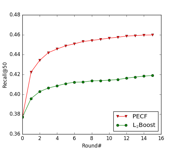
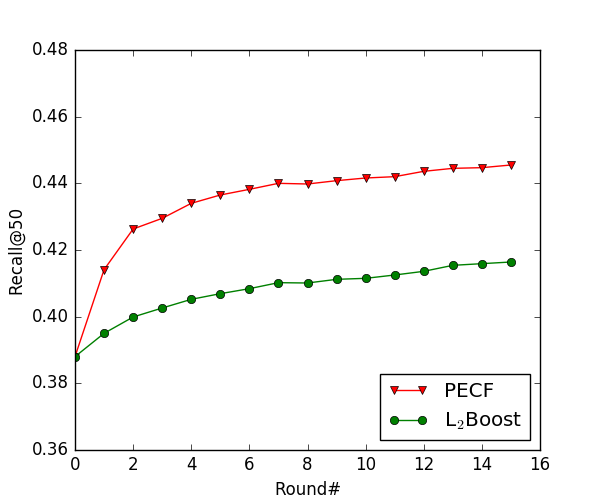
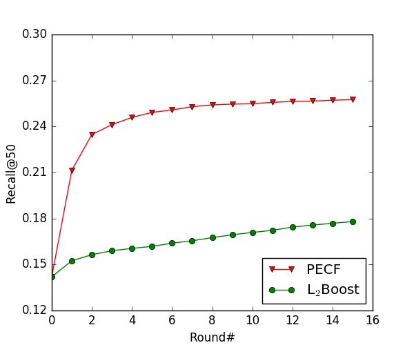
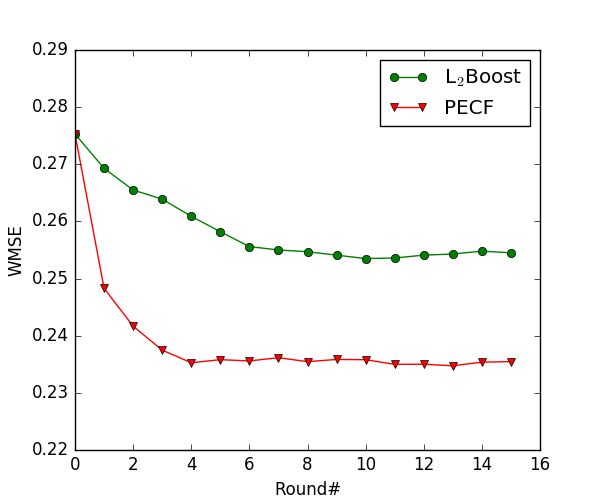
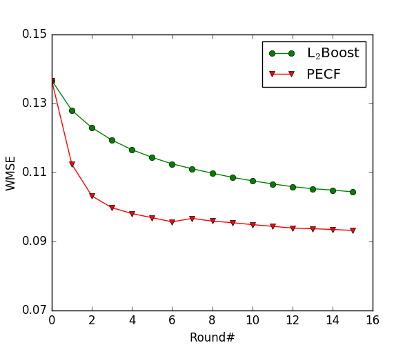
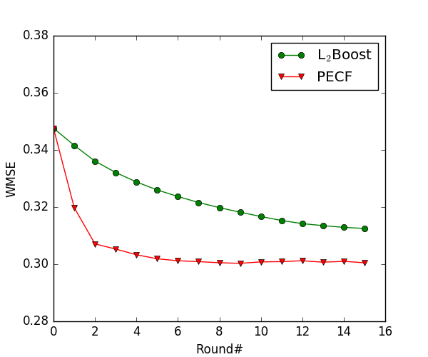
Both L2Boost and PECF construct an ensemble progressively. They add a new component at each round. Here, we study how the number of new components, i.e. the number of training rounds, affects the overall performance, in both Recall@50 and WMSE. The result is shown in Fig. 2. Note that in these figures, when , the model is exactly a single WMF predictor.
First, we can see that WMSE metric is consistent with Recall@50. As mentioned, implicit feedback problems are difficult to tackle. A common solution is to treat it as a regression task and employ weighted L2 Loss during training. This consistency between WMSE and Recall in our experiments implies that the choice of weighted L2 loss as the training objective is appropriate.
We can also see that the progressive construction leads to stable improvements, both for L2Boost and PECF. Especially at the first few rounds, the improvements resulted from PECF is substantial. Compared to L2Boost, PECF not only converges faster, but also outperforms consistently and by a notable margin.
Latent embedding dimension
Now we will investigate how the latent dimension influences the overall performance, for both PECF and L2Boost.
On MovieLens dataset, as mentioned, the best result is attained when . Table 3 show the results when is set to , , and respectively. We can see that the results are at a comparable level and not of significant difference. This implies that naively increasing the latent dimension does not lead to better results. As we have argued, PECF works in a progressive manner, and newly trained predictor works as an complementary to the current ensemble. Whereas the parameter size may be similar to a WMF predictor with higher latent dimension, the key difference lies in the way of how individual components are trained.
Re-weighting parameter and
In addition, we also study the influence of re-weighting parameter and the bandwidth paramter on MovieLens in Table 4. Particularly, controls the tendency of assigning user/item pairs to new components, while determines the bandwidth of the weighting function .
We can see that the best result is attained at and . The re-weighting curve is shown exactly in Fig. 1, where gradually saturates after 2. In fact, we empirically found that most of the predictions lie before saturation, and the new weight is very similar to a vanilla quadratic function of the error . Those points residing out of the bandwidth can be viewed as outliers and the saturation suppressed their impact, thus resulting in more reliable training.
New component weight
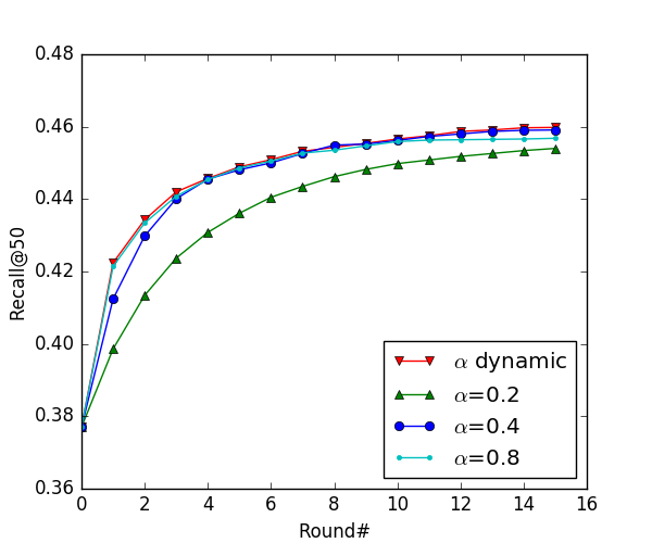
In our model, the mixture parameter is determined dynamically, in a way that is similar to line search in steepest gradient descent. In this part, we will see the comparison with fixed , and the results on MovieLens are shown in Fig. 3.
For fix settings, smaller and larger values of respectively have their own limitations. In particular, when , the result is still slightly increasing and has not completely converged, and this is surely not an ideal situation as it requires longer training time; when , the Recalls at the last few rounds are similar to dynamic setting, but performs worse at the first few rounds; when , the initial converging rate is competitive, but the final converge value is not as satisfied. Overall, setting dynamically at each round is the best strategy.
Comparison to EM Algorithm
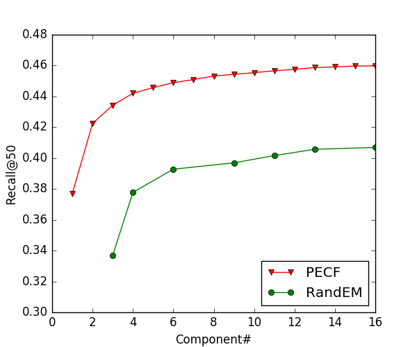
As mentioned, the ensemble is a mixture model that can be trained using the EM algorithm, first initialized and later updated in parallel. The proposed PECF method works in a progressive manner, adding one complementary component at a time. Fig. 4 show the results of both ways on MovieLens, which compare the performance of both algorithms under different number of components. In this figure, the EM algorithm with random initialization is referred to as RandEM, and L2EM for initialization from L2Boost.
We observe: (1) Both algorithms can improve the performance as the number of components increases; (2) RandEM performs substantially worse than our construction method. This is partly ascribed to the reason that for RandEM, components are randomly initialized, and not explicitly encouraged to be complementary. This experiment, again, suggests the importance of complementarity in ensemble learning.
Conclusion
This paper presented a new method to construct an ensemble of collaborative filters for recommondation. It is based on a probabilistic mixture formulation. But unlike previous work that usually adopts EM estimation, we develop a progressive algorithm that explicitly encourages complementarity among component filters. Experiments on three large datasets, namely MovieLens, CiteULike, and Netflix, show that the proposed method not only leads to significant performance gain over a single collaborative filter, but also outperforms other ensemble-based methods, including L2Boost and bACCAMS, by considerable margins. It is noteworthy that our method is a generic approach to ensemble construction. While we adopt WMF as the basic component in this paper, our method can also work with other predictors as the basic components.
Acknowledgement
This work is partially supported by the Big Data Collaboration Research grant from SenseTime Group (CUHK Agreement No. TS1610626), the General Research Fund (GRF) of Hong Kong (No. 14236516).
References
- [Bennett, Lanning, and others 2007] Bennett, J.; Lanning, S.; et al. 2007. The netflix prize. In Proceedings of KDD cup and workshop, volume 2007, 35. New York, NY, USA.
- [Beutel, Ahmed, and Smola 2015] Beutel, A.; Ahmed, A.; and Smola, A. J. 2015. Accams: Additive co-clustering to approximate matrices succinctly. In Proceedings of the 24th International Conference on World Wide Web, 119–129. ACM.
- [Bühlmann and Hothorn 2007] Bühlmann, P., and Hothorn, T. 2007. Boosting algorithms: Regularization, prediction and model fitting. Statistical Science 477–505.
- [Bühlmann and Yu 2003] Bühlmann, P., and Yu, B. 2003. Boosting with the l 2 loss: regression and classification. Journal of the American Statistical Association 98(462):324–339.
- [Dempster, Laird, and Rubin 1977] Dempster, A. P.; Laird, N. M.; and Rubin, D. B. 1977. Maximum likelihood from incomplete data via the em algorithm. Journal of the royal statistical society. Series B (methodological) 1–38.
- [Dietterich 2000] Dietterich, T. G. 2000. Ensemble methods in machine learning. In International workshop on multiple classifier systems, 1–15. Springer.
- [Friedman et al. 2000] Friedman, J.; Hastie, T.; Tibshirani, R.; et al. 2000. Additive logistic regression: a statistical view of boosting (with discussion and a rejoinder by the authors). The annals of statistics 28(2):337–407.
- [Friedman 2001] Friedman, J. H. 2001. Greedy function approximation: a gradient boosting machine. Annals of statistics 1189–1232.
- [Harper and Konstan 2016] Harper, F. M., and Konstan, J. A. 2016. The movielens datasets: History and context. ACM Transactions on Interactive Intelligent Systems (TiiS) 5(4):19.
- [Hu, Koren, and Volinsky 2008] Hu, Y.; Koren, Y.; and Volinsky, C. 2008. Collaborative filtering for implicit feedback datasets. In Proceedings of the 2008 Eighth IEEE International Conference on Data Mining, 263–272. IEEE Computer Society.
- [Lacoste et al. 2014] Lacoste, A.; Marchand, M.; Laviolette, F.; and Larochelle, H. 2014. Agnostic bayesian learning of ensembles. In Proceedings of The 31st International Conference on Machine Learning, 611–619.
- [Lee et al. 2013] Lee, J.; Kim, S.; Lebanon, G.; and Singer, Y. 2013. Local low-rank matrix approximation. In Proceedings of The 30th International Conference on Machine Learning, 82–90.
- [Lee et al. 2016a] Lee, J.; Kim, S.; Lebanon, G.; Singer, Y.; and Bengio, S. 2016a. Llorma: Local low-rank matrix approximation. Journal of Machine Learning Research 17(15):1–24.
- [Lee et al. 2016b] Lee, S.; Prakash, S. P. S.; Cogswell, M.; Ranjan, V.; Crandall, D.; and Batra, D. 2016b. Stochastic multiple choice learning for training diverse deep ensembles. In Advances in Neural Information Processing Systems, 2119–2127.
- [Mnih and Salakhutdinov 2008] Mnih, A., and Salakhutdinov, R. R. 2008. Probabilistic matrix factorization. In Advances in Neural Information Processing Systems, 1257–1264.
- [Rendle et al. 2009] Rendle, S.; Freudenthaler, C.; Gantner, Z.; and Schmidt-Thieme, L. 2009. Bpr: Bayesian personalized ranking from implicit feedback. In Proceedings of the twenty-fifth conference on uncertainty in artificial intelligence, 452–461. AUAI Press.
- [Shaham et al. 2016] Shaham, U.; Cheng, X.; Dror, O.; Jaffe, A.; Nadler, B.; Chang, J.; and Kluger, Y. 2016. A deep learning approach to unsupervised ensemble learning. In Proceedings of The 33rd International Conference on Machine Learning, 30–39.
- [Suh et al. 2016] Suh, S.; Choo, J.; Lee, J.; and Reddy, C. K. 2016. L-ensnmf: Boosted local topic discovery via ensemble of nonnegative matrix factorization. In Proceedings of IEEE 16th International Conference on Data Mining, ICDM 2016, December 12-15, 2016, Barcelona, Spain, 479–488.
- [Wang and Blei 2011] Wang, C., and Blei, D. M. 2011. Collaborative topic modeling for recommending scientific articles. In Proceedings of the 17th ACM SIGKDD international conference on Knowledge discovery and data mining, 448–456. ACM.
- [Wang, Wang, and Yeung 2015] Wang, H.; Wang, N.; and Yeung, D.-Y. 2015. Collaborative deep learning for recommender systems. In Proceedings of the 21th ACM SIGKDD International Conference on Knowledge Discovery and Data Mining, 1235–1244. ACM.
- [Wu et al. 2016] Wu, Y.; Liu, X.; Xie, M.; Ester, M.; and Yang, Q. 2016. Cccf: Improving collaborative filtering via scalable user-item co-clustering. In Proceedings of the Ninth ACM International Conference on Web Search and Data Mining, 73–82. ACM.
- [Xu et al. 2012] Xu, B.; Bu, J.; Chen, C.; and Cai, D. 2012. An exploration of improving collaborative recommender systems via user-item subgroups. In Proceedings of the 21st international conference on World Wide Web, 21–30. ACM.
- [Xue et al. 2005] Xue, G.-R.; Lin, C.; Yang, Q.; Xi, W.; Zeng, H.-J.; Yu, Y.; and Chen, Z. 2005. Scalable collaborative filtering using cluster-based smoothing. In Proceedings of the 28th annual international ACM SIGIR conference on Research and development in information retrieval, 114–121. ACM.
- [Zheng, Noroozi, and Yu 2017] Zheng, L.; Noroozi, V.; and Yu, P. S. 2017. Joint deep modeling of users and items using reviews for recommendation. In Proceedings of the Tenth ACM International Conference on Web Search and Data Mining, 425–434. ACM.