Application of Bounded Total Variation Denoising in
Urban Traffic Analysis

Abstract

While it is believed that denoising is not always necessary in many big data applications, we show in this paper that denoising is helpful in urban traffic analysis by applying the method of bounded total variation denoising to the urban road traffic prediction and clustering problem. We propose two easy-to-implement methods to estimate the parameter noise strength in the denoising algorithm, and apply the denoising algorithm to GPS-based traffic data from Beijing taxi system. For the traffic prediction problem, numerical experiments show that the predicting accuracy is improved by applying the proposed bounded total variation denoising algorithm. For the clustering problem, we apply a recently developed parameter-free clustering analysis method for more than one hundred urban road segments in Beijing based on their velocity profiles. Much better clustering results are obtained after denoising.

65M10, 78A48

1 Introduction

Transportation has become an important part in our everyday life, which brings many kinds of traffic problems at the same time. For example, big cities like Beijing have a trend to be more and more congested as the enormous growing of private cars. Many researchers have tried to analysis and alleviate the traffic congestion problem with different methods, especially using vehicle information from Global Positioning System (GPS) as more and more GPS data are available. GPS data has been used for exploring the cause and propagation of traffic jams [1, 2], mining the fastest driving route [3], trying clustering methods for trajectories to characterize patterns of traffic [4, 5], estimating the volume of citywide transportation [6], predicting the taxi destinations [7] and forecasting the velocity [8, 9]. All of these works are based on trajectories and have utilized temporal, spatial or spatio-temporal properties. In this paper, we are interested in velocity prediction. As we all know if the speed is much lower than the average velocity of vehicles on a road for a relatively long time, then there is a high possibility that congestion is formed. So accurate traffic velocity forecast is the base for routine planning, congestion control and analysis, etc.. However, such a traffic forecast is not an easy task in practice as a result of both the limit of methods and data volume and quality. Urban traffic is a quite complex system, leading that data collected contain noise. Noises may come from two aspects. On the one hand, due to the number of cars appearing on an urban road in a short time interval is very limited, one needs to consider the average number of cars and the average velocity on a given road as stochastic processes. On the other hand, measurement error and processing error(e.g. the GPS mapping error) may be introduced in the data collection and post-processing procedures. Correspondingly, there are two ways to deal with noisy data. One is to treat noise as real, and develop new methods to improve accuracy(see, e.g., [8, 9, 7, 4, 5]). The other is to first reduce noise in the collected data [10], and then use the denoised data to forecast on the base of existing methods [11, 12].

In this paper, we prefer to the latter way mentioned above. The reasons are as follows. First, data can be used in urban traffic analysis without expensive cost are often sparse comparing to the complexity of the problem. So we need to make the limited data effective rather than using the noisy data directly. Second, although some existing methods have some tolerance with noise, like deep neural network [13, 14]. The real performance of the network depends on many factors and we believe these methods will perform better with proper-denoised data under the same condition. In fact, some neural network methods are not robust to noise [15], which causes overfitting. Many methods are proposed to prevent overfitting, like early stopping, regularization, soft weight sharing[16], denoising autoencoders[17, 18] and dropout[19, 20]. Third, by using dedicated and robust denoising algorithms, shallow neural networks and other simple models using less data can give fairly good urban traffic prediction, which is favorable in real-time and online applications comparing to deep neural networks due to their efficiency.

There exist many useful methods developed for image and video denoising, such as [21, 22, 23, 24, 25, 26, 27, 28, 29, 30, 31, 32, 33, 34, 35, 36, 37, 38]. Some of these methods have been applied to traffic analysis, e.g. the wavelet method [11, 39] and the compressive sensing method [10, 40, 12]. These methods work fairly well in some denoising applications, but they are based on particular assumptions on noise and specific basis functions. We want to use a method works well with less assumptions on noise and basis functions and the parameters of which are easy to obtain. Thus we apply bounded total variation (BV) denoising method [21] to urban traffic velocity data. It has edge preserving property [41], which is consistent with the sudden jump of traffic speed. Our goal is to find the reconstructed velocity in the function space of bounded total variation and estimate the noise strength during the process of denoising with less assumptions on the type of noise. To this end, we propose two efficient methods to estimate the noise strength, which almost do not request any assumptions on noise.

The rest of the paper is organized as follows. In section 2, we first review the method of BV denoising, then show how to apply the BV denoising method to traffic data by proposing two different ways to estimate the noise strength. In section 3, we show the effectiveness of denoising by applying the proposed methods to Beijing urban road velocity data derived from taxi GPS system. We end the paper with some concluding remarks in section 4.

2 The BV denoising algorithm for traffic velocity data

In this section, we first give a brief introduction to the method of BV denoising, and then show how to apply it to traffic velocity data.

2.1 BV denoising model

Let $u_{0}(x)$, $x\in\Omega\subseteq\textbf{R}^{d}$ be the original observed velocity vector and $u(x)$ be the denoised velocity vector. Then $u_{0}(x)=u(x)+\xi(x)$, where $\xi(x)$ is the noise whose mean is 0. We first consider the BV denoising method for continuous case and then discuss the corresponding discrete case. For the continuous case, the BV denoising method is to find the solution $u$ by solving the following optimization problem [21]

$$\min_{u(x)}\operatorname{TV}(u)=\min_{u(x)}\int_{\Omega}|\triangledown u(x)|dx$$ (1)

such that

$$\int_{\Omega}\!u(x)dx=\int_{\Omega}\!u_{0}(x)dx,\qquad\frac{1}{2}\!\int_{\Omega}\!\big{(}u(x)-u_{0}(x)\big{)}^{2}dx=\sigma^{2},$$ (2)

where $\sigma$ is the noise strength parameter need to be specified. When we apply the BV denoising method to reduce the noise in road velocity time series, $x$ is one dimensional, so we only consider the case that $d=1$ below. The first order condition of the optimization problem satisfies (2) and following Euler-Lagrange equation:

$$\frac{d}{dx}\Big{(}\frac{u_{x}}{|u_{x}|}\Big{)}-\lambda_{1}-\lambda_{2}(u-u_{0})=0,\qquad\frac{\partial u}{\partial n}\Bigr{|}_{\partial\Omega}=0,$$

where $u_{x}=\frac{\partial u}{\partial x}$, $\lambda_{1}$ and $\lambda_{2}$ are the corresponding Lagrange multipliers. To obtain the solution of the optimization problem (1), one can solve the following equations corresponding to the gradient flow of the Lagrange function with respect to $u$:

$$u_{t}=\frac{d}{dx}\Big{(}\frac{u_{x}}{|u_{x}|_{\epsilon}}\Big{)}-\lambda_{2}(u-u_{0}),$$ (3)

$$\frac{\partial u}{\partial n}\Bigr{|}_{\partial\Omega}=0,$$ (4)

$$u(x,0)=u_{0}(x)+\sigma\phi,$$ (5)

where $\phi$ in (5) satisfies $\mathbb{E}(\phi)=0$, $\frac{1}{2}\int_{\Omega}\phi^{2}dx=1$ such that $u(x,0)$ satisfies the constraint (2), and $|x|_{\epsilon}=|x|+\epsilon$ with $\epsilon$ is a relatively small number to avoid singularity and obtain better numerical stability. In addition, when initial condition (5) is used, we can assure $\lambda_{1}=0$ all the time. So we discard $\lambda_{1}$ and only keep $\lambda_{2}$, which is rewritten as $\lambda$ for simplicity. To calculate $\lambda$, we first multiply $u(x)-u_{0}(x)$ on both sides of (3), then integrate the result on $\Omega$. By the Neumann boundary condition and (2), we obtain:

$$\lambda=\frac{1}{2\sigma^{2}}\int_{\Omega}\frac{u_{x}}{|u_{x}|_{\epsilon}}\cdot((u_{0})_{x}-u_{x})dx.$$ (6)

$\lambda$ changes as $u_{x}$ changes with respect to $t$, and converges when $t$ goes to infinity [21, 42].

The steady state solution of (3)-(4) represents the clean data denoised from the observed data $u_{0}(x)$. Next, we present numerical schemes to solve equations (3)-(4) in discrete case.

2.2 The projected gradient descent algorithm

The data we used are average traffic velocities on urban roads derived from the taxi GPS records. If we have a velocity record every other 5 minutes each day, then we have 288 records for each road every day. However, the velocity records are often less than 288 for most roads because of the limit of taxi numbers and recording equipments. Therefore, we make nearest interpolation for missing data such that each road has 288 velocity records each day. In this way, we set $N=288$, and let $x$ direction correspond to direction of $N$ time slices. Define

$$\frac{1}{2}\sum_{i=1}^{N}(u(x_{i})-u_{0}(x_{i}))^{2}\cdot h=\sigma_{d}^{2},$$ (7)

where $h$ is the duration of time intervals, in which the traffic velocity on road segments are averaged. For the data we used, $h$ is 5 minutes. $x_{i}=[(i-1)h,ih)$, $i=1,2,\ldots,N$ are the time intervals in one day, $u_{0}(x_{i}),u(x_{i})$ are the observed and denoised velocity for time slice $i$, $\sigma_{d}$ corresponds to the noise strength in discrete case. While $\sigma$ and $\sigma_{d}$ are different, we do not distinguish them in the following for convenience.

We use projected gradient descent(PGD) method [42] to find the numerical solution of equations (3)-(4) because it is relatively straightforward and good enough for our goal in this study. It is guaranteed that the PGD method converges [43]. We note that there exist several more advanced numerical algorithms for complicated denoise problems, such as the Bregman iterative algorithms [26, 28, 33] and augmented Lagrangian method [29, 44], etc.

Denote $u_{i}^{n}=u(x_{i},t^{n})$, where $n$ is the iteration index, $\Delta t^{n}=t^{n+1}-t^{n}$ is the step size of the $n$-th iteration. The detailed projected gradient descent bounded variation denoising (PGDBV) algorithm is described as follows.

Algorithm PGDBV: The algorithm takes the observed velocity series: $\left\{u_{0}(x_{i}),\ i=1,\ldots,N\,\right\}$; the variance of the noise: $\sigma$; the maximum iteration number: $N_{iter}$; the relative tolerance of gradient decay: $\delta$ as input. The denoised velocity series: $\left\{u_{i},\ i=1,\ldots,N\right\}$, and the total variation of denoised data: $V$ are calculated by performing the following steps.

1. Initialize velocity series: $u^{0}_{i}=u_{0}(x_{i}),i=1,\ldots,N$, and calculate the initial discrete total variation:

   $$V^{n}=\operatorname{TV}(u^{n})=\sum_{i=1}^{N-1}|u^{n}_{i+1}-u^{n}_{i}|,$$ (8)

   with $n=0$. If $V^{n}=0$, then set $u_{i}=u_{i}^{0},i=1,\ldots,N$, $V=V^{0}$ and return.

2. For $n$ from $0$ to $N_{iter}-1$, do the following iterations

   1. Update the Lagrange multiplier $\lambda^{n}$ as

      $$\lambda^{n}=\frac{{h}}{2\sigma^{2}}\sum_{i=1}^{N-1}\frac{\triangle^{+}u_{i}^{n}}{|\triangle^{+}u_{i}^{n}|_{\epsilon}}(\triangle^{+}(u_{0})_{i}-\triangle^{+}u_{i}^{n}),$$

      where $\Delta^{+}u^{n}_{i}:=u^{n}_{i+1}-u^{n}_{i}$.

   2. Calculate the gradient of the $i$-th segment as

      $$g_{i}^{n} =-\Bigl{(}\frac{1}{h}\bigl{(}\frac{\triangle^{+}u_{i}^{n}}{|\triangle^{+}u_{i}^{n}|_{\epsilon}}-\frac{\triangle^{+}u_{i-1}^{n}}{|\triangle^{+}u_{i-1}^{n}|_{\epsilon}}\bigr{)}-\lambda^{n}(u_{i}^{n}-u_{0}(x_{i}))\Bigr{)},\quad\mbox{for}\ i=1\ldots N,$$

      where $\triangle^{+}u_{0}^{n}=0$, and $\triangle^{+}u_{{N}}^{n}=0$.

   3. Obtain step size $\triangle t^{n}$ with line search;

   4. Update the variable $u^{n+1}=u^{n}-\triangle t^{n}g^{n}$;

   5. Calculate the total variation $V^{n+1}$ using (8) with $n$ replaced by $n+1$;

   6. If $\|g^{n}\|_{\infty}/V^{0}\leq\delta$, then set $u_{i}=u_{i}^{n+1},i=1,\ldots,N,\;V=V^{n+1}$ and return.

3. Set $u_{i}=u_{i}^{N_{iter}},i=1,\ldots,N,\;V=V^{N_{iter}}$ and return.

2.3 Estimate of the noise strength

In Algorithm PGDBV, input $\sigma$ is a characterization of the noise strength. But we do not know its value a priori. Now we propose two different ways to estimate $\sigma$.

Method 1: Multi-resolution noise estimate.

In each day, every road has $N=288$ velocity records corresponding to $N$ time slices. We want to estimate the noise strength in three different resolutions: $N_{1}=N$, $N_{2}=\frac{N}{2}$, $N_{3}=\frac{N}{4}$. Denote $[N]=\{1,2,\cdots,N\}$. Let

$$v_{i}^{0}=u_{0}(x_{i}),\;i\in[N_{1}];\qquad v_{i}^{j}=\frac{v^{j-1}_{2i}+v^{j-1}_{2i-1}}{2},\;i\in[N_{j+1}],\;j=1,2.$$ (9)

Then the variation in three resolutions are:

$${V_{j+1}=\sum_{i=1}^{N_{j+1}-1}|v^{j}_{i+1}-v^{j}_{i}|^{2}\cdot\frac{1}{2^{j}h},\quad j=0,1,2.}$$

The estimate of $\sigma$ together with an error bound is given in the following Theorem. The proof can be found in Appendix.

Theorem 2.1.

Assume $u_{0}(x_{i})=u_{i}+\xi_{i},i\in[N]$, where $\xi_{i}$ is independent with $\xi_{j}$ for $i\neq j$, $\mathbb{E}(\xi_{i})=0$, $\mathbb{E}(\xi_{i}^{2})=\frac{2\sigma^{2}}{Nh}$, $i\in[N]$, then

$$\hat{\sigma}^{2}=h^{2}\frac{(\frac{119}{16}-\frac{27}{4N})V_{1}+(\frac{9}{4N}-\frac{49}{16})V_{2}+(\frac{9}{2N}-\frac{35}{8})V_{3}}{\frac{3577}{128}+\frac{189}{8N^{2}}-\frac{819}{16N}},$$ (10)

is a consistent estimate of $\sigma$, in the sense that

$$\mathbb{E}｛(\hat{\sigma}^{2})｝-\sigma^{2}=h^{2}\frac{(\frac{49}{16}-\frac{9}{4N})(V_{1}^{c}-V_{2}^{c})+(\frac{35}{8}-\frac{9}{2N})(V_{1}^{c}-V_{3}^{c})}{\frac{3577}{128}+\frac{189}{8N^{2}}-\frac{819}{16N}},$$ (11)

where

$$V_{j+1}^{c}=\sum_{i=1}^{N_{j+1}-1}\frac{|u^{(j)}_{i+1}-u^{(j)}_{i}|^{2}}{2^{j-1}h},\quad\mbox{for}\ j=0,1,2,$$

with $u_{i}^{(0)}=u_{i},i\in[N_{1}]$, $u_{i}^{(j)}=\frac{u_{2i-1}^{(j-1)}+u_{2i}^{(j-1)}}{2},i\in[N_{j+1}],j=1,2.$

Remark 2.2.

From the representation of $\mathbb{E}(\hat{\sigma}^{2})$ in Theorem 2.1, it can be seen $\hat{\sigma}$ depends on $h$. If $h$ is smaller, then the estimation can be closer to the real unknown $\sigma$.

We now use two examples to test the ability of the method above: 1) $u(x)=\sin(\pi x)$, $x=[-1,1]$, $h=\frac{2}{N}$; 2) $u(x)=\max(1-|x|,0)$, $x=[-1,1]$, $h=\frac{2}{N}$. We add white noise whose standard deviation is $\sigma$ such that the signal-to-noise ratio is 3. Test results are in Table 1. From Table 1, we found that the numerical results of proposed method for estimating $\sigma$ are very good. However, some assumptions on noise are required in this method. Next, we present a method use less assumptions.

Table 1: Numerical Results of Noise Estimate Using Method 1.

	$u(x)=\sin(\pi x)$				$u(x)=\max(1-|x|,0)$
$N_{l}$	288	144	72		288	144	72
$\sigma$	0.4941	0.4446	0.4385		0.4127	0.4176	0.3992
$\hat{\sigma}$	0.4896	0.4558	0.4646		0.4089	0.4290	0.3813
$Bias(N_{l})$	2e-6	1.69e-5	1.47e-4		4.47e-7	3.59e-6	2.89e-5
$\hat{\sigma}^{2}/\sigma^{2}-1$	-0.0182	0.0508	0.1230		-0.0182	0.0554	-0.0878

Method 2: a balance between $\sigma$ and $TV$.

From the BV denoising model, we see that when $\sigma=0$, $TV(u)=TV(u_{0})$. As $\sigma$ increases, $TV$ decreases, and eventually goes to $0$. In this process, a critical point exists at which the decreasing speed of $TV$ has a significant slow down . We regard this point as $\hat{\sigma}$, and give a quantitative way to identify it. Choose some values for $\sigma$ in increasing order first. And for any two successive $\sigma_{1}$ and $\sigma_{2}$, $\sigma_{1}<\sigma_{2}$, calculate the variance $\delta(TV(\sigma_{2})\cdot\sigma_{2}^{2})$ as

$$\delta(TV(\sigma_{2})\cdot\sigma_{2}^{2}))=TV(\sigma_{2})\cdot\sigma_{2}^{2}-TV(\sigma_{1})\cdot\sigma_{1}^{2}.$$ (12)

Plot the result of $\delta(TV(\sigma)\cdot\sigma^{2})$ against $\sigma^{2}$. Then find the $\sigma$ where $\delta(TV(\sigma)\cdot\sigma^{2})$ reaches the local minimum value for the first time, and regard it as the value for $\hat{\sigma}$. We use $\delta(TV(\sigma_{2})\cdot\sigma_{2}^{2})$ as an index because $TV(\sigma_{2})\cdot\sigma^{2}_{2}$ increases first and then decreases with the increase of $\sigma_{2}$. The first stage is mainly due to noise reduction, but in the second stage some of the real $TV$ is removed. So we need a good threshold. By some numerical tests, we found that the location where the increment gets its first local minimum is a good choice.

We have presented two methods to estimate noise strength ${\sigma}$. However, both of them have advantages and disadvantages. The first method is easier to apply, but the estimation result depends on some related assumptions. The second method does not need any assumption on noise, but it is heuristic. To get a better estimate, we combine the two methods together. Let $\hat{\sigma}_{1}$, $\hat{\sigma}_{2}$ denote the estimated noise strength with Method 1 and 2. Denote the maximum, minimum velocity $v_{\max}$, $v_{\min}$ for a road in a day. Then take $TV_{l}=\frac{5}{2}(v_{\max}-v_{\min})$ as a lower bound of $TV$. If the $TV$ corresponding to $\min(\hat{\sigma}_{1},\hat{\sigma}_{2})$ is less than $TV_{l}$, then let $\hat{\sigma}$ be the $\sigma$ corresponding to $TV_{l}$, otherwise $\hat{\sigma}=\min(\hat{\sigma}_{1},\hat{\sigma}_{2})$.

3 Experiments

In this section, we use taxi GPS data of Beijing to demonstrate the performance of our method. There are 288 time slices in one day, each is 5-minute long. If no GPS record appears in some slice, we get no velocity record in that time slice. In general, if one method performs well in a randomly chosen domain of Beijing, then it can be extended to other domains. Therefore, we randomly choose an area from Beijing and consider the GPS records for roads in it. First, we choose 24 roads at random from this fixed domain, with road length not less than 100 meters and daily record number not less than 150. The results for more roads are similar, the reason we choose 24 roads is to show the results in limited page space. We use the 24 roads to test the estimated noise strength with methods proposed in section 2 and combine them together to obtain the best estimate. After that, the velocity of these 24 roads before and after denoising on a fixed day are presented to give a visual effect directly. In further, we use history matching to prove that predicting accuracy is improved after denoising with the best estimated noise strength. Second, 102 roads in the chosen domain, whose length is not less than 100 meters and velocity records are not less than 120, are put together to see the denoising effect on clustering. As a result, a satisfactory clustering consequence is obtained after denoising.

3.1 Estimated best noise strength

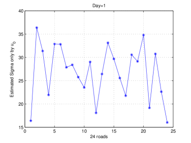
We carry out experiments on the 24 roads for 8 days, and only present some related results on the first day in this part since the results for other days are similar. Day 1 to 8 correspond to March 4-8, 18-19, 11, 2013, all of which are weekdays. Since there are time slices without velocity record, we use linear nearest interpolation and matrix completion methods [45, 46] to complete the missing values. The estimated $\sigma$ for the 24 roads on Day 1 with two different kinds of treatments for missing data by Method 1 are shown in Figure 1, which shows that the differences are small.

Figure 1: Estimated $\sigma$ by Method 1 using different methods for missing values (Left: Nearest interpolation; Right: Matrix completion).

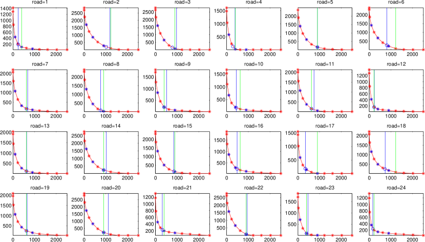
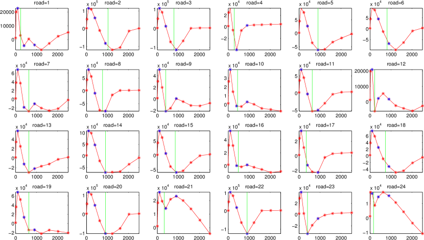
Then we estimate noise strength with Method 2. First, Figure 2 shows the relationship between $TV$ and $\sigma^{2}$, where the horizontal and vertical axis represent $\sigma^{2}$ and $TV$ respectively. The values of $\sigma$ are $0,1$ and every other 5 from $5$ to $50$, totally 12 numbers. In this figure, red star points correspond to the 12 values of $\sigma^{2}$, and blue star points denote the cases for $\sigma^{2}=[10^{2},20^{2},30^{2}]$. It can be discovered that, for each road, $TV$ is decreasing with the growth of $\sigma^{2}$. The quantitative way to identify $\hat{\sigma}_{2}$ in Method 2 is demonstrated in Figure 3, where the horizontal axis is the value of $\sigma^{2}$, and vertical axis is $\delta(TV(\sigma)\cdot\sigma^{2})$. For example, the abscissa of the first point on road 1 is $\sigma=1$, and its ordinate is $\delta(TV(1)\cdot 1^{2})$. $\hat{\sigma}_{2}^{2}$ is the location where $\delta(TV(\sigma)\cdot\sigma^{2})$ reaches minimum value for the first time. For road 1, this minimal point is reached at $\sigma=20$, which implies $\hat{\sigma}_{2}=20$. In Figure 3, the intersection of the green line with the horizontal axis is the best estimated $\sigma^{2}$. The results of combining the two methods together is also shown in Figure 2, where the values of $\hat{\sigma}_{1}$, $\hat{\sigma}_{2}$ are the intersections of the blue, green vertical line and the horizontal axis separately. And blue circle points are the best estimates for noise strength. It can be seen from Figure 2 that all the best estimates for the noise strength lie in $(\hat{\sigma}_{2}-5,\hat{\sigma}_{2}+5)$ except road 17 and 18. Therefore, the criterion we chosen in method 2 is appropriate.

Figure 2: Relationship figure for $TV$ and $\sigma^{2}$ on Day 1.

Figure 3: Estimated $\sigma$ for the 24 roads on Day 1 with Method 2.

3.2 Velocity before and after denoising

We show the velocity before and after denoising on Day 1 with best chosen $\sigma$ for the 24 roads in Figure 4, where blue and red points represent the velocity before and after denoising respectively. Nearest interpolation is used to handle missing values. From Figure 4, we can say we have reduced much noise in the velocity indeed. Specifically, the velocity vector is much smoother after denoising than that of before denoising. And the velocity after denoising keeps the peak values, such as the peak in the morning and evening. In addition, it can be observed that when the original velocity has a sudden jump, the denoised velocity also has a jump almost at the same time, which is clearly observed on road 21 and 24. Namely to say, our denoising method can keep the jump when the original velocity has a sudden ascending or descending, which is very important in urban traffic prediction and analysis. This is consistent with the edge preserving property of bounded total variation method. On the other hand, the denoising effect of some roads, like road 3, 8, 22, are not that obvious as others although the performance is better than the original velocity. This may be caused by their location. They are close to intersections and are all assistant roads, which have big spatial noise, while we only consider temporal noise.

Figure 4: Velocity before and after denoising for the 24 roads on Day 1. The horizontal axis is 288 time slices, and the vertical axis is the velocity value.

3.3 Validation by history matching

We have seen the denoising effect directly above. Now we validate that this denoising method helps in velocity prediction. We first make a nearest interpolation to assure there are 288 records every day for all the chosen roads. Data of the first 7 days are regarded as history data, and the prediction part is from Day 8. We realize it based on history matching. Specifically, we break the history data daily into vector of length 4 in terms of time series. Take Day 1’s data for example, 282 vectors are obtained. The first one of them is the velocity records from time slice 1 to 4, and the last one is that of time slice 282 to 285. And the velocity vector after 15 minutes is from time slice 7 to 288 respectively. Therefore, 1974 input vectors of length 4 and corresponding labels of length 1 are gained for the history part. And for Day 8’s data, the goal vector for time slice $K$ is formed by velocity of time slice $K-3$ to $K$. We make use of a popular clustering algorithm [47] (more details in the last part of this section) to cluster for the 1974 input vectors and the goal vector. The distance between two vectors is measured by $l^{2}$ norm. After that, we regard the Gaussian-weighted average of those labels, whose input vectors are in the same cluster with the goal vector, as the velocity prediction.

What we described above is exactly the prediction process without BV denoising. For the denoising case, there is a small difference. For the history data, Algorithm PGDBV can be applied daily to obtain the denoised data. However, for data from Day 8, it should be guaranteed that no future information is used to denoise and predict, leading that the denoising part should be treated carefully. Notice that a boundary condition is needed in the denoising process of Algorithm PGDBV, thus we supplement a boundary value for time slice $K+1$, and use the velocity vector till $K+1$ to denoise, and component of the goal vector after denoising is still from $K-3$ to $K$.

To get the boundary condition, we use a very simple neural network based on data before denoising to make a 5-minute prediction. Input and output of the network are exactly the 1974 input vectors and corresponding labels before denoising separately. Input test are the 282 goal vectors before denoising, and then the network’s output test are regarded as the boundary values to denoise.

We measure the predicting accuracy using relative mean absolute error (RMAE) and mean absolute percentage error (MAPE). They are defined as:

$$\text{RMAE}=\frac{\sum_{i=1}^{N}|u_{i}-\hat{u}_{i}|}{\sum_{i=1}^{N}|u_{i}|},\quad\text{MAPE}=\frac{1}{N}\sum_{i=1}^{N}\frac{|u_{i}-\hat{u_{i}}|}{|u_{i}|}.$$

Notice that when some component of the real speed vector is very close to 0, MAPE of the corresponding road will be very large. Thus we discard component whose real velocity is not bigger than 1 when calculating a road’s MAPE. After obtaining the error of each chosen road, we take the average of them, which stands for the predicting error on average. 15-minute predicting results based on nearest interpolation are listed in Table 2. The RMAE reduces at least more than 1.4 percent when choosing $\hat{\sigma}$ comparing with no denoising. And the MAPE reduces 2.6 percent with $\hat{\sigma}$ for the 24 chosen roads on average.

Table 2: Error of 15-minute predicting with nearest interpolation for missing data

	RMAE				MAPE
$\sigma$	0	$\tilde{\sigma}$	$\hat{\sigma}$		0	$\tilde{\sigma}$	$\hat{\sigma}$
24 roads
average	0.2641	0.2507	0.2414		0.3062	0.2803	0.2802
w/o road
2,3,6,8,22	0.1806	0.1729	0.1660		0.2284	0.2090	0.2101
w/o road
2,3,6,7,8,22	0.1746	0.1680	0.1605		0.2136	0.2023	0.1980

In this table, the first line represents values of $\sigma$ applied in Algorithm PGDBV, where ’0’ represents the case without denoising and $\hat{\sigma}$ means the best chosen $\sigma$ for each chosen road and each goal vector, and ’$\tilde{\sigma}$’ means only denoising for history data with $\hat{\sigma}$. The second line means the average error(RMAE or MAPE) of the 24 chosen roads. The third line is the result of error for 19 roads except the 2nd, 3rd, 6th, 8th, 22nd roads, and the 7th road is also excluded for the results on the fourth line. The reason why we skip road 2, 3, 6, 8, 22 is that they are rural streets and the prediction accuracy is low. In addition, road 7’s predicting error is also high. This may be caused by its location, which is very near to a bridge. From the predicting errors shown, it can be seen that the RMAE with $\hat{\sigma}$ are reduced for all the cases. This reveals that the $\hat{\sigma}$ we choose for the 24 roads are appropriate and the BV denoising method we proposed is helpful.

We finish this section with a short discussion about the treatments of missing data. In Table 2, we use nearest interpolation to recover the missing values as it is a simple and common way. To compare the performance, we also test the matrix completion approach. We find the predicting accuracy of matrix completion approach is improved comparing to the nearest interpolation approach, but the improvement is not significant.

3.4 Clustering of roads using velocity profile

We randomly choose 102 roads on Day 1 and cluster them according to their velocity profiles before and after denoising respectively, to further test the denoising algorithm works in a right way.

When clustering, we regard the velocity of $N$ time slices for a road as a vector of dimension $N$. As a result, we have 102 vectors in total. We measure the distance of two vectors with the $l^{2}$ norm of their differences. The clustering method is based on finding of density peaks [47]. The most important reason we choose this clustering method is that Outliers, which can be seen as noise according to [47], can be discovered easily with this algorithm if exist. Therefore, if there are outliers in the clustering result with velocity before denoising and no outliers in the clusters after denoising, we can say noise is eliminated with our denoising method. The framework for validating data cleaning techniques based on assumption that better denoising schemes lead to better data analysis has been also described in [48]. In further, the impact of noise on clustering is shown in [49] and reveals noise can cause adverse effects on clustering indeed.

In order to show the process of clustering on the 102 roads in detail, it is necessary to present the procedure of clustering algorithm [47]. The steps of this clustering method combined with our data are summarized as follows:

• Step 1. Calculate the local density $\rho_{i}$ for each road $i$. Let $d_{ij}$ be the $l^{2}$ norm distance between road $i$ and $j$, $d_{c}$ be a scaling constant for distance, $I_{s}$ denote the index set of all the 102 roads. We use the Gaussian kernel to calculate $\rho_{i}$, which is defined as $\rho_{i}=\sum_{j\in{I_{s}\backslash\{i\}}}\exp{(-\frac{d_{ij}}{d_{c}})^{2}}$.

• Step 2. Calculate the distance to other roads with higher density for each road $i$: $\delta_{i}=\min_{j:\rho_{j}>\rho_{i}}(d_{ij})$.

• Step 3. Plot the decision graph, in which the horizontal axis is the calculated $\rho$ in Step 1 and vertical axis is the calculated $\delta$ in Step 2. Points with both higher $\rho$ and higher $\delta$ are clustering centers. We can also plot $\gamma(=\rho\delta)$ in decreasing order to find out the clustering centers.

• Step 4. Order all the roads’ density in decreasing order. Then screen all the roads from the highest density to the lowest one. If a road is not a cluster center, then it belongs to the cluster of nearest road with higher density.

• Step 5. If the number of clusters is bigger than 1, then it’s necessary to identify whether a road is a core road or a halo. Decide the border region for a fixed cluster first. Points in this region satisfy that they belong to this cluster, but there exist points belonging to other clusters within $d_{c}$. Then calculate the average local density based on the border region to identify a cluster core or halo. Outliers are often in halos.

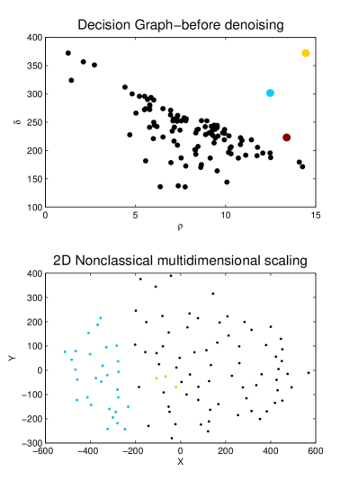
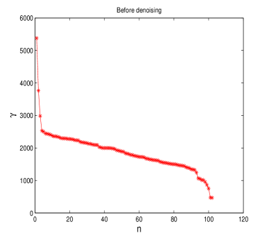
We do as the steps described above to cluster for the roads with velocity before and after denoising. From the decision graph, the first row in Figure 5, and the $\gamma$ variance in Figure 6, we should choose 3 clusters for the 102 roads both before and after denoising. In order to observe the performance of classification obviously, we calculate the 2 dimensional non-local multidimensional scaling matrix just as [47] does. This matrix with 2 columns is an approximation of the original distance matrix whose diagonal elements are all 0 and off-diagonal element in location $(i,j)$ represents the distance of road $i$ and $j$. The distance here refers to the $l^{2}$ norm of their velocity vectors’ difference. With the help of the approximated scaling matrix, we present the clustering result in the 2D non-local multidimensional scaling figure, the second row of Figure 5, where the X axis and Y axis represent the first and second column of this matrix correspondingly.

Figure 5: Decision graph and clustering result for the 102 roads.

Figure 6: $\gamma$ variance before and after denoising.

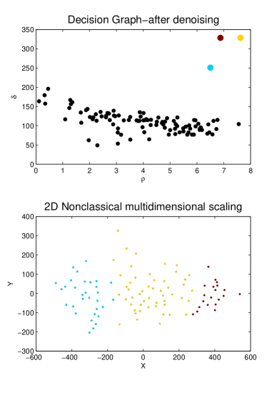
We illustrate the detailed result of clustering in the following. The 3 cluster centers are the color points in the first row of Figure 5. The other points are shown with the color consistent in the second row of Figure 5 and classified as follows:

• Before denoising, cluster 1 with 29 core elements and 0 halos corresponds to the blue points in the 2D non-local multidimensional scaling figure, and cluster 2 with 27 elements only has 3 core elements corresponding to the yellow points, and cluster 3 with 46 elements has no core elements. In the figure before denoising, if a point is a halo, then its color is black in the 2D non-local multidimensional scaling figure.

• After denoising, the three clusters all have no halos. Cluster 1 has 31 core points, 29 of which are exactly the ones that in cluster 1 before denoising, and cluster 3 has 20 core points. Roads belong to cluster 1,2,3 are represented by the blue, yellow and purple points respectively in the 2D non-local multidimensional scaling figure. As there are no halos after denoising, so no black points appear this time.

Now we give some further explanations on the clustering result. Note that roads in Beijing are divided into 6 types, which are urban express highway, freeway, national highway, provincial highway, prefectural highway and rural street, the corresponding type value is from 1 to 6 respectively. In order to illustrate more clearly, we list some related quantities after BV denoising in Table 3.

Table 3: Some Basic Properties of the 3 Clusters.

cluster	average velocity	average $\operatorname{TV}$	range	range
number	of cluster center	of cluster center	of velocity	of $\operatorname{TV}$
1	54.052	123.414	[46.165,65.398]	[56.544,259.974]
2	32.321	104.428	[21.967,48.021]	[95.165,482.275]
3	14.965	210.578	[6.396,20.641]	[118.177,239.608]

If a negative and positive linear transformation are made for average velocity and total variation respectively, then the trend of variables obtained is consistent with that of X and Y in the last one of Figure 5. Therefore, cluster 1 corresponds to roads with high average velocity and relatively low total variation. Namely, they should be matched with smaller road type value, meaning that most of them are urban express highway and freeway. In fact, there are 9 roads whose type value is 1, and 17 ways whose value is 2 in cluster 1. Cluster 3 contain roads with low average speed and bigger total variation, corresponding to prefectural highway or rural Street. It has been checked that all the roads’ type value are 6 in cluster 3 after denoising. And cluster 2 has the medial value in terms of average speed and total variation, indicating it can contain more types of roads, which is consistent with the fact there are 8 freeways, 15 provincial highways and 28 rural streets.

Figure 7: The clustering result matched with the original 102 roads. The horizontal axis represents longitude, and vertical axis represents latitude.

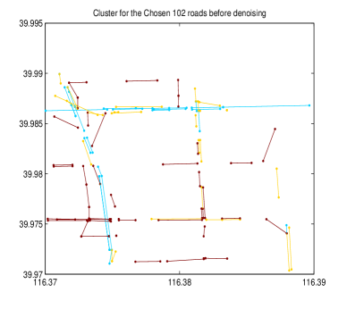
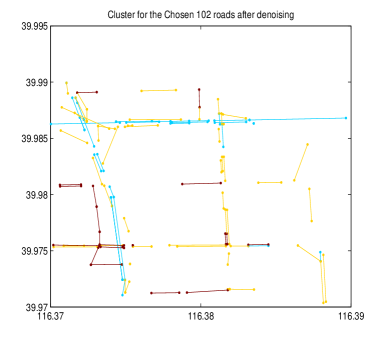
Finally, in order to observe the clustering result more directly, we match the 102 points above with the original 102 roads in corresponding colors and show them in Figure 7, where the horizontal axis represents longitude, and vertical axis means latitude. From Figure 7, we can see the clustering result improved greatly after denoising. There are 28 roads belonging to different clusters before and after denoising, and most of them are rural streets. This is consistent with our common sense. By BV denoising method, these roads are discovered and the noise part is eliminated.

From the clustering results, we see halos disappear with the BV denoising method. Because outliers often lie in halos, so we can say we obtain the clean data by denoising on the original velocity. This shows our denoising method works well.

4 Conclusions

In this paper, we applied the BV denoising method for urban traffic analysis by proposing easy-to-implement noise strength estimation algorithms. By applying the BV denoising method, we have showed the road velocity prediction accuracy is improved for real urban traffic data from Beijing Taxi GPS system. We have also verified that the road clustering based on velocity profile are improved significantly by applying the BV denoising method with best noise-strength estimate.

In this work, we considered only the temporal characteristics of road velocity profiles. In a follow-up study, we will consider both temporal and spatial characteristics, which will be more mathematically involved and is expected to give better results.

Appendix: Proof of Theorem 2.1.

In order to prove Theorem 2.1, we give a lemma first.

Lemma A.1.

Let $u_{0}(x_{i})=u_{i}+\xi_{i},i\in[N]$, where $u_{0}(x_{i})$, $u_{i}$, $\xi_{i}$ represent the observed, denoised data and noise for time slice $i$ separately. $u_{i}^{(j)},i\in[N_{j+1}],j=0,1,2$ are defined as in Theorem 2.1, and $v_{i}^{j},i\in[N_{j+1}],j=0,1,2$ are defined as in (9). Then the following relations hold:

$$\sum_{i=1}^{N_{2}}(u_{i}^{(1)}-v^{1}_{i})^{2} =\frac{1}{4}\sum_{i=1}^{N_{1}}(u_{i}-u_{0}(x_{i}))^{2}+\frac{1}{2}\sum_{i=1}^{N_{2}}(u_{2i-1}-u_{0}(x_{2i-1}))(u_{2i}-u_{0}(x_{2i})),$$

$$\sum_{i=1}^{N_{3}}(u_{i}^{(2)}-v^{2}_{i})^{2} =\frac{1}{4}\sum_{i=1}^{N_{2}}(u_{i}^{(1)}-v^{1}_{i})^{2}+\frac{1}{2}\sum_{i=1}^{N_{3}}(u_{2i-1}^{(1)}-v^{1}_{2i-1})(u^{(1)}_{2i}-v^{1}_{2i}).$$

Proof A.2 (Proof of Lemma A.1).

1) For the first equation, let $h_{2}=2h$, we have

$$\sum_{i=1}^{N_{2}}(u_{i}^{(1)}-v^{1}_{i})^{2}\cdot h_{2} =\sum_{i=1}^{N_{2}}(\frac{u_{2i}+u_{2i-1}}{2}-\frac{u_{0}(x_{2i})+u_{0}(x_{2i-1})}{2})^{2}\cdot 2h$$

$$=\sum_{i=1}^{N_{2}}(\frac{u_{2i}-u_{0}(x_{2i})}{2}+\frac{u_{2i-1}-u_{0}(x_{2i-1})}{2})^{2}\cdot 2h$$

$$=\frac{h}{2}\sum_{i=1}^{N_{1}}(u_{i}-u_{0}(x_{i}))^{2}+h\sum_{i=1}^{N_{2}}(u_{2i}-u_{0}(x_{2i}))(u_{2i-1}-u_{0}(x_{2i-1}))$$

Rearrange the equation above and then the formula for $\sum_{i=1}^{N_{2}}(u_{i}^{(1)}-v^{1}_{i})^{2}$ is obtained.

2) For the second equation, let $h_{3}=4h$, the proof can be done with similar procedure. ∎

Proof A.3 (Proof of Theorem 2.1).

We prove this theorem in three steps.
(1) By definition of $V_{1}$, we get

$$V_{1}=\frac{1}{h}(2\sum_{i=1}^{N_{1}}(u_{0}(x_{i}))^{2}-(u_{0}(x_{1}))^{2}-(u_{0}(x_{N_{1}}))^{2}-2\sum_{i=1}^{N_{1}-1}u_{0}(x_{i})u_{0}(x_{i+1})).$$

By using the representation of $\sum_{i=1}^{N_{1}}(u_{0}(x_{i}))^{2}$ from equation (7), we get

$$V_{1}=\frac{4\sigma^{2}}{h^{2}}+\frac{1}{h}(4\sum_{i=1}^{N_{1}}u_{i}u_{0}(x_{i})-2\sum_{i=1}^{N_{1}}(u_{i})^{2}-(u_{0}(x_{1}))^{2}-(u_{0}(x_{N_{1}}))^{2}-2\sum_{i=1}^{N_{1}-1}u_{0}(x_{i})u_{0}(x_{i+1})).$$

Similarly, combine the definition of $V_{2}$, $V_{3}$ and Lemma A.1, we obtain the representation of $V_{2}$ and $V_{3}$

$$V_{2} =\frac{\sigma^{2}}{2h^{2}}+\frac{1}{2h}\Big{(}\sum_{i=1}^{N_{2}}(u_{2i-1}-u_{0}(x_{2i-1}))(u_{2i}-u_{0}(x_{2i}))$$

$$\quad+4\sum_{i=1}^{N_{2}}u_{i}^{(1)}v^{1}_{i}-2\sum_{i=1}^{N_{2}}(u_{i}^{(1)})^{2}-(v^{1}_{1})^{2}-(v^{1}_{N_{2}})^{2}-2\sum_{i=1}^{N_{2}-1}v^{1}_{i}v^{1}_{i+1}\Big{)},$$

$$V_{3} =\frac{\sigma^{2}}{16h^{2}}+\frac{1}{4h}\Big{(}\frac{1}{4}\sum_{i=1}^{N_{2}}(u_{2i-1}-u_{0}(x_{2i-1}))(u_{2i}-u_{0}(x_{2i}))+\sum_{i=1}^{N_{3}}(u^{(1)}_{2i-1}-v^{1}_{2i-1})(u_{2i}^{(1)}-v^{1}_{2i})$$

$$\quad+4\sum_{i=1}^{N_{3}}u_{i}^{(2)}v^{2}_{i}-2\sum_{i=1}^{N_{3}}(u_{i}^{(2)})^{2}-(v^{2}_{1})^{2}-(v^{2}_{N_{3}})^{2}-2\sum_{i=1}^{N_{3}-1}v^{2}_{i}v^{2}_{i+1}\Big{)}.$$

(2) Now, we are ready to apply the assumptions in the theorem.
After regrouping the order of the representation of $V_{1},V_{2},V_{3}$ and replacing $u_{0}(x_{i})$ with $u_{i}+\xi_{i}$, we obtain

$$V_{1} =\frac{2}{h}\sum_{i=1}^{N_{1}-1}((u_{i+1}-u_{i})(\xi_{i+1}-\xi_{i})-\xi_{i}\xi_{i+1})+\frac{4\sigma^{2}}{h^{2}}-\frac{\xi_{1}^{2}}{h}-\frac{\xi_{N_{1}}^{2}}{h}+\sum_{i=1}^{N_{1}-1}(u_{i}-u_{i+1})^{2}\frac{1}{h},$$

$$V_{2} =\frac{\sigma^{2}}{2h^{2}}+\frac{1}{2h}(\sum_{i=1}^{N_{2}}\xi_{2i-1}\xi_{2i}-(\frac{\xi_{1}+\xi_{2}}{2})^{2}-(\frac{\xi_{N_{1}-1}+\xi_{N_{1}}}{2})^{2}$$

$$\quad+\sum_{i=1}^{N_{2}-1}((u_{i+1}^{(1)}-u_{i}^{(1)})(\xi_{2i+1}+\xi_{2i+2}-\xi_{2i-1}-\xi_{2i})-\frac{(\xi_{2i-1}+\xi_{2i})(\xi_{2i+1}+\xi_{2i+2})}{2})+\sum_{i=1}^{N_{2}-1}(u_{i+1}^{(1)}-u_{i}^{(1)})^{2}),$$

$$V_{3} =\frac{\sigma^{2}}{16h^{2}}+\frac{1}{4h}(\frac{1}{4}\sum_{i=1}^{N_{2}}\xi_{2i-1}\xi_{2i}+\sum_{i=1}^{N_{3}}\frac{(\xi_{4i-3}+\xi_{4i-2})(\xi_{4i-1}+\xi_{4i})}{4}-\frac{(\sum_{i=1}^{4}\xi_{i})^{2}+(\sum_{j=0}^{3}\xi_{N_{1}-j})^{2}}{16}$$

$$\quad+\sum_{i=1}^{N_{3}-1}(u_{i}^{(2)}-u_{i+1}^{(2)})^{2}+\sum_{i=1}^{N_{3}-1}(\frac{(u_{i+1}^{2}-u_{i}^{(2)})(\sum_{j=1}^{4}(\xi_{4i+j}-\xi_{4i+1-j}))}{2}-\frac{(\sum_{j=0}^{3}\xi_{4i-j})(\sum_{j=1}^{4}\xi_{4i+j})}{8})).$$

Take expectation on the equations above and combine the assumptions, then

$$\mathbb{E}(V_{1}) =(4-\frac{4}{N})\frac{\sigma^{2}}{h^{2}}+\sum_{i=1}^{N_{1}-1}(u_{i+1}-u_{i})^{2}\cdot\frac{1}{h},$$

$$\mathbb{E}(V_{2}) =(\frac{1}{2}-\frac{1}{N})\frac{\sigma^{2}}{h^{2}}+\sum_{i=1}^{N_{2}-1}(u_{i+1}^{(1)}-u_{i}^{(1)})^{2}\cdot\frac{1}{2h},$$

$$\mathbb{E}(V_{3}) =(\frac{1}{16}-\frac{1}{4N})\frac{\sigma^{2}}{h^{2}}+\sum_{i=1}^{N_{3}-1}(u_{i+1}^{(2)}-u_{i}^{(2)})^{2}\cdot\frac{1}{4h}.$$

From what have done above, we can estimate $\sigma$ by fitting a line with 3 points: $(4-\frac{4}{N},V_{1}),(\frac{1}{2}-\frac{1}{N},V_{2}),(\frac{1}{16}-\frac{1}{4N},V_{3})$. The slope of the line is $\frac{\sigma^{2}}{h^{2}}$, then $\sigma$ is estimated.
(3) Estimate the value of $\sigma$. Set

$$X_{1}=4-\frac{4}{N},\quad X_{2}=\frac{1}{2}-\frac{1}{N},\quad X_{3}=\frac{1}{16}-\frac{1}{4N},$$

and assume $(X_{1},V_{1}),(X_{2},V_{2}),(X_{3},V_{3})$ satisfy

$$V_{i}=AX_{i}+b+\mu_{i},\quad i=1,2,3,$$

where $\mu_{i}$ stand for some small random disturbance variables.
Then we want to fit a line with these 3 points, which is

$$V=\hat{A}X+\hat{b}.$$

With the help of least square method, we obtain the representation of $\hat{A}$ as follows:

$$\hat{A}=\frac{3\sum_{i=1}^{3}X_{i}V_{i}-\sum_{i=1}^{3}X_{i}\sum_{i=1}^{3}V_{i}}{3\sum_{i=1}^{3}X_{i}^{2}-(\sum_{i=1}^{3}X_{i})^{2}}.$$ (13)

So we estimate $\sigma^{2}$ by

$$\hat{\sigma}^{2}=h^{2}\frac{(\frac{119}{16}-\frac{27}{4N})V_{1}+(\frac{9}{4N}-\frac{49}{16})V_{2}+(\frac{9}{2N}-\frac{35}{8})V_{3}}{\frac{3577}{128}+\frac{189}{8N^{2}}-\frac{819}{16N}}.$$

Combine the assumption $V_{i}=AX_{i}+b+\mu_{i},i=1,2,3,$ and (13), we get

$$\hat{A}=A+\frac{3\sum_{i=1}^{3}X_{i}\mu_{i}-\sum_{i=1}^{3}X_{i}\sum_{i=1}^{3}\mu_{i}}{3\sum_{i=1}^{3}X_{i}^{2}-(\sum_{i=1}^{3}X_{i})^{2}}.$$ (14)

Thus,

$$\mathbb{E}(\hat{A})=A+\frac{3\sum_{i=1}^{3}X_{i}\mathbb{E}(\mu_{i})-\sum_{i=1}^{3}X_{i}\sum_{i=1}^{3}\mathbb{E}(\mu_{i})}{3\sum_{i=1}^{3}X_{i}^{2}-(\sum_{i=1}^{3}X_{i})^{2}}.$$ (15)

Notice that by the construct of $V_{i}$ and the linear assumption for $V_{i},i=1,2,3$, the following relations are established:

$$b+\mu_{1}=\sum_{i=1}^{N_{1}-1}|u_{i+1}-u_{i}|^{2}\cdot\frac{1}{h}=V_{1}^{c},$$

$$b+\mu_{2}=\sum_{i=1}^{N_{2}-1}|u^{(1)}_{i+1}-u^{(1)}_{i}|^{2}\cdot\frac{1}{2h}=V_{2}^{c},$$

$$b+\mu_{3}=\sum_{i=1}^{N_{3}-1}|u^{(2)}_{i+1}-u^{(2)}_{i}|^{2}\cdot\frac{1}{4h}=V_{3}^{c}.$$

Substitute $\mathbb{E}(\mu_{i})=V_{i}^{c}-b$ into (15), we derive

$$\mathbb{E}(\hat{A})=A+\frac{(\frac{49}{16}-\frac{9}{4N})(V_{1}^{c}-V_{2}^{c})+(\frac{35}{8}-\frac{9}{2N})(V_{1}^{c}-V_{3}^{c})}{\frac{3577}{128}+\frac{189}{8N^{2}}-\frac{819}{16N}}.$$

Denote

$$Bias(N)=h^{2}\frac{(\frac{49}{16}-\frac{9}{4N})(V_{1}^{c}-V_{2}^{c})+(\frac{35}{8}-\frac{9}{2N})(V_{1}^{c}-V_{3}^{c})}{\frac{3577}{128}+\frac{189}{8N^{2}}-\frac{819}{16N}}.$$ (16)

Because $\hat{A}=\frac{\hat{\sigma}^{2}}{h^{2}}$, $A=\frac{\sigma^{2}}{h^{2}}$, we get equation (11). ∎

References

- [1] W. Liu, Y. Zheng, S. Chawla, J. Yuan, and X. Xing, Discovering spatio-temporal causal interactions in traffic data streams, in ACM SIGKDD International Conference on Knowledge Discovery and Data Mining, pp. 1010–1018 (2011).
- [2] Z. Wang, M. Lu, X. Yuan, J. Zhang, and H. V. D. Wetering, Visual traffic jam analysis based on trajectory data, IEEE Transactions on Visualization Computer Graphics, 19(12), pp. 2159–2168 (2013).
- [3] J. Yuan, Y. Zheng, C. Zhang, W. Xie, X. Xie, G. Sun, and Y. Huang, T-drive: driving directions based on taxi trajectories, in SIGSPATIAL International Conference on Advances in Geographic Information Systems, pp. 99–108 (2010).
- [4] J. Kim and H. S. Mahmassani, Spatial and temporal characterization of travel Patterns in a Traffic Network Using Vehicle Trajectories, Transportation Research Part C: Emerging Technologies, 59, pp. 375–390 (2015).
- [5] A. T. Palma, V. Bogorny, B. Kuijpers, and L. O. Alvares, A clustering-based approach for discovering interesting places in trajectories, in ACM Symposium on Applied Computing, pp. 863–868 (2008).
- [6] X. Zhan, Y. Zheng, X. Yi, and S. Ukkusuri, Citywide Traffic Volume Estimation Using Trajectory Data, IEEE Transactions on Knowledge Data Engineering, 29(2), pp. 272–285 (2017).
- [7] A. D. Brébisson, E. Simon, A. Auvolat, P. Vincent, and Y. Bengio, Artificial neural networks applied to taxi destination prediction, in Proceedings of the 2015 International Conference on ECML PKDD Discovery Challenge 1526 pp. 40–51 (2015).
- [8] N. Sadek and A. Khotanzad, Multi-scale high-speed network traffic prediction using -factor Gegenbauer ARMA model, in IEEE International Conference on Communications, 4 pp. 2148–2152 (2004).
- [9] W. Min and L. Wynter, Real-time road traffic prediction with spatio-temporal correlations, Transportation Research Part C: Emerging Technologies, 19(4), pp. 606–616 (2011).
- [10] Y. Zhu, Z. Li, H. Zhu, M. Li, and Q. Zhang, A compressive sensing approach to urban traffic estimation with probe vehicles, IEEE Transactions on Mobile Computing, 12(11), pp. 2289–2302 (2013).
- [11] H. Xiao, H. Sun, and B. Ran, Fuzzy-neural network traffic prediction framework with wavelet decomposition, Transportation Research Record Journal of the Transportation Research Board, 1836(1), pp.16–20 (2003).
- [12] Z. Zheng and D. Su, Traffic state estimation through compressed sensing and Markov random field, Transportation Research Part B Methodological, 91 pp. 525–554 (2016).
- [13] D. Yarotsky, Error bounds for approximations with deep ReLU networks, Neural Networks, 94, pp. 103–114 (2017).
- [14] S. Liang and R. Srikant, Why deep neural networks for function approximation?, arXiv:1610.04161, 2017.
- [15] Y. Tang and C. Eliasmith, Deep networks for robust visual recognition, in Proceedings of the 27th International Conference on Machine Learning, pp. 1055–1062 (2010).
- [16] S. J. Nowlan and G. E. Hinton, Simplifying neural networks by soft weight-sharing, Neural computation, 4(4), pp. 473–493 (1992).
- [17] P. Vincent, H. Larochelle, Y. Bengio, and P.-A. Manzagol, Extracting and composing robust features with denoising autoencoders, in Proceedings of the 25th International Conference on Machine Learning, ACM, pp. 1096–1103 (2008).
- [18] P. Vincent, H. Larochelle, I. Lajoie, Y. Bengio, and P.-A. Manzagol, Stacked denoising autoencoders: Learning useful representations in a deep network with a local denoising criterion, Journal of Machine Learning Research, 11, pp. 3371–3408 (2010).
- [19] L. Maaten, M. Chen, S. Tyree, and K. Weinberger, Learning with marginalized corrupted features, in International Conference on Machine Learning, pp. 410–418 (2013).
- [20] N. Srivastava, G. Hinton, A. Krizhevsky, I. Sutskever, and R. Salakhutdinov, Dropout: a simple way to prevent neural networks from overfitting, The Journal of Machine Learning Research, 15(1), pp. 1929–1958 (2014).
- [21] L. I. Rudin, S. Osher, and E. Fatemi, Nonlinear total variation based noise removal algorithms, Physica D: Nonlinear Phenomena, 60(1), pp. 259–268 (1992).
- [22] Y.-L. You and M. Kaveh, Fourth-order partial differential equations for noise removal, IEEE Trans. Image Process., 9(10), pp. 1723–1730, (2000).
- [23] M. Mahmoudi and G. Sapiro, Fast image and video denoising via nonlocal means of similar neighborhoods, IEEE Signal Processing Letters, 12(12), pp. 839–842 (2005).
- [24] P. Bao and X. Ma, Image adaptive watermarking using wavelet domain singular value decomposition, IEEE Transactions on Circuits and Systems for Video Technology, 15(1), pp. 96–102 (2005).
- [25] R. G. Baraniuk, Compressive sensing, IEEE Signal Processing Magazine, 24(4), pp. 118–121 (2007).
- [26] W. Yin, S. Osher, D. Goldfarb, and J. Darbon, Bregman iterative algorithms for -minimization with applications to compressed sensing, SIAM J. Imaging Sci., 1(1), pp. 143–168 (2008).
- [27] K. Dabov, A. Foi, and K. Egiazarian, Video denoising by sparse 3d transform-domain collaborative filtering, in Signal Processing Conference, 2007 European, pp. 145–149 (2008).
- [28] J. Cai, S. Osher, and Z. Shen, Split bregman methods and frame based image restoration, Multiscale Model. Simul., 8(2), pp. 337–369 (2009).
- [29] C. Wu and X. Tai, Augmented Lagrangian method, dual methods, and split Bregman iteration for ROF, vectorial TV, and high order models, SIAM J. Imaging Sci., 3(3), pp. 300–339 (2010).
- [30] C. Liu and W. T. Freeman, A High-Quality Video Denoising Algorithm Based on Reliable Motion Estimation, in European Conference on Computer Vision (2010).
- [31] H. Ji, C. Liu, Z. Shen, and Y. Xu, Robust video denoising using low rank matrix completion, in Computer Vision and Pattern Recognition, pp. 1791–1798 (2010).
- [32] Z.-F. Pang, L.-L. Wang, and Y.-F. Yang, Fast algorithms for the anisotropic LLT model in image denoising, East Asian J. Appl. Math., 1(3), pp. 264–283 (2011).
- [33] B. Shi, Z.-F. Pang, and Y.-F. Yang, A projection method based on the splitting Bregman iteration for the image denoising, J. Appl. Math. Comput., 39(1), pp. 533–550 (2012).
- [34] X. Zhang, Y. Shi, Z.-F. Pang, and Y. Zhu, Fast algorithm for image denoising with different boundary conditions, Journal of the Franklin Institute, 354(11), pp. 4595–4614 (2017).
- [35] W. Yang, Z. Huang, and W. Zhu, An efficient tailored finite point method for Rician denoising and deblurring, Commun Comput Phys, 24 pp. 1169-1195 (2018).
- [36] T. Wei, L. Wang, P. Lin, J. Chen, Y. Wang, and H. Zheng, Learning non-negativity constrained variation for image denoising and deblurring, Numerical Mathematics: Theory, Methods and Applications, 10(4), pp. 852–871 (2017).
- [37] F. Sciacchitano, Y. Dong, and M. S. Andersen, Total variation based parameter-free model for impulse noise removal, Numerical Mathematics: Theory, Methods and Applications, 10(1), pp. 186–204 (2017).
- [38] D. Jiang, X. Wang, G. Xu, and J. Lin, A denoising-decomposition model combining TV minimisation and fractional derivatives, East Asian Journal on Applied Mathematics, 8(3), pp. 447–462 (2018).
- [39] Z. Zheng, S. Ahn, D. Chen, and J. Laval, Applications of wavelet transform for analysis of freeway traffic: Bottlenecks, transient traffic, and traffic oscillations, Transportation Research Part B Methodological, 45(2), pp. 372–384 (2011).
- [40] D. W. Xu, H. H. Dong, H. J. Li, L. M. Jia, and Y. J. Feng, The estimation of road traffic states based on compressive sensing, Transportmetrica B:Transport Dynamics, 3(2), pp. 131–152 (2015).
- [41] D. Strong and T. Chan, Edge-preserving and scale-dependent properties of total variation regularization, Inverse Problems, 19(6), pp. 165–187 (2003).
- [42] J. B. Rosen, The Gradient Projection Method for Nonlinear Programming. Part I. Linear Constraints, Journal of the Society for Industrial Applied Mathematics, 9(4), pp. 514–532 (1961).
- [43] A. Chambolle, V. Caselles, M. Novaga, D. Cremers, and T. Pock, An introduction to total variation for image analysis, in Radon Series Comp. Appl. Math, 9, pp. 263–340 (2010).
- [44] C. Wu, J. Zhang, and X.-C. Tai, Augmented Lagrangian method for total variation restoration with non-quadratic fidelity, Inverse Probl. Imaging, 5(1), pp. 237–261 (2011).
- [45] E. J. Candès and B. Recht, Exact Matrix Completion via Convex Optimization, Foundations of Computational Mathematics, 9, pp. 717 (2009).
- [46] M. Fazel, H. Hindi, and S. P. Boyd, A rank minimization heuristic with application to minimum order system approximation, in Proceedings of the American Control Conference, 6, pp. 4734–4739 (2001).
- [47] A. Rodriguez and A. Laio, Clustering by fast search and find of density peaks, Science, 344(6191), p. 1492 (2014).
- [48] H. Xiong, G. Pandey, M. Steinbach, and V. Kumar, Enhancing data analysis with noise removal, IEEE Transactions on Knowledge Data Engineering, 18(3), pp. 304–319 (2006).
- [49] Y. Liu, Z. Li, H. Xiong, X. Gao, and J. Wu, Understanding of internal clustering validation measures, in IEEE 10th International Conference on Data Mining (ICDM), pp. 911–916 (2010).