revtex4-1Repair the float pdftexdestination with the same figuret

Critical fluctuations and slowing down of chaos

Abstract

Fluids cooled to the liquid-vapor critical point develop system-spanning fluctuations in density that transform their visual appearance. Despite the rich phenomenology of this critical point, there is not currently an explanation of the underlying mechanical instability. How do structural correlations in molecular positions overcome the destabilizing force of deterministic chaos in the molecular dynamics? Here, we couple techniques from nonlinear dynamics and statistical physics to analyze the emergence of this singular state. Our numerical simulations reveal that the ordering mechanisms of critical dynamics are directly measurable through the hierarchy of spatiotemporal Lyapunov modes. A subset of unstable modes softens near the critical point, with a marked suppression in their characteristic exponents reflecting a weakened sensitivity to initial conditions. Finite-time fluctuations in these exponents, however, exhibit diverging dynamical timescales and power law signatures of critical dynamics. Collectively, these results are symptomatic of a critical slowing down of chaos that sits at the root of our statistical understanding of the singular thermodynamic responses at the liquid-vapor critical point.

Fluctuations are sovereign in critical phenomena Stanley (1988); *Goldenfeld92. Fluids at the liquid-vapor critical point are not immune. These critical points Smoluchowski (1908) are unique instabilities that punctuate the space of thermodynamic states. First established experimentally by Andrews Andrews (1869), the liquid-gas critical point was given a molecular explanation shortly thereafter by van der Waals Sengers (2002). Van der Waals’ picture, now a paradigm in liquid state theory Hansen and McDonald (1986); *Barrat03, is that the repulsive forces largely determine the structural arrangements of molecules in non-critical liquids, not the attractive forces. Near the liquid-vapor critical point, however, their roles reverse and the paradigm shifts Widom (1967); dynamical fluctuations reach macroscopic magnitude and overrule molecular size, shape, and interactions in dictating bulk behavior. These fluctuations are generated by the deeply nonlinear dynamics of classical, critical fluids. Yet, the relationship between microscopic dynamical instability and the thermodynamic singularity has never been entirely clear Berry et al. (2000).

While the field of critical phenomena continues to absorb increasingly diverse systems Nielsen et al. (2000), the basic phenomenology is firmly established Stanley (1988); *Goldenfeld92. Its taxonomy is built on scaling and universality, the similar behavior of dissimilar systems. Despite the early discovery of their critical points, fluids were somewhat resistant to classification Sengers (2002). Simulations Simeoni et al. (2010) and theory Poland and Simmons-Duffin (2016) were, and continue to be, integral in providing mechanistic insights, the location of the critical point, and estimates of static critical exponents Johnson et al. (1993); Caillol (1998); Potoff and Panagiotopoulos (1998); Watanabe et al. (2012). Through simulations, the classical atomistic dynamics of fluids are also known to be chaotic Bosetti and Posch (2014), which is measurable through the machinery of nonlinear dynamics. Nonlinear dynamics, which includes the notion of deterministic chaos in its repertoire, has given insight into the physical mechanisms of the jamming transition in granular materials Banigan et al. (2013), self-organizing systems Green et al. (2013), evaporating collections of nuclei Colonna and Bonasera (1999); Bonasera et al. (1995), and the phase changes of atomic clusters Amitrano and Berry (1992); *WalesB94; *CalvoL98; *Calvo10. Recently, the dynamics of model spatially-extended systems have been assigned to known dynamic universality classes Pazó et al. (2016, 2013). But, the dynamic scaling of chaos in fluids near thermodynamic critical points has not yet been explored. The recent steps to further coalesce statistical physics and nonlinear dynamics reinvigorate the question of how fluids, specifically their atomistic dynamics, fit within the phenomenological architecture of critical phenomena.

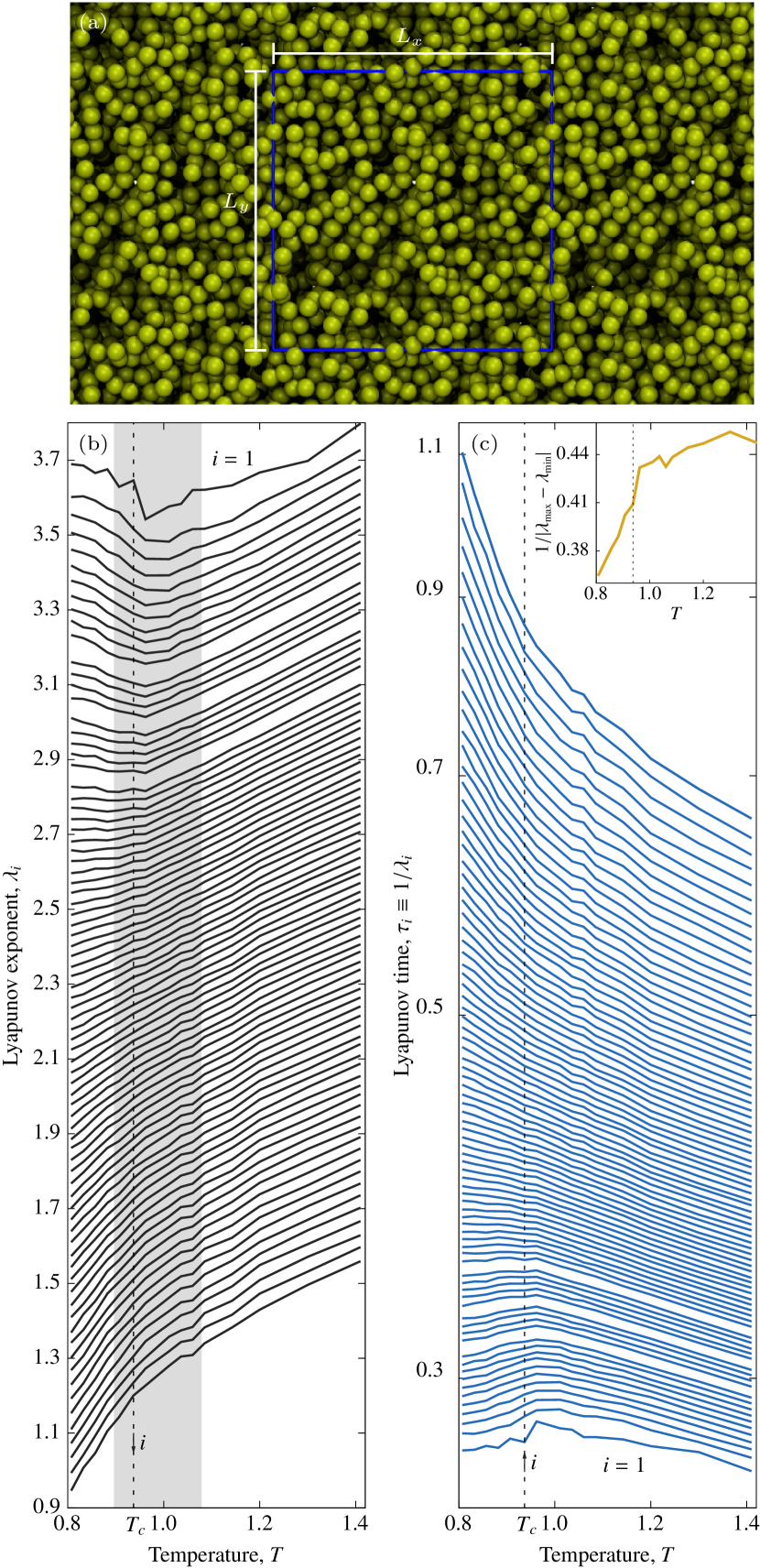
Figure 1: Slowing down the divergence of trajectories at the liquid-vapor critical point. (a) Snapshot of the critical fluid and the periodic boundaries of length $L=L_{x}=L_{y}=L_{z}$. (b) Spectra of Lyapunov exponents $\lambda_{i}$ and (c) Lyapunov times $\tau_{i}$ (log-linear scale) as a function of the mean kinetic temperature, $T$. Every 30 $\lambda_{i}$ are shown for $N=1000$ particles occupying a cubic simulation volume with a density $\rho=\rho_{c}=0.317$. Unstable spatiotemporal modes that are more disordered ($1/3N\leq i/3N\leq 0.18$) have positive Lyapunov exponents (time) with a minimum (maximum) in the supercritical region. Vertical dashed lines mark the critical temperature, $T_{c}$. Inset illustrates compression of spectrum through the critical point for data shown.

At critical points, correlations span molecular-scale interactions to the entire system. These correlations imply structural organization that is intrinsically opposed by the chaotic dynamics. The mechanisms balancing this internal tension between order and instability, however, are subtle. As a result, theoretical explanations for the mechanical origins of critical phenomena are uncommon. Continuous transitions in crystals are a notable exception where structural changes arise through the instability of a lattice vibration Berry et al. (2000). There, the mode responsible for the phase transition is a collective excitation whose frequency decreases anomalously during an approach to the transition point. For example, in SrTiO₃ the frequency of a soft phonon mode decreases substantially and, ultimately, freezes at the transition temperature when approached from below Scott (1974). Because of the absence of long-range order in fluids – and an inability to make a small vibration approximation, as in solids, or a molecular randomness hypothesis, as in gases Landau and Lifshitz (1958) – the dynamical instability in critical fluids has been grounded in purely statistical terms.

To analyze the instability of the liquid-vapor critical point, we apply nonlinear dynamical techniques to molecular simulations of a homogeneous, single-component, non-associated fluid. The system we simulate, shown in Fig. 1(a), consists of $N$ particles interacting pairwise through van der Waals forces, repelling (attracting) at distances of a (few) molecular diameter(s) according to the Lennard-Jones potential Jones (1924). It has a critical point, a triple point, and three phases (solid, liquid, and gas) that are independently identifiable through a variety of molecular simulation techniques Allen and Tildesley (1987); Frenkel and Smit (2001) and is generally considered to belong to the Ising universality class Caillol (1998); Watanabe et al. (2012). We use the hierarchy of $6N$ spatiotemporal modes, Lyapunov vectors, as order parameters. Each mode has an associated exponent, $\lambda_{i}$ indexed $i=1,\ldots,6N$ Pikovsky and Politi (2016) and in descending order, that measures the contribution of each mode to the global dynamics. Each $\lambda_{i}$ is the average of the $i$-th finite-time Lyapunov exponent $\lambda_{i}(t)$ over $10^{4}$ trajectories. Larger exponents indicate more unstable, collective modes Tailleur and Kurchan (2007). In our simulations at fixed number of particles $N$, energy $E$, and volume $V$, we calculate the full Lyapunov spectrum at the critical density $\rho_{c}$ and over a range of temperatures including the critical temperature. We choose the energy density to fix the mean kinetic temperature, $T$ (Methods).

The critical point as a limit of dynamical order in unstable Lyapunov modes.– When approaching the liquid-vapor critical point from above, $T>T_{c}$, spatial regions form that will become vapor and liquid after the system is cooled to $T<T_{c}$ through the critical point $T_{c}$. The statistical correlations in these regions are also apparent in the Lyapunov modes, a set of dynamic vectors representing collective changes to molecular positions and momenta, Fig. 1 Gaspard (1998); Pikovsky and Politi (2016). For example, the magnitude of the largest Lyapunov exponent, $\lambda_{1}$, is dominated by the fastest dynamical events in the system Posch and Forster (2005). In simple fluids, the fastest events are pairwise interactions sampling the repulsive part of the potential Das et al. (2017). As shown in Fig. 1(b), there is a minimum in the largest Lyapunov exponent near the known Errington and Debenedetti (2003) critical point, ($T_{c},\rho_{c}$), giving direct evidence that critical conditions inhibit the effect of repulsive forces on the dynamics. Compared to the coexistence, $T<T_{c}$, or supercritical regimes, $T>T_{c}$, the minimum in this exponent and the maximum in the Lyapunov time, $1/\lambda_{1}$ in Fig. 1(c), also means the critical dynamics are predictable over longer timescales because initially similar configurations do not diverge as quickly. That is, the statistical correlations typically invoked to explain this critical phenomenon are a reflection of the slowing down of chaos and suppressed instability in critical dynamics.

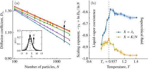
Figure 2: Finite-size scaling of fluctuations in dynamical observables. (a) Fluctuations in the kinetic energy and Lyapunov exponents decay with increasing number of particles (log-log): the diffusion coefficients follow a power law $D_{\scriptsize{X}}(N,T)\sim N^{-\gamma_{\scriptsize{X}}(T)}$ for $11$ system sizes from $N=100$ to $2000$. The corresponding probability distributions also concentrate (Inset: first Lyapunov exponent at $\rho=\rho_{c}=0.317$ and $T=T_{c}=0.937$) (b) The wandering exponents, $\gamma_{\scriptsize{X}}(T)$, of the first finite-time Lyapunov exponent and the kinetic energy per particle, $K/N$, peak at the critical temperature, $T_{c}$, at the critical density $\rho=\rho_{c}$. Error bars indicate standard error ($1\,\sigma$) for parameter estimates from linear fits in (a).

The minimum in the first Lyapunov exponent signals the breakdown of the van der Waals picture, from which statistical mechanical treatments of liquids are typically built Widom (1967). These perturbative treatments assume the structure of a dense, monatomic liquid resembles that of a hard sphere fluid and, to a first approximation, the attractive interactions have little effect on the liquid structure Barrat and Hansen (1988). However, this picture does not hold near the critical point, and repulsive intermolecular forces instead play a subordinate role compared to critical fluctuations as we see through the suppression of the first Lyapunov exponent. This finding differs from the jamming transition in granular materials, though, which seems to be a transition from a chaotic to a non-chaotic state Banigan et al. (2013). The data in Fig. 1 suggests the continuous liquid-vapor phase transition remains chaotic throughout and into the coexistence region for finite-size systems.

To more fully resolve dynamical instability across the critical point, we measure the full spectrum of Lyapunov exponents. There are $3N$ positive exponents over the range of temperatures, suggesting the dynamics are chaotic (Methods). The shape of the spectrum depends sensitively on kinetic temperature and density Dellago and Posch (1996); Yang and Radons (2005); Das et al. (2017). Fig. 1(b) shows the spectrum at the critical density for temperatures spanning the critical temperature, $T_{c}$. The exponents of all unstable modes decrease when approaching the critical point from above. But, only the most unstable modes have exponents with minima at the critical point. Critical correlations appear to have the largest impact on the modes with scaled index up to $i/3N\approx 0.18$. Exponents beyond this point increase monotonically with temperature. The spectrum is also compressed at the critical point, Fig. 1(c) inset, meaning there is a weaker preference for trajectories to diverge in the direction of any given mode.

Overall, these spectra show that critical dynamics are less sensitive to the detailed features of intermolecular forces but also initial conditions. Because the Lyapunov modes are mechanical objects, with their own equations of motion, their associated spectra are direct evidence that these spatiotemporal modes resolve the mechanical instability generating the liquid-vapor critical point. Through these observables, critical conditions appear to constrain the dynamics so that different phase space directions have a homogeneous degree of instability relative to the supercritical $T>T_{c}$ or liquid-vapor coexistence $T<T_{c}$ regimes.

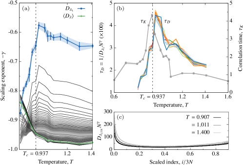
Figure 3: Critical slowing down of dynamical time scales of Lyapunov exponent fluctuations. Self-averaging and statistical dependence of spatial domains for the first exponent and the bulk near the critical point. (a) The (negative) wandering exponent as a function of temperature $T$ at $\rho_{c}$ for the diffusion coefficient of the first finite-time Lyapunov exponent. Also shown are the $-\gamma$ for average diffusion coefficients where averaging includes an increasing number of Lyapunov exponents in the spectrum. (b) Peak in the dynamical timescale for Lyapunov exponent fluctuations, $\tau_{D}\equiv 1/D_{\lambda_{1}}N^{\gamma}$, and peak in the correlation time of kinetic energy per particle, $\tau_{K}$. (c) Data collapse for the scaled diffusion coefficient of finite-time Lyapunov exponent spectra as a function of the scaled spectral indices: the functional form is the scaling function $\tilde{D}(T,\rho=\rho_{c})$. All data are at the critical density for the three-dimensional Lennard-Jones fluid.

Scaling relations and diverging timescales in fluctuations.– Cooling the fluid towards the critical point causes the correlation length to diverge. In our simulations, though, the correlation length saturates at the size of our simulation cell, $L$. Fleeting clusters of all sizes up to $L$, which will eventually become liquid, begin to appear. These clusters’ ephemeral existence clearly suppresses chaos in the critical dynamics on long timescales. However, their structure is only the spatial component of the mechanical system. The Lyapunov modes, though, are local directions in position and momentum. As the system structure evolves, the dynamics continues to temporarily sample phase space domains where trajectories diverge more quickly and more slowly than the average, domains that contribute significantly to the Lyapunov modes and the finite-time estimates of the Lyapunov exponents. Distributions of $\lambda_{1}(t)$ are shown in Fig. 2(a).

Power laws are a hallmark of critical phenomena Callen (1985) that quantify the divergence of a system’s response to small changes in external fields such as temperature. Non-trivial Aharony and Harris (1996) power law behavior is apparent in the decay of temporal Lyapunov exponent fluctuations with system size. At thermodynamic equilibrium, the precise scaling of relative fluctuations, termed self-averaging Milchev et al. (1986), in an observable $X$ decay according to $R_{X}=\left<\Delta X^{2}\right>/\left<X\right>^{2}\sim D_{\scriptsize{X}}/\left<X\right>^{2}\sim N^{-\gamma}$ with $\Delta X=X-\left<X\right>$, the wandering exponent $\gamma$, and a generalized diffusion coefficient $D_{\scriptsize{X}}$ (SI Sec. III). Loosely speaking, a system is self-averaging with respect to a given property $X$ if the value of the thermodynamic observable corresponds to the average over independent subsystems or, in this case, time windows. More precisely, the relative variance $R_{X}$ of the property $X$ vanishes in the thermodynamic limit: $R_{X}\to 0$ when $N\to\infty$. The wandering exponent $\gamma$ can have values between $0$ and $1$ – a value of one meaning the observable is strongly self-averaging. Weakly self-averaging observables have $\gamma<1$ and non-self-averaging observables have $\gamma=0$. Because of the statistical independence of spatial domains in the system, equilibrium observables are often strongly self-averaging with $\gamma=1$. However, these domains become statistically dependent near a critical point because of the divergence of the correlation length Stanley (1988); Goldenfeld (1992). Statistical signatures of dynamical observables, like the Lyapunov exponents, are still being elucidated Pazó et al. (2016, 2013). Deep in the liquid state, for example, the fluctuations for all but the first Lyapunov exponent (the “bulk”) are strongly self-averaging. The first exponent fluctuations, however, self-average weakly with a rate of decay $\gamma<1$ that depends on the length scale of the interparticle interactions and captures the van der Waals picture of dominant attractive forces Das and Green (2017). How does this picture change at the critical point?

To quantify the scaling behavior of the finite-time Lyapunov exponent fluctuations with system size, we simulate $11$ systems ranging from $N=100$ to $2000$ over the same range of temperatures at fixed density $\rho_{c}$. Numerical calculation of the entire Lyapunov spectrum comes at significant computational cost, cost that increases significantly when scaling with system size Costa and Green (2013). Fluctuations in the first finite-time Lyapunov exponent, $\lambda_{1}(t)$, as measured by the diffusion coefficient $D_{\lambda_{1}}(N,T,\rho)$, decay with system size as $N^{-\gamma}$ at temperatures $T=0.8-1.4$ spanning the critical point, Fig. 2(a). Temperature, through the structural correlations it brings about, strongly affects the wandering exponent, $\gamma$, which varies between $0.9$ to $0.6$. A higher-order statistical analysis indicates this weak self-averaging is, at least in part, due to the non-Gaussian features of the distributions (SI Sec. IV). A weakened, albeit significant, decay in this three-dimensional fluid is distinct from the self-averaging found so far in one and two-dimensional dynamical systems where long-range correlations cause fluctuations to diverge Das and Green (2017); Pazó et al. (2016).

Most prominent in the temperature dependence of the wandering exponent of the first exponent is the peak at $T=0.962$, Fig. 2(b). It shows the critical dynamics self-average most weakly in the direction of the first Lyapunov vector, and again indicating the sensitivity of this unstable mode to the dominant length scales in the system. As a reference, the fluctuations in kinetic energy per particle also decay with system size; the wandering exponent peaks at $T=0.937$, confirming the location of $T_{c}$ and further quantifying the statistical dependence of spatial domains, Fig. 2(b). This temperature agrees with that found from grand canonical Monte Carlo simulations Errington and Debenedetti (2003). However, the peak in $\gamma$ for the first Lyapunov exponent is just above the critical temperature (and at the same temperature as the minimum in the long-time average $\lambda_{1}$). A likely explanation is the rounding of the peak caused by the finite-size of the system that is typical in simulations of observables at the critical point. We also note that extrema are known in the long-time Lyapunov exponents of simple fluids near phase boundaries. For example, the sum of positive exponents exhibits a maximum near, but not at, the fluid-to-solid phase-transition density Posch and Forster (2005). Other information theoretic quantities are also known to peak on the disorder side of an order-disorder transition, as was shown in a kinetic Ising model Barnett et al. (2013). What is clear from these maxima we see in the wandering exponent is that the long-range correlations at the critical point stabilize the most unstable mode on long time scales and sustain large fluctuations in this direction on short timescales. Together, these wandering exponents of fluids under critical conditions add to the mounting evidence that the extending length scale of intermolecular correlations can weaken the self-averaging of global fluctuations in dynamical observables Das and Green (2017); Pazó et al. (2016).

In many cases, the self-averaging of the first finite-time Lyapunov exponent is distinct from that of the bulk, the set of $3N-1$ exponents that exclude the first. In liquids, all the bulk exponents are strongly self-averaging Das and Green (2017). However, the critical point, breaks this scaling symmetry – a significant fraction of the bulk exponents self-average weakly as shown in Fig. 3. Even for spatially-extended dynamical systems with long-range correlations and diverging fluctuations, the scaling of the bulk of the spectrum is homogeneous Pazó et al. (2016), so this statistical feature is so far unique to the liquid-vapor critical point. It is also apparent in the self-averaging of the entire Lyapunov spectrum through the average diffusion coefficient $\langle D(\lambda)\rangle=\sum_{i=1}^{6N}D(\lambda_{i})/6N$, which contrasts that of the largest exponent, Fig. 3(a). The corresponding wandering exponent has an inflection point around $T=0.962$, again, at the critical density. Increasing the fraction of exponents included in the average shows that a portion of the more unstable modes have a muted $\gamma$-peak that vanishes with increasing index.

While fluctuations appear to decay with system size in all unstable phase space directions on our accessible time and length scales, the rate of decay is far from homogeneous. The $\gamma$-spectrum quantitatively resolves the rates at which this unique thermodynamic equilibrium state emerges from the atomistic dynamics, Fig. 3(a). The good data collapse in Fig. 3(c) reveals clear scaling functions for the diffusion coefficient spectrum, $\tilde{D}(T,\rho=\rho_{c})$; only three representative temperatures are shown. This scaling function is a system-size independent measure of the finite-time fluctuations in the Lyapunov spectrum, fluctuations caused by the local heterogeneities in phase space sampled by our simulated trajectories. The basic form of this scaling function is similar to that seen for simple liquids Das and Green (2017). Our calculation of $D_{\lambda_{1}}$ leads directly to a dynamical timescale for $\lambda_{1}(t)$ fluctuations, $\tau_{D}=1/D_{\lambda_{1}}N^{\gamma}$. This timescale peaks just above the critical temperature Errington and Debenedetti (2003), which suggests that in a critical state, fluids experience amplified fluctuations along the most unstable mode, making the dynamics easier to predict over longer times. We take this signature to be another symptom of critical slowing down of chaos. Although these modes are highly active on short timescales, the fluctuations destructively interfere on longer timescales (showing a net suppression, Fig. 1, that is strongest at the same temperature). The peak in the correlation time of the kinetic energy per particle is evidence of traditional critical slowing down, Fig. 3(b).

In summary, by treating the nonlinear dynamics directly, we have resolved the collective spatiotemporal modes responsible for the thermodynamic instability and the breakdown of the van der Waals picture at the liquid-vapor critical point. Their observable properties exhibit universal features and scaling distinctive of critical dynamics. Unlike continuous crystal-crystal phase transitions, there is not one unique unstable mode. Instead, the whole spectrum softens with a subset with extrema near the critical point; both the long-time Lyapunov exponents and their fluctuations on short times reflect their high sensitivity to long-range correlations of molecular positions. These modes do not appear to completely freeze, at least not in finite-size systems, but do exhibit large fluctuations with a peak in dynamical timescales indicating the critical slowing down of chaos, the stabilization of unstable modes, and a longer memory of initial conditions. In short, the relative mechanical stability of molecular motion underlies the bulk behavior of fluids at this thermodynamic instability.

Methods.– Our system is the three-dimensional, periodic Lennard-Jones fluid. The Hamiltonian of this $N$-particles is $H(r_{lm},p_{k})=\sum_{k}^{3N}p_{k}^{2}/2m+\sum_{l<m}^{N}V(r_{lm})$, where $V(r_{lm})$ denotes the interparticle interactions between the particles $l$ and $m$ at $r_{lm}$ distance apart. The pairwise interactions between particles have short-range repulsions and comparatively longer range attractions. All quantities are in reduced units (SI, Sec.I).

At fixed number of particles $N$, volume $V$, and energy $E$, we simulate deterministic trajectories of this equilibrium fluid and the dynamics of Lyapunov vectors in tangent space Costa and Green (2013). The $i$-th Lyapunov vector components are first variations in position and momentum $(\delta q_{ij},\delta p_{ij})^{T}$ with $i,j=1,\ldots,6N$ and evolve according to their own linearized Hamiltonian equation of motion. We numerically solve this equation of motion with the linearized form of the velocity Verlet algorithm, used to evolve trajectories, and orthonormalization at every time step Costa and Green (2013). The initial basis sets are random and orthonormal. During a transient, that we discard, the first vector orients itself parallel to the maximally changing tangent space direction. Regular orthonormalization restricts the collapse of the remaining vectors onto the most expanding tangent space dimension. The algorithm requires the second derivatives (Hessian) of the interaction potential at every time steps. We have used forward differences of the analytical gradients with a displacement of $10^{-4}$.

Within the linearized limit, the expansion or the compression factor along the phase-space direction of the $i$-th Lyapunov vector over time $t$ is $e^{\Gamma_{i}(t)}$. The corresponding finite-time Lyapunov exponent is $\lambda_{i}=\Gamma_{i}(t)/t$. The complete finite-time Lyapunov spectrum, $\{\lambda_{i}\}$ is calculated from the set of Gram-Schmidt vectors with standard methods Fujisaka (1983); Benettin et al. (1980). We evaluate the full Lyapunov spectrum at each time step using the metric $\left|\delta x_{i}\right|^{2}=\sum_{j}^{6N}[\delta q_{ij}(t)^{2}+\delta p_{ij}(t)^{2}]$. The $i$-th finite-time exponent over a time interval $\Delta t=t-t_{0}$ has the form,

$$\lambda_{i}(\Delta t)=\left|t-t_{0}\right|^{-1}\ln\frac{\left|\delta x_{i}(t)\right|}{\left|\delta x_{i}(t_{0})\right|}.$$

Finite-time Lyapunov exponents are fluctuating variables. We estimate the magnitude of their fluctuations over a time intervals, $t$, with the diffusion coefficients $\{D(\lambda_{i})\}$ Pazó et al. (2016, 2013); Das and Green (2017) and the variance, $\chi_{i}^{2}(t)$, of $\{\Gamma_{i}(t)\}$

$$tD(\lambda_{i})=\chi_{i}^{2}(t)=\left<(\Gamma_{i}(t)-\left<\lambda_{i}\right>t)^{2}\right>.$$

Averages $\left<\cdot\right>$ are over an ensemble of $10^{4}$ trajectories, each having time span $t=0.1$ in reduced time units (SI Sec.I). The average $\left<\lambda_{i}\right>$ is the average of the $i$-th Lyapunov exponent over an entire trajectory. To probe the self-averaging property of finite-time Lyapunov exponent fluctuations, we ran trajectories over a range of system sizes. We scaled the number of molecules $N$ and the volume $V$ to ensure the thermodynamic limit of the microcanonical ensemble: $N,V\to\infty$ keeping the number density $\rho=N/V$ and energy density $e=E/V$ constant. According to the equipartition theorem, the kinetic temperature of the system is given by $T=2\left<E_{\textrm{kin}}\right>/3Nk_{\textsc{\tiny B}}$. We analyze the scaling of fluctuations in dynamical variables with system-size $N$ for a range of $T$ (SI Sec. III and IV) with $\rho$ fixed at $\rho_{c}=0.317$.