The abelian gauge-Yukawa $\beta$-functions at large $N_{f}$

Abstract

We study the impact of the Yukawa interaction in the large-$N_{f}$ limit to the abelian gauge theory. We compute the coupled $\beta$-functions for the system in a closed form at $\mathcal{O}(1/N_{f})$.

1 Introduction

A comprehensive understanding of the UV behaviour of gauge-Yukawa theories has become of key importance with the growing interest in the asymptotic-safety paradigm [1, 2, 3, 4]. Prime candidates for these considerations are gauge-Yukawa models with a large number of fermion flavours, $N_{f}$. Computing the leading large-$N_{f}$ contribution to the $\beta$-functions was pioneered by evaluating the $\mathcal{O}(1/N_{f})$ gauge $\beta$-functions [5, 6, 7] for $N_{f}$ fermions charged under the gauge group; see also Refs [8, 9].

We recently computed the $\mathcal{O}(1/N_{f})$ $\beta$-function for Yukawa-theory [10] inspired by the earlier works [11, 12]. The Yukawa-theory is closely related to the Gross–Neveu model, which has been extensively studied in the past using a different approach; see e.g. Refs [13, 14, 15, 16]. For Gross–Neveu–Yukawa model the behaviour near the fixed point in terms of critical exponents is known up to $\mathcal{O}(1/N_{f}^{2})$ [17, 18]. However, the strength of our analysis is that we readily achieved a closed form expression of the $\beta$-function, and as shown in the present work, the procedure is straighforwardly generalisable to include gauge interactions.

In this paper, we compute the leading $1/N_{f}$ contributions to the $\beta$-functions of the gauge-Yukawa system in a closed form. This result is new and sheds light to the impact of the Yukawa interaction to the gauge theory in the large-$N_{f}$ limit.

The gauge contribution to the Yukawa $\beta$-function was computed in the abelian case in Ref. [11] and later generalised to non-abelian and semi-simple gauge groups in Ref. [12] assuming that only one flavour of fermions couples to the scalar via Yukawa interaction. We relax this assumption and show that it is possible to get a closed form expressions also in the general case. The current result provides a groundwork for several interesting extensions including e.g. non-abelian gauge groups and chiral fermions.

The paper is organized as follows: In Sec. 2 we introduce the framework and notations and in Sec. 3 compute the new contributions to the renormalization constants and $\beta$-functions. In Sec. 4 we collect the results and comment on the structure of the coupled system, and in Sec. 5 we conclude.

2 The framework

We consider the massless U(1) gauge theory with $N_{f}$ fermion flavours (QED) with a gauge-singlet real scalar field coupling to the fermionic multiplet, $\psi$, via Yukawa interaction:

$$\mathcal{L}=-\frac{1}{4}F_{\mu\nu}F^{\mu\nu}+\frac{1}{2}\partial_{\mu}\phi\partial^{\mu}\phi+i\bar{\psi}\not{D}\psi+y\bar{\psi}\psi\phi.$$ (2.1)

We define the rescaled gauge and Yukawa couplings,

$$E\equiv\frac{e^{2}}{4\pi^{2}}N_{f},\ \text{and}\ K\equiv\frac{y^{2}}{4\pi^{2}}N_{f},$$ (2.2)

which are kept constant in the limit $N_{f}\to\infty$. The purpose of this paper is to derive the coupled system of $\beta$-functions for $E$ and $K$ at the $1/N_{f}$ level:

$$\beta_{E} \equiv\frac{\mathrm{d}E}{\mathrm{d}\ln\mu}=E\left(K\frac{\partial}{\partial K}+E\frac{\partial}{\partial E}\right)G_{1}(K,E),$$ (2.3)

$$\beta_{K} \equiv\frac{\mathrm{d}K}{\mathrm{d}\ln\mu}=K\left(K\frac{\partial}{\partial K}+E\frac{\partial}{\partial E}\right)H_{1}(K,E),$$ (2.4)

where $G_{1}$ and $H_{1}$ are defined by

$$\log Z_{E} \equiv\log Z_{3}^{-1}=\sum_{n=1}^{\infty}\frac{G_{n}(K,E)}{\epsilon^{n}},$$ (2.5)

$$\log Z_{K} \equiv\log(Z_{S}^{-1}Z_{F}^{-2}Z_{V}^{2})=\sum_{n=1}^{\infty}\frac{H_{n}(K,E)}{\epsilon^{n}},$$ (2.6)

and $Z_{3}$, $Z_{S}$, $Z_{F}$, and $Z_{V}$ are the renormalization constants for the photon, the scalar, and the fermion wave function, and the 1PI vertex, respectively.

$+$                                               $+$                                             $+$      

$+$                                               $+$                                             $+$      

Figure 1: Photon self-energy corrections.

The photon wave function renormalization constant, $Z_{3}$, is given by

$$Z_{3}=1-\text{div}\left\{Z_{3}\Pi_{0}(p^{2},Z_{K}K,Z_{E}E,\epsilon)\right\},$$ (2.7)

where $\Pi_{0}$ is the self-energy divided by the external momentum squared, $p^{2}$, and we denote the poles of $X$ in $\epsilon$ by $\text{div}{X}$. The self-energy can be written as

$$\begin{split}&\Pi_{0}(p^{2},K_{0},E_{0},\epsilon)\\ &\qquad=E_{0}\,\Pi_{E}^{(1)}(p^{2},\epsilon)+\frac{1}{N_{f}}\sum_{n=2}^{\infty}\left(E_{0}^{n}\Pi_{E}^{(n)}(p^{2},\epsilon)+E_{0}K_{0}^{n-1}\Pi_{K}^{(n)}(p^{2},\epsilon)\right)+\mathcal{O}(1/N_{f}^{2}),\end{split}$$ (2.8)

where $\Pi_{E}^{(1)}$ is the one-loop contribution, and $\Pi_{E}^{(n)}$ and $\Pi_{K}^{(n)}$ contain the $n$-loop part consisting of $n-2$ fermion bubbles in the gauge and Yukawa chains summing over the topologies given in Fig. 1.

$+$                                               $+$                                             $+$      

$+$                                               $+$                                             $+$      

Figure 2: Scalar self-energy corrections.

The scalar wave function renormalization constant, $Z_{S}$, is determined via

$$Z_{S}=1-\text{div}\left\{Z_{S}S_{0}(p^{2},Z_{K}K,Z_{E}E,\epsilon)\right\},$$ (2.9)

with the scalar self-energy given by

$$\begin{split}&S_{0}(p^{2},K_{0},E_{0},\epsilon)\\ &\qquad=K_{0}S_{K}^{(1)}(p^{2},\epsilon)+\frac{1}{N_{f}}\sum_{n=2}^{\infty}\left(K_{0}^{n}S_{K}^{(n)}(p^{2},\epsilon)+K_{0}E_{0}^{n-1}S_{E}^{(n)}(p^{2},\epsilon)\right)+\mathcal{O}(1/N_{f}^{2}),\end{split}$$ (2.10)

where $S_{K}^{(1)}$ is the one-loop result, and $S_{K}^{(n)}$ and $S_{E}^{(n)}$ the $n$-loop terms consisting of $n-2$ fermion bubbles in the Yukawa and gauge chains summing over the topologies shown in Fig. 2.

For the fermion self-energy and vertex renormalization constants, the lowest non-trivial contributions are already $\mathcal{O}(1/N_{f})$, and we have

$$Z_{f}= 1-\text{div}\left\{\Sigma_{0}(p^{2},Z_{K}K,Z_{E}E,\epsilon)\right\},$$ (2.11)

$$\Sigma_{0}(p^{2},K_{0},E_{0},\epsilon)= 1+\frac{1}{N_{f}}\sum_{n=1}^{\infty}\left(K_{0}^{n}\Sigma_{K}^{(n)}(p^{2},\epsilon)+E_{0}^{n}\Sigma^{(n)}_{E}(p^{2},\epsilon)\right)+\mathcal{O}(1/N_{f}^{2}),$$ (2.12)

where $\Sigma^{(n)}_{K}$ and $\Sigma^{(n)}_{E}$ are depicted in Fig. 3(a) with $n-1$ fermion bubbles. Similarly,

$$Z_{V} =1-\text{div}\left\{V_{0}(p^{2},Z_{K}K,Z_{E}E,\epsilon)\right\},$$ (2.13)

$$V_{0}(p^{2},K_{0},E_{0},\epsilon) =1+\frac{1}{N_{f}}\sum_{n=1}^{\infty}\left(K_{0}^{n}V_{K}^{(n)}(p^{2},\epsilon)+E_{0}^{n}V_{E}^{(n)}(p^{2},\epsilon)\right)+\mathcal{O}(1/N_{f}^{2}),$$ (2.14)

where $V_{K}^{(n)}$ and $V_{E}^{(n)}$ contain $n-1$ fermion bubbles and are shown diagrammatically in Fig. 3(b).

$+$      

(a) Fermion self-energy corrections.

$+$      

(b) Vertex corrections.

Figure 3: Gauge and Yukawa contributions to fermion self-energy and the vertex corrections due to a chain of fermion bubbles.

The term corresponding to pure QED, $\Pi^{(n)}_{E}$, was computed in Ref. [6], and the pure-Yukawa contributions, $S^{(n)}_{K}$, $\Sigma^{(n)}_{K}$ and $V^{(n)}_{K}$, in Ref. [10]. Their contribution to the $\beta$-functions, Eqs (2.3) and (2.4), is

$$\beta_{E}(K=0)= E^{2}\left[\frac{2}{3}+\frac{1}{4N_{f}}\int_{0}^{2/3E}\pi_{E}(t)\mathrm{d}t\right]+\mathcal{O}(1/N_{f}^{2}),$$ (2.15)

$$\beta_{K}(E=0)= K^{2}\left[1+\frac{1}{N_{f}}\left(\frac{3}{2}+\int_{0}^{K}\xi_{K}(t)\mathrm{d}t\right)\right]+\mathcal{O}(1/N_{f}^{2}),$$ (2.16)

where

$$\pi_{E}(t) =\frac{\Gamma(4-t)(1-t)\left(1-\frac{t}{3}\right)\left(1+\frac{t}{2}\right)}{\Gamma\left(2-\frac{t}{2}\right)^{2}\Gamma\left(3-\frac{t}{2}\right)\Gamma\left(1+\frac{t}{2}\right)},$$ (2.17)

$$\xi_{K}(t) =-\frac{\Gamma(4-t)}{\Gamma(2-\frac{t}{2})\Gamma(3-\frac{t}{2})\pi t}\sin\left(\frac{\pi t}{2}\right)$$ (2.18)

The impact of the mixed contributions, namely $\Pi_{K}^{(n)}$, and $S_{E}^{(n)}$, $\Sigma_{E}^{(n)}$, $V_{E}^{(n)}$, is evaluated in the next section.

3 Mixed contributions

In this section we derive the mixed contributions to the renormalization constants for the photon self-energy, the fermion self-energy, the Yukawa vertex, and the scalar self-energy, and eventually compute the coupled $\beta$-functions.

3.1 The Yukawa contribution to the QED $\beta$-function

The Yukawa contribution to the photon self-energy (depicted in the second row of Fig. 1), is obtained by substituting Eq. (2.8) in Eq. (2.7). We get

$$Z_{3}(K)=-\frac{E}{N_{f}}\text{div}\left\{\sum_{n=1}^{\infty}(Z_{K}K)^{n}\Pi_{K}^{(n+1)}(p^{2},\epsilon)\right\}.$$ (3.1)

Notice that the diagrams involving a horizontal bubble chain differ from the corresponding ones for the scalar self-energy in Fig. 2 just by an overall factor $(2-d)$ coming from the algebra of the $\gamma$-matrices. Altogether, we find

$$\Pi_{K}^{(n)}(p^{2},\epsilon)=(-1)^{n-1}\frac{3}{4(d-1)n\epsilon^{n-1}}\pi_{K}(p^{2},\epsilon,n),$$ (3.2)

where $\pi_{K}(p^{2},\epsilon,n)$ can be expanded as

$$\pi_{K}(p^{2},\epsilon,n)=\sum_{j=0}^{\infty}\pi_{K}^{(j)}(p^{2},\epsilon)(n\epsilon)^{j},$$ (3.3)

with $\pi_{K}^{(j)}(p^{2},\epsilon)$ regular for $\epsilon\rightarrow 0$. Recalling that $Z_{K}=\left(1-\frac{1}{\epsilon}K\right)^{-1}+\mathcal{O}(1/N_{f})$, we can evaluate $Z_{3}(K)$ from Eq. (3.1):

$$\begin{split}Z_{3}(K)&=-\frac{E}{N_{f}}\text{div}\left\{\sum_{n=1}^{\infty}K^{n}\sum_{i=0}^{n-1}\left(\begin{array}[]{c}n-1\\ i\end{array}\right)\frac{1}{\epsilon^{i}}\,\Pi_{K}^{(n-i+1)}(p^{2},\epsilon)\right\}\\ &=-\frac{3E}{4N_{f}}\text{div}\left\{\sum_{n=1}^{\infty}\frac{(-K)^{n}}{(d-1)\epsilon^{n}}\sum_{j=0}^{n-1}\pi_{K}^{(j)}(p^{2},\epsilon)\epsilon^{j}\right.\\ &\qquad\qquad\qquad\left.\times\sum_{i=0}^{n-1}\left(\begin{array}[]{c}n-1\\ i\end{array}\right)(-1)^{i}(n-i+1)^{j-1}\right\}\\ &=-\frac{3E}{4N_{f}}\text{div}\left\{\sum_{n=1}^{\infty}\frac{(-K)^{n}}{(d-1)\epsilon^{n}}\pi_{K}^{(0)}(\epsilon)\frac{(-1)^{n+1}}{n(n+1)}\right\}\\ &=-\frac{3E}{4N_{f}}\frac{1}{\epsilon}\int_{0}^{K}\frac{\pi_{K}^{(0)}(t)}{t-3}\left(1-\frac{t}{K}\right)\mathrm{d}t,\end{split}$$ (3.4)

where we used

$$\sum_{i=0}^{n-1}\left(\begin{array}[]{c}n-1\\ i\end{array}\right)(-1)^{i}(n-i+1)^{j-1}=\frac{(-1)^{n+1}}{n(n+1)}\delta_{j,0},\quad j=0,\dots,n-1$$ (3.5)

and restricted ourselves to the $1/\epsilon$ pole. The function $\pi_{K}^{(0)}$ is independent of $p^{2}$, as it should, and reads

$$\pi_{K}^{(0)}(t)=\frac{(t-2)(t-1)\Gamma(5-t)}{6\Gamma(3-\frac{t}{2})^{2}\pi t}\sin\left(\frac{\pi t}{2}\right).$$ (3.6)

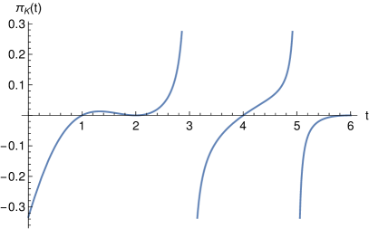
The contribution of $Z_{3}(K)$ to $\beta_{E}$, Eq. (2.3), is found to be

$$\beta_{E}(K\neq 0)=E^{2}\frac{3}{4N_{f}}\int_{0}^{K}\pi_{K}(t)\mathrm{d}t.$$ (3.7)

where we have defined

$$\pi_{K}(t)\equiv\frac{\pi_{K}^{(0)}(t)}{t-3}.$$ (3.8)

We show the function $\pi_{K}(t)$ in Fig. 4. Since $\pi_{K}(t)$ has a first order pole at $t=3$, the first singularity of $\beta_{E}(K\neq 0)$ occurs at $K=3$ and is a logarithmic one. The next singularity of $\pi_{K}(t)$ is found at $t=5$ (first order) and would result in a logarithmic singularity of $\beta_{E}(K\neq 0)$ at $K=5$.

Figure 4: The function $\pi_{K}(t)$ defined in Eq. (3.8).

3.2 The QED contribution to the Yukawa $\beta$-function

The QED contribution to the fermion self-energy and to the Yukawa vertex is closely related to the pure-Yukawa case. This is because the gauge chain is equivalent to the Yukawa chain besides an overall factor. In fact, $\Sigma_{E}^{(n)}$ and $V_{E}^{(n)}$ are related to $\Sigma_{K}^{(n)}$ and $V_{K}^{(n)}$ as

$$\Sigma^{(n)}_{E}(\not{p})= (d-2)\left(\frac{d-2}{d-1}\right)^{n-1}\Sigma_{K}^{(n)}(\not{p}),$$ (3.9)

$$V^{(n)}_{E}(p^{2})= -d\left(\frac{d-2}{d-1}\right)^{n-1}{V_{K}^{(n)}}(p^{2}).$$ (3.10)

The factors $(d-2)$ and $-d$ come from the algebra of the $\gamma$-matrices, while $\left(\frac{d-2}{d-1}\right)^{n-1}$ takes into account the difference in replacing $\Pi_{E}^{(1)}$ with $S_{K}^{(1)}$. Notice that $g_{\mu\nu}$ is the only relevant Lorentz structure in the photon propagator, since the $k_{\mu}k_{\nu}$ term do not contribute to the $\beta$-function.

Making use the relations Eqs (3.9) and (3.10), $\Sigma_{E}^{(n)}$ and $V_{E}^{(n)}$ are expanded as

$$\Sigma^{(n)}_{E}(\not{p})=(-1)^{n-1}\left(\frac{2}{3}\right)^{n}\frac{3}{4n\epsilon^{n}}\sigma_{E}(p^{2},\epsilon,n),$$ (3.11)

$$\sigma_{E}(p^{2},\epsilon,n)=\sum_{j=0}^{\infty}\sigma_{E}^{(j)}(p^{2},\epsilon)(n\epsilon)^{j},$$ (3.12)

and

$$V^{(n)}_{E}(p^{2})=(-1)^{n-1}\frac{3}{n\epsilon^{n}}\left(\frac{2}{3}\right)^{n}v_{E}(p^{2},\epsilon,n),$$ (3.13)

$$v_{E}(p^{2},\epsilon,n)=\sum_{j=0}^{\infty}v_{E}^{(j)}(p^{2},\epsilon)(n\epsilon)^{j}.$$ (3.14)

Using the one-loop result $Z_{E}=\left(1-\frac{2}{3}E\right)^{-1}+\mathcal{O}(1/N_{f})$, and applying the same summation procedure as in Ref. [10] for the fermion self-energy and the vertex, Eqs (2.11) and (2.13) yield

$$Z_{f}(E)=-\frac{1}{N_{f}}\sum_{n=1}^{\infty}\text{div}\left\{(Z_{E}E)^{n}\Sigma_{E}^{(n)}(p^{2},\epsilon)\right\}=-\frac{1}{N_{f}}\frac{3}{4\epsilon}\int_{0}^{\frac{2}{3}E}\sigma_{E}^{(0)}(t)\mathrm{d}t,$$ (3.15)

$$Z_{V}(E)=-\frac{1}{N_{f}}\sum_{n=1}^{\infty}\text{div}\left\{(Z_{E}E)^{n}V_{E}^{(n)}(p^{2},\epsilon)\right\}=-\frac{1}{N_{f}}\frac{3}{\epsilon}\int_{0}^{\frac{2}{3}E}v_{E}^{(0)}(t)\mathrm{d}t,$$ (3.16)

where we kept only the $1/\epsilon$ pole. The functions $\sigma_{E}^{(0)}$ and $v_{E}^{(0)}$ are independent of $p^{2}$, and are given by

$$\sigma_{E}^{(0)}(t)= \frac{2\Gamma(4-t)}{3\pi\Gamma\left(1-\frac{t}{2}\right)\Gamma\left(3-\frac{t}{2}\right)t}\sin\left(\frac{\pi t}{2}\right),$$ (3.17)

$$v_{E}^{(0)}(t)= \left(\frac{1-\frac{t}{4}}{1-\frac{t}{2}}\right)^{2}\sigma_{E}^{(0)}(t).$$ (3.18)

The QED contribution to the scalar self-energy is shown in the second row of Fig. 2. The diagrams involving a horizontal gauge chain are related to the ones in the pure-Yukawa case analogoursly to Eq. (3.9). Altogether, we find

$$S_{E}^{(n)}(p^{2},\epsilon)=(-1)^{n}\left(\frac{2}{3}\right)^{n}\frac{27}{4n(n-1)\epsilon^{n}}s_{E}(p^{2},\epsilon,n),$$ (3.19)

$$s_{E}(p^{2},\epsilon,n)=\sum_{j=0}^{\infty}s_{E}^{(j)}(p^{2},\epsilon)(n\epsilon)^{j}.$$ (3.20)

The QED contribution in Eq. (2.9) is singled out as follows:

$$Z_{S}(E)=-K\text{div}\left\{Z_{f}(E)^{-2}Z_{V}(E)^{2}S_{K}^{(1)}(p^{2},\epsilon)+\frac{1}{N_{f}}\sum_{n=1}^{\infty}(Z_{E}E)^{n}S_{E}^{(n+1)}(p^{2},\epsilon)\right\}.$$ (3.21)

To evaluate the right-hand side of Eq. (3.21), we closely follow the procedure in Ref. [10] for the scalar self-energy:

$$Z_{S}(E) =-\frac{K}{N_{f}}\sum_{n=1}^{\infty}E^{n}\text{div}\left\{\left(1-\frac{2}{3}\frac{E}{\epsilon}\right)^{-n}\left[2S^{(1)}_{F}\left(\Sigma^{(n)}_{E}-V^{(n)}_{E}\right)+S_{E}^{(n+1)}\right]\right\}$$

$$\begin{split}&=-\frac{K}{N_{f}}\sum_{n=1}^{\infty}E^{n}\text{div}\left\{\sum_{i=0}^{n-1}\left(\begin{array}[]{c}n-1\\ i\end{array}\right)\left(\frac{2}{3}\right)^{i}\frac{1}{\epsilon^{i}}\right.\\ &\left.\hskip 93.89418pt\times\left[2S^{(1)}_{F}\left(\Sigma^{(n-i)}_{E}-V^{(n-i)}_{E}\right)+S_{E}^{(n-i+1)}\right]\vphantom{\sum_{i}^{n}}\right\}\end{split}$$ (3.22)

$$=-3\frac{K}{N_{f}}\sum_{n=1}^{\infty}\left(-\frac{2}{3}E\right)^{n}\text{div}\left\{\frac{1}{\epsilon^{n}}\sum_{i=0}^{n-1}\left(\begin{array}[]{c}n-1\\ i\end{array}\right)(-1)^{i}\frac{\xi_{E}(p^{2},\epsilon,n-i)}{(n-i)(n-i+1)\epsilon^{n+1}}\right\},$$ (3.25)

where we defined

$$\xi_{E}(p^{2},\epsilon,n)=\epsilon(n+1)\,2\,S_{F}^{(1)}\left(v_{E}(p^{2},\epsilon,n)-\frac{1}{4}\sigma_{E}(p^{2},\epsilon,n)\right)-\frac{3}{2}s_{E}(p^{2},\epsilon,n+1),$$ (3.26)

and $S_{F}^{(1)}$ is the finite part of the one-loop bubble $S_{K}^{(1)}$.

Figure 5: The functions $\tilde{\xi}_{E}(t)$ (left panel) and $\xi_{E}(t)$ (right panel) defined in Eqs (3.34) and (3.31), respectively.

Then, by expanding

$$\xi_{E}(p^{2},\epsilon,n-i)=\sum_{j=0}^{\infty}\epsilon^{j}(n-i+1)^{j}\xi_{E}^{(j)}(p^{2},\epsilon),$$ (3.27)

and using

$$\sum_{i=0}^{n-1}\left(\begin{array}[]{c}n-1\\ i\end{array}\right)(-1)^{i}\frac{(n-i+1)^{j-1}}{n-i}=\begin{cases}\frac{(-1)^{n+1}}{n+1}&j=0\\ \frac{(-1)^{n+1}}{n}&j=1,..,n\end{cases},$$ (3.28)

we can further simplify the expression to

$$\begin{split}Z_{S}(E)=&3\frac{K}{N_{f}}\sum_{n=1}^{\infty}\left(\frac{2}{3}E\right)^{n}\text{div}\left\{\frac{1}{(n+1)\epsilon^{n+1}}\xi^{(0)}_{E}(p^{2},\epsilon)+\frac{1}{n\epsilon^{n+1}}\sum_{j=1}^{\infty}\xi_{E}^{(j)}(p^{2},\epsilon)\epsilon^{j}\right\}\\ =&\frac{9K}{2EN_{f}}\sum_{n=2}^{\infty}\left(\frac{2}{3}E\right)^{n}\text{div}\left\{\frac{1}{\epsilon^{n}}\left(\frac{\xi_{E}^{(0)}(p^{2},\epsilon)}{n}+\frac{\xi_{E}(p^{2},\epsilon,0)-\xi^{(0)}_{E}(p^{2},\epsilon)}{n-1}\right)\right\}\\ =&\frac{9K}{2EN_{f}}\frac{1}{\epsilon}\int_{0}^{\frac{2}{3}E}\left(\xi_{E}^{(0)}(t)-\xi_{E}^{(0)}(0)+\frac{2}{3}\frac{\xi_{E}(p^{2},t,0)-\xi_{E}^{(0)}(t)}{t}E\right)\mathrm{d}t,\end{split}$$ (3.29)

where we kept the $1/\epsilon$ pole only. The function $\xi_{E}(p^{2},t,0)=\lim_{n\to 0}\xi_{E}(p^{2},t,n)$ has to be independent of $p^{2}$ for the consistency of the computation. This is indeed the case: we checked that

$$\frac{3}{2}s_{E}(p^{2},t,1)=2\left(1+t\,S^{(1)}_{F}(p^{2},t)\right)\left(v_{E}^{(0)}(t)-\frac{1}{4}\sigma_{E}^{(0)}(t)\right),$$ (3.30)

and therefore

$$\xi_{E}(p^{2},t,0)=-2v_{E}^{(0)}(t)+\frac{1}{2}\sigma_{E}^{(0)}(t)\equiv\xi_{E}(t).$$ (3.31)

Finally, we find:

$$Z_{S}(E)=\frac{3K}{\epsilon\,N_{f}}\left\{\frac{3}{2E}\int_{0}^{\frac{2}{3}E}\left(\xi_{E}^{(0)}(t)-\xi_{E}^{(0)}(0)\right)\mathrm{d}t+\int_{0}^{\frac{2}{3}E}\frac{\xi_{E}(t)-\xi_{E}^{(0)}(t)}{t}\mathrm{d}t\right\}.$$ (3.32)

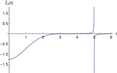
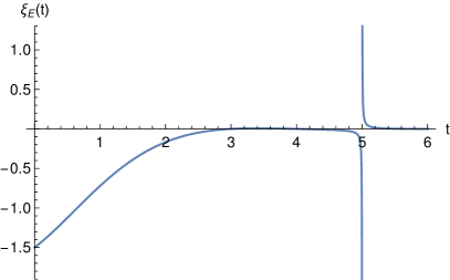
With Eqs (3.15), (3.16) and (3.32) at hand, we can compute the QED contribution to the Yukawa $\beta$-function:

$$\beta_{K}(E\neq 0)=-\frac{3K^{2}}{N_{f}}\left\{\int_{0}^{\frac{2}{3}E}\tilde{\xi}_{E}(t)\mathrm{d}t+\frac{3}{2}+\left(1-\frac{2E}{3K}\right)\xi_{E}\left(\frac{2}{3}E\right)\right\}.$$ (3.33)

where we have defined

$$\tilde{\xi}_{E}(t)\equiv\frac{\xi_{E}(t)-\xi_{E}^{(0)}(t)}{t}.$$ (3.34)

The functions $\xi_{E}(t)$ and $\tilde{\xi}_{E}(t)$ are explicitly given by

$$\xi_{E}(t) =-\frac{2(t-3)^{2}\Gamma(2-t)}{3\Gamma\left(2-\frac{t}{2}\right)\Gamma\left(3-\frac{t}{2}\right)\pi t}\,\sin\left(\frac{\pi t}{2}\right),$$ (3.35)

$$\tilde{\xi}_{E}(t) =\frac{(15+t-5t^{2}+t^{3})\Gamma(4-t)}{9(t-2)\Gamma\left(2-\frac{t}{2}\right)\Gamma(3-\frac{t}{2})\pi t}\sin\left(\frac{\pi t}{2}\right).$$ (3.36)

We plot the functions $\tilde{\xi}_{E}(t)$ and $\xi_{E}(t)$ in Fig. 5. The first singularity of $\beta_{K}(E\neq 0)$ is at $E=15/2$ and consists of a first-order pole coming from $\xi_{E}(t)$ plus a logarithmic singularity arising from the integration of $\tilde{\xi}_{E}(t)$, both at $t=5$.

4 The coupled system

Here we summarize and discuss our results for the coupled system. Combining Eqs (2.15) and (2.16) with the new results in Eqs (3.7) and (3.33), we obtain

$$\frac{\beta_{K}}{K^{2}}= 1-\frac{3}{N_{f}}\left\{1-\frac{1}{3}\int_{0}^{K}\xi_{K}(t)\mathrm{d}t+\int_{0}^{\frac{2}{3}E}\tilde{\xi}_{E}(t)\mathrm{d}t+\left(1-\frac{2E}{3K}\right)\xi_{E}\left(\frac{2}{3}E\right)\right\},$$ (4.1)

$$\frac{\beta_{E}}{E^{2}}= \frac{2}{3}+\frac{1}{4N_{f}}\left\{\int_{0}^{\frac{2}{3}E}\pi_{E}(t)\mathrm{d}t+3\int_{0}^{K}\pi_{K}(t)\mathrm{d}t\right\}.$$ (4.2)

Near the Gaussian fixed point, these can be expanded as

$$\begin{split}\beta_{E}=&\frac{2}{3}E^{2}+\frac{1}{2N_{f}}E^{3}-\frac{1}{4N_{f}}E^{2}K-\frac{11}{72N_{f}}E^{4}+\frac{7}{32N_{f}}E^{2}K^{2}\\ &-\frac{77}{1944N_{f}}E^{5}-\frac{3}{64N_{f}}E^{2}K^{3}+\dots\end{split}$$ (4.3)

$$\begin{split}\beta_{K}=&\left(1+\frac{3}{2N_{f}}\right)K^{2}-\frac{3}{N_{f}}EK-\frac{3}{2N_{f}}K^{3}+\frac{5}{4N_{f}}EK^{2}+\frac{5}{6N_{f}}E^{2}K\\ &+\frac{7}{16N_{f}}K^{4}-\frac{1}{2N_{f}}E^{2}K^{2}+\frac{35}{108N_{f}}E^{3}K\\ &+\frac{11}{96N_{f}}K^{5}+\frac{1}{3888N_{f}}\left(-1625+1296\zeta_{3}\right)E^{3}K^{2}+\frac{1}{648N_{f}}(83-144\zeta_{3})E^{4}K\dots\end{split}$$ (4.4)

We have checked that the expansions agree with the known four-loop results [19, 20, 21, 22, 23] in the leading order in $N_{f}$. Furthermore, the $-\frac{2E}{3K}\xi_{E}\left(\frac{2}{3}E\right)$ part in the last term of Eq. (4.1) corresponds to the result of Refs [11, 12], and we have checked that our result agrees with those.

The first singularity of the pure-QED $\beta$-function is located at $E=15/2$, whereas for the pure-Yukawa case it occurs at $K=5$. These known singularities are now accompanied by the ones from the mixed contributions, Eqs (3.7) and (3.33). As we noticed in Section 3, $\beta_{E}(K\neq 0)$ has the first singularity at $K=3$, while $\beta_{K}(E\neq 0)$ at $E=15/2$. The former, similarly to the pure gauge and Yukawa cases, is a logarithmic singularity, whereas the latter is a pole of first order.

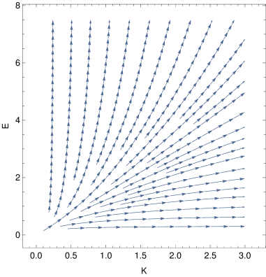
The $\mathcal{O}(1/N_{f})$ coupled system has only the three already known fixed points: the Gaussian fixed point, and the pure-QED (near $E=15/2$) and pure-Yukawa (near $K=3$) fixed points.

We show the flow diagram for $N_{f}=30$ outside the vicinity of the singularities in Fig. 6. Near $K=3$, the logarithmic singularity in $\beta_{E}$ arising from $\pi_{K}(t)$ dominates making the gauge coupling to increase and approach the value $E=15/2$. Near $E=15/2$, however, $\beta_{K}$ has a pole arising from $\xi_{E}(t)$ eventually dominating the flow, and driving the Yukawa coupling to zero near $E=15/2$. The flow may be extended setting $K\equiv 0$ and switching to pure-QED, so that the gauge coupling reaches the fixed point as $E\to 15/2$ in the UV.

Figure 6: The flow diagram for the coupled system with $N_{f}=30$. The arrows point towards UV.

5 Conclusions

We have computed the leading $1/N_{f}$ mixed contributions for the $\beta$-functions for abelian gauge-Yukawa theory with $N_{f}$ fermion flavours coupling to a gauge-singlet real scalar. Together with the known results for the pure-QED and pure-Yukawa cases, this allows the study of the abelian gauge-Yukawa system.

The flow in the interacting theory leads to the vanishing Yukawa coupling near the gauge coupling value $E=15/2$ due to the peculiar interplay of the singularities. However, the gauge $\beta$-function is still positive around $(K,E)=(0,15/2)$, and $E$ keeps growing before eventually reaching the fixed point due to the known a logarithmic singluarity near $E=15/2$.

Our work extends the previous results towards a more complete picture of gauge-Yukawa theories in the large-$N_{f}$ limit.

References

- [1] D. F. Litim and F. Sannino, Asymptotic safety guaranteed, JHEP 12 (2014) 178, [arXiv:1406.2337].
- [2] R. Mann, J. Meffe, F. Sannino, T. Steele, Z.-W. Wang, and C. Zhang, Asymptotically Safe Standard Model via Vectorlike Fermions, Phys. Rev. Lett. 119 (2017), no. 26 261802, [arXiv:1707.02942].
- [3] G. M. Pelaggi, A. D. Plascencia, A. Salvio, F. Sannino, J. Smirnov, and A. Strumia, Asymptotically Safe Standard Model Extensions?, Phys. Rev. D97 (2018), no. 9 095013, [arXiv:1708.00437].
- [4] O. Antipin and F. Sannino, Conformal Window 2.0: The large safe story, Phys. Rev. D97 (2018), no. 11 116007, [arXiv:1709.02354].
- [5] D. Espriu, A. Palanques-Mestre, P. Pascual, and R. Tarrach, The Function in the 1/ Expansion, Z. Phys. C13 (1982) 153.
- [6] A. Palanques-Mestre and P. Pascual, The 1/ Expansion of the and Beta Functions in QED, Commun. Math. Phys. 95 (1984) 277.
- [7] J. A. Gracey, The QCD -function at O(1/), Phys. Lett. B373 (1996) 178–184, [hep-ph/9602214].
- [8] B. Holdom, Large N flavor beta-functions: a recap, Phys. Lett. B694 (2011) 74–79, [arXiv:1006.2119].
- [9] R. Shrock, Study of Possible Ultraviolet Zero of the Beta Function in Gauge Theories with Many Fermions, Phys. Rev. D89 (2014), no. 4 045019, [arXiv:1311.5268].
- [10] T. Alanne and S. Blasi, The -function for Yukawa theory at large , arXiv:1806.06954.
- [11] K. Kowalska and E. M. Sessolo, Gauge contribution to the 1/NF expansion of the Yukawa coupling beta function, JHEP 04 (2018) 027, [arXiv:1712.06859].
- [12] O. Antipin, N. A. Dondi, F. Sannino, A. E. Thomsen, and Z.-W. Wang, Gauge-Yukawa theories: Beta functions at large , Phys. Rev. D98 (2018), no. 1 016003, [arXiv:1803.09770].
- [13] J. A. Gracey, Calculation of exponent eta to O(1/N**2) in the O(N) Gross-Neveu model, Int. J. Mod. Phys. A6 (1991) 395–408. [Erratum: Int. J. Mod. Phys.A6,2755(1991)].
- [14] A. N. Vasiliev, S. E. Derkachov, N. A. Kivel, and A. S. Stepanenko, The 1/n expansion in the Gross-Neveu model: Conformal bootstrap calculation of the index eta in order 1/n**3, Theor. Math. Phys. 94 (1993) 127–136. [Teor. Mat. Fiz.94,179(1993)].
- [15] J. A. Gracey, Computation of Beta-prime (g(c)) at O(1/N**2) in the O(N) Gross-Neveu model in arbitrary dimensions, Int. J. Mod. Phys. A9 (1994) 567–590, [hep-th/9306106].
- [16] J. A. Gracey, Computation of critical exponent eta at O(1/N**3) in the four Fermi model in arbitrary dimensions, Int. J. Mod. Phys. A9 (1994) 727–744, [hep-th/9306107].
- [17] J. A. Gracey, Critical exponent in the Gross-Neveu-Yukawa model at , Phys. Rev. D96 (2017), no. 6 065015, [arXiv:1707.05275].
- [18] A. N. Manashov and M. Strohmaier, Correction exponents in the Gross–Neveu–Yukawa model at , Eur. Phys. J. C78 (2018), no. 6 454, [arXiv:1711.02493].
- [19] M. E. Machacek and M. T. Vaughn, Two Loop Renormalization Group Equations in a General Quantum Field Theory. 1. Wave Function Renormalization, Nucl. Phys. B222 (1983) 83–103.
- [20] M. E. Machacek and M. T. Vaughn, Two Loop Renormalization Group Equations in a General Quantum Field Theory. 2. Yukawa Couplings, Nucl. Phys. B236 (1984) 221–232.
- [21] A. G. M. Pickering, J. A. Gracey, and D. R. T. Jones, Three loop gauge beta function for the most general single gauge coupling theory, Phys. Lett. B510 (2001) 347–354, [hep-ph/0104247]. [Erratum: Phys. Lett.B535,377(2002)].
- [22] K. G. Chetyrkin and M. F. Zoller, Three-loop -functions for top-Yukawa and the Higgs self-interaction in the Standard Model, JHEP 06 (2012) 033, [arXiv:1205.2892].
- [23] N. Zerf, P. Marquard, R. Boyack, and J. Maciejko, Critical behavior of the QED3-Gross-Neveu-Yukawa model at four loops, arXiv:1808.00549.