Physical-density integral equation methods for scattering from multi-dielectric cylinders

Abstract

An integral equation-based numerical method for scattering from multi-dielectric cylinders is presented. Electromagnetic fields are represented via layer potentials in terms of surface densities with physical interpretations. The existence of null-field representations then adds superior flexibility to the modeling. Local representations are used for fast field evaluation at points away from their sources. Partially global representations, constructed as to reduce the strength of kernel singularities, are used for near-evaluations. A mix of local- and partially global representations is also used to derive the system of integral equations from which the physical densities are solved. Unique solvability is proven for the special case of scattering from a homogeneous cylinder under rather general conditions. High achievable accuracy is demonstrated for several examples found in the literature.

1 Introduction

Integral equation methods based on local and global integral representations of electromagnetic fields are presented for the two-dimensional transmission setting of an incident time harmonic transverse magnetic wave that is scattered from an object consisting of an arbitrary number of homogeneous dielectric regions. Several numerical difficulties are encountered in the evaluations of the electric and magnetic fields outside and inside the object. That places high demands on the choice of integral equations, integral representations, and numerical techniques.

It was seen in [7], where scattering from a homogeneous object was treated, that uniqueness- and numerical problems may occur for objects having complex permittivities. In that paper the key to these problems was a system of integral equations for surface densities without physical interpretation (an indirect formulation with abstract densities). We now show that uniqueness statements and accurate field evaluations can also be obtained using a system of integral equations for surface densities with physical interpretation (a direct formulation with physical densities). This is an important step since direct formulations can deliver even higher field accuracy than can indirect formulations.

Other important results of this paper concern objects that consist of more than one dielectric region. Three major numerical challenges are encountered. The first is to accurately evaluate the electric and magnetic fields close to boundaries. The second is to find and solve integral equations for objects with boundary triple junctions, and to evaluate fields close to such points. The third is to accurately evaluate the electric field when contrasts between regions are very high. The integral representations and equations we have developed to meet these challenges are based upon physical surface densities and global layer potentials. The advantage with our global layer potentials is that they can be combined to have weaker singularities in their kernels in more situations than can other layer potentials.

The numerical challenges that remain after our careful modeling are taken care of by Nyström discretization, accelerated with recursively compressed inverse preconditioning, and product integration. Numerical examples constitute an important part of the paper since they verify that our choices of integral representations and equations are indeed efficient and can handle all of the difficulties described above.

The present work can be viewed as a continuation of the work [7], on scattering from homogeneous objects, which uses several results from [12] and [15]. Two new integral equation formulations have recently been applied to problems that are similar to the present scattering problem. The first is referred to as the multi-trace formulation (MTF). It is based upon a system of Fredholm first-kind equations, that by a Calderón diagonal preconditioner can be transformed into a system of second-kind equations [2, 10]. The other is the single-trace formulation (STF). It is based on a system of Fredholm second-kind equations for abstract layer potentials [10]. An approach similar to the STF is presented in [5]. Special attention is given to numerical problems that arise at triple junctions, and in that respect Refs. [2, 5, 10] have much in common with the present work. A difference is that our representations lead to cancellation of kernel singularities at field points close to boundaries, which is important for accurate field evaluations.

The paper is organized as follows: Section 2 details the problem to be solved. Physical surface densities and regional and global layer potentials and integral operators are reviewed in Section 3. Section 4 introduces local integral representations and null-fields. These are assembled and used for the construction of integral equations with global integral operators in Section 5, which also contains the proof of unique solvability for the special case of a homogeneous object. Sections 6 and 7 are on the evaluation of electromagnetic fields. Section 8 shows that certain contributions to global integral representations and operators are superfluous and can be removed for better numerical performance. Section 9 reviews discretization techniques. Section 10 puts our integral equations into a broader context by comparing them with popular formulations for the Maxwell transmission problem in three dimensions. Our methods are then tested in three well-documented numerical examples in Section 11. Section 12 contains conclusions.

2 Problem formulation

This section presents the problem we shall solve as a partial differential equation (PDE) and reviews relations between magnetic and electric fields.

2.1 Geometry and unit vectors

The geometry is in $\mathbb{R}^{2}$ and consists of a bounded object composed of $N-1$ dielectric regions $\Omega_{n}$, $n=2,\ldots,N$, which is surrounded by an unbounded dielectric region $\Omega_{1}$. A point in $\mathbb{R}^{2}$ is denoted $r=(x,y)$. Each region $\Omega_{n}$ has unit relative permeability and is characterized by its relative permittivity $\varepsilon(r)=\varepsilon_{n}$, $r\in\Omega_{n}$, $n=1,\ldots,N$.

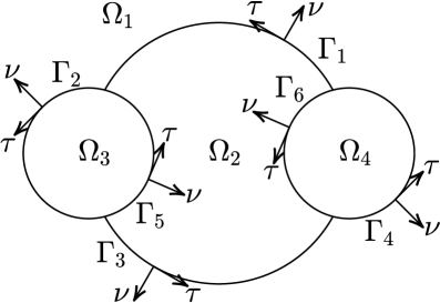
Figure 1: The boundaries $\Gamma$ of a four-region configuration with tangential and normal unit vectors $\tau$ and $\nu$. The closed curves ${\cal C}_{n}$ consist of subcurves $\Gamma_{m}$: ${\cal C}_{1}=\Gamma_{1}\cup\Gamma_{2}\cup\Gamma_{3}\cup\Gamma_{4}$, ${\cal C}_{2}=\Gamma_{1}\cup\Gamma_{5}\cup\Gamma_{3}\cup\Gamma_{6}$, ${\cal C}_{3}=\Gamma_{2}\cup\Gamma_{5}$, and ${\cal C}_{4}=\Gamma_{4}\cup\Gamma_{6}$.

The regions $\Omega_{n}$, $n\geq 2$, are bounded by closed curves ${\cal C}_{n}$ that consist of subcurves $\Gamma_{m}$, see Figure 1 for an example. The total number of subcurves is $M$ and their union is denoted $\Gamma$. The closed curve ${\cal C}_{1}$, bounding the region $\Omega_{1}$, is the outer boundary of the object (the point at infinity is not included). If a closed curve ${\cal C}_{n}$ is traversed so that $\Omega_{n}$ is on the right, we say that ${\cal C}_{n}$ is traversed in a clockwise direction. The opposite direction is called counterclockwise. Note that this definition of clockwise and counterclockwise agrees with intuition for all ${\cal C}_{n}$, seen as isolated closed curves, except for ${\cal C}_{1}$.

Each subcurve $\Gamma_{m}$ has a tangential unit vector $\tau=(\tau_{x},\tau_{y})$ that defines the orientation of $\Gamma_{m}$ and a normal unit vector $\nu=(\nu_{x},\nu_{y})$ that points to the right with respect to the orientation of $\Gamma_{m}$, as in Figure 1. We shall also use the standard basis in $\mathbb{R}^{3}$ with $\hat{{\boldsymbol{x}}}=(1,0,0)$, $\hat{{\boldsymbol{y}}}=(0,1,0)$, and $\hat{{\boldsymbol{z}}}=(0,0,1)$. The vectors $\tau$ and $\nu$ are related by

$${\boldsymbol{\tau}}=\hat{{\boldsymbol{z}}}\times{\boldsymbol{\nu}},$$ (1)

where ${\boldsymbol{\tau}}=(\tau_{x},\tau_{y},0)$ and ${\boldsymbol{\nu}}=(\nu_{x},\nu_{y},0)$.

2.2 PDE formulation of the transmission problem

The aim is to find the magnetic and electric fields, ${\boldsymbol{H}}(r)$ and ${\boldsymbol{E}}(r)$, in all regions $\Omega_{n}$, given an incident time-harmonic transverse magnetic (TM) plane wave. Both ${\boldsymbol{E}}$ and ${\boldsymbol{H}}$ can be expressed in terms of a scalar field $U(r)$. The vacuum wavenumber is denoted $k_{0}$ and the wavenumbers in the regions are

$$k(r)=k_{n}\equiv\sqrt{\varepsilon_{n}}k_{0}\,,\quad r\in\Omega_{n}\,,\quad n=1,\ldots,N\,.$$ (2)

For $r\in\Gamma_{m}$ we define $U^{\rm R}(r)$, $\nabla U^{\rm R}(r)$, $k_{m}^{\rm R}$, and $\varepsilon_{m}^{R}$ as the limit scalar field, the limit gradient field, the wavenumber, and the permittivity on the right-hand side of $\Gamma_{m}$. On the left-hand side of $\Gamma_{m}$ the corresponding quantities are $U^{\rm L}(r)$, $\nabla U^{\rm L}(r)$, $k_{m}^{\rm L}$, and $\varepsilon_{m}^{L}$.

The PDE for the scalar field is

$$\Delta U(r)+k(r)^{2}U(r) =0\,,\quad r\in\mathbb{R}^{2}\setminus\Gamma\,,$$ (3)

with boundary conditions on $\Gamma_{m}$, $m=1,\ldots,M$,

$$U^{\rm R}(r) =U^{\rm L}(r)\,,\quad r\in\Gamma_{m}\,,$$ (4)

$$(\varepsilon_{m}^{\rm R})^{-1}\nu\cdot\nabla U^{\rm R}(r) =(\varepsilon_{m}^{\rm L})^{-1}\nu\cdot\nabla U^{\rm L}(r)\,,\quad r\in\Gamma_{m}\,.$$ (5)

In $\Omega_{1}$ the field is decomposed into an incident and a scattered field

$$U(r)=U^{\rm in}(r)+U^{\rm sc}(r)\,,\quad r\in\Omega_{1},$$ (6)

where

$$\Delta U^{\rm in}(r)+k_{1}^{2}U^{\rm in}(r) =0\,,\quad r\in\mathbb{R}^{2}\,.$$ (7)

The scattered field satisfies the radiation condition

$$\lim_{|r|\to\infty}\sqrt{|r|}\left(\frac{\partial}{\partial|r|}-{\rm i}k_{1}\right)U^{\rm sc}(r)=0\,,\quad r\in\Omega_{1}\,.$$ (8)

The time dependence $e^{-{\rm i}t}$ is assumed and the angular frequency is scaled to one.

2.3 The magnetic and electric fields

The complex magnetic and electric fields are

$${\boldsymbol{H}}(r) =U(r)\hat{{\boldsymbol{z}}}\,,\quad r\in\mathbb{R}^{2}\,,$$ (9)

$${\boldsymbol{E}}(r) ={\rm i}k_{0}^{-1}\varepsilon_{n}^{-1}\nabla_{3}U(r)\times\hat{{\boldsymbol{z}}}\,,\quad r\in\Omega_{n}\,,$$ (10)

where the $\nabla_{3}U(r)$ is the gradient $\nabla U(r)$ extended with a zero third component. The corresponding time-domain fields are

$${\boldsymbol{H}}(r,t) =\Re{\rm e}\{{\boldsymbol{H}}(r)e^{-{\rm i}t}\}\,,$$ (11)

$${\boldsymbol{E}}(r,t) =\Re{\rm e}\{{\boldsymbol{E}}(r)e^{-{\rm i}t}\}\,.$$ (12)

The electric field is scaled with the wave impedance of vacuum, $\eta_{0}$, in order to give the magnetic and electric fields the same dimension.

2.4 The incident plane wave

The incident TM-wave travels in the direction $d=(d_{x},d_{y})$, and the scalar field $U^{\rm in}$, magnetic field ${\boldsymbol{H}}^{\rm in}$, and electric field ${\boldsymbol{E}}^{\rm in}$ of this wave are

$$U^{\rm in}(r)=e^{{\rm i}k_{1}(d\cdot r)}\,,$$ (13)

$${\boldsymbol{H}}^{\rm in}(r)=e^{{\rm i}k_{1}(d\cdot r)}\hat{{\boldsymbol{z}}}\,,$$ (14)

$${\boldsymbol{E}}^{\rm in}(r)=\dfrac{1}{\sqrt{\varepsilon_{1}}}(-d_{y},d_{x},0)e^{{\rm i}k_{1}(d\cdot r)}\,.$$ (15)

The normal component of the incident electric field on a boundary is

$${\boldsymbol{\nu}}\cdot{\boldsymbol{E}}^{\rm in}(r)=\dfrac{1}{\sqrt{\varepsilon_{1}}}(\nu_{y}d_{x}-\nu_{x}d_{y})e^{{\rm i}k_{1}(d\cdot r)}\,.$$ (16)

3 Physical densities, potentials, and operators

Two surface densities, $\mu(r)$ and $\rho(r)$, are introduced and referred to as physical densities. The density $\mu$ is the tangential component of ${\boldsymbol{H}}$ and the density $\rho$ is proportional to the tangential component of ${\boldsymbol{E}}$

$$\mu(r)=U(r)\,,\quad r\in\Gamma_{m}\,,$$ (17)

$$\rho(r)=(\varepsilon_{m}^{\rm R})^{-1}\nu\cdot\nabla U^{\rm R}(r)\,,\quad r\in\Gamma_{m}\,.$$ (18)

If $U$ is a solution to the transmission problem of Section 2.2 it also holds, because of (5), that

$$\rho(r)=(\varepsilon_{m}^{\rm L})^{-1}\nu\cdot\nabla U^{\rm L}(r)\,,\quad r\in\Gamma_{m}\,.$$ (19)

In [7] it was shown that integral equation-based numerical schemes involving physical densities offer certain advantages for field evaluations close to $\Gamma$, compared to indirect schemes involving surface densities without immediate physical interpretations (abstract densities). We here pursue the concept of physical densities.

3.1 Acoustic layer potentials and operators

The fundamental solution to the Helmholtz equation is taken as

$$\Phi_{k}(r,r^{\prime})=\frac{\rm i}{2}H_{0}^{(1)}(k|r-r^{\prime}|)\,,$$ (20)

where $H_{0}^{(1)}$ is the zeroth order Hankel function of the first kind. On each subcurve $\Gamma_{m}$ we need six right-hand acoustic layer potentials defined in terms of a general surface density $\sigma(r)$ as

$$S_{m}^{\rm R}\sigma(r) =\int_{\Gamma_{m}}\Phi_{k_{m}^{\rm R}}(r,r^{\prime})\sigma(r^{\prime})\,{\rm d}\ell^{\prime}\,,$$ (21)

$$K_{m}^{\rm R}\sigma(r) =\int_{\Gamma_{m}}\frac{\partial\Phi_{k_{m}^{\rm R}}}{\partial\nu^{\prime}}(r,r^{\prime})\sigma(r^{\prime})\,{\rm d}\ell^{\prime}\,,$$ (22)

$$K^{\rm RA}_{m}\sigma(r) =\int_{\Gamma_{m}}\frac{\partial\Phi_{k_{m}^{\rm R}}}{\partial\nu}(r,r^{\prime})\sigma(r^{\prime})\,{\rm d}\ell^{\prime}\,,$$ (23)

$$T_{m}^{\rm R}\sigma(r) =\int_{\Gamma_{m}}\frac{\partial^{2}\Phi_{k_{m}^{\rm R}}}{\partial\nu\partial\nu^{\prime}}(r,r^{\prime})\sigma(r^{\prime})\,{\rm d}\ell^{\prime},$$ (24)

$${\boldsymbol{B}}_{m}^{\rm R}\sigma(r) =\int_{\Gamma_{m}}\Phi_{k_{m}^{\rm R}}(r,r^{\prime}){\boldsymbol{\tau}}(r^{\prime})\sigma(r^{\prime})\,{\rm d}\ell^{\prime}\,,$$ (25)

$$C_{m}^{\rm R}\sigma(r) =\int_{\Gamma_{m}}\frac{\partial\Phi_{k_{m}^{\rm R}}}{\partial\tau}(r,r^{\prime})\sigma(r^{\prime})\,{\rm d}\ell^{\prime}\,.$$ (26)

Here $r\in\mathbb{R}^{2}$, $\partial/\partial\nu^{\prime}=\nu(r^{\prime})\cdot\nabla^{\prime}$, $\partial/\partial\nu=\nu(r)\cdot\nabla$, $\partial/\partial\tau=\tau(r)\cdot\nabla$, and we have extended the definition of the rightward unit normal $\nu=\nu(r)$ at a point $r\in\Gamma$ so that if $r\notin\Gamma$, then $\nu$ is to be interpreted as an arbitrary unit vector associated with $r$. The left-hand layer potentials $S_{m}^{\rm L}\sigma(r)$, $K_{m}^{\rm L}\sigma(r)$, $K_{m}^{\rm LA}\sigma(r)$, $T_{m}^{\rm L}\sigma(r)$, ${\boldsymbol{B}}_{m}^{\rm L}\sigma(r)$, and $C_{m}^{\rm L}\sigma(r)$ are defined analogously to the right-hand potentials.

For each closed curve ${\cal C}_{n}$ we now define the six regional layer potentials $S_{n}\sigma(r)$, $K_{n}\sigma(r)$, $K^{\rm A}_{n}\sigma(r)$, $T_{n}\sigma(r)$, ${\boldsymbol{B}}_{n}\sigma(r)$, and $C_{n}\sigma(r)$ via

$$G_{n}\sigma(r)=\sum\limits_{{\rm ccw}\,\Gamma_{m}\in{\cal C}_{n}}G_{m}^{\rm L}\sigma(r)-\sum\limits_{{\rm cw}\,\Gamma_{m}\in{\cal C}_{n}}G_{m}^{\rm R}\sigma(r)\,,\quad r\in\mathbb{R}^{2}\,,$$ (27)

where $G$ can represent $S$, $K$, $K^{\rm A}$, $T$, ${\boldsymbol{B}}$, and $C$ and where “${\rm cw}\,\Gamma_{m}$” and “${\rm ccw}\,\Gamma_{m}$” denote subcurves with clockwise and counterclockwise orientations along ${\cal C}_{n}$. For the special case of $r\in\Gamma$ we refer to the $G_{n}$ of (27) as integral operators.

When $r^{\circ}\in{\cal C}_{n}$, and with some abuse of notation, one can show the limits

$$\begin{split}\lim_{\Omega_{n}\ni r\to r^{\circ}}S_{n}\sigma(r)&=S_{n}\sigma(r^{\circ})\,,\\ \lim_{\Omega_{n}\ni r\to r^{\circ}}K_{n}\sigma(r)&=-\sigma(r^{\circ})+K_{n}\sigma(r^{\circ})\,,\\ \lim_{\Omega_{n}\ni r\to r^{\circ}}K_{n}^{\rm A}\sigma(r)&=\sigma(r^{\circ})+K_{n}^{\rm A}\sigma(r^{\circ})\,,\\ \lim_{\Omega_{n}\ni r\to r^{\circ}}T_{n}\sigma(r)&=T_{n}\sigma(r^{\circ})\,,\\ \lim_{\Omega_{n}\ni r\to r^{\circ}}C_{n}\sigma(r)&=C_{n}\sigma(r^{\circ})\,,\\ \lim_{\Omega_{n}\ni r\to r^{\circ}}{\boldsymbol{B}}_{n}\sigma(r)&={\boldsymbol{B}}_{n}\sigma(r^{\circ})\,.\end{split}$$ (28)

Here $C_{n}\sigma(r^{\circ})$ is to be understood in the Cauchy principal-value sense and $T_{n}\sigma(r^{\circ})$ in the Hadamard finite-part sense. See [4, Theorem 3.1] and [3, Theorem 2.21] for more precise statements on these limits and [11, Theorem 5.46] for statements in a modern function-space setting.

3.2 The singular nature of kernels

In a similar way as in the indirect approach of [5, Section 3] and [10, Section 3.2], we plan to derive a global integral representation of the scalar field $U$. A global representation means that the densities $\mu(r)$ and $\rho(r)$ are used to represent $U$ in every region $\Omega_{n}$, whether $r$ is on the boundary of that region or not [5]. For this, we need to introduce global layer potentials and integral operators, which are sums over their regional counterparts. This section, which draws on [7, Section 4], collects known results on the singular nature of kernels of various potentials and operators that occur in our representations of $U$ and ${\boldsymbol{E}}$ and in our integral equations for $\mu$ and $\rho$.

The kernels of the global layer potentials

$$\sum_{n=1}^{N}\varepsilon_{n}S_{n}\sigma(r)\,,\quad\sum_{n=1}^{N}K_{n}\sigma(r)\,,\quad r\in\mathbb{R}^{2}\setminus\Gamma\,,$$ (29)

exhibit logarithmic singularities as $r\to r^{\prime}\in\Gamma$. This is so since $\Phi_{k}(r,r^{\prime})$ of (20) has a logarithmic singularity as $r\to r^{\prime}$ and this singularity carries over to the kernel of $S_{n}\sigma(r)$. From (27) it follows that

$$\sum_{n=1}^{N}K_{n}\sigma(r)=\sum_{m=1}^{M}\left(K_{m}^{\rm L}-K_{m}^{\rm R}\right)\sigma(r)\,.$$ (30)

In each term in the sum on the right-hand side of (30) the leading Cauchy-singular parts of the kernels of $K_{m}^{\rm L}\sigma(r)$ and $K_{m}^{\rm R}\sigma(r)$ are independent of the wavenumber, see [7, Section 4.3], and cancel out. Changing the order of summation in global layer potentials, as in (30), is helpful when studying their singularities.

The kernel of

$$\sum_{n=1}^{N}\varepsilon_{n}\partial_{i}S_{n}\sigma(r)\,,\quad r\in\mathbb{R}^{2}\setminus\Gamma\,,\quad i=x,y\,,$$ (31)

exhibits logarithmic- and Cauchy-type singularities as $r\to r^{\prime}\in\Gamma$. The kernel of

$$\sum_{n=1}^{N}\partial_{i}K_{n}\sigma(r)\,,\quad r\in\mathbb{R}^{2}\setminus\Gamma\,,\quad i=x,y\,,$$ (32)

exhibits, strictly speaking, only logarithmic singularities as $r\to r^{\prime}\in\Gamma$. In the context of numerical product integration, however, it is advantageous to consider this kernel as having a Cauchy-type singularity. See [7, Section 4.5]. The kernels of $\partial_{i}S_{n}\sigma(r)$, $i=x,y\,$, exhibit logarithmic- and Cauchy-type singularities as $\Omega_{n}\ni r\to r^{\prime}\in{\cal C}_{n}$. The kernel of ${\boldsymbol{B}}_{n}\sigma(r)$ exhibits logarithmic singularities as $\Omega_{n}\ni r\to r^{\prime}\in{\cal C}_{n}$.

The global integral operators

$$\sum_{n=1}^{N}S_{n}\,,\quad\sum_{n=1}^{N}T_{n}\,,\quad\sum_{n=1}^{N}C_{n}\,,\quad\sum_{n=1}^{N}{\boldsymbol{B}}_{n}\,,$$ (33)

have weakly singular (logarithmic) kernels and are compact, while

$$\sum_{n=1}^{N}\varepsilon_{n}^{-1}K_{n}\,,\quad\sum_{n=1}^{N}\varepsilon_{n}K_{n}^{\rm A}\,,\quad\sum_{n=1}^{N}\varepsilon_{n}^{-1}K_{n}^{\rm A}\,,$$ (34)

are merely bounded. Away from singular boundary points, such as corners or triple junctions, these latter operators also have weakly singular (logarithmic) kernels and are compact. See [17, Lemmas 1-2] for similar statements on boundaries of simply connected Lipschitz domains.

4 Integral representations of $U$ and $\nu\cdot\nabla U$

If $U$ is a solution to the transmission problem of Section 2.2, Green’s theorem and (17), (18), and (19), give the local integral representation

$$U(r)=U^{\rm in}(r)\delta_{n1}-\frac{1}{2}\left(K_{n}\mu(r)-\varepsilon_{n}S_{n}\rho(r)\right)\,,\quad r\in\Omega_{n}\,,$$ (35)

see [16, Section 3.1] and [12, Section 4.2]. A local representation means that only the parts of the densities $\mu$ and $\rho$ that are present on ${\cal C}_{n}$ are used to represent $U$ in $\Omega_{n}$. For $r$ outside $\Omega_{n}$ Green’s theorem gives

$$\begin{split}0=&U^{\rm in}(r)\delta_{n1}-\frac{1}{2}\left(K_{n}\mu(r)-\varepsilon_{n}S_{n}\rho(r)\right)\,,\quad r\notin\Omega_{n}\cup{\cal C}_{n}\,.\end{split}$$ (36)

This relation is well-known, but by many different names, such as the extinction theorem, the Ewald-Oseen extinction theorem [1, Chapter 2.4], the Helmholtz formulae [18], the null-field equation [13], and the extended boundary condition [23]. We can add the right-hand side of (36) to the field in regions outside $\Omega_{n}$ without altering the field. This opens up possibilities to weaken singularities in integral equations and near singularities in integral representations. In what follows we often use this opportunity to improve accuracy in the evaluation of magnetic and electric fields.

The directional derivative of (35) and (36) are

$$\nu\cdot\nabla U(r)=\nu\cdot\nabla U^{\rm in}(r)\delta_{n1}-\frac{1}{2}\left(T_{n}\mu(r)-\varepsilon_{n}K_{n}^{\rm A}\rho(r)\right),\quad r\in\Omega_{n}\,,$$ (37)

and

$$0=\nu\cdot\nabla U^{\rm in}(r)\delta_{n1}-\frac{1}{2}\left(T_{n}\mu(r)-\varepsilon_{n}K_{n}^{\rm A}\rho(r)\right),\quad r\notin\Omega_{n}\cup{\cal C}_{n}\,,$$ (38)

where $\nu=\nu(r)$ is an arbitrary unit vector associated with $r$.

In summary we can say that if $U$ is a solution to the transmission problem of Section 2.2, then (35), (36), (37), and (38) hold for $r\in\mathbb{R}^{2}\setminus\Gamma$.

5 Integral equations

When $\Omega_{n}\ni r\to{\cal C}_{n}$ in (35) and (37), each boundary ${\cal C}_{n}$ gives rise to two separate integral equations

$$\mu(r)+K_{n}\mu(r)-\varepsilon_{n}S_{n}\rho(r)=2U^{\rm in}(r)\delta_{n1}\,,\quad r\in{\cal C}_{n}\,,$$ (39)

$$\varepsilon_{n}\rho(r)+T_{n}\mu(r)-\varepsilon_{n}K_{n}^{\rm A}\rho(r)=2\nu\cdot\nabla U^{\rm in}(r)\delta_{n1}\,,\quad r\in{\cal C}_{n}\,.$$ (40)

The $2N$ equations (39) and (40) and the null-field representations (36) and (38) are now combined into a single system of integral equations. We first show how this is done for $N=2$, that is for a homogeneous object, and then proceed to objects with many regions.

5.1 Integral equations and uniqueness when $N=2$

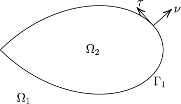
Figure 2: The boundary $\Gamma=\Gamma_{1}={\cal C}_{1}={\cal C}_{2}$ of a two-region configuration with tangential and normal unit vectors $\tau$ and $\nu$.

When $N=2$, then $\Omega_{1}$ is the outer region, $\Omega_{2}$ is the object, and there is only one boundary $\Gamma=\Gamma_{1}={\cal C}_{1}={\cal C}_{2}$. See Figure 2 for an example. First we add $\varepsilon_{1}^{-1}$ times (39) for ${\cal C}_{1}$ and $c\varepsilon_{2}^{-1}$ times (39) for ${\cal C}_{2}$. Here $c$ is a free parameter such that $c\varepsilon_{1}+\varepsilon_{2}\neq 0$. This gives

$$\mu(r)+\breve{\alpha}_{1}\left(\varepsilon_{1}^{-1}K_{1}+c\varepsilon_{2}^{-1}K_{2}\right)\mu(r)-\breve{\alpha}_{1}\left(S_{1}+cS_{2}\right)\rho(r)=f_{1}(r)\,,\quad r\in\Gamma\,,$$ (41)

where

$$\breve{\alpha}_{1}=\frac{\varepsilon_{1}\varepsilon_{2}}{c\varepsilon_{1}+\varepsilon_{2}}\,,\quad f_{1}(r)=2\breve{\alpha}_{1}\varepsilon_{1}^{-1}U^{\rm in}(r)\,.$$ (42)

The other integral equation is the sum of the ${\cal C}_{1}$ and ${\cal C}_{2}$ versions of (40)

$$\rho(r)+\beta_{1}(T_{1}+T_{2})\mu(r)-\beta_{1}\left(\varepsilon_{1}K_{1}^{\rm A}+\varepsilon_{2}K_{2}^{\rm A}\right)\rho(r)=f_{2}(r)\,,\quad r\in\Gamma\,,$$ (43)

where

$$\beta_{1}=\frac{1}{\varepsilon_{1}+\varepsilon_{2}}\,,\quad f_{2}(r)=2\beta_{1}\nu\cdot\nabla U^{\rm in}(r)\,.$$ (44)

We now write the system of integral equations (41) and (43) in block-matrix form

$$\begin{bmatrix}I+\breve{\alpha}_{1}\left(\varepsilon_{1}^{-1}K_{1}+c\varepsilon_{2}^{-1}K_{2}\right)&-\breve{\alpha}_{1}\left(S_{1}+cS_{2}\right)\\ \beta_{1}(T_{1}+T_{2})&I-\beta_{1}\left(\varepsilon_{1}K_{1}^{\rm A}+\varepsilon_{2}K_{2}^{\rm A}\right)\end{bmatrix}\begin{bmatrix}\mu(r)\\ \rho(r)\end{bmatrix}=\begin{bmatrix}f_{1}(r)\\ f_{2}(r)\end{bmatrix},$$ (45)

where the diagonal blocks contain global integral operators that are compact away from singular boundary points and the off-diagonal blocks contain global operators that are everywhere compact. In particular, since a clockwise direction for ${\cal C}_{1}$ is a counterclockwise direction for ${\cal C}_{2}$ and vice versa, the operator $T_{1}+T_{2}$ has a weakly singular kernel, see (33). For $c=1$, the system (45) is identical to the “KM2 system” suggested by Kleinman and Martin [12, Eq. (4.10)], and further discussed in [7, Section 3.4]. In [12, Theorem 4.3] it is proven that for $c=1$ the system (45) has a unique solution if $\Gamma$ is smooth and $k_{1}$ and $k_{2}$ both are real and positive.

To obtain uniqueness in (45) also for complex $k_{1}$ and $k_{2}$ we let

$$\arg(c)=\left\{\begin{array}[]{lll}\arg(\varepsilon_{2}k_{2}/\varepsilon_{1})&\mbox{if}&\Re{\rm e}\{k_{1}\}\geq 0\,,\\ \arg(\varepsilon_{2}k_{2}/\varepsilon_{1})-\pi&\mbox{if}&\Re{\rm e}\{k_{1}\}<0\,.\end{array}\right.$$ (46)

With such choices of $c$ one can show that (45) has a unique solution if $\Gamma$ is smooth and

$$0\leq\arg(k_{1}),\arg(k_{2})<\pi\,,\quad\lvert\varepsilon_{2}/\varepsilon_{1}\rvert\neq\infty\,,\quad 0\leq\arg(\varepsilon_{2}k_{1}/\varepsilon_{1})\leq\pi\,.$$ (47)

The conditions (47) also guarantee that the transmission problem of Section 2.2 has a unique solution $U$ for $N=2$ [12, Section 4.1].

To prove our claims about unique solvability for (45), when $c$ obeys (46) we look at the system matrix in (45), whose real adjoint is

$$\begin{bmatrix}I+\breve{\alpha}_{1}\left(\varepsilon_{1}^{-1}K^{\rm A}_{1}+c\varepsilon_{2}^{-1}K^{\rm A}_{2}\right)&\beta_{1}(T_{1}+T_{2})\\ -\breve{\alpha}_{1}\left(S_{1}+cS_{2}\right)&I-\beta_{1}\left(\varepsilon_{1}K_{1}+\varepsilon_{2}K_{2}\right)\end{bmatrix}.$$ (48)

Applying a similarity transformation to (48) using the change-of-basis

$$\begin{bmatrix}0&I\\ \breve{\alpha}_{1}\varepsilon_{1}^{-1}\beta_{1}^{-1}I&0\end{bmatrix}$$ (49)

gives the system block-matrix

$$\begin{bmatrix}I-\beta_{1}\left(\varepsilon_{1}K_{1}+\varepsilon_{2}K_{2}\right)&-\beta_{1}\varepsilon_{1}\left(S_{1}+cS_{2}\right)\\ \breve{\alpha}_{1}\varepsilon_{1}^{-1}(T_{1}+T_{2})&I+\breve{\alpha}_{1}\left(\varepsilon_{1}^{-1}K^{\rm A}_{1}+c\varepsilon_{2}^{-1}K^{\rm A}_{2}\right)\end{bmatrix}.$$ (50)

Now (50) is identical to the system matrix of the “KM1 system” [7, Eq. (25)]. Therefore, the analysis of unique solvability of (45) and of [7, Eq. (25)] are the same. In [7, Section 5.2] it is shown, using [12, Theorem 4.1], that [7, Eq. (25)] is uniquely solvable on smooth $\Gamma$ whenever (47) holds and $c$ is chosen according to (46). The same then holds for (45).

Remark: The system [7, Eq. (25)] is a special case of [12, Eq. (4.2)]. While the system (45) has physical densities as unknowns, the systems [7, Eq. (25)] and [12, Eq. (4.2)] have abstract densities as unknowns.

5.2 Integral equations when $N>2$

We now derive systems of integral equations with physical densities for objects made up of more than one region, that is, for $N>2$.

For each subcurve $\Gamma_{m}$ we derive two integral equations. First we add $(\varepsilon_{m}^{\rm R})^{-1}$ times (39) for the closed curve that bounds the region to the right of $\Gamma_{m}$ and $(\varepsilon_{m}^{\rm L})^{-1}$ times (39) for the closed curve that bounds the region to the left of $\Gamma_{m}$. To this we add $\varepsilon_{n}^{-1}$ times the null fields (36) from all other closed curves ${\cal C}_{n}$. The other equation is the sum of (40) for the two closed curves having $\Gamma_{m}$ in common. To this we add the null fields (38) from all other closed curves ${\cal C}_{n}$. On each $\Gamma_{m}$ the integral equations then read

$$\begin{bmatrix}I+\alpha_{m}\sum\limits_{n=1}^{N}\varepsilon_{n}^{-1}K_{n}&-\alpha_{m}\sum\limits_{n=1}^{N}S_{n}\\ \beta_{m}\sum\limits_{n=1}^{N}T_{n}&I-\beta_{m}\sum\limits_{n=1}^{N}\varepsilon_{n}K_{n}^{\rm A}\end{bmatrix}\begin{bmatrix}\mu(r)\\ \rho(r)\end{bmatrix}=\begin{bmatrix}f_{1m}(r)\\ f_{2m}(r)\end{bmatrix},\quad r\in\Gamma_{m},$$ (51)

where

$$\alpha_{m}=\frac{\varepsilon_{m}^{\rm R}\varepsilon_{m}^{\rm L}}{\varepsilon_{m}^{\rm R}+\varepsilon_{m}^{\rm L}}\,,\quad\beta_{m}=\frac{1}{\varepsilon_{m}^{\rm R}+\varepsilon_{m}^{\rm L}}\,,$$ (52)

$$f_{1m}(r)=2\alpha_{m}\varepsilon_{1}^{-1}U^{\rm in}(r)\,,\quad f_{2m}(r)=2\beta_{m}\nu\cdot\nabla U^{\rm in}(r)\,,$$ (53)

and where the global integral operators in the blocks of (51) have the same compactness properties as the global operators in the corresponding blocks of (45).

If $U$ is a solution to the transmission problem of Section 2.2, then $\mu$ and $\rho$ of (17), (18), and (19) solve (39) and (40) and satisfy the null-field representations (36) and (38). Therefore these $\mu$ and $\rho$ also solve (51). Unfortunately, we are not able to prove unique solvability of (51). For $N=2$, however, the system (51) reduces to (45) with $c=1$. In view of Section 5.1 one can therefore speculate that (51) may be particularly appropriate when all wavenumbers are real and positive. The numerical examples of Section 11, below, support this view.

6 Evaluation of electromagnetic fields

The magnetic and electric fields ${\boldsymbol{H}}$ and ${\boldsymbol{E}}$ can be obtained from $U$ via (9) and (10). The integral representation of $U$ is (35).

6.1 The magnetic field

To (35) we can add the null fields (36) of $\Omega_{p}$, $p\neq n$, and then

$$U(r)=U^{\rm in}(r)-\frac{1}{2}\sum_{n=1}^{N}\left(K_{n}\mu(r)-\varepsilon_{n}S_{n}\rho(r)\right)\,,\quad r\in\mathbb{R}^{2}\,.$$ (54)

Note that the incident field $U^{\rm in}$ is present in all regions, but is extinct in all regions except $\Omega_{1}$, by fields generated by the surface densities.

In contrast to the local representation (35) of $U(r)$, the representation (54) is global and valid for all $r\in\mathbb{R}^{2}$. A nice feature of (54) is that the sum over the regional layer potentials $K_{n}\mu(r)$ cancels the leading singularities in the kernels of the individual $K_{n}\mu(r)$, see the discussion after (30). This is an advantage when $U(r)$ is to be evaluated at $r$ very close to $\Gamma$.

We emphasize that the global representation of $U(r)$ in [5, Section 3] and [10, Section 3.2], expressed in abstract densities, differs from our global representation (54) in several ways. For example, the wavenumbers in the representations are determined according to different criteria. Further, and more importantly, the global representation in [5, 10] does not lead to kernel-singularity cancellation for $r$ close to $\Gamma$.

6.2 The electric field

The electric field is the vector field ${\boldsymbol{E}}=E_{x}\hat{{\boldsymbol{x}}}+E_{y}\hat{{\boldsymbol{y}}}$, where

$$\begin{split}E_{x}&=\frac{\rm i}{2k_{0}\varepsilon(r)}\hat{{\boldsymbol{y}}}\cdot\nabla_{3}U(r)\,,\\ E_{y}&=-\frac{\rm i}{2k_{0}\varepsilon(r)}\hat{{\boldsymbol{x}}}\cdot\nabla_{3}U(r)\,.\end{split}$$ (55)

To find computable expressions for $E_{x}$ and $E_{y}$ we let $\nu=(0,1)$ and $\nu=(1,0)$ in (37) and insert the resulting expressions into (55)

$$\begin{split}E_{x}(r)=&E_{x}^{\rm in}(r)\delta_{n1}-\frac{\rm i}{2k_{0}\varepsilon_{n}}\left(\partial_{y}K_{n}\mu(r)-\varepsilon_{n}\partial_{y}S_{n}\rho(r)\right),\quad r\in\Omega_{n}\,,\\ E_{y}(r)=&E_{y}^{\rm in}(r)\delta_{n1}+\frac{\rm i}{2k_{0}\varepsilon_{n}}\left(\partial_{x}K_{n}\mu(r)-\varepsilon_{n}\partial_{x}S_{n}\rho(r)\right),\quad r\in\Omega_{n}\,.\end{split}$$ (56)

The near hypersingularities of $\partial_{x}K_{n}$ and $\partial_{y}K_{n}$ may destroy the numerical accuracy for $r$ close to ${\cal C}_{n}$. To prevent this, the null fields of (38) are added to (56) to obtain the global representation

$$\begin{split}E_{x}(r)=&\dfrac{\varepsilon_{1}}{\varepsilon(r)}E_{x}^{\rm in}(r)-\dfrac{\rm i}{2k_{0}\varepsilon(r)}\sum_{n=1}^{N}\left(\partial_{y}K_{n}\mu(r)-\varepsilon_{n}\partial_{y}S_{n}\rho(r)\right),\,\,\,r\in\mathbb{R}^{2},\\ E_{y}(r)=&\dfrac{\varepsilon_{1}}{\varepsilon(r)}E_{y}^{\rm in}(r)+\dfrac{\rm i}{2k_{0}\varepsilon(r)}\sum_{n=1}^{N}\left(\partial_{x}K_{n}\mu(r)-\varepsilon_{n}\partial_{x}S_{n}\rho(r)\right),\,\,\,r\in\mathbb{R}^{2}.\end{split}$$ (57)

7 An extended formulation for ${\boldsymbol{E}}$

When the ratio of wavenumbers (contrast) between regions is high, also the representation (57) of ${\boldsymbol{E}}$ has some problems to deliver high accuracy for $r$ close to $\Gamma$. The alternative representation of ${\boldsymbol{E}}$, that we now present, takes care of this problem.

On each $\Gamma_{m}$ we introduce the electric surface charge density $\varrho_{\rm E}$, the electric surface current density ${\boldsymbol{J}}_{\rm s}$, and the magnetic surface current density ${\boldsymbol{M}}_{\rm s}$ as

$$\varrho_{\rm E}(r) =\varepsilon_{m}^{\rm R}{\boldsymbol{\nu}}\cdot{\boldsymbol{E}}^{\rm R}(r)\,,$$ (58)

$${\boldsymbol{J}}_{\rm s}(r) ={\boldsymbol{\nu}}\times{\boldsymbol{H}}(r)\,,$$ (59)

$${\boldsymbol{M}}_{\rm s}(r) ={\boldsymbol{E}}(r)\times{\boldsymbol{\nu}}\,,$$ (60)

where ${\boldsymbol{E}}^{\rm R}$ is the limit of ${\boldsymbol{E}}$ on the right-hand side of $\Gamma_{m}$. This choice of surface densities is based on that the tangential components of the magnetic and electric fields, and the normal component of the electric flux density, $\varepsilon(r){\boldsymbol{E}}(r)$, are continuous at all boundaries. The densities ${\boldsymbol{J}}_{\rm s}$ and ${\boldsymbol{M}}_{\rm s}$ are expressed in the densities $\mu$ and $\rho$ as

$${\boldsymbol{J}}_{\rm s}(r) =-{\boldsymbol{\tau}}\mu(r)\,,$$ (61)

$${\boldsymbol{M}}_{\rm s}(r) ={\rm i}k_{0}^{-1}\hat{{\boldsymbol{z}}}\rho(r)\,,$$ (62)

and are by that known once (51) is solved.

The alternative integral representation of ${\boldsymbol{E}}$ is

$${\boldsymbol{E}}(r)={\boldsymbol{E}}^{\rm inc}(r)\delta_{n1}+\dfrac{1}{2}\varepsilon_{n}^{-1}\nabla_{3}S_{n}\varrho_{\rm E}(r)\\ -\dfrac{1}{2}{\rm i}k_{0}^{-1}\hat{{\boldsymbol{z}}}\times\nabla_{3}S_{n}\rho(r)+\dfrac{1}{2}{\rm i}k_{0}{\boldsymbol{B}}_{n}\mu(r)\,,\quad r\in\Omega_{n}\,.$$ (63)

This is the two-dimensional equivalent of the integral representation of ${\boldsymbol{E}}$ derived, using a vector analogue of Green’s theorem, in [16, 20, 21] and given by [16, Eq. (3.12), upper line], [20, page 132, Eq. (16)], and [21, Eq. (2.10), upper line]. It is also possible to derive (63) from (35) by multiplication of (35) with $\hat{{\boldsymbol{z}}}$, application of the curl operator, and integration by parts. The null-field representation accompanying (63) is, see [21, Eq. (2.10), lower line],

$${\boldsymbol{0}}={\boldsymbol{E}}^{\rm inc}(r)\delta_{n1}+\dfrac{1}{2}\varepsilon_{n}^{-1}\nabla_{3}S_{n}\varrho_{\rm E}(r)\\ -\dfrac{1}{2}{\rm i}k_{0}^{-1}\hat{{\boldsymbol{z}}}\times\nabla_{3}S_{n}\rho(r)+\dfrac{1}{2}{\rm i}k_{0}{\boldsymbol{B}}_{n}\mu(r)\,,\quad r\notin\Omega_{n}\,.$$ (64)

From (58), (63), and (64) an integral equation for $\varrho_{\rm E}$ can be found as

$$\varrho_{\rm E}(r)-\alpha_{m}\sum_{n=1}^{N}\varepsilon_{n}^{-1}K_{n}^{\rm A}\varrho_{\rm E}(r)=2{\boldsymbol{\nu}}\cdot{\boldsymbol{E}}^{\rm in}(r)\\ +\alpha_{m}{\rm i}k_{0}^{-1}\sum_{n=1}^{N}C_{n}\rho(r)+\alpha_{m}{\rm i}k_{0}{\boldsymbol{\nu}}\cdot\sum_{n=1}^{N}{\boldsymbol{B}}_{n}\mu(r)\,,\quad r\in\Gamma_{m}\,.$$ (65)

Here $\alpha_{m}$ is given in (52), the global integral operator on the left hand side is compact away from singular boundary points, and the global integral operators on the right hand side are everywhere compact.

We remark that solvers for Maxwell transmission problems based on solving Müller-type equations, such as three-dimensional counterparts of (51), augmented with integral equations for current- and charge densities, such as (65), are referred to as charge-current formulations [22].

We also remark that the singular nature of the kernels of the layer potentials in the global representation (57) of ${\boldsymbol{E}}$ and the local representation (63) of ${\boldsymbol{E}}$ are similar. Both representations have kernels that exhibit Cauchy-type singularities as $\mathbb{R}^{2}\setminus\Gamma\ni r\to r^{\prime}\in\Gamma$, see Section 3.2.

8 Separated curves and distant regions

We say that a closed curve ${\cal C}_{n}$ is separated from a subcurve $\Gamma_{m}$ if ${\cal C}_{n}$ and $\Gamma_{m}$ have no common points. We say that a closed curve ${\cal C}_{n}$ is distant to a point $r$ if $r\notin\Omega_{n}$ and if ${\cal C}_{n}$ is far enough from $r$ to make singularities in the kernels of the regional layer potentials $G_{n}\sigma(r)$ of (27) harmless from a numerical point of view.

Surface densities on a curve ${\cal C}_{n}$ that is separated from a subcurve $\Gamma_{m}$ do not contribute with null fields on $\Gamma_{m}$ that cancel individual kernel singularities in the integral equations (51) and (65). This means that the corresponding terms can be excluded from the sums in (51) and (65). The same applies to curves that are distant to $r$ in the global representations (54) and (57).

As an example consider the object in Figure 1. Here ${\cal C}_{3}$ is separated from $\Gamma_{4}$ and $\Gamma_{6}$ and ${\cal C}_{4}$ is separated from $\Gamma_{2}$ and $\Gamma_{5}$. The curve ${\cal C}_{3}$ is distant to $r\in\Omega_{4}$ and ${\cal C}_{4}$ is distant to $r\in\Omega_{3}$.

9 Discretization

We discretize and solve our systems of integral equations using Nyström discretization with composite $16$-point Gauss–Legendre quadrature as underlying quadrature. Starting from a coarse uniform mesh on $\Gamma$, extensive temporary dyadic mesh refinement is carried out in directions toward corners and triple junctions. Explicit kernel-split-based product integration is used for discretization of singular parts of operators. Recursively compressed inverse preconditioning (RCIP) is used for lossless compression in tandem with the mesh refinement so that the resulting linear system has unknowns only on a grid on the coarse mesh. The final linear system is then solved iteratively using GMRES. For field evaluations near $\Gamma$ in post-processors we, again, resort to explicit kernel-split product integration in order to accurately resolve near singularities in layer-potential kernels.

The overall discretization scheme, summarized in the paragraph above, is basically the same as the scheme used for Helmholtz transmission problems with two non-smooth dielectric regions $\Omega_{n}$ in [7], and we refer to that paper for details. The RCIP technique, which can be viewed as a locally applicable fast direct solver, has previously been used for integral equation reformulations of transmission problems of other piecewise-constant-coefficient elliptic PDEs in domains that involve region interfaces that meet at triple junctions. See, for example, [9]. See also the compendium [6] for a thorough review of the RCIP technique.

10 Comparison with other formulations for $N=2$

Before venturing into numerical examples, we relate our new system (45) and its real adjoint [7, Eq. (25)] to a few popular integral equation formulations for the Maxwell transmission problem in three dimensions [17, 20, 22], adapted to the problem of Section 2.2 with $N=2$. Recall that (45) and [7, Eq. (25)] have unique solutions when (47) holds thanks to the choice (46) of the parameter $c$. This allows for purely negative ratios $\varepsilon_{2}/\varepsilon_{1}$ when $k_{1}$ is real and positive. Do other formulations have unique solutions in this regime, too? and, if not, can they be modified so that they do?

When the Müller system [20, p. 319] is adapted to the problem of Section 2.2, it reduces to (45) with $c=\varepsilon_{2}/\varepsilon_{1}$. This value is not compatible with (46) and a unique solution can not be guaranteed for negative $\varepsilon_{2}/\varepsilon_{1}$. Note the sign error in [20, Eq. (40), p. 301] which carries over to [20, p. 319], as observed in [19, p. 83].

The system of Lai and Jiang [17, Eqs. (40)-(42)] is the real adjoint of the Müller system. When adapted to the problem of Section 2.2, and with use of partial integration in Maue’s identity in two dimensions [14, Eq. (2.4)], the system matrix reduces to (50) with $c=\varepsilon_{2}/\varepsilon_{1}$ and, again, invertibility can not be guaranteed for negative $\varepsilon_{2}/\varepsilon_{1}$.

The “${\boldsymbol{H}}$-system” of Vico, Greengard, and Ferrando, coming from the representation ${\boldsymbol{H}}$ of [22, Eq. (38)], reduces to the same system as that to which [17, Eqs. (40)-(42)] reduces to, when adapted to the problem of Section 2.2. The conclusion about unique solvability is the same.

In an attempt to modify the “${\boldsymbol{H}}$-system” of [22] so that it becomes uniquely solvable also for negative $\varepsilon_{2}/\varepsilon_{1}$, we introduce a parameter $c$ in the representation of ${\boldsymbol{H}}$ [22, Eq. (38)]

$$\begin{split}{\boldsymbol{H}}&=\varepsilon_{1}\nabla\times S_{k_{1}}[{\boldsymbol{a}}]-\varepsilon_{1}S_{k_{1}}[{\boldsymbol{n}}\sigma]+\varepsilon_{1}S_{k_{1}}[{\boldsymbol{b}}]+\nabla S_{k_{1}}[\rho],\quad{\boldsymbol{r}}\in\mathbb{R}^{3}\setminus\overline{D}\,,\\ {\boldsymbol{H}}&=\varepsilon_{2}\nabla\times S_{k_{2}}[{\boldsymbol{a}}]-\varepsilon_{2}S_{k_{2}}[{\boldsymbol{n}}\sigma]+c\varepsilon_{1}(S_{k_{2}}[{\boldsymbol{b}}]+\varepsilon_{2}^{-1}\nabla S_{k_{2}}[\rho]),\quad{\boldsymbol{r}}\in D\,.\end{split}$$ (66)

Here $D$, $S_{k}$ and $\nabla$ denote the object, the acoustic single layer operator, and the nabla-operator in three dimensions. The choice $c=\varepsilon_{2}/\varepsilon_{1}$ in (66) leads to the “${\boldsymbol{H}}$-system” of [22]. It is probably better to choose $c$ as in (46) since this leads to a system which, when adapted to the problem of Section 2.2, reduces to the uniquely solvable system [7, Eq. (25)].

Similarly, we introduce $c$ also in the representation of ${\boldsymbol{E}}$ [22, Eq. (36)]

$$\begin{split}{\boldsymbol{E}}&=\nabla\times S_{k_{1}}[{\boldsymbol{a}}]-S_{k_{1}}[{\boldsymbol{n}}\sigma]+\varepsilon_{1}S_{k_{1}}[{\boldsymbol{b}}]+\nabla S_{k_{1}}[\rho]\,,\quad{\boldsymbol{r}}\in\mathbb{R}^{3}\setminus\overline{D}\,,\\ {\boldsymbol{E}}&=\nabla\times S_{k_{2}}[{\boldsymbol{a}}]-S_{k_{2}}[{\boldsymbol{n}}\sigma]+c\varepsilon_{1}(S_{k_{2}}[{\boldsymbol{b}}]+\varepsilon_{2}^{-1}\nabla S_{k_{2}}[\rho]),\quad{\boldsymbol{r}}\in D\,.\end{split}$$ (67)

The choice $c=\varepsilon_{2}/\varepsilon_{1}$ leads to the “${\boldsymbol{E}}$-system” [22, Eq. (37)] which, when adapted to the problem of Section 2.2 and according to numerical experiments, does not guarantee unique solutions for negative $\varepsilon_{2}/\varepsilon_{1}$. If, on the other hand, $c$ in (67) is chosen as in (46), then the corresponding system appears to be uniquely solvable. See, further, Section 11.3.2.

11 Numerical examples

In three numerical examples, chosen as to resemble examples previously treated in the literature, we now put our systems of integral equations for $\mu$ and $\rho$ and our field representations of $U$ and ${\boldsymbol{E}}$ to the test. When assessing the accuracy of computed quantities we adopt a procedure where to each numerical solution we also compute an overresolved reference solution, using roughly 50% more points in the discretization of the integral equations. The absolute difference between these two solutions is denoted the estimated absolute error.

Our codes are implemented in Matlab, release 2016b, and executed on a workstation equipped with an Intel Core i7-3930K CPU. The implementations are chiefly standard, rely on built-in functions, and include a few parfor-loops (which execute in parallel). Large linear systems are solved using GMRES, incorporating a low-threshold stagnation avoiding technique applicable to systems coming from discretizations of Fredholm integral equations of the second kind [8, Section 8]. The GMRES stopping criterion is set to machine epsilon in the estimated relative residual.

11.1 A three-region example

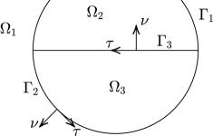
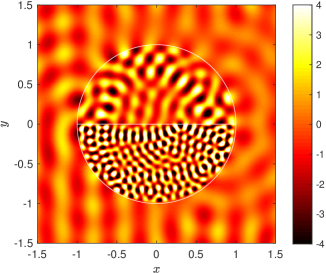
Figure 3: A three-region example. The vacuum wavenumber is $k_{0}=16$ and the relative permittivities are $\varepsilon_{1}=1$, $\varepsilon_{2}=4$, and $\varepsilon_{3}=16$. The incident field travels in the direction $d=(1,0)$. Left: the configuration. Right: $H_{z}(r,0)$ with colormap “hot” and a colorbar range restricted to $[-4,4]$, as in [10, Figure 4(a)].

We start with a three-region example from Jerez-Hanckes, Pérez-Arancibia, and Turc [10, Figure 4(a)]. The bounded object is a unit disk divided into two equisized regions, see Figure 3. The vacuum wavenumber is $k_{0}=16$ and the relative permittivities are $\varepsilon_{1}=1$, $\varepsilon_{2}=4$, and $\varepsilon_{3}=16$. The incident field travels in the direction $d=(1,0)$.

11.1.1 Numerical results for ${\boldsymbol{H}}$ and ${\boldsymbol{E}}$

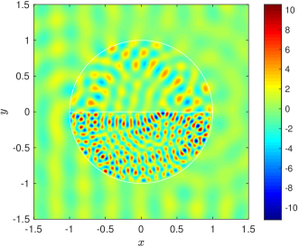
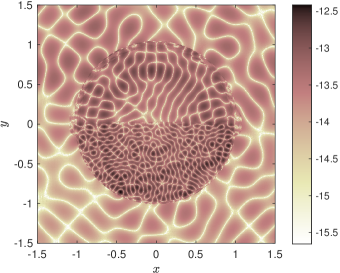
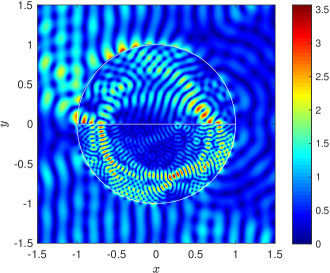
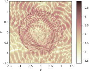
Figure 4: Numerical results for the three-region example in Figure 3. Top left: the field $H_{z}(r,0)$. Top right: $\log_{10}$ of estimated absolute field error in $H_{z}(r,0)$. Bottom left: the field $\lvert{\boldsymbol{E}}(r,0)\rvert$. Bottom right: $\log_{10}$ of estimated absolute field error in $\lvert{\boldsymbol{E}}(r,0)\rvert$.

The system (51) is solved using $1,\!696$ discretization points on the coarse mesh on $\Gamma$. Results for subsequent evaluations of the $z$-component of ${\boldsymbol{H}}(r,0)$ and of $\lvert{\boldsymbol{E}}(r,0)\rvert$ are shown in Figure 4. The local representations (35) and (56) are used for field points $r$ away from $\Gamma$ and the global representations (54) and (57) are used for field points $r$ close to $\Gamma$. We quote the following approximate timings: setting up the discretized system (51) took $7$ seconds, constructing various quantities needed in the RCIP scheme took $50$ seconds, solving the main linear system required $208$ GMRES iterations and took $3.5$ seconds. Computing ${\boldsymbol{H}}$ and ${\boldsymbol{E}}$ at $10^{6}$ field points placed on a Cartesian grid in the box ${\cal B}=\left\{-1.5\leq x\leq 1.5,-1.5\leq y\leq 1.5\right\}$ took, on average, $0.0011$ and $0.0022$ seconds per point, respectively.

11.1.2 Comparison with previous results for ${\boldsymbol{H}}$

The top left image of Figure 4 shows the field $H_{z}(r,0)$ using Matlab’s colormap “jet” and a colorbar range chosen as to include all values of $H_{z}(r,0)$ occurring in the box ${\cal B}$. For comparison with results in [10, Figure 4(a)], the right image of Figure 3 shows results with colormap “hot” and a colorbar range restricted to $[-4,4]$. A close comparison between the right image of Figure 3 and [10, Figure 4(a)] reveals that the figures look rather similar, except for at field points $r$ very close to $\Gamma$, where we think that our results are substantially more accurate than those of [10, Figure 4(a)].

11.1.3 Results for ${\boldsymbol{E}}$ via the extended representation

For comparison we also compute ${\boldsymbol{E}}(r,0)$ via the extended representation (63) rather than via (56) and (57). This involves augmenting the system of integral equations (51) with the extra equation (65). The estimated error in ${\boldsymbol{E}}(r,0)$ (not shown) is slightly improved by switching to the extended representation and resembles the error for $H_{z}(r,0)$ in the top right image of Figure 4. The timings were affected as follows: setting up the discretized augmented system (51) with (65) took $15$ seconds, constructing various quantities needed in the RCIP scheme took $75$ seconds, solving the main linear system required $233$ GMRES iterations and took $7$ seconds. Computing ${\boldsymbol{E}}(r,0)$ at $10^{6}$ field points $r$ in the box ${\cal B}$ took, on average, $0.0013$ seconds per point. That is, the system setup and solution take longer due to the extra unknown $\varrho_{\rm E}$, while the field evaluations are faster since we use the local representation (63) for all $r\in{\cal B}$ and avoid the expensive global representation (57) for $r$ close to $\Gamma$.

11.2 A four-region example

We now turn our attention to the four-region configuration of Figure 1. The object can be described as a unit disk centered at the origin and with two smaller disks of half the radius and origins at $x=\pm 1$ superimposed. The vacuum wavenumber is $k_{0}=10$ and the relative permittivities are $\varepsilon_{1}=1$, $\varepsilon_{2}=100$, and $\varepsilon_{3}=\varepsilon_{4}=625$. The incident field travels in the direction $d=(1,0)$. The example is inspired by the three-region high-contrast example of [5, Figure 5]

11.2.1 Numerical results for ${\boldsymbol{H}}$

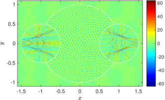
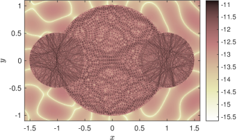
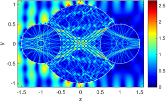
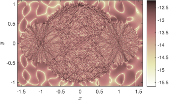
Figure 5: Results for the four-region example. The vacuum wavenumber is $k_{0}=10$ and the relative permittivities are $\varepsilon_{1}=1$, $\varepsilon_{2}=100$, and $\varepsilon_{3}=\varepsilon_{4}=625$. The incident field travels in the direction $d=(1,0)$. Top left: the field $H_{z}(r,0)$. Top right: $\log_{10}$ of estimated absolute field error in $H_{z}(r,0)$. Bottom left: the field $\lvert{\boldsymbol{E}}(r,0)\rvert$. Bottom right: $\log_{10}$ of estimated absolute field error in $\lvert{\boldsymbol{E}}(r,0)\rvert$.

The magnetic field is computed by first discretizing and solving the system (51) using $5,\!600$ discretization points on the coarse mesh on $\Gamma$ and then using (35) or (54) for field evaluations, depending on whether field points $r$ are far away from $\Gamma$ or not. In (51), we exclude parts of operators corresponding to (zero) contributions from surface densities on closed curves to subcurves that are separated in the sense of Section 8. Similarly, in (54), we exclude (zero) field contributions from layer potentials on closed curves that are distant to field points $r$. Numerical results are shown in the top row of Figure 5. Timings are as follows: setting up the discretized system (51) took $70$ seconds, constructing various quantities needed in the RCIP scheme took $50$ seconds, solving the main linear system required $596$ GMRES iterations and took $90$ seconds. Computing ${\boldsymbol{H}}$ at $1.455\times 10^{6}$ field points placed on a Cartesian grid in the box ${\cal B}=\left\{-1.6\leq x\leq 1.6,-1.1\leq y\leq 1.1\right\}$ took, on average, $0.0028$ seconds per point.

11.2.2 Numerical results for ${\boldsymbol{E}}$

When the dielectric contrast between the regions is high, the extended representation (63) of ${\boldsymbol{E}}$ offers better accuracy at field points $r$ very close to $\Gamma$ than do (56) and (57). Numerical results obtained with (63) and with $7,\!008$ discretization points on the coarse mesh on $\Gamma$ are shown in the bottom row of Figure 5. Timings are as follows: setting up the discretized system (51) with (65) took $125$ seconds, constructing various quantities needed in the RCIP scheme took $75$ seconds, solving the main linear system required $634$ GMRES iterations and took $300$ seconds. Computing ${\boldsymbol{E}}$ at the $1.455\times 10^{6}$ field points in ${\cal B}$ took, on average, $0.0043$ seconds per point.

11.2.3 A $20$ times triple-junction zoom for ${\boldsymbol{E}}$

We repeat the experiment of Section 11.2.2, zooming in on the subcurve triple junction at $\gamma_{1}=(-7/8,\sqrt{15}/8)\approx(-0.875,0.484)$ with a $20$ times magnification. This means that we evaluate ${\boldsymbol{E}}$ at $1.455\times 10^{6}$ field points in the box ${\cal B}\approx\left\{-0.955\leq x\leq-0.795,0.429\leq y\leq 0.539\right\}$.

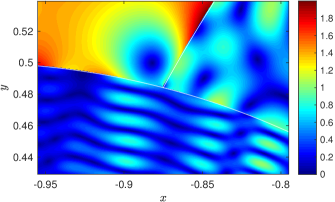
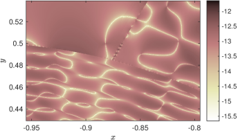
Figure 6: Same as the bottom row of Figure 5 but the computational box is now ${\cal B}\approx\left\{-0.955\leq x\leq-0.795,0.429\leq y\leq 0.539\right\}$.

The results, shown in Figure 6, illustrate that the extended representation (63), together with the other features in our numerical scheme, allow for high achievable accuracy for high-contrast problems also very close to subcurve triple junctions.

11.2.4 Convergence and asymptotic behavior

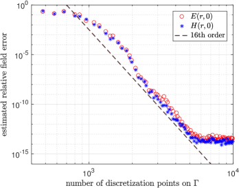
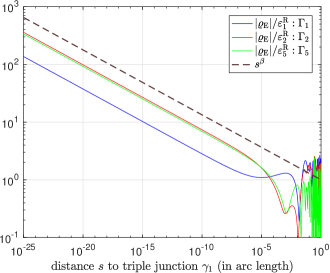
Figure 7: Left: convergence of $H_{z}(r,0)$ and $\lvert{\boldsymbol{E}}(r,0)\rvert$, shown in Figure 5, as a function of the number of discretization points used on the coarse mesh on $\Gamma$. Right: behavior of $\lvert\rho_{\rm E}(r)\rvert$ close to the subcurve triple junction $\gamma_{1}$ in Figure 6.

Our discretization scheme uses composite $16$-point Gauss–Legendre quadrature as underlying quadrature. If this was the only quadrature used, the overall convergence of the scheme would be $32$nd order. Since parts of the scheme rely on piecewise polynomial interpolation, however, the overall convergence is $16$th order. This is illustrated in the left image of Figure 7, where we show convergence for ${\boldsymbol{H}}(r,0)$ and ${\boldsymbol{E}}(r,0)$ with the number of discretization points used on the coarse mesh on $\Gamma$. The average estimated absolute field error is measured at $58,\!200$ points on a Cartesian grid in the box ${\cal B}=\left\{-1.6\leq x\leq 1.6,-1.1\leq y\leq 1.1\right\}$ and normalized with the largest field amplitude in ${\cal B}$. We use (35) or (54) for ${\boldsymbol{H}}(r,0)$ and (56) or (57) for ${\boldsymbol{E}}(r,0)$. The reason for not using the extended representation (63) of ${\boldsymbol{E}}(r,0)$ is that it is less memory efficient (in our present implementation) and that we need heavily overresolved reference solutions for some data points.

The RCIP method lends itself very well to accurate and fully automated asymptotic studies of surface densities close to singular boundary points, see [6, Section 14]. As an example we compute $\varrho_{\rm E}$ on $\Gamma_{1}$, $\Gamma_{2}$, and $\Gamma_{5}$ close to the subcurve triple junction $\gamma_{1}$, which is zoomed-in in Figure 6. The right image of Figure 7 shows $\lvert\varrho_{\rm E}(s)\rvert$ as a function of the distance $s$, in arclength, to $\gamma_{1}$. The leading asymptotic behavior is $\lvert\rho_{\rm E}(s)\rvert\propto s^{\beta}$, with $\beta=-0.1125730127414$, on all three subcurves.

11.3 Two-region examples under plasmonic conditions

We end this section by testing the new system (45). Recall that the system (45), with $c$ as in (46), has unique solutions on smooth $\Gamma$ when the conditions (47) hold. This includes plasmonic conditions. By this we mean that $k_{1}$ is real and positive and that the ratio $\varepsilon_{2}/\varepsilon_{1}$ is purely negative or, should no finite energy solution exist, arbitrarily close to and above the negative real axis. Under plasmonic conditions, and when $\Gamma$ has corners, so called surface plasmon waves can propagate along $\Gamma$. We will now revisit an example where this happens.

11.3.1 Surface plasmon waves

The example has $\Gamma$ given by [7, Eq. (93)], shown in Figure 2, and $k_{0}=18$, $\varepsilon_{1}=1$, $\varepsilon_{2}=-1.1838$, $c=-{\rm i}$, and $d=\left(\cos(\pi/4),\sin(\pi/4)\right)$. Results for $H_{z}^{+}(r,0)$ and $\nabla H_{z}^{+}(r,0)$, where the plus-sign superscript indicates a limit process for $\varepsilon_{2}/\varepsilon_{1}$, have been computed using an abstract-density approach from [12] in [7, Figure 7]. The main linear system in that approach has (50) as its system matrix, so the unique solvability is the same as for (45). The difference between the two approaches lies in the representation formulas they can use. The abstract-density approach is restricted to a local representation of $U$ [7, Eqs. (22) and (23)] which resembles (35) and exhibits stronger singularities as $\Omega_{n}\ni r\to r^{\prime}\in{\cal C}_{n}$ than does the global representation (54), which can be used only together with (45).

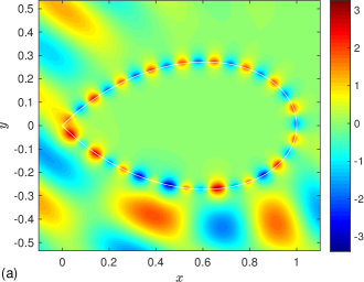
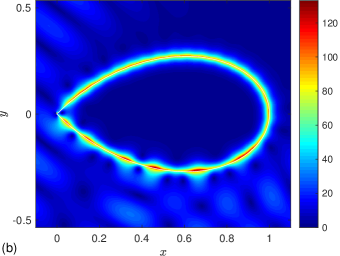
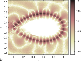
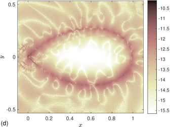
Figure 8: $H_{z}^{+}(r,0)$ and $\nabla H_{z}^{+}(r,0)$ with $k_{0}=18$, $\varepsilon_{1}=1$, $\varepsilon_{2}=-1.1838$, and $d=\left(\cos(\pi/4),\sin(\pi/4)\right)$: (a) The field $H_{z}^{+}(r,0)$; (b) The (diverging) field $\lvert\nabla H_{z}^{+}(r,0)\rvert$ with colorbar range set to $[0,133]$; (c) $\log_{10}$ of estimated absolute error in $H_{z}^{+}(r,0)$; (d) $\log_{10}$ of estimated absolute error in $\lvert\nabla H_{z}^{+}(r,0)\rvert$.

Figure 8 shows result obtained with the system (45) and the representations (35) and (54) and their gradients. There are $800$ discretization points on the coarse mesh on $\Gamma$ and $10^{6}$ field points on a rectangular Cartesian grid in the box ${\cal B}=\left\{-0.1\leq x\leq 1.1,-0.54\leq y\leq 0.54\right\}$. Comparing Figure 8 with [7, Figure 7], where the same grid was used, one can conclude that the achievable accuracy for $r$ close to $\Gamma$ is improved with around half a digit in $H_{z}^{+}(r,0)$ and one and a half digits in $\nabla H_{z}^{+}(r,0)$.

11.3.2 Unique solvability on the unit circle

In this last example, the statements made about unique solvability in Section 5.1 and Section 10 are illustrated by four simple examples on the unit circle. The setup is the same as in [7, Section 9.2], where the properties of (50) were studied: $\varepsilon_{1}=1$, $\varepsilon_{2}=-1.1838$, and the condition numbers of the systems under study are monitored as the vacuum wavenumber varies in the interval $k_{0}\in[0,10]$. A number of at least $20,\!000$ steps are taken in the sweeps and the stepsize is adaptively refined when sharp increases in the condition number are detected.

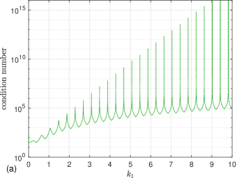
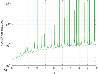
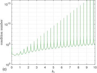
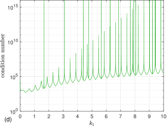
Figure 9: Condition numbers of system matrices on the unit circle, $\varepsilon_{2}/\varepsilon_{1}=-1.1838$, and $k_{1}\in[0,10]$: (a) the system (45) with $c=-{\rm i}\,$; (b) the Müller system; (c) the “${\boldsymbol{E}}$-system” with $c=-{\rm i}\,$; (d) the original “${\boldsymbol{E}}$-system”. The systems in (a,c) are free of false eigenwavenumbers while the systems in (b,d) exhibit twelve false eigenwavenumbers each.

We compare the system (45) with $c=-{\rm i}$, which is in agreement with (46), to the Müller system adapted to the problem of Section 2.2. The Müller system then corresponds to (45) with $c=-1.1838$, according to Section 10. Figure 9(a,b) shows that the system (45) with $c=-{\rm i}$ is uniquely solvable in this example while the Müller system has at least twelve wavenumbers $k_{1}=k_{0}\in[0,10]$ where it is not. A number of $384$ discretization points are used on $\Gamma$.

We also compare the two versions of the “${\boldsymbol{E}}$-system” [22, Eq. (37)], adapted to the problem of Section 2.2 and discussed in Section 10. Figure 9(c,d) shows that the “${\boldsymbol{E}}$-system” with $c=-{\rm i}$ in the modified representation (67) is uniquely solvable in this example while the original “${\boldsymbol{E}}$-system” with $c=-1.1838$ in (67) has the same twelve false eigenwavenumbers as the Müller system. A number of $768$ discretization points are used on $\Gamma$.

12 Conclusions

Using integral equation-based numerical techniques, we can solve planar multicomponent scattering problems for magnetic and electric fields with uniformly high accuracy in the entire computational domain. Almost all problems related to near-boundary field evaluations, redundant contributions from distant sources, and boundary subcurves meeting at triple junctions are gone. The success is achieved through new integral representations of electromagnetic fields in terms of physical surface densities, explicit kernel-split product integration, and the RCIP method.

References

- [1] M. Born and E. Wolf. Principles of optics: Electromagnetic theory of propagation, interference and diffraction of light. Pergamon Press, Oxford, third edition, 1965.
- [2] X. Claeys and R. Hiptmair. Multi-trace boundary integral formulation for acoustic scattering by composite structures. Comm. Pure Appl. Math., 66(8):1163–1201, 2013.
- [3] D. Colton and R. Kress. Integral equation methods in scattering theory. Pure and Applied Mathematics. John Wiley & Sons, Inc., New York, 1983.
- [4] D. Colton and R. Kress. Inverse acoustic and electromagnetic scattering theory, volume 93 of Applied Mathematical Sciences. Springer-Verlag, Berlin, second edition, 1998.
- [5] L. Greengard and J.-Y. Lee. Stable and accurate integral equation methods for scattering problems with multiple material interfaces in two dimensions. J. Comput. Phys., 231(6):2389–2395, 2012.
- [6] J. Helsing. Solving integral equations on piecewise smooth boundaries using the RCIP method: a tutorial. arXiv:1207.6737v9 [physics.comp-ph], revised 2018.
- [7] J. Helsing and A. Karlsson. On a Helmholtz transmission problem in planar domains with corners. J. Comput. Phys., 371:315–332, 2018.
- [8] J. Helsing and R. Ojala. On the evaluation of layer potentials close to their sources. J. Comput. Phys., 227(5):2899–2921, 2008.
- [9] J. Helsing and R. Ojala. Elastostatic computations on aggregates of grains with sharp interfaces, corners, and triple-junctions. Int. J. Solids. Struct., 46(25):4437–4450, 2009.
- [10] C. Jerez-Hanckes, C. Pérez-Arancibia, and C. Turc. Multitrace/singletrace formulations and domain decomposition methods for the solution of Helmholtz transmission problems for bounded composite scatterers. J. Comput. Phys., 350:343–360, 2017.
- [11] A. Kirsch and F. Hettlich. The mathematical theory of time-harmonic Maxwell’s equations, volume 190 of Applied Mathematical Sciences. Springer, Cham, 2015.
- [12] R.E. Kleinman and P.A. Martin. On single integral equations for the transmission problem of acoustics. SIAM J. Appl. Math., 48(2):307–325, 1988.
- [13] R.E. Kleinman, G.F. Roach, and S.E.G. Ström. The null field method and modified Green functions. Proc. Roy. Soc. London Ser. A, 394(1806):121–136, 1984.
- [14] R. Kress. On the numerical solution of a hypersingular integral equation in scattering theory. J. Comput. Appl. Math., 61(3):345–360, 1995.
- [15] R. Kress and G.F. Roach. Transmission problems for the Helmholtz equation. J. Math. Phys., 19(6):1433–1437, 1978.
- [16] G. Kristensson. Scattering of electromagnetic waves by obstacles. Mario Boella Series on Electromagnetism in Information and Communication. SciTech Publishing, an imprint of the IET, Edison, NJ, 2016.
- [17] J. Lai and S. Jiang. Second kind integral equation formulation for the mode calculation of optical waveguides. Appl. Comput. Harmon. Anal., 44(3):645–664, 2018.
- [18] P.A. Martin. On the null-field equations for the exterior problems of acoustics. Quart. J. Mech. Appl. Math., 33(4):385–396, 1980.
- [19] J.R. Mautz and R.F. Harrington. Electromagnetic scattering from a homogeneous body of revolution. Technical Report No. TR-77-10, Deptartment of electrical and computer engineering, Syracuse University, New York, 1977.
- [20] C. Müller. Foundations of the mathematical theory of electromagnetic waves. Revised and enlarged translation from the German. Die Grundlehren der mathematischen Wissenschaften, Band 155. Springer-Verlag, Berlin, 1969.
- [21] S. Ström. On the integral equations for electromagnetic scattering. Am. J. Phys., 43(12):1060–1069, 1975.
- [22] F. Vico, L. Greengard, and M. Ferrando. Decoupled field integral equations for electromagnetic scattering from homogeneous penetrable obstacles. Comm. Part. Differ. Equat., 43(2):159–184, 2018.
- [23] P.C. Waterman. Matrix formulation of electromagnetic scattering. Proc. IEEE, 53(8):805–812, 1965.