On-Demand Generation of Traveling Cat States Using a Parametric Oscillator

Abstract

We theoretically propose a method for on-demand generation of traveling Schrödinger cat states, namely, quantum superpositions of distinct coherent states of traveling fields. This method is based on deterministic generation of intracavity cat states using a Kerr-nonlinear parametric oscillator (KPO) via quantum adiabatic evolution. We show that the cat states generated inside a KPO can be released into an output mode by controlling the parametric pump amplitude dynamically. We further show that the quality of the traveling cat states can be improved by using a shortcut-to-adiabaticity technique.

I Introduction

Quantum superposition is one of the most strange and intriguing concepts in quantum mechanics and a useful resource for quantum information processing. Superpositions of macroscopically distinct states are often referred to as Schrödinger cat states, or cat states for short, named after Schrödinger’s famous gedankenexperiment with a cat in a superposition of alive and dead states Haroche2013a ; Wineland2013a . In quantum optics, superpositions of distinct coherent states are called cat states Leonhardt , because coherent states are often regarded as the “most classical” states of light.

Such cat states have been generated experimentally by various approaches. In the optical regime, cat states of small size, which are sometimes called Schrödinger kittens, have been generated by subtracting one photon from squeezed states of light Ourjoumtsev2006a ; Wakui2007a . Optical cat states of a little larger size have been generated by other methods Ourjoumtsev2007a ; Sychev2017a . Note that these optical cat states are of traveling fields and generated probabilistically.

In the microwave regime, cat states of larger size have been generated experimentally Deleglise2008a ; Vlastakis2013a ; Leghtas2015a ; Touzard2018a . The generation using Rydberg atoms Deleglise2008a is heralded by measurement results of the atomic states, where the parity, ‘even’ or ‘odd’, of the cat state is determined randomly according to the measurement results. On-demand generations of microwave cat states have been demonstrated using superconducting circuits by two different approaches, one of which is based on conditional operations using a superconducting quantum bit (qubit) Vlastakis2013a and the other is based on two-photon driving and two-photon loss larger than one-photon loss Leghtas2015a ; Touzard2018a . By extending the former approach to a two-cavity case, entangled coherent states in two cavities have been observed experimentally Wang2016a . Note that these microwave cat states are confined inside cavities. Recently, the cat state generated inside a cavity has been released by controlling the output coupling rate of the cavity using four-wave mixing in the qubit Pfaff2017a . To the best of our knowledge, only this experiment has demonstrated on-demand generation of traveling cat states.

In this paper, we propose a simple alternative method for on-demand generation of traveling cat states. Our method is based on a recent theoretical result that a Kerr-nonlinear parametric oscillator (KPO) can generate intracavity cat states deterministically via quantum adiabatic evolution Goto2016a ; Puri2017a . (The KPO has recently attracted attention for its application to quantum computing Goto2016a ; Puri2017a ; Goto2016b ; Nigg2017a ; Puri2017b .) In the previous work, the KPO is assumed to be lossless in ideal cases, and therefore the cat states are confined inside the KPO. In the present work, we theoretically investigate a coupled system of a KPO and a one-dimensional system (output mode). It turns out that the cat states generated inside a KPO can be released into the output mode by controlling the parametric pump amplitude dynamically, while the output coupling rate is constant. Hence by using a KPO, we can generate traveling cat states on demand without controlling the output coupling rate.

II Model

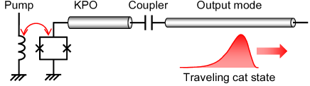
Figure 1: Coupled system of a KPO and an output mode. The KPO is implemented by a Josephson parametric oscillator (JPO) Lin2014a with a relatively large Kerr effect. The JPO is capacitively coupled to a transmission line for the output mode. Traveling cat state is generated by controlling the pump field dynamically.

The coupled system of a KPO and an output mode is depicted in Fig. 1, where a superconducting-circuit implementation is supposed Nigg2017a ; Puri2017b ; Lin2014a . In a frame rotating at half the pump frequency, $\omega_{p}/2$, of the parametric pumping and in the rotating-wave approximation, the system is modeled by the following Hamiltonian Goto2016a ; Puri2017a ; Gardiner1985a ; Milburn ; Duan2003a ; Goto2005a (we use the units $\hbar=v_{p}=1$, where $v_{p}$ is the phase velocity of the electromagnetic fields in the output mode):

$$H(t) =H_{\mathrm{KPO}}(t)+H_{\mathrm{out}}+H_{c},$$ (1)

$$H_{\mathrm{KPO}}(t) =\frac{p(t)}{2}\left(a^{\dagger 2}+a^{2}\right)-\frac{K}{2}a^{\dagger 2}a^{2}+\Delta a^{\dagger}a,$$ (2)

$$H_{\mathrm{out}} =\int_{-\infty}^{\infty}\!\omega b^{\dagger}(\omega)b(\omega)\,d\omega,$$ (3)

$$H_{c} =i\sqrt{\frac{\kappa_{\mathrm{ex}}}{2\pi}}\int_{-\infty}^{\infty}\!\left[b^{\dagger}(\omega)a-a^{\dagger}b(\omega)\right]d\omega,$$ (4)

where $a^{\dagger}$ and $a$ are the creation and annihilation operators for the KPO, $p(t)$ is the time-dependent pump amplitude, $K$ is the magnitude of the Kerr coefficient comment-Kerr , $\Delta=\omega_{\mathrm{KPO}}-\omega_{p}/2$ is the detuning frequency ($\omega_{\mathrm{KPO}}$ is the one-photon resonance frequency of the KPO), $b^{\dagger}(\omega)$ and $b(\omega)$ are the creation and annihilation operators for photons of frequency (or wave number) $\omega_{p}/2+\omega$ in the output mode, and $\kappa_{\mathrm{ex}}$ is the energy decay rate of the KPO due to its coupling to the output mode. Here we assume no internal loss of the KPO, which is discussed later. Hereafter, we consider the resonance case ($\Delta=0$).

If the KPO is a closed system (${\kappa_{\mathrm{ex}}=0}$), a cat state ${|\alpha_{0}\rangle+|{-\alpha_{0}}\rangle}$ can be generated from the vacuum state $|0\rangle$ via quantum adiabatic evolution by gradually increasing $p(t)$ from zero to ${p_{0}=K\alpha_{0}^{2}}$ Goto2016a ; Puri2017a . When the KPO is coupled to the output mode, the photons inside the KPO will leak to the output mode. As a result, the entanglement between the KPO and the output mode arises during the generation. Moreover, the decay of the KPO due to the leak may degrade the adiabatic cat-state generation. Thus, it is not obvious whether or not we can generate a traveling cat state using the KPO.

III Proposed method

Our idea is based on the fact that any quantum state inside a linear cavity results in a traveling pulse in the same quantum state through the leak to the output mode, where the pulse shape is exponential corresponding to the exponential decay Eichler2011a . This property of linear cavities removes the concern with the entanglement. The issue with the decay can also be solved by generating a cat state faster than the decay, which is possible if $K$ is much larger than $\kappa_{\mathrm{ex}}$. The remaining problem is that the KPO has a large Kerr effect, namely, it is not a linear cavity.

Our solution is to switch off the parametric pumping as ${p(t)\propto\exp(-\kappa_{\mathrm{ex}}t)}$ after the cat-state preparation. Then the Kerr term and the pumping term are cancelled out each other, and hence the KPO can be regarded as a linear cavity. This is confirmed as follows. Suppose that at time $t_{0}$, the KPO is prepared in a cat state ${|\alpha_{0}\rangle+|{-\alpha_{0}}\rangle}$, where $\displaystyle{\alpha_{0}=\sqrt{p_{0}/K}}$ and ${p_{0}=p(t_{0})}$. Since $H_{\mathrm{KPO}}(t)$ in Eq. (2) is rewritten as $\displaystyle{H_{\mathrm{KPO}}(t)=-\frac{K}{2}\!\left(a^{\dagger 2}-\frac{p(t)}{K}\right)\!\left(a^{2}-\frac{p(t)}{K}\right)}$ by dropping a c-number term, ${H_{\mathrm{KPO}}(t_{0})|{\pm\alpha_{0}}\rangle\propto\alpha_{0}^{2}-p_{0}/K=0}$, where ${a|{\pm\alpha_{0}}\rangle=\pm\alpha_{0}|{\pm\alpha_{0}}\rangle}$ Leonhardt . Thus at $t_{0}$, the amplitude starts decreasing as $\displaystyle{\pm\alpha(t)=\pm\alpha_{0}e^{-\kappa_{\tiny{\mbox{ex}}}(t-t_{0})/2}}$ because of the external coupling. If we set the pump amplitude as $p(t)=p_{0}e^{-\kappa_{\tiny{\mbox{ex}}}(t-t_{0})}$, $H_{\mathrm{KPO}}(t)|{\pm\alpha(t)}\rangle\propto\alpha(t)^{2}-p(t)/K=0$, that is, the Kerr term and the pumping term are cancelled out at any time $t\geq t_{0}$. Thus, the KPO behaves like a linear cavity during the release of the cat state, and therefore the cat state prepared inside the KPO is faithfully released as a traveling cat state.

IV Numerical simulation

To examine the above method quantitatively, we numerically solve the Schrödinger equation with the Hamiltonian in Eq. (1) and evaluate the fidelity between the output pulse and an ideal cat state. An approach to the numerical simulation is based on the discretization of frequency $\omega$ (or wave number $\omega/v_{p}$) Duan2003a ; Goto2005a . In the present case, however, the photon number in the one-dimensional system is larger than one, and consequently such discretization results in a complicated system of differential equations. In this work, we instead discretize the position, which results in simpler equations as shown below.

We first introduce the annihilation operator with respect to the position $z$:

$$\tilde{b}(z) =\frac{1}{\sqrt{2\pi}}\int_{-\infty}^{\infty}\!b(\omega)e^{i\omega z}\,d\omega.$$ (5)

Then, we move to the interaction picture with the unitary operator $U(t)=e^{-iH_{\mathrm{out}}t}$ as follows:

$$\tilde{b}_{I}(z,t) =U^{\dagger}(t)\tilde{b}(z)U(t)=\tilde{b}(z-t),$$

$$H_{I}(t) =U^{\dagger}(t)\left[H_{\mathrm{KPO}}(t)+H_{c}\right]U(t)$$

$$=H_{\mathrm{KPO}}(t)+i\sqrt{\kappa_{\mathrm{ex}}}\left[\tilde{b}^{\dagger}(-t)a-a^{\dagger}\tilde{b}(-t)\right].$$

A pulse-mode operator for the interval $[0,T]$ is defined as

$$b_{p}=\int_{0}^{T}\!f_{p}(z)\tilde{b}_{I}(z,T)\,dz=\int_{0}^{T}\!f_{p}(T-z)\tilde{b}(-z)\,dz,$$

where $f_{p}(z)$ is the normalized envelope function for the output pulse satisfying $\displaystyle\int_{0}^{T}\!|f_{p}(z)|^{2}dz=1$. In the present work, we define $f_{p}(z)$ as ${f_{p}(z)\propto\sqrt{\langle\tilde{b}^{\dagger}_{I}(z,T)\tilde{b}_{I}(z,T)\rangle}}$, where $\langle\tilde{b}^{\dagger}_{I}(z,T)\tilde{b}_{I}(z,T)\rangle$ is the spatial distribution of photons in the output mode at the final time $T$. Note that in experiments, we can find such $f_{p}(z)$ from the measurement of the output power from the KPO.

Next, we divide the interval $[0,T]$ into $J$ small intervals $[z_{j-1},z_{j}]$ ($j=1,2,\ldots,J$), where the intervals $\Delta z_{j}=z_{j}-z_{j-1}$ are set to small values supplement . Then, $\tilde{b}(z)$ and $f_{p}(z)$ are discretized as follows ($z\in[z_{j-1},z_{j}]$):

$$\tilde{b}(-z)\sqrt{\Delta z_{j}}\to\tilde{b}_{j},~{}f_{p}(T-z)\sqrt{\Delta z_{j}}\to f_{j}.$$ (6)

Then, the commutation relation $[\tilde{b}(z),\tilde{b}^{\dagger}(z^{\prime})]=\delta(z-z^{\prime})$ becomes $[\tilde{b}_{j},\tilde{b}^{\dagger}_{l}]=\delta_{j,l}$ and the normalization condition $\displaystyle\int_{0}^{T}\!|f_{p}(z)|^{2}dz=1$ becomes $\displaystyle\sum_{j=1}^{J}|f_{j}|^{2}=1$. By transforming the integration with respect to $z$ to the summation with respect to $j$, we obtain

$$b_{p}=\sum_{j=1}^{J}f_{j}\tilde{b}_{j},~{}f_{j}=\sqrt{\frac{\langle\tilde{b}_{j}^{\dagger}\tilde{b}_{j}\rangle}{\sum_{l=1}^{J}\langle\tilde{b}_{l}^{\dagger}\tilde{b}_{l}\rangle}}.$$ (7)

The Hamiltonian at time $t\in[z_{j-1},z_{j}]$ is given by

$$H_{I}(t) =H_{\mathrm{KPO}}(t)+i\sqrt{\kappa_{\mathrm{ex}}}\left[\tilde{b}_{j}^{\dagger}a-a^{\dagger}\tilde{b}_{j}\right].$$ (8)

We numerically solve the Schrödinger equation with the Hamiltonian in Eq. (8) supplement . Since the Hamiltonian includes only one of $\{\tilde{b}_{j}\}$, the corresponding Schrödinger equation is simple. In the present work, we investigate the cases where $\kappa_{\mathrm{ex}}=0.2K$.

As explained above, $p(t)$ should satisfy the following two conditions: $p(t)$ is increased fast enough to adiabatically generate a cat state inside the KPO before the decay spoils it; after that, $p(t)$ is decreased as $\displaystyle{p(t)\propto\exp(-\kappa_{\mathrm{ex}}t)}$ so that the Kerr term and the pumping term are cancelled out. To satisfy these conditions simultaneously, we define $p(t)$ as the output of the fourth order low-pass filter (LPF) supplement ; Wiseman with the input ${p_{\mathrm{in}}(t)=KA_{p}\exp(-\kappa_{\mathrm{ex}}t)}$. The dimensionless parameter $A_{p}$ is used for tuning the photon number of the traveling cat state. We set the photon number to about 2, which is large enough for the two coherent states being distinct but small enough to solve the Schrödinger equation numerically. The bandwidth, $B$, of the LPF supplement ; Wiseman is set to $B=0.5K$ between $\kappa_{\mathrm{ex}}$ and $K$. The final time $T$ is set such that the final photon number, $n_{\mathrm{in}}$, in the KPO is less than $10^{-3}$ (see Table 1).

We obtain the density operator, $\rho$, describing the quantum state of the output pulse using the moments $M_{m,n}=\langle b_{p}^{\dagger m}b_{p}^{n}\rangle$ with $b_{p}$ in Eq. (7). The density matrix with respect to the Fock states is given by the following formula Eichler2012a :

$$\rho_{m,n}=\frac{1}{\sqrt{m!n!}}\sum_{l=0}^{\infty}\frac{(-1)^{l}}{l!}M_{n+l,m+l}.$$ (9)

Using the density matrix, we calculate the corresponding Wigner function $\displaystyle{W(\beta)=\frac{2}{\pi}\mbox{Tr}\!\left[D(-\beta)\rho D(\beta)P\right]}$ Leonhardt ; Deleglise2008a ; Goto2016a , where $\displaystyle{D(\beta)=\exp\!\left(\beta b_{p}^{\dagger}-\beta^{*}b_{p}\right)}$ (the asterisk denotes complex conjugation) and $\displaystyle{P=\exp\!\left(i\pi b_{p}^{\dagger}b_{p}\right)}$.

The results of the numerical simulation are shown in Fig. 2(a) and the first row of Table 1. Table 1 also provides the setting of the simulation. Figure 2(a) shows that the photon number in the KPO varies in a similar manner to the pump amplitude, as expected. The Wigner function for the output pulse in Fig. 2(a) clearly shows the interference fringe, which is the evidence for the quantum superposition of the two coherent states, that is, the output pulse is in a cat state. (The tilt of the Wigner function, which corresponds to $\theta_{\mathrm{cat}}$ in Table 1, is due to the residual Kerr effect.) As shown in Table 1, the maximum fidelity between this output state and an ideal cat state is 0.962. Thus, the present method works successfully as expected.

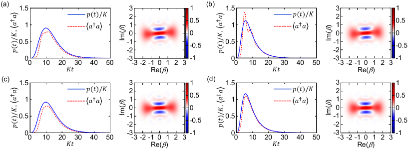
Figure 2: Simulation results of traveling cat-state generation using a KPO. Left: Time evolutions of the pump amplitude $p(t)$ and the expectation value of the photon number, $\langle a^{\dagger}a\rangle$, in the KPO. Right: Wigner function, $W(\beta)$, of the output pulse. See Table 1 for the settings of (a)–(d).

Table 1: Results and setting of numerical simulations. Fidelity: maximum fidelity between the output state and the ideal cat state with two parameters: $\displaystyle(|\beta_{\mathrm{cat}}e^{i\theta_{\tiny{\mbox{cat}}}}\rangle+|{-\beta_{\mathrm{cat}}e^{i\theta_{\tiny{\mbox{cat}}}}}\rangle)/\sqrt{2(1+e^{-2\beta_{\tiny{\mbox{cat}}}^{2}})}$, where $\beta_{\mathrm{cat}}$ and $\theta_{\mathrm{cat}}$ are the magnitude and phase of the cat-state amplitude, respectively. $\beta_{\mathrm{cat}}^{2}$ and $\theta_{\mathrm{cat}}/\pi$: values maximizing the fidelity. $\beta_{\mathrm{cat}}^{2}$ is close to 2, which means that the photon number of the output pulse is about 2. $n_{\mathrm{in}}$: average photon number in the KPO at the final time $T$. $I_{t}$: time integral of the average photon number in the KPO, that is, $I_{t}=\int_{0}^{T}\!\langle a^{\dagger}a\rangle\,dt$. In all the cases, ${I_{t}\approx 10K^{-1}=2\kappa_{\mathrm{ex}}^{-1}}$, because ${\kappa_{\mathrm{ex}}I_{t}}$ corresponds to the photon number of the output pulse.

	Fidelity	$~{}~{}\beta_{\mathrm{cat}}^{2}~{}~{}$	$~{}~{}\theta_{\mathrm{cat}}/\pi~{}~{}$	$n_{\mathrm{in}}$	$~{}~{}KI_{t}~{}~{}$	Shortcut	$~{}~{}\kappa_{\mathrm{ex}}/K~{}~{}$	$~{}~{}B/K~{}~{}$	$~{}~{}A_{p}~{}~{}$	$~{}~{}KT~{}~{}$	$~{}~{}J~{}~{}$
Fig. 2(a)	0.962	2.01	0.03	$6.2\times 10^{-4}$	9.63	Unused	0.2	0.5	2.45	50	80
Fig. 2(b)	0.930	1.96	0.02	$6.1\times 10^{-4}$	9.64	Unused	0.2	1.0	2.15	45	80
Fig. 2(c)	0.983	2.03	0.02	$6.4\times 10^{-4}$	9.63	Used	0.2	0.5	2.50	50	80
Fig. 2(d)	0.993	2.02	0.01	$6.4\times 10^{-4}$	9.60	Used	0.2	1.0	2.25	45	80

V Improvement by shortcut to adiabaticity

The imperfection of the generated traveling cat state may be partially due to the leak during the initial cat-state preparation. We can speed up the preparation by setting the LPF bandwidth $B$ to a larger value, e.g., $B=K$. Then, however, nonadiabatic effects degrade the cat state. The simulation results for $B=K$ are shown in Fig. 2(b) and the second row of Table 1. The oscillation of $\langle a^{\dagger}a\rangle$ in Fig. 2(b) is due to the nonadiabatic effects. Consequently, the maximum fidelity between the output state and an ideal cat state decreases to 0.930 (see Table 1).

To mitigate the nonadiabatic effects, we can use the technique called shortcut to adiabaticity Puri2017a ; Demirplak2003a ; Campo2013a . To maintain quantum adiabatic evolution, the shortcut-to-adiabaticity technique introduces the following counterdiabatic Hamiltonian Demirplak2003a ; Campo2013a :

$$H_{\mathrm{counter}}=i\sum_{n}|\dot{\phi}_{n}\rangle\langle\phi_{n}|,$$ (10)

where $|\phi_{n}\rangle$ is the $n$-th instantaneous eigenstate of the slowly varying Hamiltonian and the dot denotes the time derivative.

In the present case, the counterdiabatic Hamiltonian is approximately given by supplement ; comment-shortcut

$$H_{\mathrm{counter}}(t) =i\frac{p^{\prime}(t)}{2}\left(a^{\dagger 2}-a^{2}\right),$$ (11)

$$p^{\prime}(t) =\frac{\dot{p}(t)}{p(t)}\tanh\!\frac{p(t)}{K}.$$ (12)

The physical meaning of the counterdiabatic Hamiltonian is to add the imaginary pump amplitude $p^{\prime}(t)$ to the real one $p(t)$. This is experimentally possible by controlling the phase of the pump field.

The simulation results with the shortcut-to-adiabaticity technique are shown in Figs. 2(c) and 2(d) and the third and fourth rows of Table 1. As shown in Fig. 2(d), the oscillation of $\langle a^{\dagger}a\rangle$ does not occur even when $B=K$, unlike Fig. 2(b). This demonstrates that the shortcut-to-adiabaticity technique works successfully. The fidelity is improved for both $B=0.5K$ and $K$. Contrary to the results without the shortcut-to-adiabaticity technique, the fidelity is higher for larger $B$, and the corresponding infidelity is lower than 1% when $B=K$ (See Table 1). Thus, the shortcut-to-adiabaticity technique can significantly improve the quality of the traveling cat state.

VI Internal loss

So far, internal loss of the KPO has not been taken into account. However, any actual devices have internal loss, and it degrades the coherence of the cat states. Here we briefly examine the effect of the internal loss in the superconducting-circuit implementation of the KPO Nigg2017a ; Puri2017b ; Lin2014a .

Assuming that $K/(2\pi)=10$ MHz and $\omega_{\mathrm{KPO}}/(2\pi)=10$ GHz as typical values, $\kappa_{\mathrm{ex}}=0.2K$ in the present simulations corresponds to the external quality factor, $Q_{\mathrm{ex}}=\omega_{\mathrm{KPO}}/\kappa_{\mathrm{ex}}$, of $5\times 10^{3}$. On the other hand, the probability of losing a photon inside the KPO, which gives an upper bound on the infidelity due to the internal loss, is approximately given by $\kappa_{\mathrm{in}}I_{t}$, where $\kappa_{\mathrm{in}}$ is the internal-loss rate and ${I_{t}=\int_{0}^{T}\!\langle a^{\dagger}a\rangle\,dt}$. In Table 1, ${I_{t}\approx 10K^{-1}=2\kappa_{\mathrm{ex}}^{-1}}$ in all the cases. Thus, in order to have an intra-KPO photon-loss probability below, e.g., 10%, the required condition is $\kappa_{\mathrm{in}}I_{t}\approx 10\kappa_{\mathrm{in}}/K\leq 0.1$, which is equivalent to the internal quality factor of $Q_{\mathrm{in}}\geq 10^{5}$. These values of $Q_{\mathrm{ex}}$ and $Q_{\mathrm{in}}$ seem feasible with current technologies.

VII Conclusion

We have shown that the cat states deterministically generated inside a KPO via quantum adiabatic evolution can be released into an output mode by controlling the pump amplitude properly. Thus, on-demand generation of traveling cat states can be realized using a KPO. We have further shown that a shortcut-to-adiabaticity technique, where the phase of the pump field is controlled dynamically in time, can improve the quality of the traveling cat state significantly. The traveling cat states generated by a KPO can be directly observed by, e.g., homodyne or heterodyne detection of the output field. Thus, this can be used for experimentally demonstrating the ability of a KPO to generate cat states deterministically.

Appendix A Numerical simulation method

In the simulation presented in the main text, we truncate the photon number in the output mode at 6, which is sufficiently large to express a cat state with average photon number of 2. Then, the state vector $|\psi\rangle$ describing the coupled system is represented as follows:

$$|\psi\rangle =\sum_{n=0}^{N_{0}}\psi_{0}(n)|n\rangle|0\rangle+\sum_{n=0}^{N_{1}}\sum_{j_{1}=1}^{J}\psi_{1}(n,j_{1})|n\rangle|j_{1}\rangle+\sum_{n=0}^{N_{2}}\sum_{j_{1}=1}^{J}\sum_{j_{2}=1}^{j_{1}}\psi_{2}(n,j_{1},j_{2})|n\rangle|j_{1},j_{2}\rangle$$

$$+\sum_{n=0}^{N_{3}}\sum_{j_{1}=1}^{J}\sum_{j_{2}=1}^{j_{1}}\sum_{j_{3}=1}^{j_{2}}\psi_{3}(n,j_{1},j_{2},j_{3})|n\rangle|j_{1},j_{2},j_{3}\rangle+\sum_{n=0}^{N_{4}}\sum_{j_{1}=1}^{J}\sum_{j_{2}=1}^{j_{1}}\sum_{j_{3}=1}^{j_{2}}\sum_{j_{4}=1}^{j_{3}}\psi_{4}(n,j_{1},j_{2},j_{3},j_{4})|n\rangle|j_{1},j_{2},j_{3},j_{4}\rangle$$

$$+\sum_{n=0}^{N_{5}}\sum_{j_{1}=1}^{J}\sum_{j_{2}=1}^{j_{1}}\sum_{j_{3}=1}^{j_{2}}\sum_{j_{4}=1}^{j_{3}}\sum_{j_{5}=1}^{j_{4}}\psi_{5}(n,j_{1},j_{2},j_{3},j_{4},j_{5})|n\rangle|j_{1},j_{2},j_{3},j_{4},j_{5}\rangle$$

$$+\sum_{n=0}^{N_{6}}\sum_{j_{1}=1}^{J}\sum_{j_{2}=1}^{j_{1}}\sum_{j_{3}=1}^{j_{2}}\sum_{j_{4}=1}^{j_{3}}\sum_{j_{5}=1}^{j_{4}}\sum_{j_{6}=1}^{j_{5}}\psi_{6}(n,j_{1},j_{2},j_{3},j_{4},j_{5},j_{6})|n\rangle|j_{1},j_{2},j_{3},j_{4},j_{5},j_{6}\rangle,$$ (13)

where the first and second ket vectors represent the Fock states of the KPO and the output mode, respectively, and $N_{l}$ ($l=0,1,\ldots,6$) is the number at which the photon number in the KPO is truncated when the photon number in the output mode is $l$. In the present simulations, we set $N_{0}=N_{1}=N_{2}=6$, $N_{3}=5$, $N_{4}=4$, $N_{5}=3$, and $N_{6}=2$. The second ket vector is defined with the creation operators, e.g., as follows:

$$|j_{1},j_{2},j_{3}\rangle=\mathcal{N}(j_{1},j_{2},j_{3})\tilde{b}^{\dagger}_{j_{1}}\tilde{b}^{\dagger}_{j_{2}}\tilde{b}^{\dagger}_{j_{3}}|0\rangle,$$ (14)

where the normalization factor $\mathcal{N}$ is defined as

$$\mathcal{N}(j_{1},j_{2},j_{3})=\left\{\begin{matrix}1&\cdots&j_{1}>j_{2}>j_{3},\\ 1/\sqrt{2!}&\cdots&j_{1}=j_{2}>j_{3},\\ 1/\sqrt{2!}&\cdots&j_{1}>j_{2}=j_{3},\\ 1/\sqrt{3!}&\cdots&j_{1}=j_{2}=j_{3}.\\ \end{matrix}\right.$$ (15)

Using this representation, we numerically solved the Schrödinger equation with the Hamiltonian in Eq. (8) in the main text. Since the Hamiltonian includes only one of $\{\tilde{b}_{j}\}$, the corresponding Schrödinger equation is simple. Moreover, at time $t\in[z_{j-1},z_{j}]$, $|\psi\rangle$ includes only the output-mode photons satisfying $j_{1}\leq j$ in Eq. (13). This enables fast implementation of the simulation.

Since the photon number in the KPO is large (small) in the first (second) half of the whole process, we set correspondingly the intervals $\Delta z_{j}$ to small (large) values. More concretely, we set $\Delta z_{j}=(T/2)/(4J/5)$ for $j=1,2,\cdots,4J/5$ and $\Delta z_{j}=(T/2)/(J/5)$ for $j=4J/5+1,4J/5+2,\cdots,J$. (So we set $J$ to multiples of 5.) We use the fourth-order Runge-Kutta method for numerically solving the Schrödinger equation, where the time steps are set to about $0.1K^{-1}$. These time steps are defined by dividing $\Delta z_{j}$ by appropriate integers.

As mentioned in the main text, We set $J=80$ in the present simulations. The following results show that this value of $J$ is sufficiently large. Figure 3 shows the $J$ dependence of the final photon number, $n_{\mathrm{out}}=\sum_{j=1}^{J}\langle\tilde{b}_{j}^{\dagger}\tilde{b}_{j}\rangle$, in the output mode. These data, the circles in Fig. 3, are well fitted with $n_{0}-b/J$, the solid lines in Fig. 3, where $n_{0}$ and $b$ are the fitting parameters. This is natural because the position discretization is the first-order approximation with respect to $J^{-1}$. The dashed lines in Fig. 3 show $n_{\mathrm{out}}=n_{0}$, which are the estimated values of $n_{\mathrm{out}}$ in the limit $J\to\infty$. From the small discrepancies between the data and $n_{0}$, indicated by arrows in Fig. 3, the numerical errors due to finite $J$ are estimated to be less than 1%. This indicates that $J$ is sufficiently large.

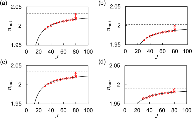
Figure 3: $J$ dependence of the final photon number, $n_{\mathrm{out}}=\sum_{j=1}^{J}\langle\tilde{b}_{j}^{\dagger}\tilde{b}_{j}\rangle$, in the output mode. (a)–(d) correspond to Figs. 2(a)–2(d), respectively, in the main text. Circles represent simulation results. Solid lines are fitted curves with $n_{\mathrm{out}}(J)=n_{0}-b/J$, where $n_{0}$ and $b$ are the fitting parameters. Horizontal dashed lines represent $n_{\mathrm{out}}(J)=n_{0}$. Arrows indicate the discrepancies between the data and $n_{0}$.

Appendix B Pulse shape control using low-pass filters

In the simulation presented in the main text, we define the pulse shape of the pump amplitude $p(t)$ as the output of the fourth-order low-pass filter (LPF) [29] with the input ${p_{\mathrm{in}}(t)=KA_{p}\exp(-\kappa_{\scriptsize{\mbox{ex}}}t)}$. The input-output relation of a LPF is given by $p_{\mathrm{out}}(t)=\int_{0}^{t}\!Be^{-B(t-s)}p_{\mathrm{in}}(s)\,ds$ [29], where $B$ is the bandwidth of the LPF and $p_{\mathrm{in}}(s)=0$ (${s<0}$) is assumed. Note that $\dot{p}_{\mathrm{out}}(t)=-B[p_{\mathrm{out}}(t)-p_{\mathrm{in}}(t)]$, where the dot denotes the time derivative. Thus, we can calculate the output of the LPF by numerically solving this differential equation. The $n$-th order LPF is defined as the output of the LPF the input of which is the output of the $(n-1)$-th order LPF.

Appendix C Shortcut to adiabaticity for KPO

Here we derive the approximate counterdiabatic Hamiltonian given by Eqs. (11) and (12) in the main text and provide numerical evidence for its validity.

First, using the completeness relation $\displaystyle\sum_{n}|\phi_{n}\rangle\langle\phi_{n}|=I$ ($I$ is the identity operator), the counterdiabatic Hamiltonian in Eq. (10) in the main text is rewritten as follows:

$$H_{\mathrm{counter}}=\frac{i}{2}\sum_{n}\left(|\dot{\phi}_{n}\rangle\langle\phi_{n}|-|\phi_{n}\rangle\langle\dot{\phi}_{n}|\right).$$ (16)

Among $\{|\phi_{n}\rangle\}$, we are interested only in the following even cat state:

$$|{C_{+}(p(t))}\rangle=\frac{\left|{\sqrt{p(t)/K}}\right\rangle+\left|{-\sqrt{p(t)/K}}\right\rangle}{\sqrt{2(1+e^{-2p(t)/K})}}.$$ (17)

Note that $\displaystyle H_{\scriptsize{\mbox{KPO}}}(t)|C_{+}(p(t))\rangle=\frac{p(t)^{2}}{2K}|C_{+}(p(t))\rangle$, and therefore the even cat state is one of the energy eigenstates. Disregarding the energy eigenstates other than $|C_{+}\rangle$, the counterdiabatic Hamiltonian in Eq. (16) is approximately given by

$$H_{\mathrm{counter}}\approx\frac{i}{2}\left(|\dot{C}_{+}\rangle\langle C_{+}|-|C_{+}\rangle\langle\dot{C}_{+}|\right).$$ (18)

Using the odd cat state

$$|C_{-}(p(t))\rangle=\frac{\left|{\sqrt{p(t)/K}}\right\rangle-\left|{-\sqrt{p(t)/K}}\right\rangle}{\sqrt{2(1-e^{-2p(t)/K})}},$$ (19)

$|\dot{C}_{+}\rangle$ becomes

$$|\dot{C}_{+}\rangle=-\frac{\dot{p}}{2K}\tanh\!\frac{p}{K}\,|C_{+}\rangle+\frac{\dot{p}}{2\sqrt{Kp}}\sqrt{\tanh\!\frac{p}{K}}\,a^{\dagger}|C_{-}\rangle.$$ (20)

Substituting Eq. (20) into Eq. (18), we obtain

$$H_{\mathrm{counter}}\approx-\frac{i}{2}\left(\frac{\dot{p}}{2K}\tanh\!\frac{p}{K}\,|C_{+}\rangle\langle C_{+}|+\frac{\dot{p}}{2\sqrt{Kp}}\sqrt{\tanh\!\frac{p}{K}}\,|C_{+}\rangle\langle C_{-}|a\right)+\mbox{H.c.},$$ (21)

where H.c. denotes the Hermitian conjugate.

Using $\displaystyle a^{2}|C_{+}\rangle=\frac{p}{K}|C_{+}\rangle$ and $\displaystyle\left(|C_{+}\rangle\langle C_{-}|a\right)|C_{+}\rangle=\sqrt{\frac{p}{K}\tanh\!\frac{p}{K}}\,|C_{+}\rangle=\sqrt{\frac{K}{p}\tanh\!\frac{p}{K}}\,a^{2}|C_{+}\rangle$, $H_{\mathrm{counter}}$ acting on $|C_{+}\rangle$ is approximated as follows:

$$H_{\mathrm{counter}}\approx-\frac{i}{2}\left(\frac{\dot{p}}{2p}\tanh\!\frac{p}{K}\,a^{2}+\frac{\dot{p}}{2\sqrt{Kp}}\sqrt{\tanh\!\frac{p}{K}}\,\sqrt{\frac{K}{p}\tanh\!\frac{p}{K}}\,a^{2}\right)+\mbox{H.c.}=-\frac{i}{2}\frac{\dot{p}}{p}\tanh\!\frac{p}{K}\,a^{2}+\mbox{H.c.}$$ (22)

Thus, we obtain Eqs. (11) and (12) in the main text.

To confirm the validity of the above derivation, we performed numerical simulations of a KPO without the output coupling, where the pump amplitude $p(t)$ is increased linearly from 0 to $2K$ at time $10K^{-1}$. The results are summarized in Fig. 4 together with the results in the cases without shortcut-to-adiabaticity technique and with the shortcut-to-adiabaticity technique proposed in Ref. 15. The technique proposed in Ref. 15 also uses an imaginary pump amplitude $p^{\prime}(t)$, but it is defined as

$$p^{\prime}(t)=\frac{2\dot{\alpha}_{0}\sqrt{1-2e^{-2|\alpha_{0}|^{2}}}}{1+2\alpha_{0}}=\frac{\dot{p}\sqrt{1-2e^{-2p/K}}}{\sqrt{Kp}+2p},$$ (23)

where $\alpha_{0}=\sqrt{p/K}$ is used. While the results with the technique in Ref. 15 exhibit oscillations, the results with our technique change monotonically and the final fidelity is almost perfect. These results clearly show the usefulness of our shortcut-to-adiabaticity technique for a KPO.

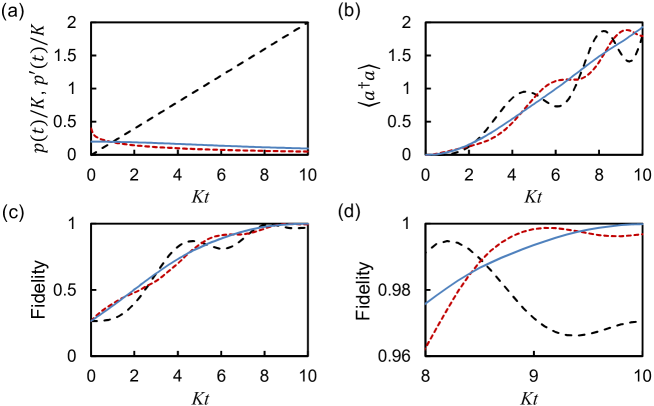
Figure 4: Simulation results for shortcut to adiabaticity. (a) Pump amplitudes, $p(t)$ (black long-dashed line), $p^{\prime}(t)$ in our method (cyan solid line), and $p^{\prime}(t)$ in Ref. 15 (red short-dashed line). (b) Average photon number in KPO, $\langle a^{\dagger}a\rangle$. (c) Fidelity between the final state and the ideal even cat state with amplitude of $\sqrt{2}$. (d) Magnification of (c) around the final time. In (b)–(d), cyan solid, red short-dashed, and black long-dashed lines correspond to our method, the method proposed in Ref. 15, and the case of no $p^{\prime}(t)$ (without shortcut-to-adiabaticity technique), respectively.

References

- (1) S. Haroche, Nobel Lecture: Controlling photons in a box and exploring the quantum to classical boundary, Rev. Mod. Phys. 85, 1083 (2013).
- (2) D. J. Wineland, Nobel Lecture: Superposition, entanglement, and raising Schrödinger’s cat, Rev. Mod. Phys. 85, 1103 (2013).
- (3) U. Leonhardt, Measuring the Quantum State of Light (Cambridge Univ. Press, Cambridge, 1997).
- (4) A. Ourjoumtsev, R. Tualle-Brouri, J. Laurat, and P. Grangier, Generating Optical Schrödinger Kittens for Quantum Information Processing, Science 312, 83 (2006).
- (5) K. Wakui, H. Takahashi, A. Furusawa, and M. Sasaki, Photon subtracted squeezed states generated with periodically poled KTiOPO4, Opt. Ext. 15, 3568 (2007).
- (6) A. Ourjoumtsev, H. Jeong, R. Tualle-Brouri, and P. Grangier, Generation of optical ‘Schrödinger cats’ from photon number states, Nature (London) 448, 784 (2007).
- (7) D. V. Sychev, A. E. Ulanov, A. A. Pushkina, M. W. Richards, I. A. Fedorov, and A. I. Lvovsky, Enlargement of optical Schrödinger’s cat states, Nat. Photon. 11, 379 (2017).
- (8) S. Deléglise, I. Dotsenko, C. Sayrin, J. Bernu, M. Brune, J.-M. Raimond, and S. Haroche, Reconstruction of non-classical cavity field states with snapshots of their decoherence, Nature (London) 455, 510 (2008).
- (9) B. Vlastakis, G. Kirchmair, Z. Leghtas, S. E. Nigg, L. Frunzio, S. M. Girvin, M. Mirrahimi, M. H. Devoret, and R. J. Schoelkopf, Deterministically Encoding Quantum Information Using 100-Photon Schrödinger Cat States, Science 342, 607 (2013).
- (10) Z. Leghtas, S. Touzard, I. M. Pop, A. Kou, B. Vlastakis, A. Petrenko, K. M. Sliwa, A. Narla, S. Shankar, M. J. Hatridge, M. Reagor, L. Frunzio, R. J. Schoelkopf, M. Mirrahimi, and M. H. Devoret, Confining the state of light to a quantum manifold by engineered two-photon loss, Science 347, 853 (2015).
- (11) S. Touzard, A. Grimm, Z. Leghtas, S. O. Mundhada, P. Reinhold, C. Axline, M. Reagor, K. Chou, J. Blumoff, K. M. Sliwa, S. Shankar, L. Frunzio, R. J. Schoelkopf, M. Mirrahimi, and M. H. Devoret, Coherent Oscillations inside a Quantum Manifold Stabilized by Dissipation, Phys. Rev. X 8, 021005 (2018).
- (12) C. Wang, Y. Y. Gao, P. Reinhold, R. W. Heeres, N. Ofek, K. Chou, C. Axline, M. Reagor, J. Blumoff, K. M. Sliwa, L. Frunzio, S. M. Girvin, and L. Jiang, A Schrödinger cat living in two boxes, Science 352, 1087 (2016).
- (13) W. Pfaff, C. J. Axline, L. D. Burkhart, U. Vool, P. Reinhold, L. Frunzio, L. Jiang, M. H. Devoret, and R. J. Schoelkopf, Controlled release of multiphoton quantum states from a microwave cavity memory, Nat. Phys. 13, 882 (2017).
- (14) H. Goto, Bifurcation-based adiabatic quantum computation with a nonlinear oscillator network, Sci. Rep. 6, 21686 (2016).
- (15) S. Puri, S. Boutin, and A. Blais, Engineering the quantum states of light in a Kerr-nonlinear resonator by two-photon driving, npj Quant. Inf. 3, 18 (2017).
- (16) H. Goto, Universal quantum computation with a nonlinear oscillator network, Phys. Rev. A 93, 050301(R) (2016).
- (17) S. E. Nigg, N. Lörch, and R. P. Tiwari, Robust quantum optimizer with full connectivity, Sci. Adv. 3, e1602273 (2017).
- (18) S. Puri, C. K. Andersen, A. L. Grimsmo, and A. Blais, Quantum annealing with all-to-all connected nonlinear oscillators, Nat. Commun. 8, 15785 (2017).
- (19) Z. R. Lin, et al. Josephson parametric phase-locked oscillator and its application to dispersive readout of superconducting qubits, Nat. Commun. 5, 4480 (2014).
- (20) C. W. Gardiner and M. J. Collett, Input and output in damped quantum systems: Quantum stochastic differential equations and the master equation, Phys. Rev. A 31, 3761 (1985).
- (21) D. F. Walls and G. J. Milburn, Quantum Optics (Springer, Berlin, 1994).
- (22) L.-M. Duan, A. Kuzmich, and H. J. Kimble, Cavity QED and quantum-information processing with “hot” trapped atoms, Phys. Rev. A 67, 032305 (2003).
- (23) H. Goto and K. Ichimura, Quantum trajectory simulation of controlled phase-flip gates using the vacuum Rabi splitting, Phys. Rev. A 72, 054301 (2005).
- (24) In this work, we assume a negative Kerr coefficient as in the case of Josephson parametric oscillators Lin2014a . If the Kerr coefficient is positive, we flip the sign of the pump amplitude to obtain the same results.
- (25) C. Eichler, D. Bozyigit, C. Lang, L. Steffen, J. Fink, and A. Wallraff, Experimental State Tomography of Itinerant Single Microwave Photons, Phys. Rev. Lett. 106, 220503 (2011).
- (26) See Appendix for the detailed methods and results of the present numerical simulations, the pulse shape control of the pump amplitude using low-pass filters, and the derivation of the counterdiabatic Hamiltonian for our shortcut-to-adiabaticity technique.
- (27) H. M. Wiseman and G. J. Milburn, Quantum Measurement and Control (Cambridge University Press, Cambridge, 2010).
- (28) C. Eichler, D. Bozyigit, and A. Wallraff, Characterizing quantum microwave radiation and its entanglement with superconducting qubits using linear detectors, Phys. Rev. A 86, 032106 (2012).
- (29) M. Demirplak and S. A. Rice, Adiabatic Population Transfer with Control Fields, J. Phys. Chem. A 107, 9937 (2003).
- (30) A. del Campo, Shortcuts to Adiabaticity by Counterdiabatic Driving, Phys. Rev. Lett. 111, 100502 (2013).
- (31) A shortcut-to-adiabaticity technique for a KPO has been proposed in Ref. 15. This also uses an imaginary pump amplitude , but the definition of is different from the present one in Eq. (12). We found that our definition of outperforms the definition proposed in Ref. 15. See Appendix C for the details.